Enda Moloney

05367981

B.E. Electronic Engineering Project Report

EE426

Classification of Electrocardiogram (ECG) Waveforms

for the Detection of Cardiac Problems

March 2009

2

Abstract

The primary aim of this project is to design a computer-based system for the

processing and classification of Electrocardiogram waveforms with the intention of

assisting in the detection of abnormalities and therefore facilitate the early detection

of cardiac problems. Important features of the ECG waveform such as the timing of

significant events are obtained. Individual waveforms are examined. The Pan-

Tompkins algorithm and the Fourier Transform for the ECG signals are discussed.

There is a review of Artificial Neural Network (ANN) and how it can be applied to

ECG data. The report concludes with a summary of results and suggestions for future

work.

3

Acknowledgements

I would like to thank Dr. Edward Jones for all his help, guidance and assistance in this

project throughout the year. I would like to also thank my family for all their help and

encouragement during the last four years.

4

Declaration of Originality

I declare that my thesis is original work except where otherwise stated.

Signature: Data:

5

Table of contents

Abstract ..................................................................................................................... 2

Acknowledgements ................................................................................................... 3

Declaration of Originality .......................................................................................... 4

Table of contents ....................................................................................................... 5

1.0 Introduction ......................................................................................................... 6

2.0 Physiological Background ................................................................................... 8

2.1 The Heart and ECG waveform ............................................................................. 8

2.2 History of ECG.................................................................................................. 10

2.3 ECG signals ....................................................................................................... 12

3.0 System Overview .............................................................................................. 15

3.1 From signals to samples ..................................................................................... 15

3.2 MIT-BIT Database ............................................................................................ 16

4.0 QRS Detection................................................................................................... 19

4.1 Introduction ....................................................................................................... 19

4.2 Pan-Tompkins algorithm ................................................................................... 20

4.3 Finding the QRS peaks ...................................................................................... 23

4.4 Getting individual beats ..................................................................................... 24

4.5 Exact times of the QRS complex ....................................................................... 25

5.0 Fourier Analysis ................................................................................................ 26

5.1 Fourier Transform ............................................................................................. 26

5.2 Fast Fourier Transform ...................................................................................... 27

5.3 Implementation of the Fourier Transform .......................................................... 29

6.0 Artificial Neural Network .................................................................................. 32

6.1 ANN as applied to ECG signals ......................................................................... 32

7.0 Results and Conclusion ...................................................................................... 35

8.0 References ......................................................................................................... 42

8.1 Bibliography ...................................................................................................... 43

9.0 Appendix ........................................................................................................... 44

6

1.0 Introduction

The primary aim of this project is to design a computer-based system for the

processing and classification of Electrocardiogram waveforms with the intention of

assisting in the detection of abnormalities and hence facilitating early detection of

cardiac problems. Cardiac arrhythmias are malfunctions of the heart, which if left

untreated could result in serious health problems. The project uses software called

MATLAB programming language; this detects and diagnoses problems.

Such a system would not be intended to replace a human cardiac specialist;

rather it would be intended to “flag” patients with potential heart problems, thus

enabling early referral to a specialist.

A goal of the project is to compare a number of approaches to the problem, based on

criteria such as performance as well as computational complexity. For development

purposes, the MIT-BIH database of ECG waveforms and corresponding annotations

can be used for test data. All problems associated with each wave have already been

identified in the MIT-BIH database.

The Fast Fourier Transform is applied to these ECG waves to extract

information about them and using Artificial Neural Network they are divided into

different classes. Information about the duration of the QRS complex was extracted

from the ECG wave; this can be used to detect abnormalities.

This report is presented in a number of chapters as follows: Chapter 2 gives an

explanation of the working of the heart and the various features of the ECG signals.

Chapter 3 reviews the algorithm used in the project. Chapter 4 discusses QRS

detection and the Pan-Tompkins algorithm. Chapter 5 reviews the Fourier Transform

7

and how it can be applied to the ECG signal. Chapter 6 reviews the uses of Artificial

Neural Network as applied to ECG signals. The concluding chapter presents results

and conclusions with suggestions for future work. At the end of the report there are

references, bibliography and an appendix.

8

2.0 Physiological Background

This chapter reviews the working of the heart and how it produces ECG

waves. The history of measurement of an ECG signal is explained. The characteristic

features of an ECG signal are outlined.

2.1 The Heart and ECG waveform

The heartbeat is started by a „pacemaker‟ called the sinoatrial node (SA node)

as shown in Fig 2.1. It is situated in the right atrium near the point where the venae

cavae enter. This node is a specialised area of heart muscle that generates electrical

impulses. The electrical impulse travels to the atrioventicular (AV) node. Here there is

a very brief delay to allow atria to contract. From the AV node the electrical impulse

spreads into Purkinje fibres causing ventricles to contract. This complete cardiac cycle

takes place about 70 times in one minute. Each cycle takes about 0.8 of a second. An

electrocardiogram (ECG) is a recording of the electrical activity of the heart as

electrical signal spreads from the right atrium to the left atrium.

9

Figure 2.1: Heart

.The ECG is a recording of the electrical activity at a fixed rate and a graph is plotted

of voltage on y-axis against time on the x-axis.

There are a wide variety of uses for ECG such as:

Determining if the heart is performing normally or suffering from

abnormalities such as extra or skipped heartbeats.

Indicating previous damage to the heart muscle.

Providing information on the physical condition of the heart.

Been used to detect non-cardiac diseases (e.g. Pulmonary embolism,

hypothermia).

10

2.2 History of ECG

In the

nineteenth century it was difficult to measure the electrical signal for the

heart; moving coil galvanometers were not sensitive enough to measure the tiny

electric currents. A breakthrough came in 1901 when Einthoven invented the string

galvanometer. [1] This device was more sensitive than the capillary electrometer that

Waller used and the string galvanometer that had been invented separately in 1897 by

the French engineer, Ader.

The electrical activity of heart can be measured by an array of electrodes

placed on the body. The recorded tracing is called ECG. The different waves

represent the sequence of contraction and relaxation of the atria and ventrials. [2]

ECG is recorded at a speed of 25mm/sec and voltage is calibrated so that 1mV =

10mm in the vertical direction. Therefore each small 1mm square in figure 1

represents 0.04 sec in time and 0.1mV in voltage, as shown in fig. 2.2

Figure 2.2: A "typical" ECG tracing

Einthoven assigned the letters P, Q, R, S and T to the various deflections, and

described the electrocardiographic features of a number of cardiovascular disorders.

11

The meaning of these letters is discussed in more details later. In 1924 he was

awarded the Nobel Prize in Medicine for his discovery.

Though the basic principles of that era are still in use today, there have been many

advances in electrocardiography over the years. The instrumentation, for example, has

evolved from a cumbersome laboratory apparatus to compact electronic systems that

often include computerized interpretation of the electrocardiogram.

Einthoven‟s string galvanometer is known as Einthoven‟s triangle because

three leads were used which were literally placed on the arms and legs in buckets of

salt water in order to obtain a electrical signal. Electrodes were later invented which

could be place directly on the patient‟s skin and they are still placed on the arms and

legs.

They are the first three leads of the now twelve leads that are used in the

modern ECG., as shows in fig. 2.3.

Fig 2.3: Placement of the leads on limbs

12

A lead 1 is a dipole negative electrode (white) on the RA and positive (black)

electrode on LA.

Lead 2 is a dipole with negative electrode (white) on RA and positive (red) electrode

on LL.

Lead 3 is dipole with negative (black) electrode on LA and positive (red) on LL

2.3 ECG signals

An ECG is constructed by measuring the electrical potential between various

points of the body using leads. The normal ECG wave is composed of

1. The P wave

2. QRS complex

3. ST segment

4. The T wave

5. U wave

The relationship between P waves and QRS complexes helps distinguish various

cardiac irregularities. Below is a computer generated image of a healthy ECG trace.

Fig 2.4: Representation of ECG wave

13

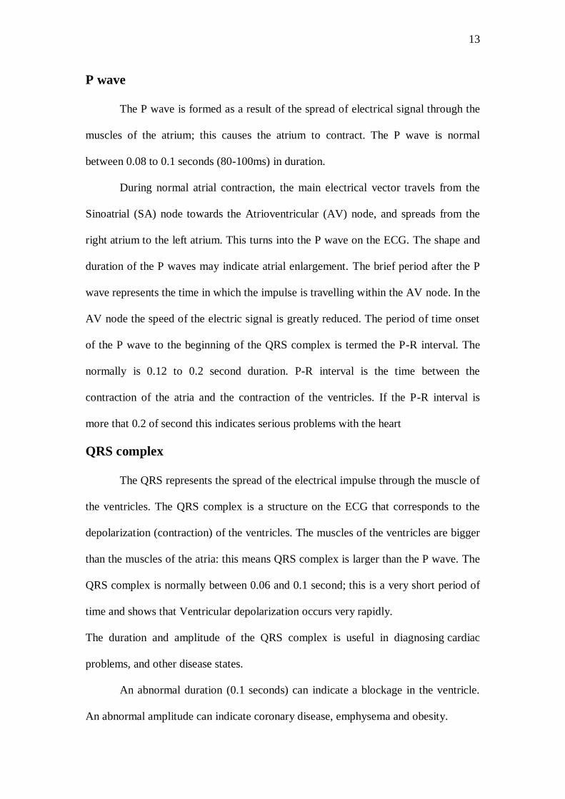
P wave

The P wave is formed as a result of the spread of electrical signal through the

muscles of the atrium; this causes the atrium to contract. The P wave is normal

between 0.08 to 0.1 seconds (80-100ms) in duration.

During normal atrial contraction, the main electrical vector travels from the

Sinoatrial (SA) node towards the Atrioventricular (AV) node, and spreads from the

right atrium to the left atrium. This turns into the P wave on the ECG. The shape and

duration of the P waves may indicate atrial enlargement. The brief period after the P

wave represents the time in which the impulse is travelling within the AV node. In the

AV node the speed of the electric signal is greatly reduced. The period of time onset

of the P wave to the beginning of the QRS complex is termed the P-R interval. The

normally is 0.12 to 0.2 second duration. P-R interval is the time between the

contraction of the atria and the contraction of the ventricles. If the P-R interval is

more that 0.2 of second this indicates serious problems with the heart

QRS complex

The QRS represents the spread of the electrical impulse through the muscle of

the ventricles. The QRS complex is a structure on the ECG that corresponds to the

depolarization (contraction) of the ventricles. The muscles of the ventricles are bigger

than the muscles of the atria: this means QRS complex is larger than the P wave. The

QRS complex is normally between 0.06 and 0.1 second; this is a very short period of

time and shows that Ventricular depolarization occurs very rapidly.

The duration and amplitude of the QRS complex is useful in diagnosing cardiac

problems, and other disease states.

An abnormal duration (0.1 seconds) can indicate a blockage in the ventricle.

An abnormal amplitude can indicate coronary disease, emphysema and obesity.

14

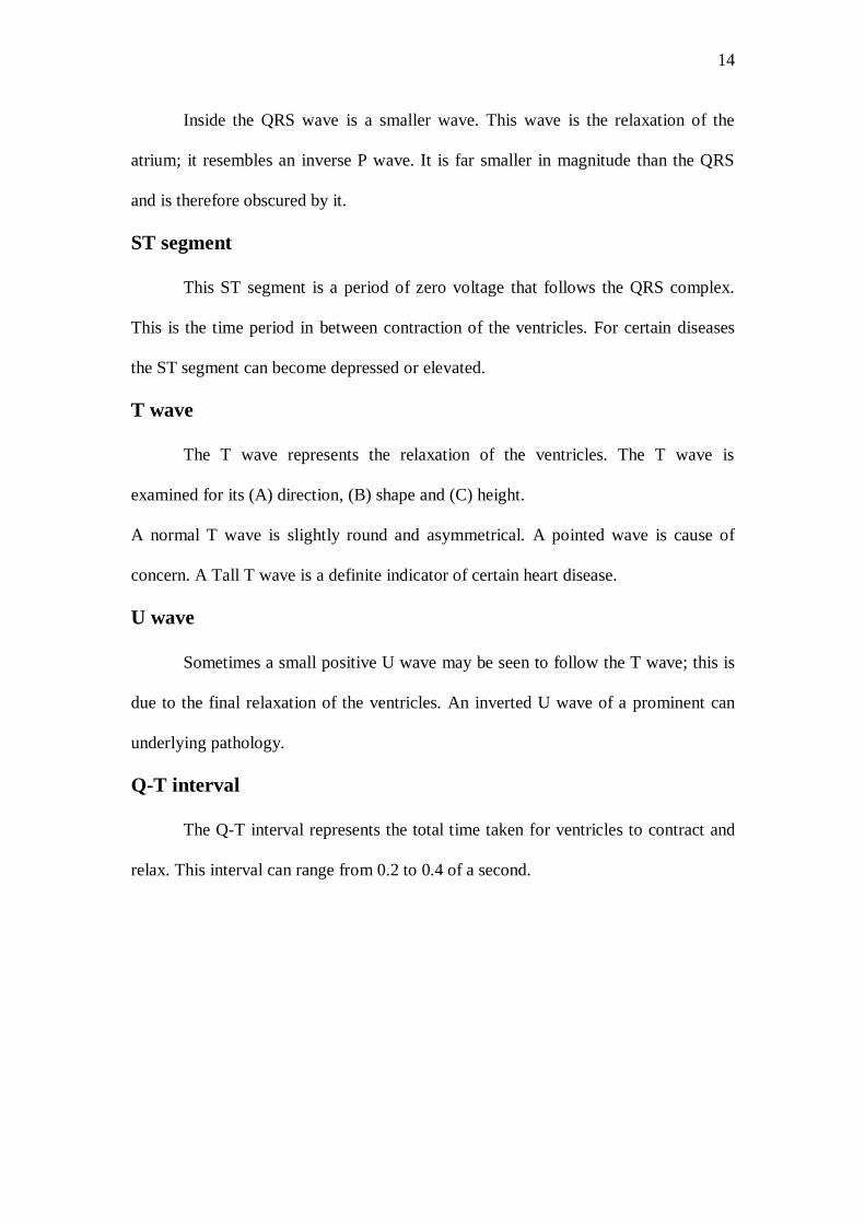
Inside the QRS wave is a smaller wave. This wave is the relaxation of the

atrium; it resembles an inverse P wave. It is far smaller in magnitude than the QRS

and is therefore obscured by it.

ST segment

This ST segment is a period of zero voltage that follows the QRS complex.

This is the time period in between contraction of the ventricles. For certain diseases

the ST segment can become depressed or elevated.

T wave

The T wave represents the relaxation of the ventricles. The T wave is

examined for its (A) direction, (B) shape and (C) height.

A normal T wave is slightly round and asymmetrical. A pointed wave is cause of

concern. A Tall T wave is a definite indicator of certain heart disease.

U wave

Sometimes a small positive U wave may be seen to follow the T wave; this is

due to the final relaxation of the ventricles. An inverted U wave of a prominent can

underlying pathology.

Q-T interval

The Q-T interval represents the total time taken for ventricles to contract and

relax. This interval can range from 0.2 to 0.4 of a second.

15

3.0 System Overview

This chapter gives a system overview of the project. Example can get sample

of ECG signals and what process can be applied to them.

3.1 From signals to samples

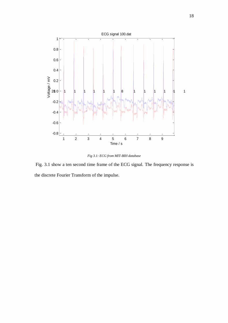
In the previous chapter we saw that the heart produces an ECG signal which

can be monitored. For research purpose, ECG signals have been collected and stored

in a database, called the MIT-BIH database. The signal are examined with the Pan-

Tompkins algorithm and then sent for Fourier analysis. Finally the results are sent to

16

the Artificial Neural Network. This can be representing by a flow-chart as follow:

Individual

Beats

Find Times of P, Q, R, Fast Fourier Transform

ECG Signal

MIT-BIT Database

Pan Tomkins Ailgorithm

Time for QRS ComplexFrequency Response

Of Beats

3.2 MIT-BIT Database

In the 1970s Beth Israel Hospital (BIH) and Massachusetts Institute of

Technology (MIT) collaborated in research into arrhythmia. [3] They examined the

hospital records to produce a database of ECG waveforms. From hospital records

twenty three recording were picked at random from a set of 4000. Twenty five records

with abnormal ECG were also collect for the same data. This is done on purpose for

17

research, as out of forty eight records you would not usually get twenty five abnormal

records. Each record was independently noted with an explanation, to include

background information on the subjects, including their medications. Each record is

thirty minutes long and was digitized at 360 samples per second: this gives 648,000

samples in a 30 minute record. To analyse these records a MATLAB program was

used [4].

MATLAB stand for matrix laboratory. It is a computer programming language

developed in the 1970 by Cleve Moler to replace Fortran. Today it is used by

engineers all over the world.

In each record there are three files that make up the data; the hea file, atr file

and a dat file. To interpret this file we use a MATLAB program created by Robert

Tratnig (Vorarlberg University) was used. The MIT-BIH database was encoded in the

212 format. Robert Tratnig‟s code converted the database to binary data. This data

was used throughout the project. In the programme, the number of samples to be read

can be adjusted up to a maximum 648,000 samples. This point proved to be important

when graphing the data.

18

1 2 3 4 5 6 7 8 9

-0.8

-0.6

-0.4

-0.2

0

0.2

0.4

0.6

0.8

1

281 1 1 1 1 1 1 8 1 1 1 1 1 1 1 1 1 1 1 1 1 1 1 1 1 1 1 1 1 1 1 1 1 1 1 1 1 1 1 1 1 1 1 1 1 1 1 1 1 1 1 1 1 1 1 1 1 1 1 1 1 1 1 1 1 1 1 1 1 1 1 1 1 1 1 1 1 1 1 1 1 1 1 1 1 1 1 1 1 1 1 1 1 1 1 1 1 1 1 1 1 1 1

Time / s

Voltage /

mV

ECG signal 100.dat

Fig 3.1: ECG from MIT-BIH database

Fig. 3.1 show a ten second time frame of the ECG signal. The frequency response is

the discrete Fourier Transform of the impulse.

19

4.0 QRS Detection

Chapter 4 explains the importance of the QRS complex and the Pan-Tompkins

algorithm to detect it. Using the Algorithm, the R peak in the QRS complex can be

found; this leads to getting the exact duration of the QRS complex.

4.1 Introduction

The QRS complex is the most important complex in the ECG. The duration

and amplitude should be measured as accurately as possible. There are two methods

for highlight the QRS complex [5]:

1. Derivative-based methods.

2. Pan-Tompkins algorithm.

Derivative-based methods depend on the fact that the QRS complex has the

greatest slope and the sharpest turning point. It is also the highest point in the cardiac

cycle. Rate of change is another name for the sharpest turning point, and we can find

this using the derivative operator (d/dt). In principle the derivative operator will

suppresses the P and T waves and highlight the QRS complex. However inside the

QRS wave is a smaller wave; this is due to the relaxation of the atrium. While the

wave can not be seen it gives rise to a peak above the QRS complex for a very short

time interval. A QRS detection method based only on the derivative operator will

give misleading results.

In 1985 Pan and Tompkins proposed a new method for detection: the QRS

complex. This method is an advance on the derivative-based method and also tries to

eliminate noise for the ECG signal. This is now called the Pan-Tompkins algorithm.

20

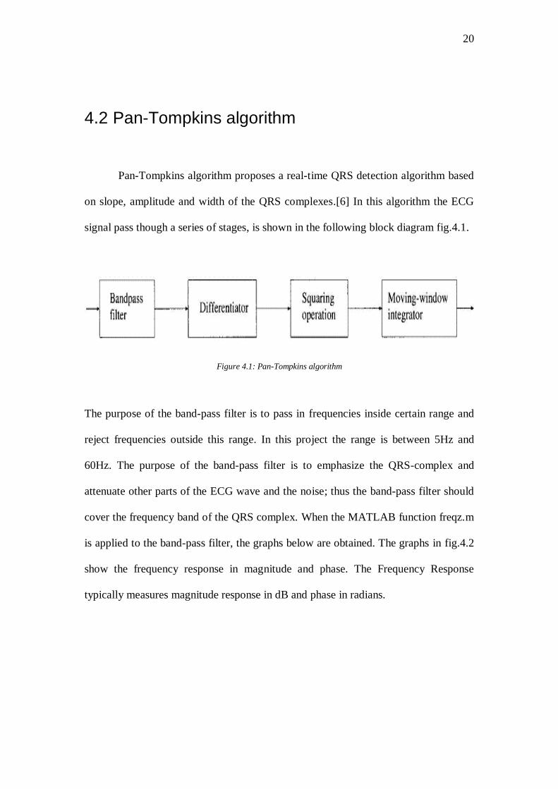
4.2 Pan-Tompkins algorithm

Pan-Tompkins algorithm proposes a real-time QRS detection algorithm based

on slope, amplitude and width of the QRS complexes.[6] In this algorithm the ECG

signal pass though a series of stages, is shown in the following block diagram fig.4.1.

Figure 4.1: Pan-Tompkins algorithm

The purpose of the band-pass filter is to pass in frequencies inside certain range and

reject frequencies outside this range. In this project the range is between 5Hz and

60Hz. The purpose of the band-pass filter is to emphasize the QRS-complex and

attenuate other parts of the ECG wave and the noise; thus the band-pass filter should

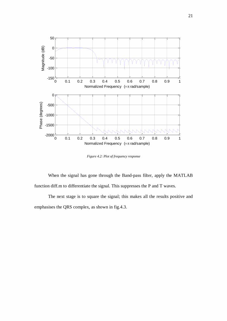
cover the frequency band of the QRS complex. When the MATLAB function freqz.m

is applied to the band-pass filter, the graphs below are obtained. The graphs in fig.4.2

show the frequency response in magnitude and phase. The Frequency Response

typically measures magnitude response in dB and phase in radians.

21

0 0.1 0.2 0.3 0.4 0.5 0.6 0.7 0.8 0.9 1-2000

-1500

-1000

-500

0

Normalized Frequency ( rad/sample)

Phase (

degre

es)

0 0.1 0.2 0.3 0.4 0.5 0.6 0.7 0.8 0.9 1-150

-100

-50

0

50

Normalized Frequency ( rad/sample)

Magnitude (

dB

)

Figure 4.2: Plot of frequency response

When the signal has gone through the Band-pass filter, apply the MATLAB

function diff.m to differentiate the signal. This suppresses the P and T waves.

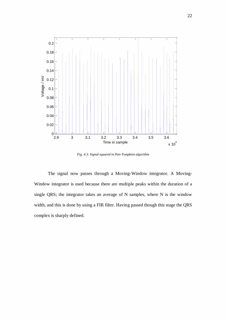
The next stage is to square the signal; this makes all the results positive and

emphasises the QRS complex, as shown in fig.4.3.

22

2.9 3 3.1 3.2 3.3 3.4 3.5 3.6

x 104

0

0.02

0.04

0.06

0.08

0.1

0.12

0.14

0.16

0.18

0.2

Time in sample

Voltage /

mV

Fig. 4.3: Signal squared in Pan-Tompkins algorithm

The signal now passes through a Moving-Window integrator. A Moving-

Window integrator is used because there are multiple peaks within the duration of a

single QRS; the integrator takes an average of N samples, where N is the window

width, and this is done by using a FIR filter. Having passed though this stage the QRS

complex is sharply defined.

23

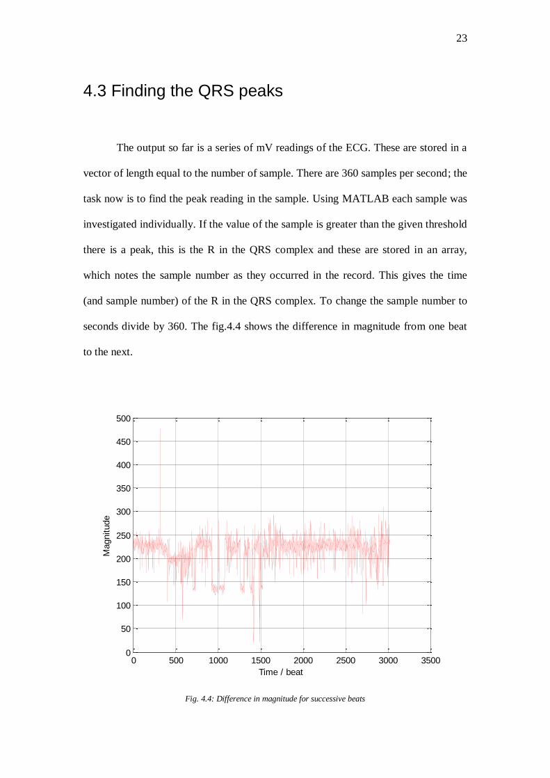
4.3 Finding the QRS peaks

The output so far is a series of mV readings of the ECG. These are stored in a

vector of length equal to the number of sample. There are 360 samples per second; the

task now is to find the peak reading in the sample. Using MATLAB each sample was

investigated individually. If the value of the sample is greater than the given threshold

there is a peak, this is the R in the QRS complex and these are stored in an array,

which notes the sample number as they occurred in the record. This gives the time

(and sample number) of the R in the QRS complex. To change the sample number to

seconds divide by 360. The fig.4.4 shows the difference in magnitude from one beat

to the next.

0 500 1000 1500 2000 2500 3000 35000

50

100

150

200

250

300

350

400

450

500

Time / beat

Magnitude

Fig. 4.4: Difference in magnitude for successive beats

24

4.4 Getting individual beats

Using MATLAB a programme was devised which went through all the

samples again. Using subtraction, the programme found the sample number half way

between each beat. For example: Suppose there are beats at:

Sample[60,70,84].

S1 = Sample (j) + 0.5(Sample (j+1) – Sample (j))

S1 = 60 + 0.5(70-60) = 65

S2 = Sample (j+1) + 0.5(Sample (j+2) – Sample (j+1))

S2 = 70 + 0.5(84-70) = 77

The output from this part of the programme is shown in fig.4.5:

0 50 100 150 200 250-1

-0.5

0

0.5

1

1.5

Sample numbers

Voltage /

mV

Fig. 4.5: One complete cardiac cycles

The points P, Q, R, S and T are clearly visible on this graph.

25

4.5 Exact times of the QRS complex

From the data obtained so far, it is possible to find the exact time of the R

complex. This is important for pattern recognition of a heart beat. The time of the R

complex was found by using the max function of MATLAB on one complete cardiac

cycle.

In the example mentioned previously there is a peak at sample 70; so a

complete cycle goes from samples 65 to 77.

If there is a peak at sample 70, the min function in MATLAB will find the

lowest point between samples 65 and 70, i.e. the Q complex.

If the function is applied to samples 70 to 77, then the S complex will be

found.

A similar process could be applied to find the max at P and T; this could be

more difficult as the P and T peaks are not as pronounced. Finally, if the time for Q

and S are known the times of the QRS complex can be found.

The duration of the QRS complex is usually 0.06 seconds (60ms) to 0.1

seconds (10ms). If the duration of the QRS complex is prolonged more than 0.1 sec, it

is an indicator of certain heart diseases.

26

5.0 Fourier Analysis

Chapter 5 outline the 19th

century Fourier Transform and the 20th

century Fast

Fourier Transform. The Fast Fourier Transform is implemented by using a direct

command in MATLAB.

5.1 Fourier Transform

Fourier analysis is a family of mathematical techniques; all based on

decomposing signals into sin and cosine functions. Fourier analysis and its transform

are called after Joseph Fourier, a French mathematician and physicist in the 1800s. [7]

In 1822 he published his famous work, Theorie analytique de La chaleur (the

analytical theory of heat). This was the first work to use the Fourier series. He is also

credited with the discovery of the greenhouse effect in 1824. Fourier laid the

foundation for the Fast Fourier Transform which is used by scientists and engineers

today.

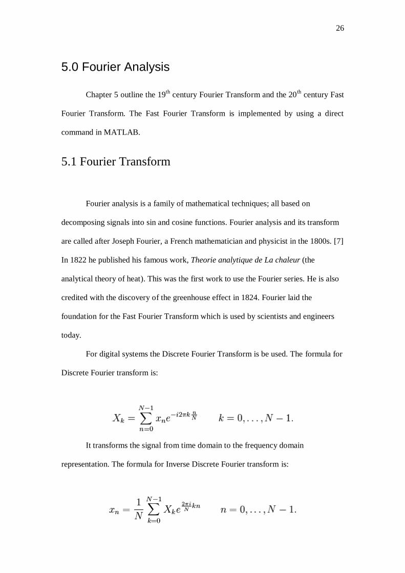
For digital systems the Discrete Fourier Transform is be used. The formula for

Discrete Fourier transform is:

It transforms the signal from time domain to the frequency domain

representation. The formula for Inverse Discrete Fourier transform is:

27

It transforms the signal from frequency domain back to the time domain

representation. Both these formulas require very lengthy calculation.

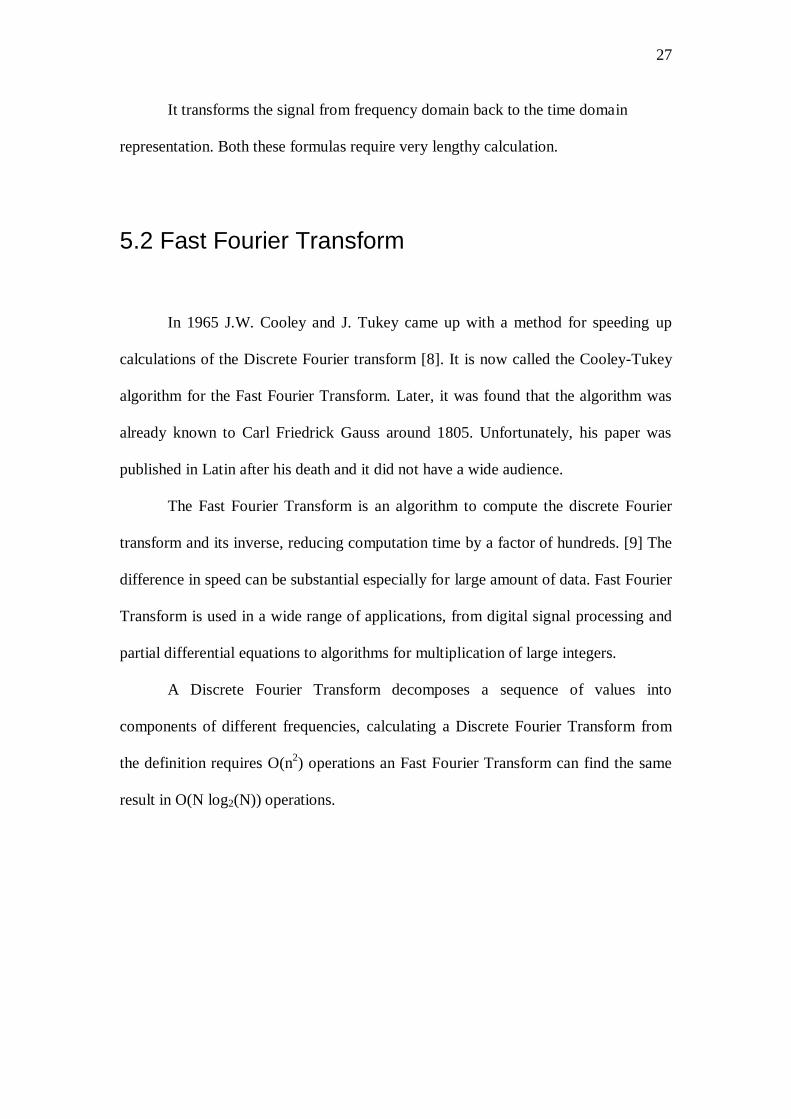
5.2 Fast Fourier Transform

In 1965 J.W. Cooley and J. Tukey came up with a method for speeding up

calculations of the Discrete Fourier transform [8]. It is now called the Cooley-Tukey

algorithm for the Fast Fourier Transform. Later, it was found that the algorithm was

already known to Carl Friedrick Gauss around 1805. Unfortunately, his paper was

published in Latin after his death and it did not have a wide audience.

The Fast Fourier Transform is an algorithm to compute the discrete Fourier

transform and its inverse, reducing computation time by a factor of hundreds. [9] The

difference in speed can be substantial especially for large amount of data. Fast Fourier

Transform is used in a wide range of applications, from digital signal processing and

partial differential equations to algorithms for multiplication of large integers.

A Discrete Fourier Transform decomposes a sequence of values into

components of different frequencies, calculating a Discrete Fourier Transform from

the definition requires O(n2) operations an Fast Fourier Transform can find the same

result in O(N log2(N)) operations.

28

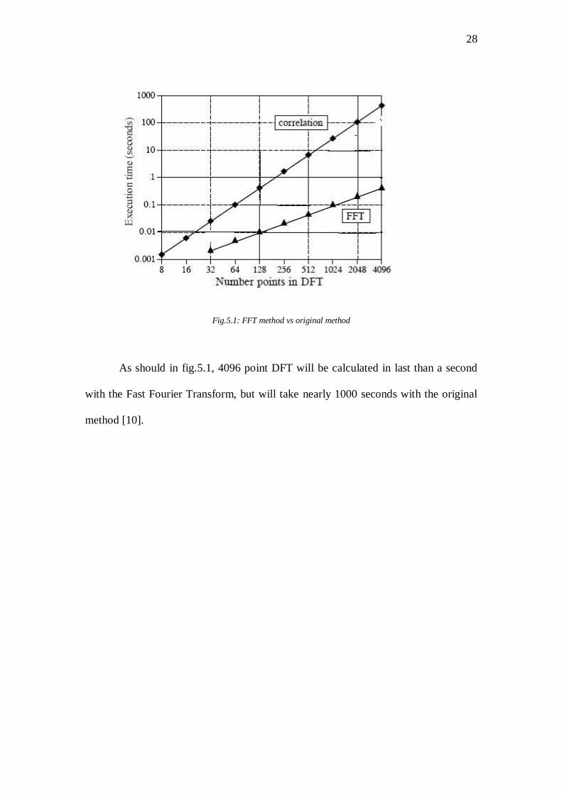
Fig.5.1: FFT method vs original method

As should in fig.5.1, 4096 point DFT will be calculated in last than a second

with the Fast Fourier Transform, but will take nearly 1000 seconds with the original

method [10].

29

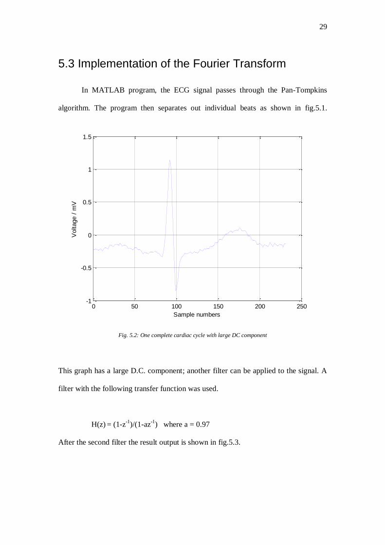
5.3 Implementation of the Fourier Transform

In MATLAB program, the ECG signal passes through the Pan-Tompkins

algorithm. The program then separates out individual beats as shown in fig.5.1.

0 50 100 150 200 250-1

-0.5

0

0.5

1

1.5

Sample numbers

Voltage /

mV

Fig. 5.2: One complete cardiac cycle with large DC component

This graph has a large D.C. component; another filter can be applied to the signal. A

filter with the following transfer function was used.

H(z) = (1-z-1

)/(1-az-1

) where a = 0.97

After the second filter the result output is shown in fig.5.3.

30

0 50 100 150 200 250-1

-0.5

0

0.5

1

1.5

Sample numbers

Voltage /

mV

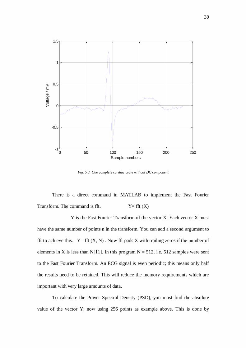
Fig. 5.3: One complete cardiac cycle without DC component

There is a direct command in MATLAB to implement the Fast Fourier

Transform. The command is fft. Y= fft (X)

Y is the Fast Fourier Transform of the vector X. Each vector X must

have the same number of points n in the transform. You can add a second argument to

fft to achieve this. Y= fft (X, N) . Now fft pads X with trailing zeros if the number of

elements in X is less than N[11]. In this program N = 512, i.e. 512 samples were sent

to the Fast Fourier Transform. An ECG signal is even periodic; this means only half

the results need to be retained. This will reduce the memory requirements which are

important with very large amounts of data.

To calculate the Power Spectral Density (PSD), you must find the absolute

value of the vector Y, now using 256 points as example above. This is done by

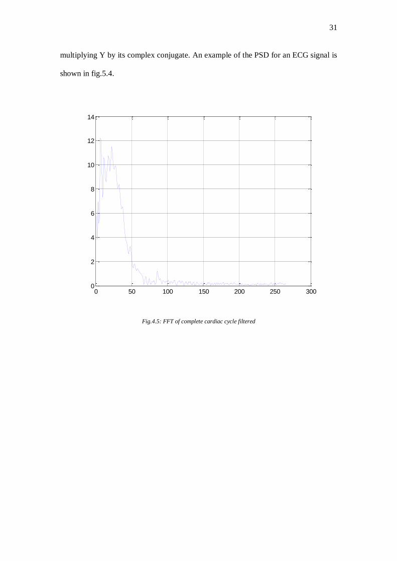
31

multiplying Y by its complex conjugate. An example of the PSD for an ECG signal is

shown in fig.5.4.

0 50 100 150 200 250 3000

2

4

6

8

10

12

14

Fig.4.5: FFT of complete cardiac cycle filtered

32

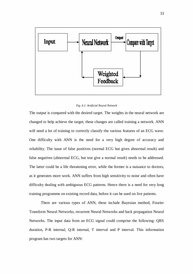
6.0 Artificial Neural Network

This Chapter explain how a Artificial Neural Network operates the long

training programme for ECG data is outlined. The importance of getting reliable

results is emphasised.

6.1 ANN as applied to ECG signals

When the ECG waves have been processed, they must be classified into 2

classes: normal or abnormal. As the ECG wave is very complex 2 classes will not be

sufficient. In this project the classifier that will be used is the Artificial Neural

Network (ANN).

AAN is a computer based system based on the Neural Networks in human

biology. Neural Networks are useful for pattern recognition and non-linear systems.

The function of network depends on the connection between the different elements

(neurons). These connections are called weights. The basic processes are shown in

fig.6.1.

33

Fig. 6.1: Artificial Neural Network

The output is compared with the desired target. The weights in the neural network are

changed to help achieve the target; these changes are called training a network. ANN

will need a lot of training to correctly classify the various features of an ECG wave.

One difficulty with ANN is the need for a very high degree of accuracy and

reliability. The issue of false positives (normal ECG but gives abnormal result) and

false negatives (abnormal ECG, but test give a normal result) needs to be addressed.

The latter could be a life threatening error, while the former is a nuisance to doctors,

as it generates more work. ANN suffers from high sensitivity to noise and often have

difficulty dealing with ambiguous ECG patterns. Hence there is a need for very long

training programme on existing record data, before it can be used on live patients.

There are various types of ANN, these include Bayesian method, Fourier

Transform Neural Networks, recurrent Neural Networks and back propagation Neural

Networks. The input data from an ECG signal could comprise the following: QRS

duration, P-R internal, Q-R internal, T interval and P interval. This information

program has two targets for ANN:

34

1. Direct classification normal / abnormal

2. Probability result from Direct classification associated with it.

The input data from the ECG should be divided into 2 sections: training data

and testing data. Each result from the testing data will have a probability associated

with it. A probability of 0.8 or 0.9 is fairly certain, but what about 0.5? This result has

only a 50% probability of being right, i.e. it is very uncertain. It might be better to

have 3 classifications (Normal, Abnormal and Uncertain). At least in the initial stages

of training and testing. This system would reduce workload of doctors, and would

now have to review only the uncertain cases. [12]

As people live longer, there are an increasing number of people with heart

trouble who need constant monitoring. An automated computer system using ANN

would reduce the work load of doctor in busy hospitals.

35

7.0 Results and Conclusion

This chapter presents the results which were obtained during the project.

Suggestions for further work are also given.

The following results were obtained during the project. A sample ECG signal

was obtained from the MIT-BIH database. A 1.8 second time frame from the database

is shown in fig.7.1.

0 0.2 0.4 0.6 0.8 1 1.2 1.4 1.6 1.8-0.6

-0.4

-0.2

0

0.2

0.4

0.6

0.8

1

28 1 1

Time / s

Voltage /

mV

ECG signal 100.dat

Figure 7.1: 1.8 second time frame of ECG from MIT-BIT database

The ECG signal passes through a band-pass filter and the frequency response in

shown fig. 7.2.

36

0 0.1 0.2 0.3 0.4 0.5 0.6 0.7 0.8 0.9 1-2000

-1500

-1000

-500

0

Normalized Frequency ( rad/sample)

Phase (

degre

es)

0 0.1 0.2 0.3 0.4 0.5 0.6 0.7 0.8 0.9 1-150

-100

-50

0

50

Normalized Frequency ( rad/sample)

Magnitude (

dB

)

Fig. 7.2 Plot of frequency Response

37

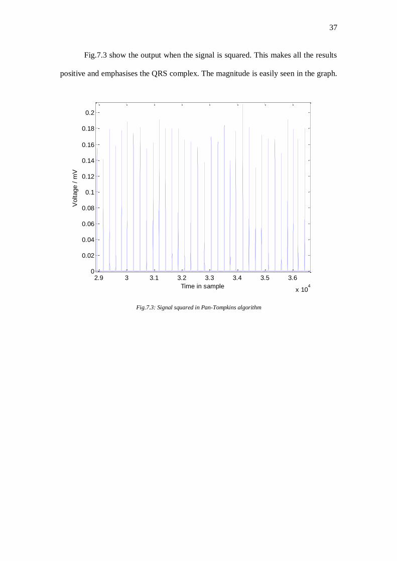
Fig.7.3 show the output when the signal is squared. This makes all the results

positive and emphasises the QRS complex. The magnitude is easily seen in the graph.

2.9 3 3.1 3.2 3.3 3.4 3.5 3.6

x 104

0

0.02

0.04

0.06

0.08

0.1

0.12

0.14

0.16

0.18

0.2

Time in sample

Voltage /

mV

Fig.7.3: Signal squared in Pan-Tompkins algorithm

38

0 50 100 150 200 250-1

-0.5

0

0.5

1

1.5

Sample numbers

Voltage /

mV

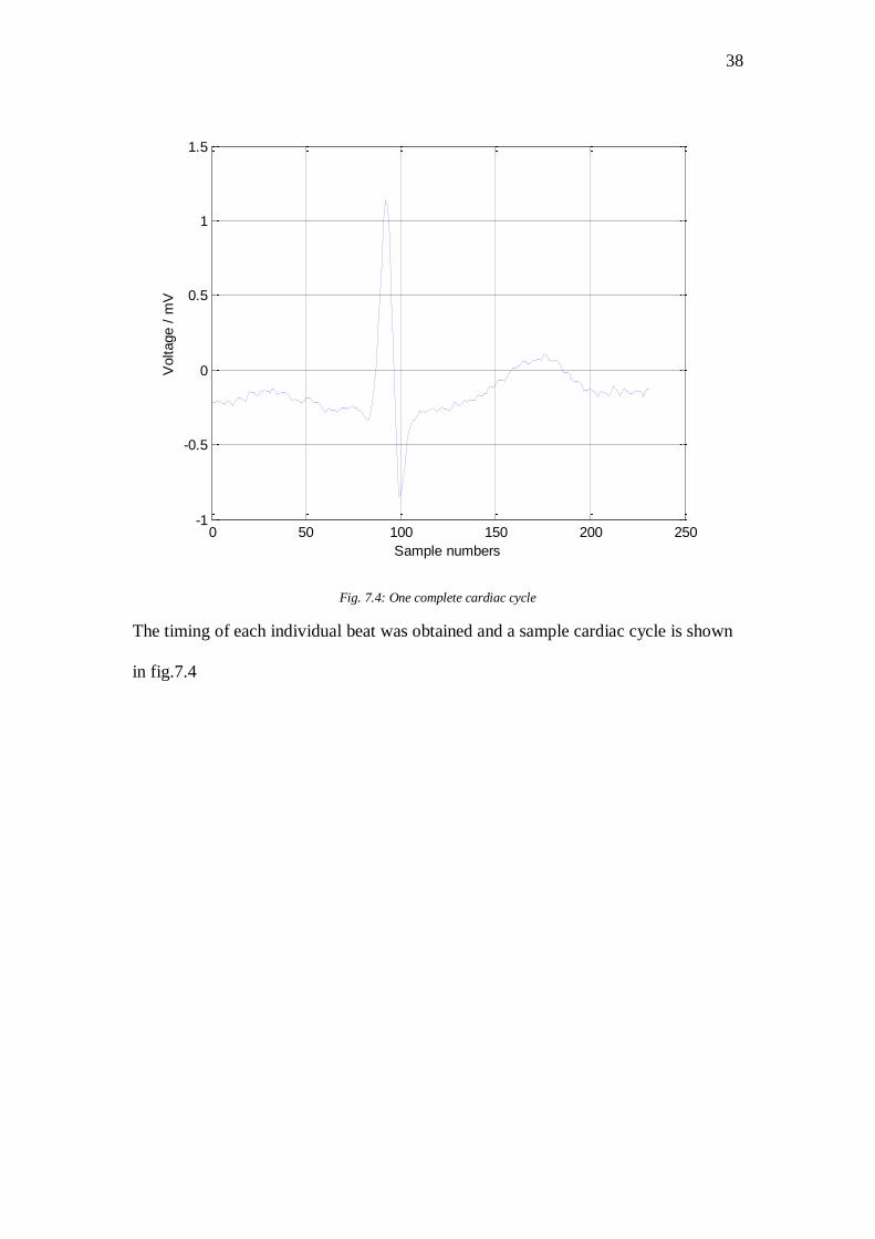
Fig. 7.4: One complete cardiac cycle

The timing of each individual beat was obtained and a sample cardiac cycle is shown

in fig.7.4

39

0 100 200 300 400 500 6000

2

4

6

8

10

12

14

Fig. 7.5: FFT of cardiac cycle

Fig.7.5 show the output from the Fast Fourier Transform for the data using 512

points. An ECG signal is even periodic; this means that only half the results need to

be retained.

40

0 50 100 150 200 250 3000

2

4

6

8

10

12

14

Figure 7.6: Half the FFT of cardiac cycle

Fig. 7.6 show half FFT which is all that needs to be taken into account for

analysis.

Areas of the project that could be developed further are:

1. More work on the timing information from the ECG Signal.

2. Statistical analysis on the timing parameters (interval statistics).

3. The data could be sent to an Artificial Neural Network for training

purposes.

4. The MATLAB program could be converted to a C program.

5. As well as the Fourier Transform other front end processors could

be used, e.g. the Wavelet Transform.

6. As well as the Artificial Neural Network other classifiers could be

used, e.g. Linear Discriminant Analysis.

41

7. A database of standard results could be developed for reference

purposes.

The project has been very interesting and informative and has great potential

in the medical field. However, much work remains to be done.

42

8.0 References

[1] http://www.ecglibrary.com/ecghist.html 28th November 2008

[2] http://www.cvphysiology.com/Arrhythmias/A009.htm 04/06/07

[3] http://www.physionet.org/physiobank/database/mitdb/ 16-Mar-2009

[4] www.matworks.com

[5] http://www.baskent.edu.tr/~byilmaz/teaching/BME402/BSPII-ch4-eventdetection-

1.pdf

[6] http://courses.essex.ac.uk/ce/ce804/Pan-Tompkins%20algorithm.pdf

[7] http://www-groups.dcs.st-and.ac.uk/~history/Biographies/Fourier.html January

1997

[8] Mathematics Computation, Volume 19, 1965, pp297-301.

[9], [10] S.W. Smith, “The Scientist and Engineer‟s Guide to DSP”, (California

Technical Publishing, 1997) p.225.

[11]

http://www.mathworks.com/access/helpdesk/help/techdoc/index.html?/access/helpdes

k/help/techdoc/ref/fft.html

[12] Arrhythmia Identification from ECG signals with Neural Network Classifier

Based on Bayesian Framework, Dept. of Information Technology NUI Galway,

Ireland

43

9.0 Bibliography

Application of artificial Neural Networks for ECG Signal Detection and Classification

Journal of Electrocardiology Volume 26 supplement

S.W. Smith” The Scientist and Engineer‟s Guide to DSP”, (California Technical

Publishing 1997)

http://web.mit.edu/6.555/www/

http://ecg.mit.edu 22 July 2005

Grey‟s Anatomy of the human body by Henry Grey

L.B. Jackson “Signal, System and Transforms”, ( Addison-Wesley Publishing

Company, Inc.) 1991

44

9.0 Appendix

All MATLAB program used in this project are on the attached CD. The first

program written by Robert Tratnig, reads in ECG data from the MIT-BIH database. In

a 30 minute ECG record, there are 648000 samples. In section headed Specify Data,

the samples-to-read can be changed by the user. This is important when producing

graphs. When the program is run on a particular record, the result should be saved;

this is the input data for the 2nd

program.

The 2nd

program called „Pan-Tompkins‟ takes a record from the 1st program. It

sends the Record through the Pan-Tompkins algorithm and plots the output. The 2nd

part of this program takes the individual heart beat and finds the times for R, S and Q

complexes; from this, the time of the QRS complex can be found, and also the

average time of the QRS complex in the record.

The 3rd

program called „FFT‟ separates out an individual heart beat. The

program then applies the Fast Fourier Transform to each individual beat.