UNLV Theses, Dissertations, Professional Papers, and Capstones

12-2010

Classification algorithms for genomic microarrayRakesh Choudary MalepatiUniversity of Nevada, Las Vegas

Follow this and additional works at: https://digitalscholarship.unlv.edu/thesesdissertations

Part of the Biomedical Commons

This Thesis is brought to you for free and open access by Digital Scholarship@UNLV. It has been accepted for inclusion in UNLV Theses, Dissertations,Professional Papers, and Capstones by an authorized administrator of Digital Scholarship@UNLV. For more information, please contactdigitalscholarship@unlv.edu.

Repository CitationMalepati, Rakesh Choudary, "Classification algorithms for genomic microarray" (2010). UNLV Theses, Dissertations, ProfessionalPapers, and Capstones. 744.https://digitalscholarship.unlv.edu/thesesdissertations/744

CLASSIFICATION ALGORITHMS FOR GENOMIC

MICROARRAYS

by

Rakesh Choudary Malepati

Bachelor of Technology in Electrical and Electronics Engineering

Jawaharlal Nehru Technological University, India

May 2007

A thesis submitted in partial fulfillment

of the requirements for the

Master of Science Degree in Electrical Engineering

Department of Electrical and Computer Engineering

Howard R. Hughes College of Engineering

Graduate College

University of Nevada, Las Vegas

December 2010

ii

THE GRADUATE COLLEGE

We recommend the thesis prepared under our supervision by

Rakesh Choudary Malepati

entitled

Classification Algorithms for Genomic Microarray

be accepted in partial fulfillment of the requirements for the degree of

Master of Science in Electrical Engineering

Ebrahim Saberinia, Committee Chair

Shahram Latifi, Committee Member

Emma E. Regentova, Committee Member

Kazem Taghva, Graduate Faculty Representative

Ronald Smith, Ph. D., Vice President for Research and Graduate Studies

and Dean of the Graduate College

December 2010

iii

ABSTRACT

Classification Algorithms For Genomic Microarrays

by

Rakesh Choudary Malepati

Dr. Ebrahim Saberinia, Examination Committee Chair

Assistant Professor, Electrical and Computer Engineering,

University of Nevada, Las Vegas

The advent of new technologies like DNA micro-arrays provides scientists the

ability to gather important information such as the expression levels of almost all the

genes within a cell. As the collected data is huge, it is always necessary to use analytical

methods to extract important information which can be useful in biological and medical

applications. One of such applications is presented in (Van‟t Veer LJ 2002), where the

authors used the gene expression values obtained from micro-arrays of breast cancer cells

to predict the outcome of the disease. The prediction is based on a supervised

classification. While the idea of using gene expression values for breast cancer prognosis

is very important, however the statistical methods used for designing the classifier were

not chosen carefully. Therefore a thorough study of the problem can lead to an improved

prognosis tool.

In this thesis, we concentrate on the classifier design for this problem. We

examine and compare different feature selection methods such as Sequential forward

selection (SFS), Sequential backward selection (SBS) and Bidirectional selection (BDS)

and different classification algorithms such as Linear discriminant analysis (LDA),

Quadratic discriminant analysis (QDA), Nearest Mean Classifier (NMC) and Support

vector machines (SVM). We evaluated the error rate of these classifiers either with error

iv

estimation methods such as Resubstitution, Leave one out, Bootstrap or trying them on

independent sample sets. Finally, we suggest a classifier for this problem and comparing

its performance with the classifier proposed by (Van‟t Veer LJ 2002), show that our

classifier performs much better in predicting the outcome of the disease.

v

ACKNOWLEDGMENTS

I am extremely happy to take this opportunity to acknowledge my debts and gratitude

to those who were associated with the preparation of this thesis. Words fail to express my

profound regards from the inmost recess of my heart to my advisor Dr. Ebrahim

Saberinia for the invaluable help, constant guidance and wide counseling extended to me

right from the selection of the research topic to the successful completion of this thesis.

Academic assistance apart, I would like to thank him sincerely for his infinite patience

which was one of the driving forces for me to successfully complete this thesis.

I am extending my sincere thanks to Dr. Shahram Latifi, Dr. Emma Regentova, and

Dr. Kazem Taghva for their direct and indirect contribution throughout this investigation.

I would like to give special thanks to my parents and my sister for their continuing love

and affection throughout my life and career. Finally, I am indebted to my family

members, friends and colleagues for their help; support, interest and allowing me to

concentrate major part of my time on thesis.

vi

TABLE OF CONTENTS

ABSTRACT .................................................................................................................. iii

ACKNOWLEDGMENTS ............................................................................................... v

LIST OF TABLES ...................................................................................................... viii

CHAPTER 1 INTRODUCTION...................................................................................... 1

1.1.Introduction ............................................................................................................ 1

1.2. Outline of the Thesis ............................................................................................. 7

CHAPTER 2 LITERATURE REVIEW ........................................................................... 8

2.1. Introduction ........................................................................................................... 8

2.2. Classifier Design ................................................................................................... 8

2.3. Discriminant Analysis ........................................................................................... 9

2.3.1. Linear discriminant Analysis (LDA) ............................................................... 9

2.3.2. Quadratic Discriminant Analysis (QDA) ....................................................... 10

2.4. Support Vector Machine (SVM) .......................................................................... 11

2.4.1. Kernel Functions ........................................................................................... 14

2. 5. Feature Selection ................................................................................................ 16

2.6. Error Estimation Methods ................................................................................... 18

2.6.1. Resubstitution Error Estimation .................................................................... 19

2.6.3. Hold-out Error estimation ............................................................................. 20

2.6.4. Bootstrap Error Estimation ............................................................................ 20

CHAPTER 3 DATA FOR CLASSIFIER DESIGN OF BREAST CANCER

PROGNOSIS................................................................................................................. 22

3.1. Introduction ......................................................................................................... 22

3.2. Description of Data from paper (Van‟t Veer LJ 2002) ......................................... 22

3.3. Analysis made on (Van‟t Veer LJ 2002) .............................................................. 23

3.3.1. Neyman-Pearson Classification Vs Bayesian classification ........................... 24

3.3.2. Discussions of methods used in (Van‟t Veer LJ 2002)................................... 25

3.4. New England Journal Of Medicine (NEJM) Paper (Van de Vijver MJ 2002) ....... 27

3.5. Validation Paper data (Marc Buyse and Annuska M. Glas 2006) ........................ 28

CHAPTER 4 CLASSIFIER TRAINING ....................................................................... 30

4.1. Introduction ......................................................................................................... 30

4.2. Training based on Paper (Van‟t Veer LJ 2002) data ............................................. 30

4.2.1. Implementation of Classification Algorithms with the 231 significant genes . 31

4.2.3. Conclusion of results obtained by training 231 genes .................................... 50

4.2.5. Conclusion of the results obtained by implementing 70 genes ....................... 60

4.3. Classifier with the combined data sets from (Van‟t Veer LJ 2002) and (Van de

Vijver MJ 2002) ......................................................................................................... 61

4.3.1. Conclusion of the results obtained by implementing combined data sets (Van‟t

Veer LJ 2002) and (Van de Vijver MJ 2002) .......................................................... 63

vii

4.4.1 Conclusion of the results obtained by implementing combined data sets (Van‟t

Veer LJ 2002), (Van de Vijver MJ 2002) and (Marc Buyse and Annuska M. Glas

2006) ...................................................................................................................... 70

CHAPTER 5 CONCLUSION AND FUTURE SCOPE .................................................. 77

REFERENCES .............................................................................................................. 79

APPENDIX I COVARIANCE MATRIX DATA OBTAINED BY LDA ....................... 82

APPENDIX II COVARIANCE MATRIX DATA OBTAINED BY QDA ..................... 90

VITA ........................................................................................................................... 113

viii

LIST OF TABLES

Table 4.1 Results obtained by training a LDA classifier on 231 features from data set

(Van‟t Veer LJ 2002).................................................................................36

Table 4.2 Marker Genes of the classifier selected under LDA…..............................37

Table 4.3 Results obtained by training a QDA classifier on 231 features from data

set (Van‟t Veer LJ 2002) ...........................................................................39

Table 4.4 Marker Genes of the classifier selected under QDA.................................40

Table 4.5 Results obtained by training a SVM classifier on 231 features from data

set (Van‟t Veer LJ 2002) ...........................................................................42

Table 4.6 Marker Genes of the classifier selected under SVM classifier .................43

Table 4.7 Results obtained by training a NMC classifier on 231 features from data

set (Van‟t Veer LJ 2002) ...........................................................................46

Table 4.8 Marker Genes of the classifier selected under NMC….............................47

Table 4.9 Conclusion of the results obtained by training and validating 231 genes..52

Table 4.10 Summary of results obtained by using classifier (Van‟t Veer LJ 2002)…52

Table 4.11 Results obtained by training a LDA classifier on 70 features from data set

(Van‟t Veer LJ 2002) ................................................................................56

Table 4.12 Results obtained by training a QDA classifier on 70 features from data set

(Van‟t Veer LJ 2002) ................................................................................57

Table 4.13 Results obtained by training a SVM classifier on 70 features from data set

(Van‟t Veer LJ 2002) ................................................................................58

Table 4.14 Results obtained by training a NMC classifier on 70 features from data set

(Van‟t Veer LJ 2002) ................................................................................59

Table 4.15 Conclusion of the results obtained by training and validating 70 features

from data set (Van‟t Veer LJ 2002) ..........................................................61

Table 4.16 Results obtained by training a LDA classifier on 70 features from data

sets (Van‟t Veer LJ 2002) and (Van de Vijver MJ 2002)..........................64

Table 4.17 Results obtained by training a QDA classifier on 70 features from data

sets (Van‟t Veer LJ 2002) and (Van de Vijver MJ 2002)…..…................65

Table 4.18 Results obtained by training a SVM classifier on 70 features from data

sets (Van‟t Veer LJ 2002) and (Van de Vijver MJ 2002)…..……............66

Table 4.19 Results obtained by training a NMC classifier on 70 features from data

sets (Van‟t Veer LJ 2002) and (Van de Vijver MJ 2002)….…….............67

Table 4.20 Conclusion of the results obtained by implementing data sets (Van‟t Veer

LJ 2002) and (Van de Vijver MJ 2002).……………...…………..….......68

Table 4.21 Results obtained by training a LDA classifier on 70 features from data sets

(Van‟t Veer LJ 2002), (Van de Vijver MJ 2002) and (Marc Buyse and

Annuska M. Glas 2006).............................................................................71

Table 4.22 Results obtained by training a QDA classifier on 70 features from data sets

(Van‟t Veer LJ 2002), (Van de Vijver MJ 2002) and (Marc Buyse and

Annuska M. Glas 2006).............................................................................72

Table 4.23 Results obtained by training a SVM classifier on 70 features from data sets

(Van‟t Veer LJ 2002), (Van de Vijver MJ 2002) and (Marc Buyse and

Annuska M. Glas 2006).............................................................................73

ix

Table 4.24 Results Obtained by training a NMC classifier on 70 features from data

sets (Van‟tVeer LJ 2002), (Van de Vijver MJ 2002) and (Marc Buyse and

Annuska M. Glas 2006)………………………………………………….74

Table 4.25 Conclusion of the results obtained by training 70 features from data sets

(Van‟tVeer LJ 2002), (Van de Vijver MJ 2002) and (Marc Buyse and

Annuska M. Glas 2006)………………………………………………….75

1

CHAPTER 1

INTRODUCTION

1.1. Introduction

Recent advances in technology enable us to study the genomic structure of different

cells, and provide us a lot of data that can help us in increasing our perception and

advancement of the molecular mechanisms along with fundamental normal and

complicated biological processes. One of the advancements in technology regarding

genomics is our ability to measure the amount of gene expression of a cell using

microarrays. To explain what is measured by Microarrays, we need a brief introduction to

the biology of gene expression. The basic unit of life in all organisms is the cell. In order

to survive, several processes must be carried out by all cells, including the acquisition and

assimilation of nutrients, the synthesis of new cellular material, movement and

replication. Each cell possesses the entire genetic information of the parent organism.

This information is stored in a specific type of nucleic acid known as deoxyribonucleic

acid (DNA) which is passed on to daughter cells during cell division. There are nearly 50

trillion cells in a human body and all these cells have identical genes, but differ from each

other based on gene activity. A gene is a specific segment of a DNA molecule that

contains all the coding information necessary to instruct the cell for the synthesis of

proteins which are necessary for cell life processes. There is another type of nucleic acid

known as ribonucleic acid (RNA). RNA molecules have chemical compositions that

complement DNA and are involved in the synthesis of protein. The flow of information

starts from genes encoded by DNA to a particular type of RNA known as messenger

RNA (mRNA) by the transcription process and from mRNA to protein by the translation

2

process. A gene is expressed if its DNA has been transcribed to RNA, and gene

expression is the number of transcriptions of the DNA of the gene. This is known as

transcription level gene expression (Aniruddha Datta 2007). Microarrays measure the

gene expression. It is one of the most popular methods to compare the expressions of a

set of genes from a cell maintained in a particular test condition to the same set of genes

from a reference cell maintained under normal condition. This process starts from

extraction of RNA from the cells. These RNA molecules are reverse transcribed in to

cDNA molecules. The cDNA from the test cell is grown in test condition and the cDNA

from the reference cell is grown in normal condition. These cDNA molecules are labeled

with fluorescent dyes. For example, the cDNA molecules grown in test condition are

labeled with red dye and the molecules in normal condition are labeled with green dye.

Once the samples have been differentially labeled, they are allowed to hybridize onto the

same glass slide. Instead of representing microarray data on a cDNA slide with raw Red

and Green intensities, it is better to use log intensities. This gives a more symmetrical

distribution about the mean values of log10R and log10G than using R and G directly. The

relative expression level for a gene can be measured from the amount of red and green

light emitted. In order to measure the differences between R and G, we define two

metrics log ratio and log intensity. Log ratio is given by log10(R/G) and Log intensity is

given by 1/2(log10 (RG)). There is another metric which measures the similarity between

the expression profiles which is given by p-value. In many cases one wants to know, not

only the significant difference of the gene expressions, but also its value. A Pearson's

correlation coefficient (p-value) can show this significance. A correlation of 1 is no

difference at all. The smaller the correlation value the more significant the difference

3

between the two groups. In general, a p-value equal to or less than 0.05 is considered

significant and less than 0.01 is considered very significant (Babu ; Saeed ; Ultsch ;

Walker).

The novelty of microarrays is that they quantify transcript levels on a global scale by

quantifying the transcript abundance of thousand of genes simultaneously. Since there are

millions of genes within every cell, the raw data obtained from micro-arrays is not much

useful and needs to undergo extensive statistical analysis to yield useful results. The goal

of processing the data is to extract information that is useful in medical applications such

as disease diagnosis or disease prognosis or help in better understanding of how cells

work. One important medical application of microarray gene expression data is presented

in (Van‟t Veer LJ 2002). In this paper, the authors suggest using gene expression values

obtained from micro arrays of breast cancer cells to predict the outcome of the disease.

Since different types of breast cancers respond to different treatments, it is essential to

prognosis the type of the disease at early stages. The conventional method of prognosis

was based on clinical data and observation, but that method resulted in high probability

of error. The paper (Van‟t Veer LJ 2002) showed that using the gene expression values

obtained from microarrays, one can predict the outcome of the disease more accurately

and can prescribe the right treatment. In order to achieve this goal the authors used a

simple supervised classification analysis on a set of pre-recorded data. They choose 70

genes as marker genes whose expression values are used to obtain an expression to be

compared with a threshold. The result of the comparison indicates the prediction this

method makes for the outcome of the disease. The authors used mainly the statistical

analysis on the data to obtain a micro-array based prognosis procedure. While the

4

application and concept of using microarrays for this problem is very important, the

statistical methods that were used are not carefully chosen. In this thesis we examine this

problem with different statistical analysis tools in the hope of getting a better classifier

than the one proposed in (Van‟t Veer LJ 2002). Our main focus is on the “classifier”,

“feature selection” and “error estimation” algorithms as described below.

The major statistical method used in this type of applications is the classification

theory (Kay 1993). In classification theory, we want to assign an object to different

classes. In our problem, we assign the patients to either good prognosis or bad prognosis.

The assignment is based on attributes of the objects which are different between the

members of different classes but similar between members of same class. These attributes

are called features. A classifier takes features as input data and labels an object with a

class label (Edward R. Dougherty 2005-04). The outcome of the classifier is always not

correct. The reliability of the classifier is determined by the probability of error it makes.

In a binary classifier, where there are only two classes there are two types of errors,

termed as false positive and false negative. The probability that an object is classified as

class 1 while it belongs to class 0 is referred to as false positive and the probability that

an object is classified as class 0, while it belongs to class 1 is referred to as false negative.

The goal of classifier design algorithm is to come up with classifiers with low probability

of errors. In Bayesian classification, the classifier is designed to minimize a combination

of false positive and false negative errors called Bayesian cost function. This cost

function is a measure of total probability of error. In order to obtain the optimal Bayesian

classifier (the classifier that minimizes the Bayesian cost function) we should have

important information about the data and classes. First information needed is the

5

distribution function of data under each class. Second information is prior distribution of

an object belonging to each class. In general if we know this information the optimal

Bayesian classifier is a simple likelihood ratio test (Kay 1993). Unfortunately most of the

time, the distribution of the data under each class is not known. Instead we have a data

base of objects that we know to which class they belong. Therefore we should train a

classifier from these data base to have minimum probability of errors. The algorithms to

design such a classifier are called as supervised classification. There are several well

known classification algorithms such as Linear discriminant analysis (LDA), Quadratic

discriminant analysis (QDA), Nearest mean classifier, Support vector machines (SVM),

Neural Networks etc., all of which try to estimate optimal Bayesian classifier. The

performance of each classifier depends on the problem conditions.

In Bayesian theory, as the number of features increase the probability of error

decreases or in worst case remains constant if the added features are irrelevant to the

classes. Therefore, we can use all the available data when designing a classifier. But,

when we train a classifier from a data base, the behavior of probability of error versus

number of features is different. Initially, with the increase in the number of features the

probability of error decrease, but after a while it starts increasing with any added feature.

This problem is referred to as the Curse of Dimensionality or Peaking Phenomenon

(Edward R. Dougherty 2005-04). This phenomenon is depicted in figure 1.1. This figure

is a plot between number of features and probability of error. The curve „E[d,n]‟ in the

figure 1.1, represents the behavior of probability of error with increase in number of

features obtained by Bayesian theory and the curve „d‟ represents the behavior of

probability of error obtained from classification theory. Therefore, in supervised

6

classification, there are an optimal number of features that should be identified from the

original set to design a classifier. This is called feature selection.

Another important topic related to classifier design with training data is the error

estimation. Once a classifier is trained from a data base, we need to assess its

performance meaning to measure false negative and false positive error probabilities.

Since the distributions of the data under different classes are not available, these

quantities can not exactly be calculated. Instead, they should be estimated using different

statistical methods called error estimation.

Figure 1.1 Curse of Dimensionality or Peaking Phenomenon

7

1.2. Outline of the Thesis

The study and work performed is organized as follows. Chapter 1 explains the

problem and provides basic information about the biology of gene expression. Chapter 2

focuses on the Literature Review, where the Classification rules, Feature selection

methods and Error Estimation methods used in this thesis are discussed in detail. Chapter

3 explains three sets of data that are used in this thesis. These data sets are publically

available as the supplementary data for papers (Van de Vijver MJ 2002; Van‟t Veer LJ

2002; Marc Buyse and Annuska M. Glas 2006). Chapter 4 presents the results of

applying different classification, feature selection and error estimation algorithms to the

data and compares our classifier with the one presented in (Van‟t Veer LJ 2002). Chapter

5 deals with conclusion and future work for the problem studied in this thesis.

8

CHAPTER 2

LITERATURE REVIEW

2.1. Introduction

In this chapter we go through various Classification rules, Feature selection methods

and error estimation methods used for classifier training in this thesis. The classification

rules discussed are Linear Discriminant Analysis (LDA), Quadratic Discriminant

Analysis (QDA), Nearest Mean Classifier (NMC) and Support Vector Machines (SVM).

The Feature selection methods described are Sequential Forward Selection (SFS),

Sequential Backward Selection (SBS), Bidirectional Selection (BDS), Sequential

Floating Forward Selection (SFFS) and an enhanced Feature Selection Method we

developed. The last section of this chapter discusses about the error estimation methods.

2.2. Classifier Design

A classifier design involves 3 steps (Edward R. Dougherty 2005-04) :

1) Selecting a set of features that can best differentiate between the classes.

2) Finding a classification rule or models that classifies based on the values of the

features and decides the class of the object.

3) Evaluate the performance of the designed classifier using error estimation methods.

Initially we will go through the classification rules. Classification rules can be divided

into two categories; parametric and non-parametric. Parametric classifiers assume that the

underlying distribution of data is fully described by a minimum number of parameters

like mean, variance and covariance. Examples of parametric models are Linear

Discriminant Analysis (LDA), Quadratic discriminant Analysis (QDA), Support Vector

Machines (SVM), Nearest Mean Classifiers etc. Non parametric models are mathematical

9

procedures for hypothesis testing which make no assumption of the probability

distribution of the variable being assessed. Examples of non parametric model are k-

nearest-neighbor rule, Kernel rules, neural networks etc. In general the performance of

both types depends heavily on the sample size but for small sample sizes the parametric

classifiers tend to perform better (Izenman 1991; Edward R. Dougherty 2005-04). In

medical applications including the problem we are handling, the sample size is usually

small as we are dealing with patients (Desheng Huang 2009, 28(1): 149). Therefore, in

this study we concentrate on parametric classification rules.

2.3. Discriminant Analysis

A subgroup of parametric classification rules work by comparing a function of a data

with a threshold and the result of this comparison determines the class which the object

belongs to. These methods are called discriminant analysis and the function of data is

called a discriminant (S. Balakrishnama ; Teknomo). Different discriminant can be used

based on the assumption made on the distribution of the data. Three important

discriminant analysis methods are described in the following subsections.

2.3.1. Linear discriminant Analysis (LDA)

When we assume the distribution of data under both classes are Gaussian distribution

with different means and same covariance matrix, the Bayesian likelihood ratio classifier

becomes as follows (Edward R. Dougherty 2005-04; Roy D. Yates May 2004, ©2005):

m1 − m0 TC−1x −

1

2 m1

TC−1m1 − m0TC−1m0

H1><

H0

0

This function is in linear with the data „x‟. Where

H0 : X~N m0, C

H1 : X~N m1, C

10

Where m0, m1 are the mean vectors for data under class 0 and class 1 and „C‟ is the

common covariance matrix. In classifier training, we use sample data to estimate m0, m1

and C. Getting a discriminant analysis which is linear in data and therefore called Linear

Discriminant Analysis.

2.3.2. Quadratic Discriminant Analysis (QDA)

If we assume the data under both classes is Gaussian with different means and

different covariance matrices, the Bayesian likelihood ratio becomes as follow Edward R.

Dougherty 2005-04; Roy D. Yates May 2004, ©2005):

xT C0−1 − C1

−1 x − 2 m0TC0

−1 − m1TC1

−1 x + m0TC0

−1m0 − m1TC1

−1m1

+ log det C0

det[C1]

H1><

H0

0

This function is quadratic with the data „x‟. Where

H0 : X~N m0, C0

H1 : X~N m1, C1

In supervised training, we estimate m0, m1, C0, C1 from the training data. In this

classification when C0=C1, we will get back the LDA discriminant function (Kronmal

1977).

2.3.3. Nearest Mean Classifier (NMC)

In this case we assume the data in both the classes is Gaussian with equal and

uncorrelated covariance matrices. This is a special case of LDA. It is known as nearest

mean classifier or minimum distance classifier (Edward R. Dougherty 2005-04). It

computes the mean of each class and assigns the sample to the nearest mean. As the

classification rule avoids estimation of covariance matrices, makes it more compatible for

small sample problems. The Bayesian likelihood ratio becomes as follow:

11

m1 − m0 Tx −

1

2( m1

2 − m0 2)

H1><

H0

0

Where we estimate m0, m1, which is the mean of class 0 and class1 from the training data.

2.4. Support Vector Machine (SVM)

Support vector machines (SVMs) are a set of supervised learning methods used for

classification and regression. While discriminant analysis methods are simple

classification methods, SVM‟s in many cases are competitive, in terms of performance,

with complicated classification methods such as Neural Networks. An SVM performs

classification by constructing an N-dimensional hyperplane that separates the data into

two categories. The choice of the best hyper plane is made on the basis of largest

separation, or margin between the two classes, i.e. we choose the hyper plan which

maximizes its distance from the nearest data point. Such type of hyper plane is known as

maximum-margin hyperplane (MMH) (Vapnik 1998; Shawe-Taylor 2000).

Figure 2.1.: Optimal Separating Hyperplane

12

Figure2.1 illustrates this concept in classification of data with dimensionality of two.

Dark colored circles represent data points belonging to class 0 and the light colored

circles represent samples belonging to class 1. In 2-D space, the separating margins are

straight lines several of which are shown in Figure 2.1. The hyperplane represented with

bold green in the figure, is the one which is at a maximum distance from the two set of

samples. This hyperplane is the MMH.

The equation of a hyperplane is given by:

𝐰T𝐱 + b =0

Where „x‟ is a point in n-dimensional space and „w‟ and „b‟ are the coefficients of a

hyperplane. In a binary classification problem, the decision function is given by

If 𝐰T𝐱𝐢 + b > 0 thenyi=1

If 𝐰T𝐱𝐢 + b < 0 then yi = −1

Where i=1,2….l ,„l‟ signifies the number of classes. If „l‟=2, then it is a binary

classification problem where yi represents the class label and xiis the data vector.

Therefore, a SVM classifier design is equivalent to finding the MMH or equally

finding the values of „w‟ and „b‟. It has been shown in (BURGES 1998; Vapnik 1998;

Shawe-Taylor 2000), the coefficients „w‟ and „b‟ can be obtained by minimizing the

following optimization problem, which is referred to as first SVM formulation.

This kind of optimization problems are solved using the method of Lagrange‟s

multipliers, which provide a strategy for finding the maxima and minima of function with

subject to constraints. A Constraint is a condition that the solution to an optimization

13

problem must satisfy. Lagrange multiplier method, defines a function called Lagrange

function, on taking the partial derivative of this function and equating it to zero yields a

solution to the optimization problem. By following this procedure we can get the values

of ‘w’. Once we obtain the value of „w‟ and substituting back in the equation of a

hyperplane gives the value for „b‟.

But in practice, we may have the data which cannot be separated linearly. In that case,

finding the values of „w‟ and „b‟ is not straight forward (Chih-Wei Hsu 2010). For

obtaining these values we artificially add dimensions to the vectors so that they are

linearly separable. This is done by mapping each point in „n‟ dimension to higher

dimensional space. Hence we need to solve a new optimization problem which is called

as standard SVM problem (Lin 2007).

The changes mades in the second optimization problem when compared to the first

problem are that „xi‟ in the constraint term is replaced by „Φ(xi)‟ which is the mapped

values of „x‟ in higher dimension. Also an error term (∈𝑖) and penalty parameter „C‟ is

introduced which corresponds to training errors. These errors are obtained when we map

data to higher dimension, we want the error to be zero which happens only in the infinite

dimension and since this is not possible hence we tend to settle down by setting a large

value for the parameter „C‟ and the summation of error term is set to a value which will

be tending to zero such that the inequality in the constraint term is similar to the first

SVM problem. But while mapping the data into an infinite space, the dimension of „w‟

14

tends to infinity. This makes the optimization problem very complicated and difficult to

solve. In order to solve this problem we represent the coefficient „w‟ as a linear

combination of training vectors which is represented as w= ∝𝑖 𝑦𝑖 ∅(𝑥𝑖𝑙𝑖=1 ) . This

problem is referred to as Dual optimization problem and „α‟ is the dual parameter which

has to be found.

The advantage of solving the dual problem instead of the primal problem is that we

have finite number of variables. The main goal in the dual problem is to find the value of

alpha (α). Since it is derived from the primal problem, a solution to either one determines

a solution to both. But the „Qij‟ term in the dual problem has inner product which is very

difficult to obtain in higher dimensional space. So in order to make the computation easy

Kernel Functions are introduced.

2.4.1. Kernel Functions

Kernel functions operate with the values in the regional space and get the results in

much less operations than the direct inner product. This is called kernel trick. Therefore,

wherever inner product is used in the optimization problem, it is replaced by a kernel

function. Some of the well known Kernel Functions are (Smola 2002; Lin 2007):

15

Where a, b, d and 𝛾 are called as kernel parameters

In order to improve the performance of SVM, we need to select a best value for the

parameters like the penalty parameter „C‟ in the primal problem and kernels parameters.

These parameters are selected based on the Cross-validation method of performance

evaluation. In Cross-validation method, the available data is separated into training data

and validation data, thus evaluating for cross validation accuracy. This process is

repeated with different values of parameters and the value which gives highest cross-

validation accuracy is selected. Using these parameters, the value of „∝‟ in the dual

problem can be found, and then the value of „w‟ (from primal problem) can be found

from „∝‟.

Therefore on substituting the value of „w‟ in the decision function, we get

Decision function

𝐰T∅ x + b

= ∝i yili=1 ∅(xi)

T∅ x + b

= ∝i yili=1 K(xi , x) + b

16

2. 5. Feature Selection

As explained, the sample points have too many features and usually most of these

features are redundant and/or irrelevant for the classification problem. For example, the

microarrays provide the expression value for more than 25000 genes for each cell. As

explained before using all the 25000 genes in designing a classifier leads to a very high

probability of error because of limited number of the training data and curse of

dimensionality (Edward R. Dougherty 2005-04). Therefore a subset of genes should be

selected to train the classifier. The optimal number of features (the number that provides

lowest probability of error is not known) and cannot be easily calculated. Hence once

should perform a search among all possible subsets of the features to find the optimal

subset. Performing a brute-force search among all subsets of a set with 25,000 elements is

practically impossible. Feature selection methods are designed to find a sub-optimal set

with more implementable approaches. In general feature selection methods are

categorized as either Filters methods or Wrappers method (Iñaki Inza 2002). Filters

Method uses an evaluation function that relies on properties of the data and is

independent of any particular algorithm or classification rules. For examples, in the paper

(Van‟t Veer LJ 2002) the authors used Filters method to select 231 genes from the given

25,000 genes. Selection was made on the basis of the correlation coefficient between

each gene and the class outcome. On the other hand, wrappers method uses inductive

algorithms or classification rules to estimate the performance of a given subset. This

method cascades the feature selection process with the classifier design, and to iterate

both in a loop until the best performance is achieved. As assessing the performance of all

subsets is time consuming, we opt for other suboptimal Wrappers methods namely

17

Sequential Forward Selection, Sequential Backward Selection, Bi-directional Selection,

Sequential Floating Forward Selection (Gutierrez-Osuna), and Enhanced Feature

Selection Methods which we developed in this thesis.

Sequential Forward selection is the simplest greedy search algorithm. It starts

selection process with an empty set of features and sequentially adds each feature which

has minimum error rate to this set. To the any new feature which is added to the subset

the combined error rate is evaluated and the combination which gives the minimum error

is again added to the subset. This process is repeated until all the features are selected.

Hence this method makes a subset of features which gives a low probability of error.

Sequential backward selection works opposite to the sequential forward selection. In this

selection method, we start with full set of data and sequentially remove each feature at a

time and the error rate of the remaining features is calculated, once the error rate is

calculated the deleted feature is replaced back. This process continues until we find a

combination which gives minimum error rate. This process is repeated until all the

features are deleted. Bi-directional selection is parallel implementation of Sequential

forward selection (SFS) and Sequential backward selection (SBS). Sequential forward

selection is performed from empty set and sequentially backward selection is performed

from the full set. To guarantee that SFS and SBS converge to the same solution, we must

ensure that features already selected by SFS are not removed by SBS and features already

removed by SBS are not selected by SFS. Sequential Floating Forward Selection method

starts with an empty subset of features. And after each forward step, backward selection

process starts; taking the output of the forward selection as an input and checks whether

18

the error rate obtained by forward selection is minimum. If not it is replaced by the error

rate obtained from backward selection (Gutierrez-Osuna).

Enhanced Feature Selection Method:

In the traditional methods of feature selection, we start the process by either taking an

empty subset of data or full subset of data and then sequentially add each feature which

has the minimum error rate. But in enhanced methods of forward selection, we

sequentially add two features, which have the minimum error rate. Then in parallel

remove them from the original features, so that the same features are not included in any

other combination.

2.6. Error Estimation Methods

Error estimation is an essential part of the classification, as it impacts both classifier

design and feature selection. This is essential because the accuracy of the error estimator

depends on the number of features, classification rules and sample size (Anil Jain 1997).

If a classifier (ᴪn) is designed from a particular sample of size „n‟, then the error of the

classifier relative to the sample is given by ∈𝑛=E[ 𝑌 −ᴪn(x) ] , where the expectation is

taken relative to the feature-label distribution. In practice the feature-label distribution is

unknown and the error must be estimated. If there is large quantity of sample data it can

be split into test data and training data. A classifier is designed on the training data, and

its estimated error is the proportion of errors it makes on the test data. We do not consider

this approach because holding out data with a small sample leaves less data available for

design, thereby resulting in a less effective design. Examples of such error estimators are

Hold-out error estimation, Bootstrap method of error estimation etc. We only consider

error estimators based on the sample from which the classifier is designed. Examples of

19

such error estimators are the Resubstitution method, Leave one out method of error

estimation etc (Edward R. Dougherty 2005-04). All these error estimators are discussed

below.

2.6.1. Resubstitution Error Estimation

In Resubstitution method, we use all the data to design a classifier and estimate the

error by applying the classifier to the same data (Edward R. Dougherty 2005-04). In other

words, it is the fraction of errors made by the classifier (ᴪn) on the training data. This

estimate of error is usually low biased meaning that it estimates a number lower that the

actual value. Therefore, it is not the best option to get an idea of the performance of your

final classifier. However, since it is very simple to calculate, it is used in wrapper feature

selection stage because as long as comparative errors between different subsets are

accurate the low bias is not important.

2.6.2. Leave-one-out Error Estimation

In leave-one-out cross-validation method, one sample is excluded from the training

data set and then a classifier is trained with the remaining data. The sample that is left out

is classified using the result classifier and it is noted if the classification is correct or not.

This process is repeated for all other samples in the data set to be left out once (Edward

R. Dougherty 2005-04). The number of errors is then calculated and divided by the

sample size to give an estimate of the error. Since in this procedure „N‟ different

classifiers are designed from the sample subsets, where „N‟ is the sample set size, the

estimated error rate applies to the procedure used to build the classifier rather than to

the

specific classifier. This procedure provides a nearly unbiased estimate of the true error

rate of the classification procedure if the size of the data set is large.

20

2.6.3. Hold-out Error estimation

In Hold-out error estimation technique, the sample data is spilt into two groups:

training data set and test data set. From the training data the classifier is designed and its

performance is evaluated using the test data set. Since the test data are random and

independent from the training data this type of error estimation is called randomized error

estimation. From accuracy point of view this can be the most accurate estimate if we have

a very large sample set (Edward R. Dougherty 2005-04). However, in practice the size of

available samples are low and it is preferred to use nearly all of them for training rather

than keeping them for error estimation.

2.6.4. Bootstrap Error Estimation (𝛆𝐧𝐁𝟔𝟑𝟐)

The bootstrap method is a resampling technique that can be applied to error

estimation (Efron 1982; Edward R. Dougherty 2005-04). This method is based on the

empirical distribution which gives an equal weight to all the available data points. A

bootstrap sample consists of „n‟ equally likely draws with replacement from the original

sample. Hence some points may be even seen multiple times in the sample. Therefore a

bootstrap sample of size „n‟ contains on average of 63.2% of the original sample (Efron

1983; Bradley Efron 1997). This sample is used for designing a classifier. The designed

classifier is tested on the samples which are left out. Since, the test data is random

Bootstrap error estimation is also categorized under randomized error estimation

methods. By repeating this process 100 to 1000 times we obtain a Bootstrap zero

estimate (𝜀𝑛𝐵𝑍). Since the number of samples used in the design is at an average only

63.2% of the original sample, this estimator tries to correct itself by doing a weighted

21

average between the bootstrap zero estimate and resubstitution error estimate (𝜀𝑛𝑅) which

is given by

εnB632 = 1 − 0.632 εn

R + 0.632εnBZ

22

CHAPTER 3

DATA FOR CLASSIFIER DESIGN OF BREAST CANCER PROGNOSIS

3.1. Introduction

This chapter discusses the data used in this thesis, which is obtained from three

sources. The first data set is reported and used by (Van‟t Veer LJ 2002). It contains

expression values for almost 25,000 genes of 78 cancer patients. The second data set is

reported by the same group in (Van de Vijver MJ 2002). It contains gene expression

values for 295 patients but 61 of them are repetition from the first data set. Therefore 234

new patients‟ data are available from this data set. The third data set reported in (Marc

Buyse and Annuska M. Glas 2006), contains the information for 307 patients, but not all

genes expression values are available for each patient. Only 70 genes that are named as

marker genes by (Van‟t Veer LJ 2002) are reported in the third data set. The paper

mainly validates the marker genes on the independent set of data. Here, we describe these

data sets in more detail.

3.2. Description of Data from paper (Van‟t Veer LJ 2002)

The data reported in the paper (Van‟t Veer LJ 2002), provides information about 78

breast cancer patients. All the patients in the study were lymph node negative. Out of 78

patients, 34 patients had been affected by distant metastases in the span of 5 years and are

classified as bad prognosis(class 1), while the remaining 44 patients were free of disease

for five years and were classified as good prognosis (class 0). Each patient data has

almost 25,000 gene expression values. These gene expression values are obtained from

Microarrays. The expression data for each patient is not necessarily complete. Within a

patient‟s file the expression of some genes have been reported as not a number (NAN‟s).

23

Even though these NAN‟s are scarce, we should consider these values in our algorithms

when processing the data. For one out of 78 patients, we found 173 NAN values and

therefore decided that the information about this patient is not reliable. In our analysis we

removed this patient and used only 77 patient‟s data from (Van‟t Veer LJ 2002).

3.3. Analysis made on (Van‟t Veer LJ 2002)

The first data set is used by (Van‟t Veer LJ 2002) to design a classifier to prognosis

the breast cancer outcome. The classifier recognizes 70 genes as the marker genes to

distinguish between good and bad prognosis. A function of expression values of these

genes are compared with a threshold to label a patient with a class number. The marker

genes and classification function were obtained by applying a supervised classification

design algorithm to the data set. This is achieved in 3 steps. First a filter gene selection

method is applied to remove genes in which their expression values are not much

different from reference cells. This is done by keeping the genes whose expression values

are either more than twice or less than half of the reference cells and this has to happen in

3 or more patients. In order to check this condition, the authors not only looked at the

expression ratios but also into the p-values associated with them. Only genes with p-

values less than 0.01 are considered valid when performing the gene selection. After

applying this algorithm the number of features is reduced from 25000 to around 5000.

Our repetition of this process showed that the data containing NAN‟s are removed in this

step by putting 1 for the corresponding p-values. In the next step the correlation

coefficient between the expression ratio of each individual gene and the disease outcome

across all 78 patients was calculated and genes were selected which has the absolute

value correlation coefficient larger than 0.3 resulting in 231 features. In the third step, the

24

231 outcomes of previous step are ranked based on the magnitude of the correlation

coefficient and a wrapper method of feature selection along with a classifier design

produces the final set of features. First a classifier is designed using only first 5 features

from the list and its performance is estimated. The classification method was based on the

correlation of the sample and mean of the expression profile from both good and bad

prognosis. The sample belongs to the group which has a greater correlation value. The

error estimation is done using leave one out method. Then, the same process is repeated

after adding next 5 genes from the ordered list. At the end, the estimate of the probability

of error is available for feature set containing first 5, 10, 15, until 231 genes from the

table. A quick plot of this probability of error versus number of features showed that the

70 is the feature number that provided minimum error and therefore the first 70 genes

from the table were declared as the final signature genes. Strangely, the classifier that

finally was proposed to use these 70 genes is not based on the same classification rule

used for feature selection. Instead of comparing the correlation of the expression to both

good and bad prognosis means and picking up the highest, only the correlation with good

prognosis mean is evaluated and compared with a threshold. The threshold was chosen

such that the Resubstitution estimate of false negative error is less than 10%. This

classifier has a total resubstitution error estimate of 26% and leave one out error estimate

of 30% .

3.3.1. Neyman-Pearson Classification Vs Bayesian classification

As we explained in chapter 2, in binary classification there are two types of errors:

false positive and false negative. Any classifier design tries to minimize both of these

errors. However, the criteria used to achieve the minimization are different from classifier

25

to classifier. This is one of the main differences between the two classifications

philosophies namely Bayesian and Neyman Pearson. As explained in the previous

chapters, the Bayesian classifier minimizes the cost function containing both types of

errors for example total probability of error. On the other hand Neyman Pearson

classification minimizes one type of error while keeping the other type below a threshold.

Therefore in Bayesian classification we do not have direct control on one type of errors.

Most of the classifier algorithms try to approximate the Bayesian classifier. The classifier

used by (Van‟t Veer LJ 2002) to determine the marker genes is such a classifier.

However, in some application including our problem in this thesis, it is very important to

keep the false negative below some threshold. Since the results from the Bayesian

classifier used for feature selection in (Van‟t Veer LJ 2002) was not good enough for

false negative error, the authors chose a different classifier that can be modified to act as

a Neyman-Pearson classifier (Kay 1993). As a result, the proposed classifier uses the

same marker genes but compares the correlation of the data with the mean of good

prognosis with a threshold. The threshold is chosen to keep false negative error below a

threshold. The authors used resubstitution error estimation to come up with a threshold

equal to 0.55 to keep the false negative error below 10%. The resultant error (false

negative and false positive) for this classifier was given as 0.2692, which is obtained by

misclassifying 18 patients under class 0 as class 1 and 3 patients under class 1 as class 0.

3.3.2. Discussions of methods used in (Van‟t Veer LJ 2002)

While the idea of using gene expression for breast cancer prognosis by itself was a

revolutionary idea and the marker genes and classifier found in (Van‟t Veer LJ 2002)

performed a much better job in prognosis compared to other methods that use clinical

26

data, from statistical point of view the methods used in (Van‟t Veer LJ 2002) have many

flaws. One major flaw noticed is that the authors have used one classifier for the feature

selection and then used that feature set in training a different classifier from data. If they

wanted to have a classifier with more control on false negative type of error, then they

could have used the same classifier with previous feature selection algorithm. Another

major shortcoming in this procedure is regarding search for best feature set in wrapper

method. Instead of using suboptimum methods of searching for the best subset, the

authors used a ranked set and added five elements at a time to the possible feature set.

Much better search algorithms can be used as explained in chapter 2. Moreover, the

authors have used error estimation methods with high variance (cross validation) for

training and low bias (resubstitution) for testing. Instead they could have used much

better error estimation methods like Bootstrap or Bolstering to estimate the error of their

final classifier. In this thesis, sincere attempts have been made to design classification

models using different combinations of classification rules, feature selection methods and

error estimation methods to achieve lower error rates than in (Van‟t Veer LJ 2002).

We will be using this data set in two ways. Initially we will start with 231 genes

which are outcome of the filter section of feature selection and use them to design several

classifiers with different combinations of feature selection methods, error estimation

methods and classification rules. We compare the performance of our classifiers with the

one proposed in (Van‟t Veer LJ 2002). Since the feature selection algorithm was used in

(Van‟t Veer LJ 2002) is very weak, we expect an improvement with better feature

selection algorithms. However, one problem that we should deal with is the fact that the

data sets came out after that we were mainly focused on the marker genes proposed in

27

(Van‟t Veer LJ 2002). Since it is possible that the feature set we get after our design is

not a subset of the 70 marker genes reported in (Van‟t Veer LJ 2002), we will perform

another series of classification design using only the 70 genes as the starting point. This

grantees that our feature sets are subsets of the marker 70 genes for witch sample data are

more available.

3.4. New England Journal Of Medicine (NEJM) Paper (Van de Vijver MJ 2002)

This data set provides the gene information for 295 primary breast cancer patients, in

which 234 patients are new and the remaining 61 patients were involved in the first data

set. In the total 234 new patients, 164 patients belong to good prognosis (class 0) and 70

patients belong to poor prognosis (class 1). In the 61 old patients, 30 patients belong to

good prognosis and 31 patients belong to poor prognosis. One change in this new data is

the fact that the samples have come from both lymph node negative and lymph node

positive patients. While the original data has only samples from lymph node negative.

Out of 164 new good prognosis patients, 67 belong to lymph node negative and 97

patients belong to lymph node positive and out of 70 new poor prognosis patients, 23

patients belong to lymph node negative and 47 patients belong to lymph node positive.

This new data set used in (Van de Vijver MJ 2002)is to validate the feature set and

the classifier obtained in (Van‟t Veer LJ 2002). The paper provides 295 patients; out of

which 194 belong to class 0 and 101 belong to class 1 and this data is classified using the

classifier designed in (Van‟t Veer LJ 2002).This classifier uses two different thresholds,

one with 0.4 for new set of patients and the other with 0.55 for patients in the previous

study and misclassifies 99 patients belonging to class 0 as class1 and 14 patients belong

to class1 as class0 resulting a total error rate of 0.3831. These results are not so much

28

reliable because the 295 patients contain some of the previous data. Even though the

authors claim that they have compensated for this fact with two different thresholds we

think a better results can be found only if new patients are used to have a hold out

estimate of the errors. While these results were not reported in (Van de Vijver MJ 2002),

we have applied the classifier in (Van‟t Veer LJ 2002) to the new 234 patients and found

out that 84 patients under class 0 have been misclassified to class 1 (false positive) and

13 patient under class 1 have been misclassified to class 0 (false negative) resulting an

total error rate of 0.4145. We also applied the classifier in (Van‟t Veer LJ 2002)to the

new 90 node negative patients and found that 31 patients under class 0 have been

misclassified as class 1 (false positive) and 5 patients under class 1 were misclassified as

class 0 (false negative) resulting a total error rate of 0.4.

We are going to use this data set in two different ways. First, we are going to use

them to evaluate the error of the classifiers we designed using the first data set. Then, to

get even a better classifier, we will combine this data with data in (Van‟t Veer LJ 2002)

and use the larger sample set to train better classifiers.

3.5. Validation Paper data (Marc Buyse and Annuska M. Glas 2006)

In this paper, data from a new set of 307 patients has been collected. In 307 patients,

139 patients belong to poor prognosis and 168 patients belong to good prognosis. This

data provides information for only 70 marker genes. All the patients were younger than

61 years and did not receive any adjuvant systemic therapy. The main aim of the

validation study was to validate the 70 gene signature in independent group of patients.

The classifier designed in (Van‟t Veer LJ 2002) is applied to the entire 307 patient‟s data

29

with a threshold of 0.4. The classifier misclassifies 88 patients under class 0 to class 1

and 46 patients under class 1 to class 0 resulting an total error rate of 0.4365.

In this thesis, this data is also used in two ways. Initially this data is used for testing

the classifiers designed from previous two data sets. Then this data is combined with the

other two sets to form a 619 patient data set which is used to train another set of

classifiers.

30

CHAPTER 4

CLASSIFIER TRAINING

4.1. Introduction

In this chapter we explain various classifiers which are trained and validated using the

data sets presented in chapter 3 for breast cancer prognosis. Our goal is to find a classifier

with performance much better than the classifier suggested by (Van‟t Veer LJ 2002). In

section 4.2 we use the data set in (Van‟t Veer LJ 2002) to train new classifiers by

examining any combination of new feature selection algorithms and new classification

methods. We evaluate the performance of each new classifier and choose the best one.

Then, we compare it with the classifier presented in (Van‟t Veer LJ 2002). Later we add

the data to the data set (Van de Vijver MJ 2002)and retrain our classifiers with larger data

set and compare the results with the previous section. Finally we perform another

classifier design series using data sets (Van‟t Veer LJ 2002), (Van de Vijver MJ 2002)

and (Marc Buyse and Annuska M. Glas 2006) together and comparing all, propose a

classifier with the best error rate.

4.2. Training based on Paper (Van‟t Veer LJ 2002) data

In our attempt to enhance the classifier proposed in (Van‟t Veer LJ 2002), we mainly

focus on classification algorithms and wrapper part of feature selection. In other words,

we will not try different filter methods. Instead, we will take the outcome of the filter

method reported in (Van‟t Veer LJ 2002) (231 significant genes) and perform training of

several classifier with different classification rules and wrapper gene selection methods.

31

4.2.1. Implementation of Classification Algorithms with the 231 significant genes

In this section we trained LDA, QDA, SVM and NMC classifiers using data from

paper (Van‟t Veer LJ 2002). Feature selection out of these 231 genes is performed by

suboptimal search method of feature selection namely forward selection, backward

selection, bidirectional selection and floating point forward selection as described in

chapter 2. During feature selection, we used leave one out and resubstitution method to

compare the performance of the selected genes in each step.

Table 4.1 shows the results of training and validation for different classifiers obtained

by using LDA classification rule with different gene selection methods and different error

estimation algorithms. The table has two parts. The upper section presents the results

when Leave one out error estimation is used for feature selection and the lower section

shows the results when resubstitution error estimation is used. The first column shows the

number of genes in the optimum subset after each training process. The second column

shows the training error estimate for the optimum subset we obtained. This is leave-one-

out error estimation for the upper part and resubstitution error estimation for the lower

part. To achieve a better estimate of the error, after each training process, we evaluated

the error rate of the optimum subset using bootstrap algorithm. The results of these

evaluations are presented in the third column. In order to assess the power of our error

estimation methods and also to compare our classifiers with the one presented in (Van‟t

Veer LJ 2002), we applied the optimum classifier in each case to the data set in (Van de

Vijver MJ 2002) and calculated the probability of error. Columns four, five and six show

the error rate when the classifier is applied to all new node negative patients, all new

patients and all available patients in second data set respectively. We cannot use the third

32

data set for error evaluation because the optimum feature sets we obtained are not subsets

of the 70 marker genes in (Van‟t Veer LJ 2002) and therefore their expression values are

not presented in the third data set.

Upon comparison it can be seen that the bootstrap error estimate among different

feature selection and error estimation errors are not that much different. The same is true

when we compare the performance of the classifiers on the second data set. The

minimum bootstrap error estimate in the above table is 0.2371 which is obtained by the

forward selection with resubstitution error estimation classifier. This classifier has the

training error of 0 with 39 marker genes. The error when we apply this classifier to the

data set in paper (Van de Vijver MJ 2002)are 0.3556 for new node negative patients,

0.4103 for new 234 patients, and 0.3458 for all patients. Fortunately, these errors are also

lowest in their column which shows that bootstrap error estimation is a good tool in

choosing the best classifier. Based on these results we declare the following classifier the

best LDA classifier trained by the first data set:

m1 − m0 TC−1x −

1

2 m1

′ C−1m1 − m0

′ C−1m0 H1><

H0

0

Where x is the expression value for the feature genes of the optimum set and m0, m1

are mean of the expression values of the same genes among training data belonging to

class 0 and class 1 respectively. Table 4.2 gives the names of these feature genes and

corresponding m1 and m2. In this table, the accession number is the unique identifier

given to a DNA when it is submitted to a sequence database and gene name is the

medical name of that particular gene. The covariance matrix C is also obtained by taking

an average of covariance matrix from class 0 and class1 training data expression for the

optimum feature set and provided in appendix 1.

33

Table 4.3 present the result for the QDA classifier design based on the 231 significant

genes and first data set. The structure of the table is the same as Table 4.1. Similarly,

there is no significant difference among different feature selection and error estimation

algorithms in terms of bootstrap error estimate and performance of the classifiers on the

second data set. The minimum bootstrap error estimate for QDA is 0.2470 which is

obtained by the enhanced backward selection with leave one out classifier. But when this

classifier is applied to the data set (Van de Vijver MJ 2002), the error rates are very high.

Hence this classifier cannot be considered as the best in this table. Therefore, we choose a

classifier which also has better validation results. In the table, we can see the classifier

with forward selection with leave one out error estimation has the bootstrap error rate of

0.2564. This classifier has a training error of 0.05128 with 58 marker genes. When we

apply this classifier to the data set in paper (Van de Vijver MJ 2002) we obtain error rates

of 0.3480 for new node negative patients, 0.3676 for new 234 patients, and 0.3322 for all

patients. Based on these results we declare the following classifier the best QDA

classifier trained by the first data set:

xT C0−1 − C1

−1 x − 2 m0TC0

−1 − m1TC1

−1 x + m0TC0

−1m0 − m1TC1

−1m1

+ log det C0

det[C1]

H1><

H0

0

Where x is the expression value for the feature genes of the optimum set and m0, m1

are mean of the expression values of the same genes among training data belonging to

class 0 and class 1 respectively. Table 4.4 gives the names of these feature genes and

corresponding m1 and m2. The covariance matrices C0 and C1 are obtained from data

belonging to class 0 and class1 and are reported in Appendix 2.

34

Table 4.5 presents the results obtained by implementing the classification algorithms

using SVM classification rule. On comparing the results it can be seen the minimum

bootstrap error estimate in the above table is 0.1690 which is obtained by the backward

selection with leave one out error estimation classifier. This classifier has the training

error of 0.0128 with 58 marker genes. The error when we apply this classifier to the data

set in paper (Van de Vijver MJ 2002) are 0.3889 for new node negative patients, 0.4124

for new 234 patients, and 0.3525 for all patients. Therefore, these errors are the lowest in

the table and again bootstrap error estimation was useful in choosing the best classifier.

Based on these results we declare the following classifier the best SVM classifier trained

by the first data set:

wT𝐱 + b

H1><

H0

0

Where x is the expression value for the feature genes of the optimum set and „w‟ and

„b‟ are the coefficients obtained by training the data from class1 and class0. The value of

„b‟ is equal to 0.0048. The table 4.6 gives the gene names of the marker genes obtained

by this classifier.

Table 4.7 presents the results obtained by Nearest mean classification rule using

different feature selection methods and error estimation methods. On comparing the

results in table 4.7, it can be seen that there is not much difference in the bootstrap error

estimate and validation results among different feature selection and error estimation

errors. The minimum bootstrap error estimate in the above table is 0.1594 which is

obtained by the enhanced forward selection with leave one out error estimation classifier.

This classifier has the training error of 0.0897 with 72 marker genes. The error when we

apply this classifier to the data set in paper [2] are 0.3467 for new node negative patients,

35

0.3629 for new 234 patients, and 0.3254 for all patients. Fortunately, these errors are also

lowest in their column which shows that bootstrap error estimation is a good tool in

choosing the best classifier. Based on these results we declare the following classifier the

best NMC classifier trained by the first data set:

m1 − m0 ′x −

1

2( m1

2 − m0 2)

H1><

H0

0

Where x is the expression value for the feature genes of the optimum set and m0, m1

are mean of the expression values of the same genes among training data belonging to

class 0 and class 1 respectively. Table 4.8 gives the names of these feature genes and

corresponding m1 and m2.

36

Table 4.1 Results Obtained by training a LDA classifier on 231 features from data set

(Van‟t Veer LJ 2002)

Leave One Out Error Estimation

Feature

Selection

Methods

Number

of Marker

Genes

Training

Error

Bootstrap

Error

Estimation

Error based on Paper (Van de

Vijver MJ 2002) data

New

Node

Negative

Patients

ALL

New

Patients

ALL

Patients

(New and

Old)

SFS

75

0

0.2468

0.4924

0.4985

0.4690

SBS

73

0.0128

0.2482

0.4922

0.4914

0.4644

BDS

116

0.333

0.2566

0.3556

0.4103

0.3661

SFFS

75

0

0.2502

0.3889

0.4402

0.3797

New

SFS

74

0

0.2458

0.4556

0.4573

0.3898

New

SBS

58

0

0.2482

0.4956

0.4955

0.4712

New

BDS

116

0.2949

0.2490

0.4967

0.4956

0.4925

Resubstitution Error Estimation

SFS

39

0

0.2371

0.3889

0.4145

0.3458

SBS

78

0

0.2484

0.4444

0.4487

0.4954

BDS

116

0

0.2459

0.4956

0.4990

0.4407

37

SFFS

77

0

0.2494

0.4956

0.4941

0.4992

Table 4.2 Marker Genes of the classifier selected under LDA

Accession# Gene Name m1 m2

1 NM_003748 ALDH4 -0.1102 0.1235

2 AL080079 DKFZP564D0462 -0.1285 -0.3532

3 NM_000286 PEX12 0.0085 0.131

4 Contig25991 ECT2 0.0946 -0.1103

5 Contig55725_RC NoName -0.0097 -0.3767

6 Contig55377_RC NoName -0.0964 0.0507

7 AL355708 NoName -0.0287 0.0966

8 Contig46223_RC NoName -0.074 0.0689

9 Contig51749_RC RAI2 -0.1659 0.0393

10 AB020689 KIAA0882 -0.3066 -0.0272

11 AB037745 KIAA1324 -0.2158 0.0039

12 NM_002900 RBP3 0.0419 0.143

13 Contig37598 MMSDH -0.1067 0.0226

14 Contig45347_RC KIAA1683 -0.045 0.0875

15 NM_019013 FLJ10156 0.017 -0.2114

16 NM_012261 HS1119D91 -0.1233 0.0816

17 Contig3902_RC NoName 0.0346 -0.0617

38

18 AL050090 DKFZP586F1018 -0.1419 0.0364

19 NM_004798 KIF3B 0.0116 0.111

20 Contig64688 FLJ23468 -0.0447 -0.212

21 M21551 NMB 0.0193 -0.0969

22 Contig21812_RC FLJ21924 0.0571 -0.0257

23 Contig60864_RC NoName 0.0191 -0.1044

24 NM_003875 GMPS 0.0656 -0.0775

25 NM_005496 SMC4L1 0.0454 -0.1069

26 NM_005342 HMG4 -0.0112 -0.1947

27 NM_000507 FBP1 -0.1976 0.0171

28 AF055033 IGFBP5 -0.0012 -0.1664

29 NM_003258 TK1 0.0243 -0.1903

30 NM_003882 WISP1 -0.1321 0.0597

31 AL137502 DKFZP761H171 -0.0485 -0.2248

32 AF201951 CFFM4 -0.1578 0.031

33 NM_003862 FGF18 -0.2621 0.0516

34 NM_003239 TGFB3 -0.1724 0.036

35 NM_001280 CIRBP -0.1102 0.0116

36 AJ224741 MATN3 -0.2429 -0.0034

37 NM_018401 HSA250839 -0.074 0.0836

38 Contig34634_RC GCN1L1 -0.0338 0.0703

39 AL137295 NoName 0.0254 -0.0569

39

Table 4.3 Results Obtained by training a QDA classifier on 231 features from data set

(Van‟t Veer LJ 2002)

Leave One Out Error Estimation

Feature

Selection

Methods

Number

of Marker

Genes

Training

Error

Bootstrap

Error

Estimation

Error based on Paper (Van de

Vijver MJ 2002) data

New

Node

Negative

Patients

All New

Patients

All

Patients

(New and

Old)

SFS

49

0.0769

0.2564

0.3480

0.3676

0.3390

SBS

50

0.1026

0.2674

0.4991

0.4978

0.4432

BDS

116

0.2821

0.2682

0.4778

0.4701

0.4576

SFFS

49

0.0128

0.2491

0.3889

0.4060

0.3966

New

SFS

70

0.1154

0.2533

0.4991

0.4942

0.4922

New

SBS

58

0.05128

0.2470

0.4963

0.4926

0.4920

New

BDS

116

0.2308

0.2520

0.4956

0.4940

0.4926

Resubstitution Error Estimation

SFS

64

0.0897

0.2521

0.4111

0.3761

0.3322

SBS

59

0.1282

0.2478

0.4978

0.4965

0.4917

40

BDS

116

0.2821

0.2503

0.4956

0.4956

0.4959

SFFS

61

0.1026

0.2486

0.4922

0.4943

0.4915

Table 4.4 Marker Genes of the classifier selected under QDA

Accession# Gene Name m1 m2

1 NM_000286 PEX12 0.0085 0.131

2 U82987 BBC3 -0.0745 0.0615

3 NM_003875 GMPS 0.0656 -0.0775

4 Contig53742_RC NoName -0.1057 0.0328

5 AB020689 KIAA0882 -0.3066 -0.0272

6 NM_003239 TGFB3 -0.1724 0.036

7 NM_020974 CEGP1 -0.5487 -0.0623

8 AL355708 NoName -0.0287 0.0966

9 Contig55313_RC NoName -0.0236 -0.1095

10 NM_005915 MCM6 0.0588 -0.0618

11 Contig41413_RC RRM2 -0.0104 -0.2657

12 Contig20217_RC NoName 0.0492 -0.1774

13 NM_004994 MMP9 -0.1379 -0.4014

14 Contig55829_RC NoName -0.0489 0.0355

15 AB033007 KIAA1181 0.0239 0.1303

16 AB037863 KIAA1442 -0.1302 0.0633

41

17 Contig753_RC NoName -0.2085 0.0025

18 AF201951 CFFM4 -0.1578 0.031

19 Contig25055_RC NoName -0.0782 0.0415

20 Contig37598 MMSDH -0.1067 0.0226

21 Contig46802_RC NoName -0.0063 -0.2028

22 NM_000849 GSTM3 -0.236 0.0209

23 U58033 MTMR2 0.0531 -0.0524

24 Contig53226_RC NoName -0.6459 -0.8616

25 Contig51749_RC RAI2 -0.1659 0.0393

26 NM_001007 RPS4X -0.0806 0.0249

27 NM_004911 ERP70 -0.0791 0.0387

28 Contig47405_RC NoName -0.5432 -0.0819

29 NM_004798 KIF3B 0.0116 0.111

30 NM_002808 PSMD2 0.0451 -0.0481

31 NM_000320 QDPR -0.1848 0.0116

32 NM_003158 STK6 0.0049 -0.127

33 Contig55377_RC NoName -0.0964 0.0507

34 NM_002916 RFC4 0.0279 -0.1199

35 NM_015984 UCH37 0.0329 -0.0933

36 Contig42421_RC NoName -0.1056 0.0528

37 NM_013437 ST7 -0.007 -0.1331

38 NM_014754 PTDSS1 0.0119 -0.0861

39 NM_019013 FLJ10156 0.017 -0.2114

42

40 Contig50802_RC NoName -0.0582 0.0789

41 AL080079 DKFZP564D0462 -0.1285 -0.3532

42 NM_001905 CTPS 0.04 -0.1018

43 NM_000017 ACADS -0.0799 0.0676

44 NM_006763 BTG2 -0.1064 0.0482

45 AF052162 FLJ12443 -0.0048 -0.1868

46 NM_003600 STK15 0.0092 -0.1498

47 Contig37063_RC NoName 0.0023 0.1025

48 Contig1778_RC NoName 0.0352 -0.0874

49 Contig25991 ECT2 0.0946 -0.1103

Table 4.5 Results Obtained by training a SVM classifier on 231 features from data set

(Van‟t Veer LJ 2002)

Leave One Out Error Estimation

Feature

Selection

Methods

Number

of Marker

Genes

Training

Error

Bootstrap

Error

Estimation

Error based on Paper (Van de

Vijver MJ 2002) data

New

Node

Negative

Patients

ALL

New

Patients

ALL

Patients

(New and

Old)

SFS

58

0.2436

0.2376

0.4444

0.4915

0.4339

SBS

58

0.0128

0.1690

0.3889

0.4274

0.3525

43

BDS

116

0.1154

0.2185

0.4111

0.4658

0.3831

SFFS

58

0.1795

0.2598

0.4556

0.4786

0.4068

New

SFS

74

0.0641

0.2690

0.4312

0.4476

0.3627

New

SBS

46

0

0.2668

0.4222

0.4573

0.3864

New

BDS

116

0.1154

0.2598

0.4111

0.4124

0.4339

Resubstitution Error Estimation

SFS

26

0

0.2186

0.4889

0.4985

0.4678

SBS

15

0

0.2335

0.4556

0.4658

0.3966

BDS

116

0

0.1942

0.4967

0.4970

0.4475

SFFS

17

0

0.2414

0.4994

0.4928

0.4305

Table 4.6 Marker Genes of the classifier selected under SVM classification rule

S.No. Accession# Gene name w

1 NM_006681 NMU 0.0379

2 NM_000599 IGFBP5 -0.0629

3 AA555029_RC NoName 0.0159

4 NM_017779 FLJ20354 0.0035

5 AL080059 NoName 0.0014

44

6 Contig25991 ECT2 0.0946

7 NM_002019 FLT1 0.0158

8 Contig63649_RC NoName 0.0061

9 Contig38288_RC NoName 0.0488

10 AF052162 FLJ12443 -0.0048

11 NM_006265 RAD21 0.0096

12 NM_014791 KIAA0175 -0.0406

13 AK000745 NoName -0.0108

14 Contig48328_RC NoName -0.5484

15 NM_002073 GNAZ -0.0362

16 NM_016359 LOC51203 0.0561

17 NM_000096 CP -0.4657

18 Contig46218_RC NoName 0.0667

19 Contig28552_RC NoName 0.0701

20 AL137718 NoName 0.0504

21 NM_000788 DCK 0.0178

22 Contig40831_RC NoName -0.0439

23 NM_020188 DC13 0.03

24 NM_000127 EXT1 0.0488

25 AB037745 KIAA1324 -0.2158

26 NM_001168 BIRC5 -0.0132

27 Contig35251_RC NoName 0.0447

28 NM_003875 GMPS 0.0656

45

29 NM_003607 PK428 0.0336

30 NM_016577 RAB6B -0.037

31 NM_006101 HEC 0.0536

32 X05610 COL4A2 0.0418

33 AF073519 SERF1A 0.0126

34 NM_007036 ESM1 -0.0479

35 NM_004336 BUB1 -0.0223

36 Contig55725_RC NoName -0.0097

37 Contig51519_RC NoName 0.0419

38 NM_003376 VEGF 0.0553

39 Contig32185_RC NoName 0.0479

40 NM_015984 UCH37 0.0329

41 NM_016448 L2DTL 0.0597

42 NM_012214 MGAT4A -0.0061

43 Contig51464_RC FLJ22477 0.0449

44 NM_006931 SLC2A3 0.0578

45 Contig24252_RC NoName -0.0201

46 Contig56457_RC TMEFF1 0.0339

47 NM_002916 RFC4 0.0279

48 Contig20217_RC NoName 0.0492

49 NM_005915 MCM6 0.0588

50 NM_020386 LOC57110 0.0359

51 NM_007203 AKAP2 0.0159

46

52 M21551 NMB 0.0193

53 NM_014889 MP1 0.0161

54 NM_004702 CCNE2 -0.0288

55 AF055033 IGFBP5 -0.0012

56 NM_000291 PGK1 0.0209

57 Contig2399_RC SM-20 0.0234

58 AL080079 DKFZP564D0462 -0.1285

Table 4.7 Results Obtained by training a NMC classifier on 231 features from data set

(Van‟t Veer LJ 2002)

Leave One Out Error Estimation

Feature

Selection

Methods

Number

of Marker

Genes

Training

Error

Bootstrap

Error

Estimation

Error based on paper (Van de

Vijver MJ 2002) data

New

Node

Negative

Patients

ALL

New

Patients

ALL

Patients

(New and

Old)

SFS

76

0.1026

0.1638

0.3667

0.4017

0.3492

SBS

62

0.1795

0.2467

0.3667

0.3974

0.3458

BDS

116

0.141

0.2668

0.4

0.3846

0.3492

SFFS

75

0.1026

0.1643

0.3889

0.4145

0.3593

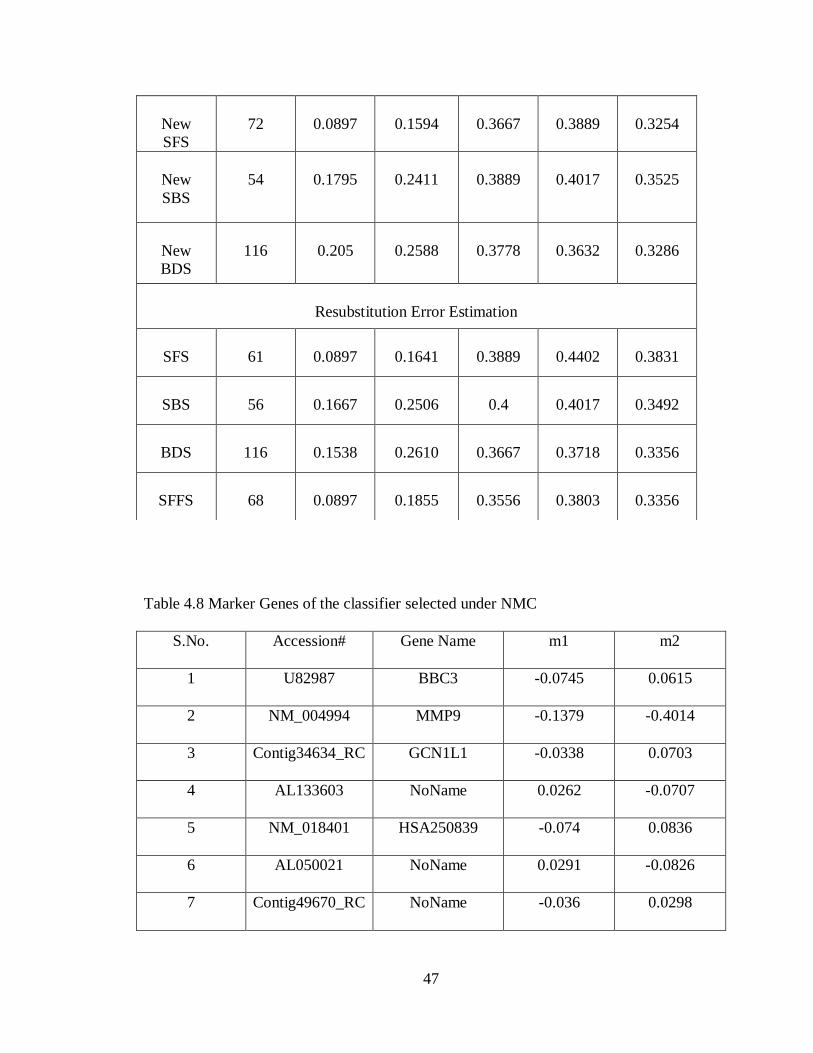
47

Table 4.8 Marker Genes of the classifier selected under NMC

S.No. Accession# Gene Name m1 m2

1 U82987 BBC3 -0.0745 0.0615

2 NM_004994 MMP9 -0.1379 -0.4014

3 Contig34634_RC GCN1L1 -0.0338 0.0703

4 AL133603 NoName 0.0262 -0.0707

5 NM_018401 HSA250839 -0.074 0.0836

6 AL050021 NoName 0.0291 -0.0826

7 Contig49670_RC NoName -0.036 0.0298

New

SFS

72

0.0897

0.1594

0.3667

0.3889

0.3254

New

SBS

54

0.1795

0.2411

0.3889

0.4017

0.3525

New

BDS

116

0.205

0.2588

0.3778

0.3632

0.3286

Resubstitution Error Estimation

SFS

61

0.0897

0.1641

0.3889

0.4402

0.3831

SBS

56

0.1667

0.2506

0.4

0.4017

0.3492

BDS

116

0.1538

0.2610

0.3667

0.3718

0.3356

SFFS

68

0.0897

0.1855

0.3556

0.3803

0.3356

48

8 Contig51519_RC NoName 0.0419 -0.0617

9 AF201951 CFFM4 -0.1578 0.031

10 AB032973 LCHN 0.0026 -0.0771

11 NM_003748 ALDH4 -0.1102 0.1235

12 NM_016448 L2DTL 0.0597 -0.134

13 Contig53268_RC FLJ12150 -0.0746 0.055

14 Contig46653_RC NoName -0.0565 -0.1821

15 AL137514 NoName -0.1053 0.0198

16 Contig25343_RC NoName 0.0763 -0.0429

17 NM_003882 WISP1 -0.1321 0.0597

18 NM_002019 FLT1 0.0158 -0.0926

19 AF257175 NoName -0.0611 0.0825

20 Contig53742_RC NoName -0.1057 0.0328

21 AB033007 KIAA1181 0.0239 0.1303

22 NM_013262 MIR -0.0568 0.0601

23 NM_001280 CIRBP -0.1102 0.0116

24 NM_018120 FLJ10511 -0.015 -0.1226

25 Contig32125_RC NoName -0.104 0.0541

26 NM_000436 OXCT 0.0433 -0.1001

27 Contig43747_RC NoName -0.0611 0.0408

28 Contig17359_RC NoName 0.0256 -0.051

29 NM_006117 PECI -0.0877 0.0555

30 AF055033 IGFBP5 -0.0012 -0.1664

49

31 Contig53646_RC NoName -0.1099 0.0205

32 Contig2399_RC SM-20 0.0234 -0.0841

33 NM_004911 ERP70 -0.0791 0.0387

34 X05610 COL4A2 0.0418 -0.0888

35 AL080110 NoName 0.0066 -0.0644

36 NM_015434 DKFZP434B168 0.0473 -0.0615

37 Contig25055_RC NoName -0.0782 0.0415

38 NM_018098 FLJ10461 0.0221 -0.132

39 Contig63102_RC FLJ11354 -0.0941 0.0409

40 AF052162 FLJ12443 -0.0048 -0.1868

41 AB037863 KIAA1442 -0.1302 0.0633

42 NM_003607 PK428 0.0336 -0.1074

43 Contig55377_RC NoName -0.0964 0.0507

44 NM_006265 RAD21 0.0096 -0.1509

45 Contig46223_RC NoName -0.074 0.0689

46 Contig42421_RC NoName -0.1056 0.0528

47 NM_000286 PEX12 0.0085 0.131

48 NM_006281 STK3 0.0172 -0.0918

49 Contig57595 NoName -0.1859 0.0506

50 AB020689 KIAA0882 -0.3066 -0.0272

51 NM_000017 ACADS -0.0799 0.0676

52 NM_000224 KRT18 -0.2112 -0.0113

53 NM_015416 DKFZP586A011 -0.0678 0.0296

50

54 Contig55813_RC NoName -0.0694 0.0305

55 NM_001282 AP2B1 -0.0787 0.0568

56 AA555029_RC NoName 0.0159 -0.1279

57 NM_004480 FUT8 -0.0762 0.0364

58 AL137295 NoName 0.0254 -0.0569

59 AF148505 MMSDH -0.0658 0.0683

60 AF052159 NoName 0.0211 -0.0813

61 NM_000320 QDPR -0.1848 0.0116

62 NM_000599 IGFBP5 -0.0629 -0.2541

63 AB033043 DKFZP761L0424 -0.061 0.0474

64 NM_003234 TFRC -0.0423 -0.1935

65 Contig41887_RC NoName -0.2376 -0.0059

66 NM_004603 STX1A -0.0793 -0.2084

67 NM_004798 KIF3B 0.0116 0.111

68 Contig21812_RC FLJ21924 0.0571 -0.0257

69 Contig3902_RC NoName 0.0346 -0.0617

70 NM_000158 GBE1 0.02 -0.0915

71 U58033 MTMR2 0.0531 -0.0524

72 M21551 NMB 0.0193 -0.0969

4.2.3. Conclusion of results obtained by training 231 genes

Table 4.9 shows a summary of the performance of the best LDA, QDA, SVM and

NM classifiers trained from first data set. From bootstrap error estimation values NM and

51

SVM classifiers perform better than LDA and QDA. We think that the NM classifier

performs good because it is very simple and in the applications such as the problem in

this thesis is less prone to the curse of dimensionality (Edward R. Dougherty 2005-04).

The SVM performs well because it does not assume Gaussian distributions for the feature

sets under each class. From these results, we may observe that the Gaussian is not a good

approximate for gene expression value distribution.

In order to compare our classifiers to the classifier presented in (Van‟t Veer LJ 2002),

we have evaluated its performance on all three data sets and the results are reported in

Table 4.10. In Table 4.10, the first three columns give the leave one out error estimation,

resubstitution error estimation and bootstrap error estimation results for the first data set.

The columns four, five and six give the hold out error rates for paper (Van de Vijver MJ

2002)data. The paper (Van de Vijver MJ 2002) data has been used considering three

different cases. The first case is the new node negative patients, second is the all the new

patients and the third case is the all the new and old patients. The last column in this table

gives the hold out error for the third data set. In this section will not use this error as the

231 expression values are not presented in this data set. Upon comparison we can see that

all the classifiers we have obtained have better results with the bootstrap error estimation

and their performance on the second data set. Specially, the NM classifier shows

significant improvement. Considering that NM classifier is as simple as the classifier

used in (Van‟t Veer LJ 2002), we guess that the improvement is the result of a better

feature selection algorithm.

52

Table 4.9 Conclusion of the results obtained by training and validating 231 genes from

paper (Van‟t Veer LJ 2002)

Number of

Marker

Genes

Training

Error

Bootstrap

Error

Estimation

Error based on paper [2] data

New Node

Negative

Patients

ALL New

Patients

ALL

Patients

(New and

Old)

LDA

SFS

Resub

39

0

0.2371

0.3889

0.4145

0.3458

QDA

SFS

LOO

49

0.0769

0.2564

0.3480

0.3676

0.3390

SVM

SBS

LOO

58

0.0128

0.1690

0.3889

0.4274

0.3525

NMC

New

SFS

LOO

72

0.0897

0.1594

0.3667

0.3889

0.3254

Table 4.10 Summary of results obtained by using classifier (Van‟t Veer LJ 2002)

(Van‟t Veer LJ 2002) data

(Van de Vijver MJ 2002)

data

(Marc Buyse

and Annuska

M. Glas

2006)data

Leave One

Out

Error

Resubstit

ution

Error

Bootstrap

Error

Estimate

New Node

Negative

Patients (90)

All New

Patients

(234)

All

Patients

(295)

New Test data

with 307

patients

0.3077

0.2692

0.3099

0.4

0.4145

0.3831

0.4365

53

4.2.4. Training of Classification Algorithms with the given 70 Gene Expressions

In this section we re-trained LDA, QDA, SVM and NMC classifiers starting with the

70 marker genes reported in (Van‟t Veer LJ 2002). The main aim of this re-

implementation is to have the ability to evaluate the performance of our classifiers on the

third data set and compare them with the performance of the classifier in (Van‟t Veer LJ

2002).

Table 4.11 shows the results of training and validation for different classifiers

obtained by using LDA classification rule with different gene selection methods and

different error estimation algorithms. This table is similar to the previous tables, except it

has an additional column which shows the error rate when the classifier is applied to third

data set.

Upon comparing the results from table 4.11, it can be seen that, here the bootstrap

error estimation results among different feature selection and error estimation errors are

not that much different and this even true with the validation results as well. The

minimum bootstrap error in this table is 0.1158 which is obtained by backward selection

algorithm with leave one out error estimation. But, when this classifier is applied to the

data set (Marc Buyse and Annuska M. Glas 2006)the error rate is very high and hence

this classifier cannot be the best. Therefore we choose a classifier which has better

validation results. In the table, we can see the classifier with floating point forward

selection and resubstitution error estimation has a bootstrap error rate of 0.2672. This

classifier has a training error of 0.1923 with 28 marker genes. The error when we apply

this classifier to the data set in paper (Marc Buyse and Annuska M. Glas 2006) we get

0.4625. Even though the bootstrap error rate is high, the validation results of this

54

classifier are better than other classifiers. Hence this classifier is considered as the best in

this table. In this category, the classifier selection should is done on the basis of both

bootstrap error estimation and the performance of it with paper (Marc Buyse and

Annuska M. Glas 2006) data.

Table 4.12 presents the results obtained by training the 70 marker genes using QDA

classification rule. From the table it can be seen that, the minimum bootstrap error in this

table is 0.2455 which is obtained by bidirectional selection with leave one out error

estimation. But when the classifier is applied to data in (Marc Buyse and Annuska M.

Glas 2006) the result is not satisfactory. Hence this cannot be the best classifier in this

table. Here we need to consider both the Bootsrap error estimation and validation results

to select the best classifier. The classifier with forward selection and resubstitution error

estimation has bootstrap error of 0.2607. It has a training error of 0 with 42 marker genes.

When we apply this classifier to the data set in paper (Marc Buyse and Annuska M. Glas

2006) we obtain an error rate of 0. 4332. Hence this classifier can be considered as the

best in this table.

Table 4.13 presents the results obtained by implementing SVM as a classification

rule. On comparing the results in this table, it can be seen that we have obtained very low

bootstrap error rates but the classifiers when applied to paper (Marc Buyse and Annuska

M. Glas 2006) data yielded very high error rates. The classifier with enhanced backward

selection and leave one out error estimation has a bootstrap error estimate of 0.1050. It

has a training error of 0 with 36 marker genes. The error rate obtained when this classifier

is applied to the data set from (Marc Buyse and Annuska M. Glas 2006) is 0.4951. Even

55

though all the results are very high, but this classifier has the lowest error rates in this

table.

Table 4.14 presents the results obtained by implementing the Nearest mean

classification rule. On comparing the results, the bootstrap error rates among different

feature selection and error estimation errors is not that much different and the validation

results are not very different. The minimum bootstrap error estimate in this table is

0.1435 and it is obtained by forward selection with resubstitution error estimate classifier.

But when this classifier is applied to the data in paper (Marc Buyse and Annuska M.

Glas 2006) the error rate is very high. Hence this classifier cannot be considered as the

best in this table. The classifier with forward selection and leave one out error estimation

has a bootstrap error is 0.1608. It has a training error of 0.1026 with 42 marker genes.

The error rate obtained when this classifier is applied to the paper (Marc Buyse and

Annuska M. Glas 2006) is 0.4495. Since these results are the lowest we obtained in this

table, this classifier can be considered as the best.

56

Table 4.11 Results Obtained by training a LDA classifier on 70 features from data set

(Van‟t Veer LJ 2002)

Feature

Selection

Methods

Number of

Marker

Genes

Training

Error

Bootstrap Error

Estimation

Error based

on new paper

data

New Test

data

(307)

SFS

31

0.141

0.2374

0.5016

SBS

30

0.0385

0.1158

0.4984

BDS

35

0.1785

0.2111

0.5147

SFFS

33

0.0513

0.1827

0.4919

New

SFS

30

0.05128

0.1507

0.5081

New

SBS

36

0.0128

0.1162

0.4756

New

BDS

34

0.1026

0.2636

0.4853

Resubstitution Error Estimation

SFS

30

0

0.1562

0.5309

SBS

20

0.2064

0.2433

0.5016

BDS

35

0.1410

0.2625

0.4691

SFFS

28

0.1923

0.2672

0.4625

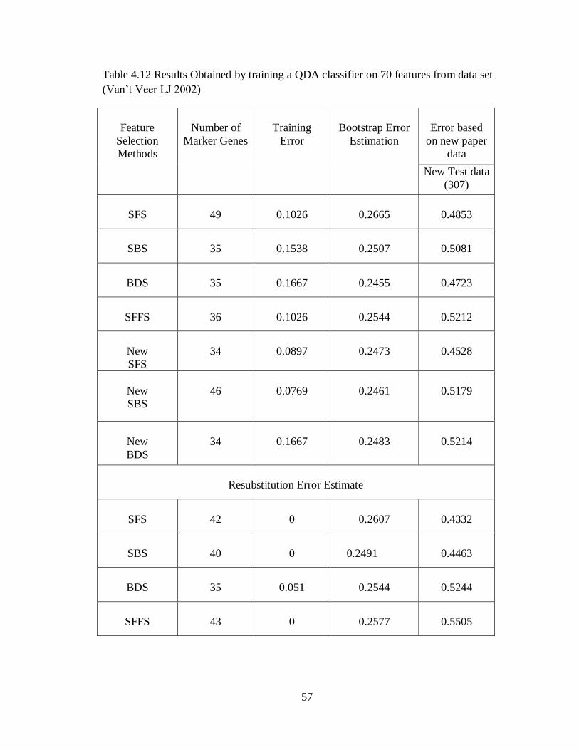
57

Table 4.12 Results Obtained by training a QDA classifier on 70 features from data set

(Van‟t Veer LJ 2002)

Feature

Selection

Methods

Number of

Marker Genes

Training

Error

Bootstrap Error

Estimation

Error based

on new paper

data

New Test data

(307)

SFS

49

0.1026

0.2665

0.4853

SBS

35

0.1538

0.2507

0.5081

BDS

35

0.1667

0.2455

0.4723

SFFS

36

0.1026

0.2544

0.5212

New

SFS

34

0.0897

0.2473

0.4528

New

SBS

46

0.0769

0.2461

0.5179

New

BDS

34

0.1667

0.2483

0.5214

Resubstitution Error Estimate

SFS

42

0

0.2607

0.4332

SBS

40

0

0.2491

0.4463

BDS

35

0.051

0.2544

0.5244

SFFS

43

0

0.2577

0.5505

58

Table 4.13 Results Obtained by training a SVM classifier on 70 features from data set

(Van‟t Veer LJ 2002)

Feature

Selection

Methods

Number of

Marker Genes

Training Error

Bootstrap Error

Estimation

Error based

on new

paper(Marc

Buyse and

Annuska M.

Glas 2006)

data

New Test data

(307)

SFS

40

0.0897

0.1558

0.5016

SBS

26

0

0.1076

0.4691

BDS

35

0.1538

0.1383

0.5179

SFFS

43

0.038

0.1580

0.5244

New

SFS

40

0.038

0.1168

0.5179

New

SBS

36

0

0.1050

0.4951

New

BDS

34

0.064

0.1907

0.5214

Resubstitution Error Estimate

SFS

21

0

0.1884

0.5114

SBS

25

0

0.1821

0.5472

59

BDS

35

0

0.1176

0.5114

SFFS

19

0

0.1682

0.5210

Table 4.14 Results Obtained by training a NMC classifier on 70 features from data set

(Van‟t Veer LJ 2002)

Feature

Selection

Methods

Number of

Marker

Genes

Training

Error

Bootstrap Error

Estimation

Error based

on new paper

data

New Test

data

(307)

SFS

42

0.1026

0.1608

0.4495

SBS

33

0.1667

0.2408

0.4625

BDS

35

0.1528

0.2461

0.4756

SFFS

46

0.1154

0.1825

0.4495

New

SFS

52

0.1154

0.1702

0.4560

New

SBS

40

0.141

0.2045

0.4528

New

BDS

34

0.1538

0.2770

0.4619

Resubstitution Error Estimation

SFS

22

0.1282

0.1435

0.4658

60

SBS

19

0.141

0.2053

0.4886

BDS

35

0.1282

0.2302

0.4821

SFFS

20

0.0769

0.1712

0.4723

4.2.5. Conclusion of the results obtained by implementing 70 genes

Table 4.15 shows the classifiers under each classification rule which have obtained

the best results. In this section we will the pick the best classifier under this category. The

selection of the best classifier is based on the comparison of the bootstrap results and the

validation results of each classifier with the paper (Marc Buyse and Annuska M. Glas

2006) data. Upon comparison it can be seen that NM and SVM classifiers performed

better than LDA and QDA. Even though QDA classifier looks good with the lowest

validation result in the table, it cannot be the best due to high bootstrap. Therefore in

between NM and SVM, Nearest mean can be chosen as the best because of lower

validation result than SVM. Hence this classifier can be considered as the best in this

category

61

Table 4.15 Conclusion of the results obtained by training and validating 70 genes from

Paper (Van‟t Veer LJ 2002)

Number of

Marker

Genes

Training

Error

Bootstrap Error

Estimation

Error based on

new paper data

New Test data

(307)

LDA

SFFS

RESUB

28

0.1923

0.2672

0.4625

QDA

SFS

RESUB

42

0

0.2607

0.4332

SVM

NEW

SBS

LOO

36

0

0.1050

0.4951

NMC

SFS

LOO

42

0.1026

0.1608

0.4495

4.3. Classifier with the combined data sets from (Van‟t Veer LJ 2002) and (Van de Vijver

MJ 2002)

In this section, we combined the data sets from sources (Van‟t Veer LJ 2002) and

(Van de Vijver MJ 2002) to form 312 patient data. The main idea of combining the data

was to check if there is any improvement in the bootstrap error estimate of the classifiers.

Initially we trained these 312 patient‟s data with different classification algorithms

presented in section 4.2 and then we evaluated the bootstrap algorithm on the optimum

subset.

Table 4.16 shows the results for LDA classification rule with different gene selection

methods and different error estimation algorithms. The table is similar to the previous

62

tables with the first column with the number of genes, second column with the training

error, third column with the bootstrap error rate. Upon comparing the results presented in

table 4.16, it can be seen that the minimum bootstrap error is 0.2005 which is obtained by

backward selection with leave one out error estimation. The training error of this

classifier is 0.1282 with 75 marker genes. Since this is the lowest error we achieved in

this table. Hence, this classifier can be selected as the best in this section.

Table 4.17 presents the results obtained by implementing QDA classification rule.

Upon comparing the results in this table, it can be seen that the minimum bootstrap error

obtained in this table is 0.2041 which is obtained by sequential floating point forward

selection with leave one out error estimation classifier. The training error obtained is

0.1378 with 42 marker genes. Since this is the lowest error rate obtained in this table this

classifier can be considered as the best.

Table 4.18 shows the results for SVM classification rule with different gene selection

methods and different error estimation algorithms. On comparing the results presented in

this table, the minimum bootstrap error is 0.2932 which is obtained by enhanced

backward selection with leave one out error estimation classifier. This classifier has

obtained a training error of 0.2612 with 62 marker genes. The bootstrap error obtained in

this method is high, but since this is the lowest in this table. Hence this classifier can be

selected as the best in this table.

Table 4.19 presents the results obtained by implementing the NM classification rules

with different feature selection methods and error estimation methods. Upon comparison

of the results presented in this table, the minimum bootstrap error is 0.1986 which is

obtained by floating point forward selection with resubstitution error estimation

63

classifier. The training error obtained by this classifier is 0.1812 with 55 marker genes.

Since this error rate is the lowest in this table, this classifier can be selected as the best.

4.3.1. Conclusion of the results obtained by implementing combined data sets (Van‟t

Veer LJ 2002) and (Van de Vijver MJ 2002)

Table 4.20 shows best results obtained by training and validating the combined data

set from papers (Van‟t Veer LJ 2002) and (Van de Vijver MJ 2002). In this section we

will pick one classifier which gives the best performance. As we think bootstrap error

estimation is the best tool for evaluating the performance of any classifier, hence the best

classifier should have a minimum bootstrap error. Upon comparison, all the classifiers in

the table 4.120 the minimum bootstrap error is 0.1986 which is obtained by NMC

classification rule with bidirectional selection and leave one out error estimation

classifier.

64

Table 4.16 Results Obtained by training a LDA classifier on 231 features from data sets

(Van‟t Veer LJ 2002) and (Van de Vijver MJ 2002)

Feature

Selection

Methods

Number of

Marker

Genes

Training

Error

Bootstrap

Error

Estimation

SFS

55

0.2949

0.3087

SBS

75

0.1282

0.2005

BDS

116

0.2596

0.3412

SFFS

52

0.2788

0.2987

New

SFS

62

0.2576

0.2954

New

SBS

64

0.2432

0.2763

New

BDS

116

0.2775

0.2983

Resubstitution Error Estimation

SFS

78

0.1635

0.3103

SBS

45

0.3118

0.3214

BDS

116

0.3421

0.3678

SFFS

35

0.2855

0.3137

65

Table 4.17: Results Obtained by training a QDA classifier on 231 features from data sets

(Van‟t Veer LJ 2002) and (Van de Vijver MJ 2002)

Feature

Selection

Methods

Number of

Marker

Genes

Training

Error

Bootstrap

Error

Estimation

SFS

59

0.2372

0.2115

SBS

45

0.2015

0.2080

BDS

116

0.3205

0.3628

SFFS

42

0.1378

0.2041

New

SFS

54

0.1795

0.2081

New

SBS

68

0.1985

0.2229

New

BDS

116

0.2196

0.2486

Resubstitution Error Estimation

SFS

31

0.1426

0.2145

SBS

59

0.1286

0.2218

BDS

116

0.2372

0.2980

SFFS

54

0.1426

0.2189

66

Table4.18: Results Obtained by training a SVM classifier on 231 features from data sets

(Van‟t Veer LJ 2002) and (Van de Vijver MJ 2002)

Feature

Selection

Methods

Number of

Marker

Genes

Training

Error

Bootstrap

Error

Estimation

SFS

72

0.2956

0.329

SBS

54

0.326

0.3443

BDS

116

0.2863

0.3254

SFFS

59

0.2996

0.3265

New

SFS

55

0.2887

0.3012

New

SBS

62

0.2612

0.2932

New

BDS

116

0.3221

0.3453

Resubstitution Error Estimation

SFS

52

0.2987

0.3245

SBS

65

0.3165

0.3543

BDS

116

0.3222

0.3467

SFFS

68

0.2897

0.3356

67

Table4.19: Results Obtained by training a NMC classifier on 231 features from data sets

(Van‟t Veer LJ 2002) and (Van de Vijver MJ 2002)

Feature Selection

Methods

Number of

Marker Genes

Training

Error

Bootstrap Error

Estimation

SFS

63

0.2756

0.3018

SBS

77

0.3077

0.3435

BDS

116

0.2949

0.3523

SFFS

65

0.2436

0.2947

New

SFS

74

0.2404

0.2879

New

SBS

62

0.2756

0.3157

New

BDS

68

0.2908

0.3322

Resubstitution Error Estimation

SFS

71

0.266

0.3047

SBS

72

0.2981

0.3355

BDS

116

0.2885

0.352

SFFS

55

0.1812

0.1986

68

Table 4.20: Conclusion of the results obtained by implementing combined data sets

(Van‟t Veer LJ 2002) and (Van de Vijver MJ 2002)

Number of

Marker Genes

Training Error

Bootstrap Error

Estimation

LDA

SBS

LOO

75

0.1282

0.2005

QDA

SFFS

LOO

42

0.1378

0.2041

SVM

NEW

SBS

LOO

62

0.2612

0.2932

NMC

SFFS

RESUB

55

0.1812

0.1986

4.4 Classifier with the combined data sets from (Van‟t Veer LJ 2002), (Van de Vijver MJ

2002) and (Marc Buyse and Annuska M. Glas 2006)

In this section we combined the data sets (Van‟t Veer LJ 2002), (Van de Vijver MJ

2002) and (Marc Buyse and Annuska M. Glas 2006) to form a 619 patient‟s data.

Initially we train this data using all classification algorithms discussed in section 4.2.

Then we will apply bootstrap error estimation to the obtained marker genes. The main

goal of re-implementing all the classification algorithms is to check if we can enhance the

performance of our classifiers.

Table 4.21 shows the results of training for LDA classification rule with different

gene selection methods and different error estimation algorithms. Upon comparing the

69

results presented in this table, we can see that the bootstrap error rates among different

feature selection and error estimation errors are not that much different. The minimum

bootstrap error is 0.3624 which is obtained by backward selection with resubstitution

error estimation classifier. The training error obtained by this classifier is 0.3275 with 27

marker genes. Since this classifier has the lowest bootstrap error it can be considered as

the best in this table.

Table 4.22 presents the results obtained by implementing QDA classification rule. On

comparing the results presented in this table, it can be seen that the minimum bootstrap

error in this table is 0.2491 which is obtained by floating point forward selection using

leave one out error estimation classifier. The training error obtained by this classifier is

0.2536 with 22 marker genes. Since this classifier has the minimum bootstrap error, this

classifier is selected as the best in this table.

Table 4.23 shows the results obtained by implementing SVM classification rule.

Upon comparing the results, it can be seen that the bootstrap error rates are not very

different. The minimum bootstrap error in this table is 0.2931 which is obtained by

enhanced backward selection with leave one out error estimation classifier. The training

error obtained by this classifier is 0.2543 with 29 marker genes. Hence this classifier can

be selected as the best in this table.

Table 4.24 presents the results obtained by implementing Nearest mean classification

rule with different feature selection methods and error estimation methods. On comparing

the results in this table, it can be seen that the minimum bootstrap error in this table is

0.3750 which is obtained by forward selection with resubstitution error estimation

70

classifier. The training error obtained by this classifier is 0.3053 with 22 marker genes.

Since this classifier has the minimum bootstrap in this table this is considered as the best.

4.4.1 Conclusion of the results obtained by implementing combined data sets (Van‟t Veer

LJ 2002), (Van de Vijver MJ 2002) and (Marc Buyse and Annuska M. Glas 2006)

Table 4.25 summarizes the results which we have picked as the best classifiers in the

section 4.4. From this table we will choose one classifier which is the best in this

category. In this table, the best classifier is the one which has minimum bootstrap error.

The classifier with QDA classification rule with floating point forward selection and

leave one out error estimation has the lowest bootstrap of 0.2491 and training error with

0.2536. Hence this classifier can be considered as the best in this category.

71

Table 4.21: Results Obtained by training a LDA classifier on 70 features from data sets

(Van‟t Veer LJ 2002), (Van de Vijver MJ 2002) and (Marc Buyse and Annuska M. Glas

2006)

Leave One Out Error Estimation

Feature Selection

Methods

Number of

Marker Genes

Training Error

Bootstrap

Error

Estimation

SFS

49

0.3166

0.3853

SBS

26

0.2876

0.3785

BDS

35

0.336

0.3720

SFFS

36

0.3102

0.3661

New

SFS

28

0.2956

0.3729

New

SBS

32

0.2375

0.3697

New

BDS

34

0.3118

0.3692

Resubstitution Error Estimation

SFS

65

0.2569

0.3727

SBS

27

0.3275

0.3624

BDS

35

0.3411

0.3862

72

SFFS

22

0.3767

0.3803

Table 4.22: Results Obtained by training a QDA classifier on 70 features from data sets

(Van‟t Veer LJ 2002), (Van de Vijver MJ 2002) and (Marc Buyse and Annuska M. Glas

2006)

Leave One Out Error Estimation

Feature Selection

Methods

Number of

Marker Genes

Training Error

Bootstrap

Error

Estimation

SFS

20

0.2666

0.2745

SBS

36

0.2553

0.2720

BDS

35

0.2795

0.2545

SFFS

22

0.2536

0.2491

New

SFS

34

0.2746

0.2832

New

SBS

40

0.2456

0.2693

New

BDS

34

0.2795

0.2891

Resubstitution Error Estimation

SFS

66

0.0468

0.2636

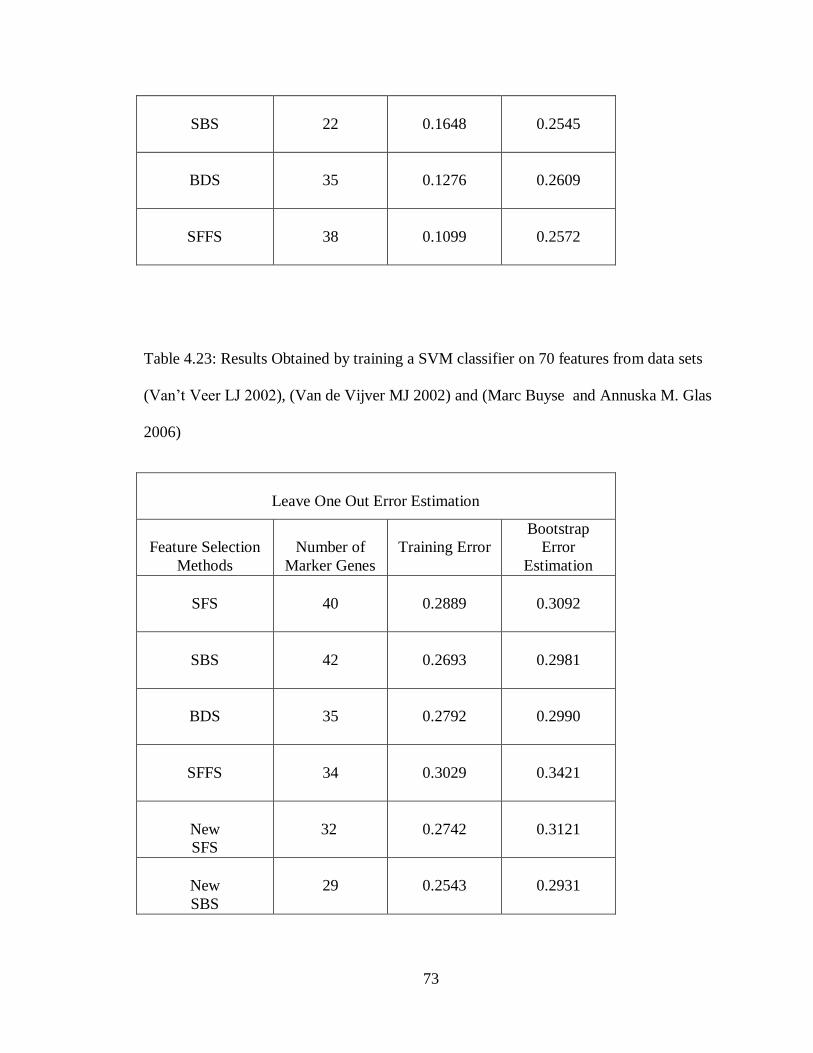
73

SBS

22

0.1648

0.2545

BDS

35

0.1276

0.2609

SFFS

38

0.1099

0.2572

Table 4.23: Results Obtained by training a SVM classifier on 70 features from data sets

(Van‟t Veer LJ 2002), (Van de Vijver MJ 2002) and (Marc Buyse and Annuska M. Glas

2006)

Leave One Out Error Estimation

Feature Selection

Methods

Number of

Marker Genes

Training Error

Bootstrap

Error

Estimation

SFS

40

0.2889

0.3092

SBS

42

0.2693

0.2981

BDS

35

0.2792

0.2990

SFFS

34

0.3029

0.3421

New

SFS

32

0.2742

0.3121

New

SBS

29

0.2543

0.2931

74

New

BDS

35

0.2654

0.3134

Resubstitution Error Estimation

SFS

52

0.2462

0.2933

SBS

26

0.3019

0.3338

BDS

35

0.2891

0.3412

SFFS

32

0.2990

0.3123

Table 4.24: Results Obtained by training a NMC classifier on 70 features from data sets

(Van‟t Veer LJ 2002), (Van de Vijver MJ 2002) and (Marc Buyse and Annuska M. Glas

2006)

Leave One Out Error Estimation

Feature Selection

Methods

Number of

Marker Genes

Training Error

Bootstrap

Error

Estimation

SFS

34

0.3069

0.3821

SBS

32

0.3279

0.4133

BDS

36

0.3312

0.4108

75

SFFS

19

0.3029

0.3959

New

SFS

36

0.2569

0.4019

New

SBS

30

0.2601

0.4084

New

BDS

34

0.2779

0.3971

Resubstitution Error Estimation

SFS

22

0.3053

0.3750

SBS

35

0.3312

0.4160

BDS

35

0.3296

0.4214

SFFS

27

0.294

0.3905

4.25 Conclusion of the results obtained by training and validating data from papers

(Van‟t Veer LJ 2002), (Van de Vijver MJ 2002) and (Marc Buyse and Annuska M. Glas

2006)

Number of Marker

Genes

Training Error

Bootstrap Error

Estimation

LDA

SBS

RESUB

27

0.3275

0.3624

QDA

SFFS

LOO

22

0.2536

0.2491

76

SVM

NEW

SBS

LOO

29

0.2543

0.2931

NMC

SFS

RESUB

22

0.3053

0.3750

77

CHAPTER 5

CONCLUSION AND FUTURE SCOPE

The main goal of this thesis is to predict the outcome of a breast cancer tumor in early

stages based on the data received from micro-array analysis of tumor cells. The result of

this prognosis helps physicians to form an educated decision on the treatment needed for

patient. While the classifier presented in (Van‟t Veer LJ 2002), showed the capability of

micro-array analysis in this regard, the statistical methods used to design the classifier

can be improved to get a better prognosis tool. In this thesis, we applied different

statistical tools especially various classification algorithms, different feature selection

methods, and variety of error estimation tools to this problem and searched for a classifier

with lowest probability of error. We used Linear discriminant Analysis (LDA), Quadratic

discriminant analysis (QDA), Support Vector Machines (SVM) and Nearest Mean

Classifier (NMC) as classification rules. We used four different types of feature selection

methods. Likewise, we designed a new method of feature selection by making some

enhancements to the traditional methods. We also used three different error estimation

methods. Then we evaluated the performance of the classifiers we have designed and

compared them with each other and with the classifier presented in (Van‟t Veer LJ 2002).

The best classifier we obtained in this thesis is the Nearest mean classifier which has

obtained a very low bootstrap error. Here is the summary of important finding of this

effort:

- Simple classifiers such as NMC perform better for this problem than classifiers

with higher complexity.

78

- Gaussian distribution is not a good approximation for the distribution of the

micro-array data, therefore LDA and QDA classifiers perform worse than

classifiers such as SVM.

- There is not a significant difference in the suboptimal feature search algorithms

such as forward or backward selection algorithms for this problem.

- The nearest mean classifier with floating forward selection with resubstitution

error estimation is the best among the classifiers we checked for this problem

which is obtained by combining data from (Van‟t Veer LJ 2002) and (Van de

Vijver MJ 2002)

This work can continue in two directions. First, one can try to enhance the error rates

by designing new classifiers using other classification rules, feature selection methods

and error estimation algorithms. The second direction is focusing on Nyman-Pearson type

classifiers and instead of minimizing the overall error, design classifiers that minimize

the false positive while keeping the false negative below a threshold.

79

REFERENCES

[1] Anil Jain, D. Z. (1997). Feature Selection: Evaluation, Application, and Small Sample

Performance. IEEE Transactions on Pattern Analysis and Machine Intelligence. Volume

19: 153 - 158.

[2] Aniruddha Datta, E. R. D., Ed. (2007). Introduction to genomic signal processing with

control, CRC Press.

[3] Babu, M. M. An Introduction to Microarray Data Analysis.

[4] Bradley Efron, R. T. (1997). "Improvements on cross-validation: the .632+ bootstrap

method." Journal of the American Statistical Association Vol. 92: 548-560.

[5] BURGES, C. J. C. (1998). A Tutorial on Support Vector Machines for Pattern

Recognition. U. Fayyad. Boston, Bell Laboratories, Lucent Technologies.

[6] Chih-Wei Hsu, C.-C. C., and Chih-Jen Lin (2010). A Practical Guide to Support

Vector Classification. Taipei, Taiwan, National Taiwan University.

[7] Desheng Huang, Y. Q., Miao He, and Baosen Zhou (2009, 28(1): 149). "Comparison

of linear discriminant analysis methods for the classification of cancer based on gene

expression data." J Exp Clin Cancer Res.

[8] Edward R. Dougherty, I. S., Jie Chen, Z. Jane Wang, Ed. (2005-04). Genomic Signal

Processing and Statistics (Eurasip Book Series on Signal Processing and

Communications), Hindawi Publishing Corporation.

[9] Efron, B., Ed. (1982). The Jackknife, the Bootstrap and Other Resampling Plans

(CBMS-NSF Regional Conference Series in Applied Mathematics). Philadelphia, Pa,

USA, Society for Industrial Mathematics.

[10] Efron, B. (1983). "Estimating the error rate of a prediction rule: improvement on

cross-validation." Journal of the American Statistical Association Vol. 78 316-331.

[11] Gutierrez-Osuna, R. Introduction to Pattern Analysis, Texas A&M University.

[12] Iñaki Inza , B. S., Rosa Blanco , Pedro Larrañaga (2002). "Gene Selection By

Sequential Search Wrapper Approaches in Microarray Cancer Class Prediction." Journal

of Intelligent and Fuzzy Systems vol. 12: 25–34.

[13] Izenman, A. J. (1991). "Recent developments in nonparametric density estimation,."

J. Amer. Statist. Assoc vol. 86, no. 413, : pp. 205–224,.

80

[14] Kay, S. M., Ed. (1993). Fundamentals of Statistical Signal Processing Volume 2:

Detection Theory Prentice Hall PTR.

[15] Kronmal, P. W. W. a. R. A. (1977). "Discriminant functions when covariances are

unequal and sample sizes are moderate." International Biometric Society. vol. 33: 479–

484.

[16] Lin, C.-J. ( 2007). Support Vector Machines. National Taiwan University

[17] Marc Buyse , S. L., Laura van‟t Veer , Giuseppe Viale , Mauro Delorenzi , and e. A.

Annuska M. Glas (2006). "Validation and Clinical Utility of a 70-Gene Prognostic

Signature for Women With Node-Negative Breast Cancer; J Natl Cancer Inst ": 98: 1183

– 1192.

[18] Roy D. Yates, D. G., Ed. (May 2004, ©2005). Probability and Stochastic Processes:

A Friendly Introduction for Electrical and Computer Engineers.

[19] S. Balakrishnama, A. G. LINEAR DISCRIMINANT ANALYSIS - A BRIEF

TUTORIAL. Simrall, Hardy Rd., Mississippi, Institute for Signal and Information

Processing, Mississippi State University.

[20] Saeed, A. I. Introduction to Microarray Data Analysis and MeV, Pathogen

Functional Genomics Resource Center/ The Institute for Genomic Research.

[21] Shawe-Taylor, N. C. a. J., Ed. (2000). An introduction to support Vector Machines:

and other kernel-based learning methods. New York, NY, USA, Cambridge University

Press.

[22] Smola, B. S. a. A. J., Ed. (2002). Learning with Kernels - Support Vector Machines,

Regularization, Optimization, and Beyond, MIT Press.

[23] Teknomo, K. "Discriminant Analysis Tutorial." from.

http://people.revoledu.com/kardi/tutorial/LDA/

[24] Ultsch, A. Is log ratio a good value for identifying differential expressed genes in

microarray experiments? Marburg, Germany, University of Marburg.

[25] Van de Vijver MJ, H. Y., van‟t Veer LJ, Dai H, Hart AA, Voskuil DW, et al. (2002).

A gene-expression signature as a predictor of survival in breast cancer N Engl J Med:

347 : 1999 – 2009.

[26] Van‟t Veer LJ, D. H., van de Vijver MJ, et al. (2002). Gene expression profiling

predicts clinical outcome of breast cancer: 415:530-416.

[27] Vapnik, V. N., Ed. (1998). Statistical Learning Theory. New York, NY, USA,

JohnWiley & Sons.

81

[28] Walker, M. S. a. G. DNA Microarray Technology. What is it and how is it useful?

Cambridge, MA, Massachusetts Institute of Technology.

[29] Wettenhall, J., Linear Models in Microarrays: An Introduction.

[30] Wendy L. Martinez, A.R.M.,ed. Computational Statistics Handbook with MATLAB

1ed. 2001, Chapman & Hall.

[31] Stone, M., Cross-Validatory Choice and Assessment of Statistical Predictions.

Journal of the Royal Statistical Society, 1974. Vol. 36: p. 111-147.

[32] Richard Simon, M.D.R., Kevin Dobbin and Lisa M. McShane, Pitfalls in the Use of

DNA Microarray Data for Diagnostic and Prognostic Classification. J Natl Cancer Inst,

2003. 95(1): p. 14-18.

[33] Isabelle Guyon, C., Embedded Methods. 2007.

[34] horsten Joachims (SVMLight), C.-C.C.a.C.-J.L., , Holger Froehlich, Gorden Jemwa,

Kiyoung Yang. The Spider. 2006; Available from:

http://www.kyb.tue.mpg.de/bs/people/spider/tutorial.html.

[35] Annette M. Molinaro, R.S., Ruth M. Pfeiffer, Prediction error estimation: a

comparison of resampling methods. Bioinformatics, 2005. Vol. 21: p. 3301-3307.

82

APPENDIX I

COVARIANCE MATRIX DATA OBTAINED BY LDA CLASSIFIER

Covariance matrix (C):

Columns 1 through 9

0.0857 0.0424 0.0064 0.0056 -0.0016 0.0043 0.0150 0.0091 0.0293

0.0424 0.2249 -0.0214 0.0218 0.1035 -0.0414 -0.0076 -0.0385 -0.0259

0.0064 -0.0214 0.0198 -0.0042 -0.0243 0.0124 0.0096 0.0090 0.0104

0.0056 0.0218 -0.0042 0.0518 0.0573 -0.0152 -0.0102 -0.0167 -0.0161

-0.0016 0.1035 -0.0243 0.0573 0.1964 -0.0455 -0.0280 -0.0448 -0.0508

0.0043 -0.0414 0.0124 -0.0152 -0.0455 0.0335 0.0125 0.0181 0.0227

0.0150 -0.0076 0.0096 -0.0102 -0.0280 0.0125 0.0230 0.0101 0.0187

0.0091 -0.0385 0.0090 -0.0167 -0.0448 0.0181 0.0101 0.0348 0.0263

0.0293 -0.0259 0.0104 -0.0161 -0.0508 0.0227 0.0187 0.0263 0.0736

0.0135 -0.0714 0.0180 -0.0385 -0.1161 0.0530 0.0215 0.0391 0.0397

0.0145 -0.0513 0.0094 -0.0294 -0.0718 0.0376 0.0148 0.0294 0.0307

0.0030 -0.0186 0.0185 0.0008 0.0015 0.0056 0.0077 0.0031 -0.0023

0.0088 -0.0185 0.0047 -0.0198 -0.0322 0.0165 0.0087 0.0152 0.0192

0.0596 0.0471 0.0088 0.0144 0.0106 0.0002 0.0137 -0.0050 0.0199

-0.0042 0.0359 -0.0137 0.0407 0.0909 -0.0232 -0.0183 -0.0209 -0.0370

0.0599 0.0266 0.0108 -0.0033 -0.0104 0.0110 0.0198 0.0080 0.0278

-0.0116 0.0271 -0.0055 0.0004 0.0324 -0.0084 -0.0032 -0.0073 -0.0151

0.0622 0.0387 0.0040 -0.0017 -0.0093 0.0135 0.0152 0.0043 0.0337

0.0079 -0.0121 0.0133 -0.0020 -0.0157 0.0090 0.0091 0.0048 0.0067

0.0212 0.0632 -0.0140 0.0374 0.0744 -0.0144 -0.0129 -0.0187 -0.0207

-0.0041 0.0346 -0.0087 0.0120 0.0489 -0.0160 -0.0089 -0.0192 -0.0243

-0.0021 0.0183 -0.0036 0.0147 0.0274 -0.0075 0.0001 -0.0072 -0.0057

-0.0029 0.0419 -0.0084 0.0137 0.0447 -0.0174 -0.0069 -0.0182 -0.0108

83

-0.0070 0.0145 -0.0069 0.0227 0.0433 -0.0113 -0.0090 -0.0133 -0.0230

-0.0134 0.0250 -0.0081 0.0286 0.0441 -0.0162 -0.0087 -0.0150 -0.0196

-0.0080 0.0236 -0.0129 0.0238 0.0619 -0.0178 -0.0134 -0.0104 -0.0271

0.0195 -0.0495 0.0123 -0.0175 -0.0722 0.0362 0.0108 0.0260 0.0233

0.0082 0.0140 0.0007 0.0026 0.0104 -0.0097 -0.0019 -0.0020 0.0025

0.0055 0.0156 -0.0027 0.0368 0.0542 -0.0130 -0.0195 -0.0124 -0.0368

0.0500 0.0481 0.0011 0.0101 0.0115 -0.0048 0.0116 -0.0065 0.0215

-0.0262 0.0140 -0.0059 -0.0057 0.0231 -0.0073 -0.0080 -0.0149 -0.0158

0.0091 -0.0069 -0.0005 -0.0046 -0.0245 0.0003 0.0016 0.0094 0.0197

0.0512 0.0261 0.0051 -0.0121 -0.0200 0.0117 0.0184 0.0100 0.0411

0.0123 -0.0155 0.0011 -0.0259 -0.0481 0.0143 0.0125 0.0155 0.0260

0.0186 -0.0212 0.0059 -0.0236 -0.0525 0.0173 0.0106 0.0142 0.0266

0.0220 -0.0001 0.0095 -0.0210 -0.0532 0.0227 0.0182 0.0124 0.0352

0.0037 -0.0147 0.0039 -0.0115 -0.0270 0.0111 0.0073 0.0125 0.0150

-0.0124 -0.0124 0.0041 -0.0099 -0.0103 0.0062 0.0056 0.0047 0.0033

0.0028 0.0196 -0.0062 0.0045 0.0276 -0.0064 -0.0041 -0.0104 -0.0036

Columns 10 through 18

0.0135 0.0145 0.0030 0.0088 0.0596 -0.0042 0.0599 -0.0116 0.0622

-0.0714 -0.0513 -0.0186 -0.0185 0.0471 0.0359 0.0266 0.0271 0.0387

0.0180 0.0094 0.0185 0.0047 0.0088 -0.0137 0.0108 -0.0055 0.0040

-0.0385 -0.0294 0.0008 -0.0198 0.0144 0.0407 -0.0033 0.0004 -0.0017

-0.1161 -0.0718 0.0015 -0.0322 0.0106 0.0909 -0.0104 0.0324 -0.0093

0.0530 0.0376 0.0056 0.0165 0.0002 -0.0232 0.0110 -0.0084 0.0135

0.0215 0.0148 0.0077 0.0087 0.0137 -0.0183 0.0198 -0.0032 0.0152

0.0391 0.0294 0.0031 0.0152 -0.0050 -0.0209 0.0080 -0.0073 0.0043

0.0397 0.0307 -0.0023 0.0192 0.0199 -0.0370 0.0278 -0.0151 0.0337

0.1573 0.0796 -0.0050 0.0363 -0.0001 -0.0587 0.0268 -0.0209 0.0267

84

0.0796 0.1150 -0.0135 0.0289 -0.0070 -0.0403 0.0175 -0.0100 0.0205

-0.0050 -0.0135 0.0653 -0.0075 0.0117 0.0070 0.0118 -0.0079 -0.0014

0.0363 0.0289 -0.0075 0.0390 -0.0091 -0.0287 -0.0002 0.0014 0.0110

-0.0001 -0.0070 0.0117 -0.0091 0.0711 -0.0019 0.0619 -0.0109 0.0560

-0.0587 -0.0403 0.0070 -0.0287 -0.0019 0.1079 -0.0089 0.0094 -0.0172

0.0268 0.0175 0.0118 -0.0002 0.0619 -0.0089 0.0917 -0.0100 0.0631

-0.0209 -0.0100 -0.0079 0.0014 -0.0109 0.0094 -0.0100 0.0260 -0.0140

0.0267 0.0205 -0.0014 0.0110 0.0560 -0.0172 0.0631 -0.0140 0.0948

0.0092 0.0061 0.0194 0.0046 0.0083 -0.0075 0.0097 -0.0050 0.0064

-0.0305 -0.0359 -0.0021 -0.0179 0.0179 0.0616 0.0038 0.0015 0.0207

-0.0451 -0.0283 0.0017 -0.0151 0.0065 0.0407 0.0097 0.0135 0.0019

-0.0181 -0.0132 -0.0017 -0.0068 0.0028 0.0104 -0.0028 0.0045 -0.0039

-0.0378 -0.0260 -0.0003 -0.0213 0.0084 0.0248 0.0071 0.0045 0.0032

-0.0329 -0.0281 -0.0006 -0.0098 -0.0038 0.0282 -0.0110 0.0105 -0.0120

-0.0333 -0.0293 -0.0011 -0.0111 -0.0004 0.0302 -0.0170 0.0047 -0.0093

-0.0342 -0.0230 0.0022 -0.0231 -0.0024 0.0506 -0.0076 0.0043 -0.0175

0.0920 0.0561 -0.0041 0.0251 0.0018 -0.0395 0.0121 -0.0221 0.0190

-0.0122 -0.0162 0.0037 0.0028 0.0058 0.0006 0.0006 -0.0005 0.0026

-0.0380 -0.0367 0.0092 -0.0221 0.0042 0.0641 -0.0130 -0.0025 -0.0084

-0.0041 -0.0040 -0.0061 -0.0090 0.0565 -0.0019 0.0646 -0.0033 0.0470

-0.0288 -0.0221 -0.0064 -0.0083 -0.0104 0.0109 -0.0119 0.0110 -0.0127

0.0086 0.0177 -0.0165 0.0089 0.0012 -0.0157 0.0111 -0.0042 0.0157

0.0300 0.0225 -0.0074 0.0126 0.0524 -0.0294 0.0775 -0.0086 0.0704

0.0460 0.0441 -0.0160 0.0177 0.0012 -0.0360 0.0326 -0.0046 0.0198

0.0460 0.0344 -0.0026 0.0198 0.0081 -0.0369 0.0185 -0.0131 0.0305

0.0577 0.0427 -0.0109 0.0141 0.0290 -0.0373 0.0520 -0.0054 0.0391

0.0240 0.0243 -0.0115 0.0110 -0.0028 -0.0219 0.0107 -0.0005 0.0064

85

0.0095 0.0118 0.0008 0.0075 -0.0120 -0.0133 -0.0085 0.0047 -0.0123

-0.0150 -0.0163 -0.0021 -0.0042 0.0060 0.0093 -0.0007 0.0033 0.0030

Columns 19 through 27

0.0079 0.0212 -0.0041 -0.0021 -0.0029 -0.0070 -0.0134 -0.0080 0.0195

-0.0121 0.0632 0.0346 0.0183 0.0419 0.0145 0.0250 0.0236 -0.0495

0.0133 -0.0140 -0.0087 -0.0036 -0.0084 -0.0069 -0.0081 -0.0129 0.0123

-0.0020 0.0374 0.0120 0.0147 0.0137 0.0227 0.0286 0.0238 -0.0175

-0.0157 0.0744 0.0489 0.0274 0.0447 0.0433 0.0441 0.0619 -0.0722

0.0090 -0.0144 -0.0160 -0.0075 -0.0174 -0.0113 -0.0162 -0.0178 0.0362

0.0091 -0.0129 -0.0089 0.0001 -0.0069 -0.0090 -0.0087 -0.0134 0.0108

0.0048 -0.0187 -0.0192 -0.0072 -0.0182 -0.0133 -0.0150 -0.0104 0.0260

0.0067 -0.0207 -0.0243 -0.0057 -0.0108 -0.0230 -0.0196 -0.0271 0.0233

0.0092 -0.0305 -0.0451 -0.0181 -0.0378 -0.0329 -0.0333 -0.0342 0.0920

0.0061 -0.0359 -0.0283 -0.0132 -0.0260 -0.0281 -0.0293 -0.0230 0.0561

0.0194 -0.0021 0.0017 -0.0017 -0.0003 -0.0006 -0.0011 0.0022 -0.0041

0.0046 -0.0179 -0.0151 -0.0068 -0.0213 -0.0098 -0.0111 -0.0231 0.0251

0.0083 0.0179 0.0065 0.0028 0.0084 -0.0038 -0.0004 -0.0024 0.0018

-0.0075 0.0616 0.0407 0.0104 0.0248 0.0282 0.0302 0.0506 -0.0395

0.0097 0.0038 0.0097 -0.0028 0.0071 -0.0110 -0.0170 -0.0076 0.0121

-0.0050 0.0015 0.0135 0.0045 0.0045 0.0105 0.0047 0.0043 -0.0221

0.0064 0.0207 0.0019 -0.0039 0.0032 -0.0120 -0.0093 -0.0175 0.0190

0.0169 -0.0069 -0.0044 0.0010 -0.0075 -0.0036 -0.0053 -0.0089 0.0093

-0.0069 0.0937 0.0234 0.0070 0.0094 0.0186 0.0326 0.0301 -0.0160

-0.0044 0.0234 0.0535 0.0042 0.0184 0.0164 0.0137 0.0076 -0.0389

0.0010 0.0070 0.0042 0.0170 0.0082 0.0061 0.0085 0.0071 -0.0100

-0.0075 0.0094 0.0184 0.0082 0.0455 0.0078 0.0110 0.0146 -0.0283

-0.0036 0.0186 0.0164 0.0061 0.0078 0.0328 0.0219 0.0202 -0.0228

86

-0.0053 0.0326 0.0137 0.0085 0.0110 0.0219 0.0490 0.0193 -0.0226

-0.0089 0.0301 0.0076 0.0071 0.0146 0.0202 0.0193 0.0829 -0.0168

0.0093 -0.0160 -0.0389 -0.0100 -0.0283 -0.0228 -0.0226 -0.0168 0.0967

0.0029 -0.0049 -0.0003 0.0075 -0.0018 0.0031 0.0024 0.0120 0.0033

-0.0009 0.0512 0.0189 0.0045 0.0032 0.0287 0.0293 0.0384 -0.0159

0.0020 0.0076 0.0089 0.0041 0.0114 0.0006 -0.0088 -0.0004 -0.0098

-0.0046 -0.0096 0.0175 0.0057 0.0157 0.0185 0.0107 0.0106 -0.0300

-0.0024 -0.0159 0.0017 -0.0046 -0.0022 -0.0001 -0.0026 -0.0029 0.0105

0.0047 -0.0107 -0.0035 -0.0033 0.0031 -0.0116 -0.0194 -0.0127 0.0197

-0.0011 -0.0324 -0.0161 -0.0081 -0.0074 -0.0208 -0.0294 -0.0229 0.0304

0.0049 -0.0140 -0.0149 -0.0105 -0.0155 -0.0223 -0.0202 -0.0278 0.0304

0.0037 -0.0341 -0.0116 -0.0073 -0.0052 -0.0131 -0.0227 -0.0198 0.0262

0.0006 -0.0169 -0.0053 -0.0038 -0.0117 -0.0105 -0.0164 -0.0199 0.0174

0.0051 -0.0132 -0.0029 0.0021 -0.0055 -0.0032 -0.0013 -0.0084 0.0031

-0.0049 0.0105 0.0111 0.0013 0.0129 0.0075 0.0066 0.0065 -0.0105

Columns 28 through 36

0.0082 0.0055 0.0500 -0.0262 0.0091 0.0512 0.0123 0.0186 0.0220

0.0140 0.0156 0.0481 0.0140 -0.0069 0.0261 -0.0155 -0.0212 -0.0001

0.0007 -0.0027 0.0011 -0.0059 -0.0005 0.0051 0.0011 0.0059 0.0095

0.0026 0.0368 0.0101 -0.0057 -0.0046 -0.0121 -0.0259 -0.0236 -0.0210

0.0104 0.0542 0.0115 0.0231 -0.0245 -0.0200 -0.0481 -0.0525 -0.0532

-0.0097 -0.0130 -0.0048 -0.0073 0.0003 0.0117 0.0143 0.0173 0.0227

-0.0019 -0.0195 0.0116 -0.0080 0.0016 0.0184 0.0125 0.0106 0.0182

-0.0020 -0.0124 -0.0065 -0.0149 0.0094 0.0100 0.0155 0.0142 0.0124

0.0025 -0.0368 0.0215 -0.0158 0.0197 0.0411 0.0260 0.0266 0.0352

-0.0122 -0.0380 -0.0041 -0.0288 0.0086 0.0300 0.0460 0.0460 0.0577

-0.0162 -0.0367 -0.0040 -0.0221 0.0177 0.0225 0.0441 0.0344 0.0427

87

0.0037 0.0092 -0.0061 -0.0064 -0.0165 -0.0074 -0.0160 -0.0026 -0.0109

0.0028 -0.0221 -0.0090 -0.0083 0.0089 0.0126 0.0177 0.0198 0.0141

0.0058 0.0042 0.0565 -0.0104 0.0012 0.0524 0.0012 0.0081 0.0290

0.0006 0.0641 -0.0019 0.0109 -0.0157 -0.0294 -0.0360 -0.0369 -0.0373

0.0006 -0.0130 0.0646 -0.0119 0.0111 0.0775 0.0326 0.0185 0.0520

-0.0005 -0.0025 -0.0033 0.0110 -0.0042 -0.0086 -0.0046 -0.0131 -0.0054

0.0026 -0.0084 0.0470 -0.0127 0.0157 0.0704 0.0198 0.0305 0.0391

0.0029 -0.0009 0.0020 -0.0046 -0.0024 0.0047 -0.0011 0.0049 0.0037

-0.0049 0.0512 0.0076 -0.0096 -0.0159 -0.0107 -0.0324 -0.0140 -0.0341

-0.0003 0.0189 0.0089 0.0175 0.0017 -0.0035 -0.0161 -0.0149 -0.0116

0.0075 0.0045 0.0041 0.0057 -0.0046 -0.0033 -0.0081 -0.0105 -0.0073

-0.0018 0.0032 0.0114 0.0157 -0.0022 0.0031 -0.0074 -0.0155 -0.0052

0.0031 0.0287 0.0006 0.0185 -0.0001 -0.0116 -0.0208 -0.0223 -0.0131

0.0024 0.0293 -0.0088 0.0107 -0.0026 -0.0194 -0.0294 -0.0202 -0.0227

0.0120 0.0384 -0.0004 0.0106 -0.0029 -0.0127 -0.0229 -0.0278 -0.0198

0.0033 -0.0159 -0.0098 -0.0300 0.0105 0.0197 0.0304 0.0304 0.0262

0.0473 -0.0007 0.0046 0.0113 0.0089 0.0103 -0.0004 0.0014 -0.0022

-0.0007 0.0930 -0.0104 0.0015 -0.0130 -0.0385 -0.0433 -0.0299 -0.0372

0.0046 -0.0104 0.0853 -0.0011 0.0121 0.0730 0.0258 0.0017 0.0525

0.0113 0.0015 -0.0011 0.0757 0.0033 -0.0030 -0.0135 -0.0124 -0.0026

0.0089 -0.0130 0.0121 0.0033 0.0595 0.0242 0.0249 0.0094 0.0280

0.0103 -0.0385 0.0730 -0.0030 0.0242 0.1222 0.0498 0.0262 0.0721

-0.0004 -0.0433 0.0258 -0.0135 0.0249 0.0498 0.0664 0.0218 0.0516

0.0014 -0.0299 0.0017 -0.0124 0.0094 0.0262 0.0218 0.0398 0.0262

-0.0022 -0.0372 0.0525 -0.0026 0.0280 0.0721 0.0516 0.0262 0.1055

-0.0059 -0.0151 0.0056 -0.0085 0.0065 0.0154 0.0222 0.0109 0.0226

0.0013 -0.0100 -0.0125 -0.0013 -0.0011 -0.0049 0.0026 0.0043 0.0043

88

-0.0023 0.0003 0.0070 0.0086 -0.0036 -0.0008 -0.0110 -0.0051 -0.0011

Columns 37 through 39

0.0037 -0.0124 0.0028

-0.0147 -0.0124 0.0196

0.0039 0.0041 -0.0062

-0.0115 -0.0099 0.0045

-0.0270 -0.0103 0.0276

0.0111 0.0062 -0.0064

0.0073 0.0056 -0.0041

0.0125 0.0047 -0.0104

0.0150 0.0033 -0.0036

0.0240 0.0095 -0.0150

0.0243 0.0118 -0.0163

-0.0115 0.0008 -0.0021

0.0110 0.0075 -0.0042

-0.0028 -0.0120 0.0060

-0.0219 -0.0133 0.0093

0.0107 -0.0085 -0.0007

-0.0005 0.0047 0.0033

0.0064 -0.0123 0.0030

0.0006 0.0051 -0.0049

-0.0169 -0.0132 0.0105

-0.0053 -0.0029 0.0111

-0.0038 0.0021 0.0013

-0.0117 -0.0055 0.0129

-0.0105 -0.0032 0.0075

-0.0164 -0.0013 0.0066

89

-0.0199 -0.0084 0.0065

0.0174 0.0031 -0.0105

-0.0059 0.0013 -0.0023

-0.0151 -0.0100 0.0003

0.0056 -0.0125 0.0070

-0.0085 -0.0013 0.0086

0.0065 -0.0011 -0.0036

0.0154 -0.0049 -0.0008

0.0222 0.0026 -0.0110

0.0109 0.0043 -0.0051

0.0226 0.0043 -0.0011

0.0330 0.0050 -0.0044

0.0050 0.0192 -0.0030

-0.0044 -0.0030 0.0216

90

APPENDIX – II

COVARIANCE MATRIX DATA OBTAINED BY QDA CLASSIFIER

Covariance (C1) of class 1

Columns 1 through 9

0.0166 0.0118 -0.0047 -0.0011 0.0268 0.0051 0.0102 0.0093 0.0041

0.0118 0.0308 -0.0027 0.0032 0.0438 0.0170 0.0499 0.0103 0.0011

-0.0047 -0.0027 0.0407 -0.0138 -0.0395 -0.0206 -0.0406 -0.0053 -0.0100

-0.0011 0.0032 -0.0138 0.0289 0.0009 0.0029 0.0273 0.0068 0.0011

0.0268 0.0438 -0.0395 0.0009 0.1895 0.0500 0.1477 0.0292 0.0274

0.0051 0.0170 -0.0206 0.0029 0.0500 0.0516 0.0545 0.0134 0.0092

0.0102 0.0499 -0.0406 0.0273 0.1477 0.0545 0.3188 0.0208 -0.0354

0.0093 0.0103 -0.0053 0.0068 0.0292 0.0134 0.0208 0.0233 0.0104

0.0041 0.0011 -0.0100 0.0011 0.0274 0.0092 -0.0354 0.0104 0.0526

-0.0043 -0.0008 0.0167 -0.0050 -0.0184 -0.0087 -0.0438 0.0000 0.0114

-0.0104 -0.0067 0.0118 -0.0091 -0.0282 -0.0028 -0.0119 -0.0084 0.0004

-0.0102 -0.0049 0.0135 -0.0058 -0.0257 -0.0115 -0.0400 -0.0075 0.0050

0.0027 0.0041 -0.0020 -0.0090 -0.0001 -0.0003 -0.0080 -0.0135 0.0039

0.0013 0.0081 -0.0112 0.0067 0.0302 0.0165 0.0404 0.0086 0.0055

0.0100 0.0114 -0.0024 0.0013 0.0227 0.0113 0.0188 0.0100 -0.0029

0.0061 0.0120 -0.0123 0.0047 0.0182 0.0171 0.0353 0.0093 -0.0017

-0.0025 0.0181 -0.0016 0.0129 0.0418 0.0114 0.0618 0.0104 0.0054

0.0027 0.0057 0.0062 0.0016 -0.0015 0.0201 0.0152 0.0006 -0.0045

0.0080 0.0113 -0.0090 -0.0005 0.0483 0.0133 0.0341 0.0076 0.0196

0.0033 0.0188 -0.0068 0.0131 0.0340 0.0127 0.0397 0.0043 -0.0001

-0.0024 -0.0076 0.0098 -0.0077 -0.0313 0.0111 -0.0363 0.0090 0.0017

0.0021 0.0079 -0.0339 0.0120 0.0454 0.0197 0.0879 -0.0028 -0.0036

-0.0066 -0.0084 0.0144 -0.0017 -0.0376 -0.0090 -0.0312 -0.0078 -0.0010

91

-0.0136 -0.0056 -0.0208 -0.0113 0.0062 0.0260 0.0708 -0.0013 0.0000

0.0114 0.0093 -0.0181 0.0198 0.0268 0.0114 0.0537 0.0164 -0.0077

-0.0014 0.0012 -0.0092 0.0104 0.0186 0.0063 0.0198 0.0022 0.0004

0.0059 0.0078 -0.0021 0.0050 0.0129 0.0051 0.0175 0.0083 -0.0032

0.0180 0.0490 -0.0404 0.0235 0.1792 0.0668 0.1877 0.0462 0.0319

0.0091 0.0111 -0.0022 0.0008 0.0167 0.0081 0.0131 0.0091 0.0018

-0.0007 -0.0038 0.0181 -0.0101 -0.0271 -0.0162 -0.0289 -0.0074 -0.0025

0.0126 0.0125 -0.0116 0.0005 0.0553 0.0113 0.0187 0.0095 0.0193

-0.0117 -0.0141 0.0188 -0.0120 -0.0332 -0.0189 -0.0490 -0.0049 -0.0007

0.0148 0.0198 -0.0131 0.0038 0.0635 0.0138 0.0517 0.0167 0.0133

-0.0072 -0.0070 0.0322 -0.0150 -0.0406 -0.0240 -0.0553 -0.0121 -0.0017

-0.0053 -0.0056 0.0139 -0.0135 -0.0112 -0.0096 -0.0287 -0.0101 -0.0050

0.0059 0.0102 -0.0106 -0.0029 0.0546 0.0134 0.0405 0.0025 0.0032

-0.0140 -0.0140 0.0053 -0.0012 -0.0413 0.0027 -0.0323 -0.0024 0.0041

-0.0103 -0.0153 0.0033 -0.0060 -0.0181 -0.0055 -0.0291 -0.0089 0.0033

-0.0136 -0.0117 0.0219 -0.0103 -0.0596 -0.0252 -0.0693 -0.0129 0.0009

0.0159 0.0138 -0.0139 0.0082 0.0534 0.0058 0.0563 0.0072 -0.0014

-0.0287 -0.0346 0.0074 -0.0193 -0.0791 0.0001 -0.0877 -0.0048 -0.0136

-0.0067 -0.0093 0.0113 -0.0064 -0.0284 -0.0172 -0.0212 -0.0102 -0.0099

0.0019 0.0066 -0.0039 0.0020 0.0060 0.0016 0.0115 -0.0019 0.0045

0.0015 0.0155 -0.0188 0.0141 0.0416 0.0215 0.0545 0.0036 0.0043

-0.0016 -0.0107 -0.0043 0.0039 0.0047 0.0020 -0.0135 -0.0024 0.0092

-0.0122 -0.0142 0.0191 -0.0134 -0.0332 -0.0189 -0.0496 -0.0071 -0.0020

0.0083 0.0077 -0.0004 -0.0043 0.0162 0.0026 0.0053 -0.0005 -0.0087

-0.0106 -0.0123 0.0203 -0.0062 -0.0629 -0.0220 -0.0545 -0.0122 -0.0101

-0.0018 -0.0046 0.0338 -0.0133 -0.0537 -0.0232 -0.0365 -0.0073 -0.0265

Columns 10 through 18

92

-0.0043 -0.0104 -0.0102 0.0027 0.0013 0.0100 0.0061 -0.0025 0.0027

-0.0008 -0.0067 -0.0049 0.0041 0.0081 0.0114 0.0120 0.0181 0.0057

0.0167 0.0118 0.0135 -0.0020 -0.0112 -0.0024 -0.0123 -0.0016 0.0062

-0.0050 -0.0091 -0.0058 -0.0090 0.0067 0.0013 0.0047 0.0129 0.0016

-0.0184 -0.0282 -0.0257 -0.0001 0.0302 0.0227 0.0182 0.0418 -0.0015

-0.0087 -0.0028 -0.0115 -0.0003 0.0165 0.0113 0.0171 0.0114 0.0201

-0.0438 -0.0119 -0.0400 -0.0080 0.0404 0.0188 0.0353 0.0618 0.0152

0.0000 -0.0084 -0.0075 -0.0135 0.0086 0.0100 0.0093 0.0104 0.0006

0.0114 0.0004 0.0050 0.0039 0.0055 -0.0029 -0.0017 0.0054 -0.0045

0.0342 0.0196 0.0190 -0.0185 -0.0082 -0.0082 -0.0042 0.0136 -0.0104

0.0196 0.0751 0.0269 -0.0006 0.0055 -0.0113 0.0093 0.0126 0.0051

0.0190 0.0269 0.0427 0.0031 -0.0046 -0.0086 -0.0010 0.0126 -0.0070

-0.0185 -0.0006 0.0031 0.0905 -0.0109 0.0010 -0.0038 -0.0177 0.0058

-0.0082 0.0055 -0.0046 -0.0109 0.0221 0.0041 0.0084 0.0158 0.0113

-0.0082 -0.0113 -0.0086 0.0010 0.0041 0.0168 0.0085 -0.0003 0.0026

-0.0042 0.0093 -0.0010 -0.0038 0.0084 0.0085 0.0263 0.0094 0.0009

0.0136 0.0126 0.0126 -0.0177 0.0158 -0.0003 0.0094 0.0725 0.0087

-0.0104 0.0051 -0.0070 0.0058 0.0113 0.0026 0.0009 0.0087 0.0498

-0.0025 0.0146 0.0026 0.0064 0.0138 0.0072 0.0068 0.0061 0.0077

-0.0110 -0.0162 -0.0080 -0.0045 0.0109 0.0079 0.0021 0.0105 0.0074

0.0155 0.0065 0.0165 -0.0266 -0.0002 -0.0070 -0.0027 -0.0077 0.0230

-0.0205 -0.0188 -0.0202 0.0061 0.0103 0.0044 0.0134 0.0069 -0.0099

0.0040 0.0138 0.0105 0.0171 -0.0103 -0.0077 -0.0037 -0.0086 0.0040

0.0007 0.0244 0.0072 -0.0157 0.0004 -0.0156 0.0178 0.0071 -0.0122

-0.0107 -0.0176 -0.0214 -0.0263 0.0129 0.0073 0.0137 0.0132 0.0127

-0.0077 -0.0173 -0.0055 -0.0061 0.0049 0.0018 0.0037 0.0048 -0.0005

-0.0027 -0.0098 -0.0112 -0.0118 0.0065 0.0029 0.0052 0.0115 0.0084

93

-0.0110 -0.0316 -0.0195 -0.0482 0.0488 0.0132 0.0334 0.0982 0.0185

-0.0049 -0.0069 -0.0050 0.0002 0.0037 0.0098 0.0098 0.0031 0.0049

0.0071 0.0090 0.0135 0.0023 -0.0055 -0.0028 -0.0058 -0.0034 0.0034

-0.0080 -0.0123 -0.0060 -0.0076 0.0106 0.0093 0.0041 0.0115 0.0087

0.0192 0.0362 0.0243 -0.0106 0.0023 -0.0062 -0.0069 0.0092 -0.0029

-0.0032 0.0008 -0.0054 -0.0054 0.0116 0.0104 0.0162 0.0183 -0.0052

0.0221 0.0185 0.0232 -0.0109 -0.0067 -0.0108 -0.0128 0.0088 0.0033

0.0031 -0.0059 0.0118 0.0071 -0.0086 -0.0045 -0.0120 -0.0087 -0.0019

-0.0179 -0.0018 -0.0003 0.0175 0.0126 0.0063 0.0076 0.0067 0.0058

0.0119 0.0266 0.0126 0.0020 -0.0052 -0.0127 0.0030 -0.0057 0.0046

0.0010 0.0078 0.0048 0.0036 -0.0037 -0.0074 -0.0050 -0.0068 -0.0006

0.0282 0.0525 0.0366 0.0222 -0.0091 -0.0140 0.0019 0.0087 -0.0113

-0.0242 -0.0128 -0.0194 0.0184 0.0141 0.0155 0.0062 -0.0039 0.0029

0.0137 0.0052 0.0240 -0.0498 -0.0062 -0.0156 -0.0197 -0.0376 -0.0055

0.0118 0.0207 0.0042 -0.0081 -0.0084 -0.0076 -0.0011 -0.0000 -0.0113

0.0041 -0.0089 -0.0056 0.0017 -0.0056 0.0026 0.0026 0.0040 -0.0050

-0.0061 -0.0150 -0.0130 -0.0047 0.0102 0.0043 0.0054 0.0202 0.0003

-0.0017 0.0127 0.0034 0.0090 0.0007 -0.0038 0.0004 -0.0201 0.0058

0.0178 0.0382 0.0250 -0.0028 0.0014 -0.0057 -0.0059 0.0072 -0.0046

-0.0132 -0.0132 -0.0071 0.0161 -0.0019 0.0120 0.0045 -0.0135 0.0006

0.0189 0.0088 0.0124 -0.0045 -0.0189 -0.0130 -0.0079 -0.0101 -0.0141

0.0186 0.0212 0.0146 -0.0084 -0.0131 0.0016 -0.0036 -0.0057 0.0009

Columns 19 through 27

0.0080 0.0033 -0.0024 0.0021 -0.0066 -0.0136 0.0114 -0.0014 0.0059

0.0113 0.0188 -0.0076 0.0079 -0.0084 -0.0056 0.0093 0.0012 0.0078

-0.0090 -0.0068 0.0098 -0.0339 0.0144 -0.0208 -0.0181 -0.0092 -0.0021

-0.0005 0.0131 -0.0077 0.0120 -0.0017 -0.0113 0.0198 0.0104 0.0050

94

0.0483 0.0340 -0.0313 0.0454 -0.0376 0.0062 0.0268 0.0186 0.0129

0.0133 0.0127 0.0111 0.0197 -0.0090 0.0260 0.0114 0.0063 0.0051

0.0341 0.0397 -0.0363 0.0879 -0.0312 0.0708 0.0537 0.0198 0.0175

0.0076 0.0043 0.0090 -0.0028 -0.0078 -0.0013 0.0164 0.0022 0.0083

0.0196 -0.0001 0.0017 -0.0036 -0.0010 0.0000 -0.0077 0.0004 -0.0032

-0.0025 -0.0110 0.0155 -0.0205 0.0040 0.0007 -0.0107 -0.0077 -0.0027

0.0146 -0.0162 0.0065 -0.0188 0.0138 0.0244 -0.0176 -0.0173 -0.0098

0.0026 -0.0080 0.0165 -0.0202 0.0105 0.0072 -0.0214 -0.0055 -0.0112

0.0064 -0.0045 -0.0266 0.0061 0.0171 -0.0157 -0.0263 -0.0061 -0.0118

0.0138 0.0109 -0.0002 0.0103 -0.0103 0.0004 0.0129 0.0049 0.0065

0.0072 0.0079 -0.0070 0.0044 -0.0077 -0.0156 0.0073 0.0018 0.0029

0.0068 0.0021 -0.0027 0.0134 -0.0037 0.0178 0.0137 0.0037 0.0052

0.0061 0.0105 -0.0077 0.0069 -0.0086 0.0071 0.0132 0.0048 0.0115

0.0077 0.0074 0.0230 -0.0099 0.0040 -0.0122 0.0127 -0.0005 0.0084

0.0386 0.0043 0.0023 0.0078 -0.0085 -0.0011 0.0020 -0.0027 -0.0054

0.0043 0.0467 -0.0163 0.0160 -0.0048 -0.0070 0.0160 0.0075 0.0056

0.0023 -0.0163 0.1354 -0.0242 -0.0007 -0.0023 0.0179 -0.0170 -0.0023

0.0078 0.0160 -0.0242 0.0895 -0.0210 0.0315 0.0161 0.0109 -0.0009

-0.0085 -0.0048 -0.0007 -0.0210 0.0277 0.0082 -0.0188 -0.0056 -0.0076

-0.0011 -0.0070 -0.0023 0.0315 0.0082 0.2284 0.0024 -0.0019 -0.0113

0.0020 0.0160 0.0179 0.0161 -0.0188 0.0024 0.0605 0.0078 0.0203

-0.0027 0.0075 -0.0170 0.0109 -0.0056 -0.0019 0.0078 0.0196 0.0042

-0.0054 0.0056 -0.0023 -0.0009 -0.0076 -0.0113 0.0203 0.0042 0.0170

0.0210 0.0470 -0.0113 0.0410 -0.0247 0.0743 0.0550 0.0235 0.0340

0.0028 0.0081 -0.0027 -0.0012 -0.0032 -0.0054 0.0094 0.0012 0.0046

0.0003 -0.0112 0.0081 -0.0207 0.0076 -0.0060 -0.0138 -0.0090 -0.0027

0.0216 0.0176 0.0038 0.0130 -0.0134 -0.0421 0.0114 0.0042 0.0059

95

0.0033 -0.0144 0.0152 -0.0378 0.0062 0.0056 -0.0109 -0.0125 -0.0076

0.0191 0.0165 -0.0167 0.0155 -0.0110 0.0074 0.0193 0.0031 0.0067

-0.0095 -0.0126 0.0081 -0.0353 0.0110 -0.0165 -0.0193 -0.0094 0.0005

-0.0073 0.0004 0.0036 -0.0095 0.0042 -0.0079 -0.0154 -0.0021 -0.0053

0.0202 0.0152 -0.0167 0.0273 -0.0058 -0.0201 -0.0061 0.0063 -0.0033

-0.0069 -0.0129 0.0024 -0.0246 0.0199 0.0564 -0.0121 -0.0021 -0.0060

-0.0052 -0.0068 -0.0124 -0.0095 0.0089 0.0299 -0.0130 0.0048 -0.0058

-0.0055 -0.0236 0.0107 -0.0348 0.0240 0.0042 -0.0279 -0.0170 -0.0132

0.0218 0.0173 -0.0250 0.0309 -0.0117 -0.0413 0.0107 0.0057 0.0004

-0.0301 -0.0220 0.0792 -0.0784 0.0083 0.0301 -0.0142 -0.0156 0.0003

-0.0113 -0.0145 -0.0068 -0.0098 0.0082 0.0028 -0.0109 -0.0058 -0.0027

0.0008 0.0026 -0.0012 0.0177 -0.0068 0.0054 0.0089 0.0001 0.0017

0.0011 0.0189 -0.0238 0.0326 -0.0114 -0.0064 0.0056 0.0116 0.0064

0.0184 -0.0092 0.0086 -0.0264 0.0128 -0.0206 -0.0136 0.0055 -0.0086

0.0035 -0.0152 0.0099 -0.0348 0.0084 0.0026 -0.0164 -0.0124 -0.0098

0.0016 0.0034 -0.0217 0.0068 -0.0047 -0.0253 -0.0038 0.0064 0.0010

-0.0281 -0.0141 0.0044 -0.0219 0.0174 0.0029 -0.0198 -0.0061 -0.0051

-0.0091 -0.0183 0.0202 -0.0274 0.0088 -0.0172 -0.0089 -0.0183 -0.0054

Columns 28 through 36

0.0180 0.0091 -0.0007 0.0126 -0.0117 0.0148 -0.0072 -0.0053 0.0059

0.0490 0.0111 -0.0038 0.0125 -0.0141 0.0198 -0.0070 -0.0056 0.0102

-0.0404 -0.0022 0.0181 -0.0116 0.0188 -0.0131 0.0322 0.0139 -0.0106

0.0235 0.0008 -0.0101 0.0005 -0.0120 0.0038 -0.0150 -0.0135 -0.0029

0.1792 0.0167 -0.0271 0.0553 -0.0332 0.0635 -0.0406 -0.0112 0.0546

0.0668 0.0081 -0.0162 0.0113 -0.0189 0.0138 -0.0240 -0.0096 0.0134

0.1877 0.0131 -0.0289 0.0187 -0.0490 0.0517 -0.0553 -0.0287 0.0405

0.0462 0.0091 -0.0074 0.0095 -0.0049 0.0167 -0.0121 -0.0101 0.0025

96

0.0319 0.0018 -0.0025 0.0193 -0.0007 0.0133 -0.0017 -0.0050 0.0032

-0.0110 -0.0049 0.0071 -0.0080 0.0192 -0.0032 0.0221 0.0031 -0.0179

-0.0316 -0.0069 0.0090 -0.0123 0.0362 0.0008 0.0185 -0.0059 -0.0018

-0.0195 -0.0050 0.0135 -0.0060 0.0243 -0.0054 0.0232 0.0118 -0.0003

-0.0482 0.0002 0.0023 -0.0076 -0.0106 -0.0054 -0.0109 0.0071 0.0175

0.0488 0.0037 -0.0055 0.0106 0.0023 0.0116 -0.0067 -0.0086 0.0126

0.0132 0.0098 -0.0028 0.0093 -0.0062 0.0104 -0.0108 -0.0045 0.0063

0.0334 0.0098 -0.0058 0.0041 -0.0069 0.0162 -0.0128 -0.0120 0.0076

0.0982 0.0031 -0.0034 0.0115 0.0092 0.0183 0.0088 -0.0087 0.0067

0.0185 0.0049 0.0034 0.0087 -0.0029 -0.0052 0.0033 -0.0019 0.0058

0.0210 0.0028 0.0003 0.0216 0.0033 0.0191 -0.0095 -0.0073 0.0202

0.0470 0.0081 -0.0112 0.0176 -0.0144 0.0165 -0.0126 0.0004 0.0152

-0.0113 -0.0027 0.0081 0.0038 0.0152 -0.0167 0.0081 0.0036 -0.0167

0.0410 -0.0012 -0.0207 0.0130 -0.0378 0.0155 -0.0353 -0.0095 0.0273

-0.0247 -0.0032 0.0076 -0.0134 0.0062 -0.0110 0.0110 0.0042 -0.0058

0.0743 -0.0054 -0.0060 -0.0421 0.0056 0.0074 -0.0165 -0.0079 -0.0201

0.0550 0.0094 -0.0138 0.0114 -0.0109 0.0193 -0.0193 -0.0154 -0.0061

0.0235 0.0012 -0.0090 0.0042 -0.0125 0.0031 -0.0094 -0.0021 0.0063

0.0340 0.0046 -0.0027 0.0059 -0.0076 0.0067 0.0005 -0.0053 -0.0033

0.3571 0.0285 -0.0292 0.0407 -0.0302 0.0707 -0.0304 -0.0233 0.0360

0.0285 0.0119 -0.0025 0.0080 -0.0049 0.0121 -0.0071 -0.0038 0.0034

-0.0292 -0.0025 0.0198 -0.0055 0.0130 -0.0102 0.0241 0.0071 -0.0055

0.0407 0.0080 -0.0055 0.0564 -0.0164 0.0227 -0.0074 -0.0030 0.0331

-0.0302 -0.0049 0.0130 -0.0164 0.0582 -0.0121 0.0250 0.0048 -0.0234

0.0707 0.0121 -0.0102 0.0227 -0.0121 0.0385 -0.0147 -0.0087 0.0216

-0.0304 -0.0071 0.0241 -0.0074 0.0250 -0.0147 0.0472 0.0153 -0.0105

-0.0233 -0.0038 0.0071 -0.0030 0.0048 -0.0087 0.0153 0.0202 0.0033

97

0.0360 0.0034 -0.0055 0.0331 -0.0234 0.0216 -0.0105 0.0033 0.0620

-0.0173 -0.0054 0.0018 -0.0276 0.0194 -0.0147 0.0059 -0.0014 -0.0203

-0.0132 -0.0051 0.0032 -0.0121 0.0141 -0.0120 0.0057 0.0026 -0.0056

-0.0584 -0.0071 0.0155 -0.0300 0.0502 -0.0171 0.0291 0.0029 -0.0203

0.0262 0.0087 -0.0079 0.0233 -0.0217 0.0233 -0.0237 -0.0095 0.0388

-0.0430 -0.0111 0.0116 -0.0292 0.0595 -0.0560 0.0226 0.0206 -0.0738

-0.0267 -0.0048 0.0044 -0.0138 0.0143 -0.0070 0.0125 0.0010 -0.0111

-0.0031 0.0012 -0.0032 0.0056 -0.0055 0.0014 -0.0048 -0.0032 -0.0127

0.0612 0.0026 -0.0130 0.0144 -0.0285 0.0122 -0.0144 -0.0090 0.0193

-0.0295 -0.0052 0.0021 0.0019 0.0012 -0.0049 -0.0071 -0.0032 0.0108

-0.0375 -0.0055 0.0130 -0.0165 0.0564 -0.0124 0.0243 0.0055 -0.0175

-0.0048 0.0080 -0.0016 0.0102 -0.0146 0.0057 -0.0100 0.0014 0.0173

-0.0549 -0.0068 0.0081 -0.0267 0.0111 -0.0226 0.0223 0.0106 -0.0274

-0.0623 -0.0010 0.0205 -0.0235 0.0281 -0.0169 0.0310 0.0101 -0.0176

Columns 37 through 45

-0.0140 -0.0103 -0.0136 0.0159 -0.0287 -0.0067 0.0019 0.0015 -0.0016

-0.0140 -0.0153 -0.0117 0.0138 -0.0346 -0.0093 0.0066 0.0155 -0.0107

0.0053 0.0033 0.0219 -0.0139 0.0074 0.0113 -0.0039 -0.0188 -0.0043

-0.0012 -0.0060 -0.0103 0.0082 -0.0193 -0.0064 0.0020 0.0141 0.0039

-0.0413 -0.0181 -0.0596 0.0534 -0.0791 -0.0284 0.0060 0.0416 0.0047

0.0027 -0.0055 -0.0252 0.0058 0.0001 -0.0172 0.0016 0.0215 0.0020

-0.0323 -0.0291 -0.0693 0.0563 -0.0877 -0.0212 0.0115 0.0545 -0.0135

-0.0024 -0.0089 -0.0129 0.0072 -0.0048 -0.0102 -0.0019 0.0036 -0.0024

0.0041 0.0033 0.0009 -0.0014 -0.0136 -0.0099 0.0045 0.0043 0.0092

0.0119 0.0010 0.0282 -0.0242 0.0137 0.0118 0.0041 -0.0061 -0.0017

0.0266 0.0078 0.0525 -0.0128 0.0052 0.0207 -0.0089 -0.0150 0.0127

0.0126 0.0048 0.0366 -0.0194 0.0240 0.0042 -0.0056 -0.0130 0.0034

98

0.0020 0.0036 0.0222 0.0184 -0.0498 -0.0081 0.0017 -0.0047 0.0090

-0.0052 -0.0037 -0.0091 0.0141 -0.0062 -0.0084 -0.0056 0.0102 0.0007

-0.0127 -0.0074 -0.0140 0.0155 -0.0156 -0.0076 0.0026 0.0043 -0.0038

0.0030 -0.0050 0.0019 0.0062 -0.0197 -0.0011 0.0026 0.0054 0.0004

-0.0057 -0.0068 0.0087 -0.0039 -0.0376 -0.0000 0.0040 0.0202 -0.0201

0.0046 -0.0006 -0.0113 0.0029 -0.0055 -0.0113 -0.0050 0.0003 0.0058

-0.0069 -0.0052 -0.0055 0.0218 -0.0301 -0.0113 0.0008 0.0011 0.0184

-0.0129 -0.0068 -0.0236 0.0173 -0.0220 -0.0145 0.0026 0.0189 -0.0092

0.0024 -0.0124 0.0107 -0.0250 0.0792 -0.0068 -0.0012 -0.0238 0.0086

-0.0246 -0.0095 -0.0348 0.0309 -0.0784 -0.0098 0.0177 0.0326 -0.0264

0.0199 0.0089 0.0240 -0.0117 0.0083 0.0082 -0.0068 -0.0114 0.0128

0.0564 0.0299 0.0042 -0.0413 0.0301 0.0028 0.0054 -0.0064 -0.0206

-0.0121 -0.0130 -0.0279 0.0107 -0.0142 -0.0109 0.0089 0.0056 -0.0136

-0.0021 0.0048 -0.0170 0.0057 -0.0156 -0.0058 0.0001 0.0116 0.0055

-0.0060 -0.0058 -0.0132 0.0004 0.0003 -0.0027 0.0017 0.0064 -0.0086

-0.0173 -0.0132 -0.0584 0.0262 -0.0430 -0.0267 -0.0031 0.0612 -0.0295

-0.0054 -0.0051 -0.0071 0.0087 -0.0111 -0.0048 0.0012 0.0026 -0.0052

0.0018 0.0032 0.0155 -0.0079 0.0116 0.0044 -0.0032 -0.0130 0.0021

-0.0276 -0.0121 -0.0300 0.0233 -0.0292 -0.0138 0.0056 0.0144 0.0019

0.0194 0.0141 0.0502 -0.0217 0.0595 0.0143 -0.0055 -0.0285 0.0012

-0.0147 -0.0120 -0.0171 0.0233 -0.0560 -0.0070 0.0014 0.0122 -0.0049

0.0059 0.0057 0.0291 -0.0237 0.0226 0.0125 -0.0048 -0.0144 -0.0071

-0.0014 0.0026 0.0029 -0.0095 0.0206 0.0010 -0.0032 -0.0090 -0.0032

-0.0203 -0.0056 -0.0203 0.0388 -0.0738 -0.0111 -0.0127 0.0193 0.0108

0.0514 0.0205 0.0320 -0.0334 0.0479 0.0048 -0.0063 -0.0158 0.0155

0.0205 0.0253 0.0124 -0.0115 0.0170 0.0055 -0.0042 -0.0045 0.0078

0.0320 0.0124 0.0886 -0.0268 0.0234 0.0242 -0.0027 -0.0303 0.0087

99

-0.0334 -0.0115 -0.0268 0.0571 -0.0853 -0.0123 -0.0061 0.0189 0.0063

0.0479 0.0170 0.0234 -0.0853 0.3409 0.0065 -0.0095 -0.0401 0.0165

0.0048 0.0055 0.0242 -0.0123 0.0065 0.0273 0.0001 -0.0093 0.0044

-0.0063 -0.0042 -0.0027 -0.0061 -0.0095 0.0001 0.0226 0.0034 -0.0157

-0.0158 -0.0045 -0.0303 0.0189 -0.0401 -0.0093 0.0034 0.0431 -0.0118

0.0155 0.0078 0.0087 0.0063 0.0165 0.0044 -0.0157 -0.0118 0.0748

0.0191 0.0148 0.0538 -0.0180 0.0486 0.0154 -0.0066 -0.0275 0.0037

-0.0150 -0.0000 -0.0168 0.0221 -0.0266 -0.0025 -0.0016 0.0081 0.0009

0.0182 0.0035 0.0326 -0.0324 0.0424 0.0193 0.0006 -0.0164 -0.0037

0.0039 -0.0043 0.0369 -0.0142 0.0268 0.0190 -0.0009 -0.0248 -0.0077

Columns 46 through 49

-0.0122 0.0083 -0.0106 -0.0018

-0.0142 0.0077 -0.0123 -0.0046

0.0191 -0.0004 0.0203 0.0338

-0.0134 -0.0043 -0.0062 -0.0133

-0.0332 0.0162 -0.0629 -0.0537

-0.0189 0.0026 -0.0220 -0.0232

-0.0496 0.0053 -0.0545 -0.0365

-0.0071 -0.0005 -0.0122 -0.0073

-0.0020 -0.0087 -0.0101 -0.0265

0.0178 -0.0132 0.0189 0.0186

0.0382 -0.0132 0.0088 0.0212

0.0250 -0.0071 0.0124 0.0146

-0.0028 0.0161 -0.0045 -0.0084

0.0014 -0.0019 -0.0189 -0.0131

-0.0057 0.0120 -0.0130 0.0016

-0.0059 0.0045 -0.0079 -0.0036

100

0.0072 -0.0135 -0.0101 -0.0057

-0.0046 0.0006 -0.0141 0.0009

0.0035 0.0016 -0.0281 -0.0091

-0.0152 0.0034 -0.0141 -0.0183

0.0099 -0.0217 0.0044 0.0202

-0.0348 0.0068 -0.0219 -0.0274

0.0084 -0.0047 0.0174 0.0088

0.0026 -0.0253 0.0029 -0.0172

-0.0164 -0.0038 -0.0198 -0.0089

-0.0124 0.0064 -0.0061 -0.0183

-0.0098 0.0010 -0.0051 -0.0054

-0.0375 -0.0048 -0.0549 -0.0623

-0.0055 0.0080 -0.0068 -0.0010

0.0130 -0.0016 0.0081 0.0205

-0.0165 0.0102 -0.0267 -0.0235

0.0564 -0.0146 0.0111 0.0281

-0.0124 0.0057 -0.0226 -0.0169

0.0243 -0.0100 0.0223 0.0310

0.0055 0.0014 0.0106 0.0101

-0.0175 0.0173 -0.0274 -0.0176

0.0191 -0.0150 0.0182 0.0039

0.0148 -0.0000 0.0035 -0.0043

0.0538 -0.0168 0.0326 0.0369

-0.0180 0.0221 -0.0324 -0.0142

0.0486 -0.0266 0.0424 0.0268

0.0154 -0.0025 0.0193 0.0190

-0.0066 -0.0016 0.0006 -0.0009

101

-0.0275 0.0081 -0.0164 -0.0248

0.0037 0.0009 -0.0037 -0.0077

0.0564 -0.0119 0.0114 0.0281

-0.0119 0.0281 -0.0113 -0.0037

0.0114 -0.0113 0.0443 0.0276

0.0281 -0.0037 0.0276 0.0668

Covariance (C0) of class 0

Columns 1 through 9

0.0230 0.0042 -0.0091 -0.0018 0.0092 -0.0028 0.0196 0.0098 -0.0033

0.0042 0.0224 -0.0130 -0.0002 0.0178 0.0082 0.0383 0.0030 -0.0094

-0.0091 -0.0130 0.0249 -0.0097 -0.0263 -0.0211 -0.0513 -0.0126 0.0071

-0.0018 -0.0002 -0.0097 0.0628 0.0342 0.0227 0.0415 0.0062 -0.0073

0.0092 0.0178 -0.0263 0.0342 0.1250 0.0419 0.1294 0.0137 -0.0116

-0.0028 0.0082 -0.0211 0.0227 0.0419 0.0813 0.0912 0.0117 0.0055

0.0196 0.0383 -0.0513 0.0415 0.1294 0.0912 0.2955 0.0259 -0.0075

0.0098 0.0030 -0.0126 0.0062 0.0137 0.0117 0.0259 0.0228 -0.0026

-0.0033 -0.0094 0.0071 -0.0073 -0.0116 0.0055 -0.0075 -0.0026 0.0260

-0.0053 -0.0057 0.0161 -0.0141 -0.0264 -0.0186 -0.0362 -0.0082 0.0043

-0.0147 -0.0177 0.0433 -0.0306 -0.0407 -0.0664 -0.1198 -0.0260 0.0033

-0.0027 -0.0067 0.0082 -0.0140 -0.0204 -0.0231 -0.0470 -0.0106 0.0026

-0.0063 -0.0061 0.0253 -0.0157 -0.0538 -0.0381 -0.0641 -0.0186 0.0014

0.0070 0.0077 -0.0124 0.0185 0.0350 0.0231 0.0526 0.0081 -0.0049

0.0077 0.0007 -0.0025 -0.0013 0.0030 0.0005 0.0067 0.0037 -0.0015

0.0110 0.0150 -0.0216 0.0018 0.0227 0.0184 0.0401 0.0104 -0.0191

0.0125 0.0183 -0.0266 -0.0027 0.0532 0.0241 0.0656 0.0150 -0.0079

-0.0037 0.0055 -0.0063 0.0158 0.0187 0.0296 0.0475 0.0026 0.0006

102

0.0012 0.0034 -0.0043 0.0071 0.0256 0.0156 0.0294 0.0004 -0.0041

0.0061 -0.0006 -0.0127 0.0166 0.0386 0.0226 0.0432 0.0132 -0.0020

-0.0037 -0.0131 0.0178 0.0121 -0.0280 0.0028 -0.0291 -0.0079 0.0128

0.0105 0.0196 -0.0290 0.0173 0.0679 0.0618 0.1036 0.0161 -0.0067

-0.0075 -0.0055 0.0131 -0.0033 -0.0119 0.0068 -0.0097 -0.0089 0.0052

-0.0020 -0.0094 0.0052 -0.0055 -0.0308 -0.0076 -0.0268 -0.0071 0.0065

0.0093 0.0202 -0.0280 0.0233 0.0526 0.0405 0.1043 0.0211 -0.0045

-0.0000 0.0036 -0.0076 0.0185 0.0253 0.0232 0.0227 0.0037 -0.0080

0.0028 0.0084 -0.0103 0.0175 0.0249 0.0261 0.0425 0.0085 -0.0031

0.0067 0.0136 -0.0309 0.0568 0.1035 0.0592 0.1419 0.0226 -0.0182

0.0176 0.0034 -0.0051 -0.0061 0.0016 -0.0102 0.0074 0.0092 -0.0031

-0.0070 -0.0016 0.0129 -0.0083 -0.0082 -0.0075 -0.0115 -0.0092 0.0050

-0.0017 0.0094 -0.0056 0.0118 0.0273 0.0143 0.0234 0.0018 -0.0154

-0.0094 -0.0124 0.0233 -0.0186 -0.0260 -0.0333 -0.0613 -0.0142 0.0039

0.0100 0.0024 -0.0096 0.0179 0.0425 0.0149 0.0514 0.0083 -0.0067

-0.0097 -0.0109 0.0248 -0.0113 -0.0187 -0.0206 -0.0429 -0.0134 0.0063

-0.0091 -0.0087 0.0100 -0.0145 -0.0202 -0.0203 -0.0367 -0.0072 0.0070

0.0072 0.0090 -0.0031 0.0021 0.0241 -0.0048 0.0189 0.0057 0.0016

-0.0085 -0.0082 0.0178 -0.0143 -0.0262 -0.0092 -0.0325 -0.0104 0.0091

-0.0042 -0.0100 0.0137 -0.0033 -0.0225 -0.0138 -0.0351 -0.0104 0.0039

-0.0138 -0.0077 0.0345 -0.0414 -0.0579 -0.0468 -0.1099 -0.0237 0.0064

0.0050 0.0103 -0.0143 0.0229 0.0397 0.0181 0.0600 0.0100 -0.0088

-0.0141 -0.0104 0.0215 -0.0263 -0.0637 -0.0312 -0.1066 -0.0104 0.0046

-0.0130 -0.0123 0.0270 -0.0179 -0.0424 -0.0269 -0.0699 -0.0160 0.0067

0.0095 0.0086 -0.0183 0.0262 0.0333 0.0217 0.0672 0.0123 -0.0103

0.0030 0.0072 -0.0109 0.0168 0.0366 0.0252 0.0440 0.0091 -0.0037

-0.0108 -0.0072 0.0085 -0.0007 -0.0000 0.0101 0.0114 -0.0037 0.0087

103

-0.0115 -0.0142 0.0281 -0.0213 -0.0314 -0.0398 -0.0720 -0.0178 0.0036

0.0053 0.0057 -0.0013 0.0032 0.0004 0.0045 0.0113 0.0052 -0.0063

-0.0093 -0.0065 0.0113 -0.0170 -0.0330 -0.0138 -0.0320 -0.0081 0.0095

-0.0066 0.0011 0.0117 -0.0173 -0.0232 -0.0285 -0.0400 -0.0131 -0.0037

Columns 10 through 18

-0.0053 -0.0147 -0.0027 -0.0063 0.0070 0.0077 0.0110 0.0125 -0.0037

-0.0057 -0.0177 -0.0067 -0.0061 0.0077 0.0007 0.0150 0.0183 0.0055

0.0161 0.0433 0.0082 0.0253 -0.0124 -0.0025 -0.0216 -0.0266 -0.0063

-0.0141 -0.0306 -0.0140 -0.0157 0.0185 -0.0013 0.0018 -0.0027 0.0158

-0.0264 -0.0407 -0.0204 -0.0538 0.0350 0.0030 0.0227 0.0532 0.0187

-0.0186 -0.0664 -0.0231 -0.0381 0.0231 0.0005 0.0184 0.0241 0.0296

-0.0362 -0.1198 -0.0470 -0.0641 0.0526 0.0067 0.0401 0.0656 0.0475

-0.0082 -0.0260 -0.0106 -0.0186 0.0081 0.0037 0.0104 0.0150 0.0026

0.0043 0.0033 0.0026 0.0014 -0.0049 -0.0015 -0.0191 -0.0079 0.0006

0.0185 0.0340 0.0092 0.0240 -0.0118 -0.0028 -0.0137 -0.0131 0.0011

0.0340 0.1549 0.0499 0.0410 -0.0236 -0.0026 -0.0369 -0.0337 -0.0152

0.0092 0.0499 0.0561 -0.0011 -0.0092 0.0034 -0.0075 -0.0087 -0.0077

0.0240 0.0410 -0.0011 0.0994 -0.0243 -0.0045 -0.0207 -0.0507 0.0045

-0.0118 -0.0236 -0.0092 -0.0243 0.0236 0.0002 0.0180 0.0192 0.0119

-0.0028 -0.0026 0.0034 -0.0045 0.0002 0.0130 0.0010 -0.0025 -0.0103

-0.0137 -0.0369 -0.0075 -0.0207 0.0180 0.0010 0.0529 0.0284 -0.0000

-0.0131 -0.0337 -0.0087 -0.0507 0.0192 -0.0025 0.0284 0.1002 0.0161

0.0011 -0.0152 -0.0077 0.0045 0.0119 -0.0103 -0.0000 0.0161 0.0691

-0.0042 0.0027 -0.0002 -0.0163 0.0091 0.0039 0.0075 0.0197 0.0061

-0.0151 -0.0300 -0.0164 -0.0202 0.0132 0.0006 0.0042 0.0218 0.0103

0.0056 -0.0041 0.0009 0.0230 -0.0078 0.0049 -0.0168 -0.0380 -0.0053

-0.0173 -0.0471 -0.0094 -0.0431 0.0397 -0.0020 0.0390 0.0629 0.0262

104

0.0087 -0.0034 -0.0107 0.0174 -0.0069 -0.0058 -0.0120 -0.0153 0.0121

0.0077 0.0003 0.0119 0.0206 -0.0116 -0.0041 -0.0070 -0.0002 -0.0004

-0.0185 -0.0559 -0.0328 -0.0245 0.0255 -0.0026 0.0324 0.0409 0.0266

-0.0113 -0.0300 -0.0100 -0.0173 0.0125 -0.0012 0.0102 0.0073 0.0057

-0.0062 -0.0390 -0.0132 -0.0041 0.0138 -0.0015 0.0104 0.0135 0.0235

-0.0241 -0.0565 -0.0390 -0.0601 0.0490 -0.0094 0.0318 0.0696 0.0597

-0.0027 -0.0073 0.0006 -0.0010 0.0001 0.0082 0.0067 0.0035 -0.0097

0.0110 0.0214 0.0057 0.0136 -0.0053 -0.0019 -0.0136 -0.0114 0.0004

-0.0113 -0.0314 -0.0138 -0.0012 0.0087 0.0060 0.0038 0.0032 0.0132

0.0203 0.0761 0.0271 0.0223 -0.0152 -0.0016 -0.0166 -0.0187 -0.0146

-0.0112 -0.0215 -0.0094 -0.0261 0.0155 0.0014 0.0144 0.0231 0.0058

0.0198 0.0511 0.0086 0.0180 -0.0115 -0.0048 -0.0245 -0.0159 -0.0027

0.0095 0.0170 0.0050 0.0145 -0.0152 -0.0063 -0.0135 -0.0142 -0.0058

-0.0060 0.0050 -0.0030 -0.0254 0.0051 0.0084 -0.0034 0.0197 -0.0129

0.0163 0.0136 -0.0082 0.0254 -0.0134 -0.0091 -0.0105 -0.0051 -0.0007

0.0109 0.0200 0.0093 0.0196 -0.0100 -0.0053 -0.0094 -0.0078 0.0007

0.0343 0.1096 0.0395 0.0452 -0.0309 -0.0068 -0.0291 -0.0268 -0.0201

-0.0158 -0.0321 -0.0175 -0.0155 0.0181 0.0027 0.0171 0.0019 0.0094

0.0174 0.0339 -0.0036 0.0353 -0.0247 -0.0142 -0.0180 -0.0195 -0.0083

0.0237 0.0560 0.0222 0.0246 -0.0173 -0.0063 -0.0187 -0.0225 0.0020

-0.0122 -0.0507 -0.0187 -0.0209 0.0175 0.0007 0.0227 0.0266 0.0091

-0.0094 -0.0223 -0.0055 -0.0220 0.0150 0.0009 0.0048 0.0233 0.0148

0.0065 0.0009 -0.0146 0.0049 -0.0015 -0.0028 -0.0024 -0.0084 -0.0070

0.0241 0.0906 0.0327 0.0295 -0.0184 -0.0023 -0.0194 -0.0245 -0.0150

-0.0023 -0.0103 -0.0084 0.0034 0.0048 0.0054 0.0083 -0.0087 -0.0067

0.0109 0.0028 -0.0065 0.0234 -0.0170 -0.0066 -0.0127 -0.0158 -0.0070

0.0128 0.0535 0.0253 0.0135 -0.0085 -0.0019 -0.0048 -0.0100 -0.0100

105

Columns 19 through 27

0.0012 0.0061 -0.0037 0.0105 -0.0075 -0.0020 0.0093 -0.0000 0.0028

0.0034 -0.0006 -0.0131 0.0196 -0.0055 -0.0094 0.0202 0.0036 0.0084

-0.0043 -0.0127 0.0178 -0.0290 0.0131 0.0052 -0.0280 -0.0076 -0.0103

0.0071 0.0166 0.0121 0.0173 -0.0033 -0.0055 0.0233 0.0185 0.0175

0.0256 0.0386 -0.0280 0.0679 -0.0119 -0.0308 0.0526 0.0253 0.0249

0.0156 0.0226 0.0028 0.0618 0.0068 -0.0076 0.0405 0.0232 0.0261

0.0294 0.0432 -0.0291 0.1036 -0.0097 -0.0268 0.1043 0.0227 0.0425

0.0004 0.0132 -0.0079 0.0161 -0.0089 -0.0071 0.0211 0.0037 0.0085

-0.0041 -0.0020 0.0128 -0.0067 0.0052 0.0065 -0.0045 -0.0080 -0.0031

-0.0042 -0.0151 0.0056 -0.0173 0.0087 0.0077 -0.0185 -0.0113 -0.0062

0.0027 -0.0300 -0.0041 -0.0471 -0.0034 0.0003 -0.0559 -0.0300 -0.0390

-0.0002 -0.0164 0.0009 -0.0094 -0.0107 0.0119 -0.0328 -0.0100 -0.0132

-0.0163 -0.0202 0.0230 -0.0431 0.0174 0.0206 -0.0245 -0.0173 -0.0041

0.0091 0.0132 -0.0078 0.0397 -0.0069 -0.0116 0.0255 0.0125 0.0138

0.0039 0.0006 0.0049 -0.0020 -0.0058 -0.0041 -0.0026 -0.0012 -0.0015

0.0075 0.0042 -0.0168 0.0390 -0.0120 -0.0070 0.0324 0.0102 0.0104

0.0197 0.0218 -0.0380 0.0629 -0.0153 -0.0002 0.0409 0.0073 0.0135

0.0061 0.0103 -0.0053 0.0262 0.0121 -0.0004 0.0266 0.0057 0.0235

0.0222 0.0057 -0.0061 0.0287 -0.0036 -0.0069 0.0119 0.0014 0.0009

0.0057 0.0314 -0.0003 0.0255 -0.0036 -0.0035 0.0224 0.0131 0.0130

-0.0061 -0.0003 0.1038 -0.0244 0.0229 0.0163 -0.0096 0.0079 0.0009

0.0287 0.0255 -0.0244 0.1270 -0.0092 -0.0022 0.0627 0.0271 0.0353

-0.0036 -0.0036 0.0229 -0.0092 0.0282 0.0071 -0.0070 0.0034 0.0077

-0.0069 -0.0035 0.0163 -0.0022 0.0071 0.0408 -0.0094 -0.0025 -0.0004

0.0119 0.0224 -0.0096 0.0627 -0.0070 -0.0094 0.0867 0.0169 0.0306

0.0014 0.0131 0.0079 0.0271 0.0034 -0.0025 0.0169 0.0292 0.0163

106

0.0009 0.0130 0.0009 0.0353 0.0077 -0.0004 0.0306 0.0163 0.0342

0.0257 0.0450 -0.0523 0.1005 -0.0055 -0.0188 0.0832 0.0334 0.0356

-0.0020 0.0011 0.0063 -0.0040 -0.0062 -0.0039 0.0040 -0.0040 -0.0026

-0.0008 -0.0097 0.0053 -0.0083 0.0093 0.0013 -0.0138 -0.0064 -0.0006

0.0043 0.0150 -0.0093 0.0096 0.0058 -0.0114 0.0032 0.0133 0.0186

-0.0014 -0.0195 -0.0127 -0.0267 -0.0025 0.0038 -0.0340 -0.0192 -0.0219

0.0111 0.0166 0.0016 0.0270 -0.0009 -0.0082 0.0260 0.0096 0.0115

0.0000 -0.0152 0.0035 -0.0221 0.0136 0.0010 -0.0261 -0.0101 -0.0092

-0.0102 -0.0099 -0.0026 -0.0321 0.0042 0.0037 -0.0192 -0.0098 -0.0106

0.0104 0.0076 -0.0060 0.0065 -0.0100 -0.0160 0.0098 -0.0018 -0.0029

-0.0079 -0.0097 0.0207 -0.0211 0.0211 0.0142 -0.0125 -0.0083 -0.0035

-0.0030 -0.0063 0.0183 -0.0143 0.0120 0.0177 -0.0176 -0.0062 -0.0031

-0.0073 -0.0337 0.0053 -0.0327 0.0105 0.0187 -0.0461 -0.0227 -0.0270

0.0060 0.0172 0.0020 0.0243 -0.0051 -0.0170 0.0302 0.0128 0.0157

-0.0159 -0.0150 0.0184 -0.0574 0.0143 0.0112 -0.0376 -0.0145 -0.0218

-0.0046 -0.0237 0.0187 -0.0323 0.0142 0.0125 -0.0352 -0.0149 -0.0135

0.0056 0.0141 0.0014 0.0315 -0.0031 0.0024 0.0316 0.0123 0.0179

0.0084 0.0166 -0.0109 0.0380 -0.0063 -0.0039 0.0233 0.0182 0.0149

0.0045 -0.0000 0.0115 0.0055 0.0090 0.0082 0.0088 -0.0041 -0.0009

-0.0012 -0.0234 -0.0122 -0.0319 -0.0012 0.0060 -0.0391 -0.0217 -0.0249

-0.0026 0.0001 0.0043 0.0044 -0.0007 -0.0069 0.0064 0.0075 0.0065

-0.0153 -0.0125 0.0083 -0.0330 0.0144 0.0130 -0.0142 -0.0063 -0.0055

-0.0018 -0.0214 -0.0111 -0.0195 -0.0078 -0.0036 -0.0234 -0.0135 -0.0163

Columns 28 through 36

0.0067 0.0176 -0.0070 -0.0017 -0.0094 0.0100 -0.0097 -0.0091 0.0072

0.0136 0.0034 -0.0016 0.0094 -0.0124 0.0024 -0.0109 -0.0087 0.0090

-0.0309 -0.0051 0.0129 -0.0056 0.0233 -0.0096 0.0248 0.0100 -0.0031

107

0.0568 -0.0061 -0.0083 0.0118 -0.0186 0.0179 -0.0113 -0.0145 0.0021

0.1035 0.0016 -0.0082 0.0273 -0.0260 0.0425 -0.0187 -0.0202 0.0241

0.0592 -0.0102 -0.0075 0.0143 -0.0333 0.0149 -0.0206 -0.0203 -0.0048

0.1419 0.0074 -0.0115 0.0234 -0.0613 0.0514 -0.0429 -0.0367 0.0189

0.0226 0.0092 -0.0092 0.0018 -0.0142 0.0083 -0.0134 -0.0072 0.0057

-0.0182 -0.0031 0.0050 -0.0154 0.0039 -0.0067 0.0063 0.0070 0.0016

-0.0241 -0.0027 0.0110 -0.0113 0.0203 -0.0112 0.0198 0.0095 -0.0060

-0.0565 -0.0073 0.0214 -0.0314 0.0761 -0.0215 0.0511 0.0170 0.0050

-0.0390 0.0006 0.0057 -0.0138 0.0271 -0.0094 0.0086 0.0050 -0.0030

-0.0601 -0.0010 0.0136 -0.0012 0.0223 -0.0261 0.0180 0.0145 -0.0254

0.0490 0.0001 -0.0053 0.0087 -0.0152 0.0155 -0.0115 -0.0152 0.0051

-0.0094 0.0082 -0.0019 0.0060 -0.0016 0.0014 -0.0048 -0.0063 0.0084

0.0318 0.0067 -0.0136 0.0038 -0.0166 0.0144 -0.0245 -0.0135 -0.0034

0.0696 0.0035 -0.0114 0.0032 -0.0187 0.0231 -0.0159 -0.0142 0.0197

0.0597 -0.0097 0.0004 0.0132 -0.0146 0.0058 -0.0027 -0.0058 -0.0129

0.0257 -0.0020 -0.0008 0.0043 -0.0014 0.0111 0.0000 -0.0102 0.0104

0.0450 0.0011 -0.0097 0.0150 -0.0195 0.0166 -0.0152 -0.0099 0.0076

-0.0523 0.0063 0.0053 -0.0093 -0.0127 0.0016 0.0035 -0.0026 -0.0060

0.1005 -0.0040 -0.0083 0.0096 -0.0267 0.0270 -0.0221 -0.0321 0.0065

-0.0055 -0.0062 0.0093 0.0058 -0.0025 -0.0009 0.0136 0.0042 -0.0100

-0.0188 -0.0039 0.0013 -0.0114 0.0038 -0.0082 0.0010 0.0037 -0.0160

0.0832 0.0040 -0.0138 0.0032 -0.0340 0.0260 -0.0261 -0.0192 0.0098

0.0334 -0.0040 -0.0064 0.0133 -0.0192 0.0096 -0.0101 -0.0098 -0.0018

0.0356 -0.0026 -0.0006 0.0186 -0.0219 0.0115 -0.0092 -0.0106 -0.0029

0.2242 -0.0076 -0.0165 0.0323 -0.0333 0.0412 -0.0205 -0.0312 0.0185

-0.0076 0.0220 -0.0039 -0.0043 -0.0067 0.0060 -0.0070 -0.0041 0.0082

-0.0165 -0.0039 0.0136 0.0007 0.0109 -0.0058 0.0171 0.0047 -0.0010

108

0.0323 -0.0043 0.0007 0.0701 -0.0207 0.0085 -0.0107 -0.0113 0.0109

-0.0333 -0.0067 0.0109 -0.0207 0.0504 -0.0130 0.0271 0.0135 -0.0029

0.0412 0.0060 -0.0058 0.0085 -0.0130 0.0286 -0.0081 -0.0120 0.0081

-0.0205 -0.0070 0.0171 -0.0107 0.0271 -0.0081 0.0362 0.0128 -0.0016

-0.0312 -0.0041 0.0047 -0.0113 0.0135 -0.0120 0.0128 0.0236 -0.0065

0.0185 0.0082 -0.0010 0.0109 -0.0029 0.0081 -0.0016 -0.0065 0.0422

-0.0226 -0.0039 0.0116 -0.0175 0.0127 -0.0069 0.0206 0.0113 -0.0139

-0.0225 -0.0028 0.0072 -0.0094 0.0117 -0.0028 0.0129 0.0046 -0.0111

-0.0755 -0.0079 0.0198 -0.0422 0.0608 -0.0294 0.0430 0.0171 -0.0099

0.0399 0.0022 -0.0078 0.0129 -0.0215 0.0171 -0.0215 -0.0159 0.0103

-0.0661 -0.0131 0.0033 -0.0228 0.0181 -0.0267 0.0204 0.0270 -0.0168

-0.0403 -0.0057 0.0167 -0.0173 0.0298 -0.0143 0.0306 0.0137 -0.0107

0.0443 0.0048 -0.0087 0.0076 -0.0270 0.0196 -0.0186 -0.0131 0.0024

0.0557 -0.0025 -0.0054 0.0197 -0.0134 0.0108 -0.0115 -0.0141 0.0120

0.0014 -0.0118 0.0062 -0.0077 0.0063 0.0014 0.0112 0.0035 -0.0061

-0.0400 -0.0080 0.0135 -0.0236 0.0581 -0.0154 0.0320 0.0145 -0.0052

-0.0013 0.0034 -0.0015 0.0064 -0.0052 0.0009 -0.0048 -0.0078 0.0019

-0.0373 -0.0052 0.0052 -0.0143 0.0086 -0.0139 0.0105 0.0177 -0.0144

-0.0363 -0.0030 0.0091 -0.0159 0.0304 -0.0135 0.0181 0.0108 -0.0022

Columns 37 through 45

-0.0085 -0.0042 -0.0138 0.0050 -0.0141 -0.0130 0.0095 0.0030 -0.0108

-0.0082 -0.0100 -0.0077 0.0103 -0.0104 -0.0123 0.0086 0.0072 -0.0072

0.0178 0.0137 0.0345 -0.0143 0.0215 0.0270 -0.0183 -0.0109 0.0085

-0.0143 -0.0033 -0.0414 0.0229 -0.0263 -0.0179 0.0262 0.0168 -0.0007

-0.0262 -0.0225 -0.0579 0.0397 -0.0637 -0.0424 0.0333 0.0366 -0.0000

-0.0092 -0.0138 -0.0468 0.0181 -0.0312 -0.0269 0.0217 0.0252 0.0101

-0.0325 -0.0351 -0.1099 0.0600 -0.1066 -0.0699 0.0672 0.0440 0.0114

109

-0.0104 -0.0104 -0.0237 0.0100 -0.0104 -0.0160 0.0123 0.0091 -0.0037

0.0091 0.0039 0.0064 -0.0088 0.0046 0.0067 -0.0103 -0.0037 0.0087

0.0163 0.0109 0.0343 -0.0158 0.0174 0.0237 -0.0122 -0.0094 0.0065

0.0136 0.0200 0.1096 -0.0321 0.0339 0.0560 -0.0507 -0.0223 0.0009

-0.0082 0.0093 0.0395 -0.0175 -0.0036 0.0222 -0.0187 -0.0055 -0.0146

0.0254 0.0196 0.0452 -0.0155 0.0353 0.0246 -0.0209 -0.0220 0.0049

-0.0134 -0.0100 -0.0309 0.0181 -0.0247 -0.0173 0.0175 0.0150 -0.0015

-0.0091 -0.0053 -0.0068 0.0027 -0.0142 -0.0063 0.0007 0.0009 -0.0028

-0.0105 -0.0094 -0.0291 0.0171 -0.0180 -0.0187 0.0227 0.0048 -0.0024

-0.0051 -0.0078 -0.0268 0.0019 -0.0195 -0.0225 0.0266 0.0233 -0.0084

-0.0007 0.0007 -0.0201 0.0094 -0.0083 0.0020 0.0091 0.0148 -0.0070

-0.0079 -0.0030 -0.0073 0.0060 -0.0159 -0.0046 0.0056 0.0084 0.0045

-0.0097 -0.0063 -0.0337 0.0172 -0.0150 -0.0237 0.0141 0.0166 -0.0000

0.0207 0.0183 0.0053 0.0020 0.0184 0.0187 0.0014 -0.0109 0.0115

-0.0211 -0.0143 -0.0327 0.0243 -0.0574 -0.0323 0.0315 0.0380 0.0055

0.0211 0.0120 0.0105 -0.0051 0.0143 0.0142 -0.0031 -0.0063 0.0090

0.0142 0.0177 0.0187 -0.0170 0.0112 0.0125 0.0024 -0.0039 0.0082

-0.0125 -0.0176 -0.0461 0.0302 -0.0376 -0.0352 0.0316 0.0233 0.0088

-0.0083 -0.0062 -0.0227 0.0128 -0.0145 -0.0149 0.0123 0.0182 -0.0041

-0.0035 -0.0031 -0.0270 0.0157 -0.0218 -0.0135 0.0179 0.0149 -0.0009

-0.0226 -0.0225 -0.0755 0.0399 -0.0661 -0.0403 0.0443 0.0557 0.0014

-0.0039 -0.0028 -0.0079 0.0022 -0.0131 -0.0057 0.0048 -0.0025 -0.0118

0.0116 0.0072 0.0198 -0.0078 0.0033 0.0167 -0.0087 -0.0054 0.0062

-0.0175 -0.0094 -0.0422 0.0129 -0.0228 -0.0173 0.0076 0.0197 -0.0077

0.0127 0.0117 0.0608 -0.0215 0.0181 0.0298 -0.0270 -0.0134 0.0063

-0.0069 -0.0028 -0.0294 0.0171 -0.0267 -0.0143 0.0196 0.0108 0.0014

0.0206 0.0129 0.0430 -0.0215 0.0204 0.0306 -0.0186 -0.0115 0.0112

110

0.0113 0.0046 0.0171 -0.0159 0.0270 0.0137 -0.0131 -0.0141 0.0035

-0.0139 -0.0111 -0.0099 0.0103 -0.0168 -0.0107 0.0024 0.0120 -0.0061

0.0422 0.0213 0.0305 -0.0171 0.0294 0.0237 -0.0057 -0.0171 0.0160

0.0213 0.0226 0.0247 -0.0124 0.0130 0.0203 -0.0053 -0.0110 0.0062

0.0305 0.0247 0.1273 -0.0390 0.0483 0.0523 -0.0404 -0.0267 0.0100

-0.0171 -0.0124 -0.0390 0.0412 -0.0260 -0.0220 0.0197 0.0115 -0.0030

0.0294 0.0130 0.0483 -0.0260 0.1088 0.0326 -0.0312 -0.0311 0.0100

0.0237 0.0203 0.0523 -0.0220 0.0326 0.0507 -0.0227 -0.0199 0.0099

-0.0057 -0.0053 -0.0404 0.0197 -0.0312 -0.0227 0.0433 0.0129 0.0007

-0.0171 -0.0110 -0.0267 0.0115 -0.0311 -0.0199 0.0129 0.0348 -0.0054

0.0160 0.0062 0.0100 -0.0030 0.0100 0.0099 0.0007 -0.0054 0.0417

0.0151 0.0155 0.0727 -0.0246 0.0205 0.0356 -0.0326 -0.0157 0.0076

-0.0056 -0.0060 -0.0039 0.0096 -0.0053 -0.0058 0.0043 0.0031 0.0001

0.0240 0.0096 0.0214 -0.0156 0.0307 0.0140 -0.0090 -0.0161 0.0110

0.0028 0.0022 0.0444 -0.0148 0.0169 0.0221 -0.0181 -0.0150 -0.0055

Columns 46 through 49

-0.0115 0.0053 -0.0093 -0.0066

-0.0142 0.0057 -0.0065 0.0011

0.0281 -0.0013 0.0113 0.0117

-0.0213 0.0032 -0.0170 -0.0173

-0.0314 0.0004 -0.0330 -0.0232

-0.0398 0.0045 -0.0138 -0.0285

-0.0720 0.0113 -0.0320 -0.0400

-0.0178 0.0052 -0.0081 -0.0131

0.0036 -0.0063 0.0095 -0.0037

0.0241 -0.0023 0.0109 0.0128

0.0906 -0.0103 0.0028 0.0535

111

0.0327 -0.0084 -0.0065 0.0253

0.0295 0.0034 0.0234 0.0135

-0.0184 0.0048 -0.0170 -0.0085

-0.0023 0.0054 -0.0066 -0.0019

-0.0194 0.0083 -0.0127 -0.0048

-0.0245 -0.0087 -0.0158 -0.0100

-0.0150 -0.0067 -0.0070 -0.0100

-0.0012 -0.0026 -0.0153 -0.0018

-0.0234 0.0001 -0.0125 -0.0214

-0.0122 0.0043 0.0083 -0.0111

-0.0319 0.0044 -0.0330 -0.0195

-0.0012 -0.0007 0.0144 -0.0078

0.0060 -0.0069 0.0130 -0.0036

-0.0391 0.0064 -0.0142 -0.0234

-0.0217 0.0075 -0.0063 -0.0135

-0.0249 0.0065 -0.0055 -0.0163

-0.0400 -0.0013 -0.0373 -0.0363

-0.0080 0.0034 -0.0052 -0.0030

0.0135 -0.0015 0.0052 0.0091

-0.0236 0.0064 -0.0143 -0.0159

0.0581 -0.0052 0.0086 0.0304

-0.0154 0.0009 -0.0139 -0.0135

0.0320 -0.0048 0.0105 0.0181

0.0145 -0.0078 0.0177 0.0108

-0.0052 0.0019 -0.0144 -0.0022

0.0151 -0.0056 0.0240 0.0028

0.0155 -0.0060 0.0096 0.0022

112

0.0727 -0.0039 0.0214 0.0444

-0.0246 0.0096 -0.0156 -0.0148

0.0205 -0.0053 0.0307 0.0169

0.0356 -0.0058 0.0140 0.0221

-0.0326 0.0043 -0.0090 -0.0181

-0.0157 0.0031 -0.0161 -0.0150

0.0076 0.0001 0.0110 -0.0055

0.0682 -0.0059 0.0101 0.0353

-0.0059 0.0155 -0.0035 -0.0017

0.0101 -0.0035 0.0311 0.0030

0.0353 -0.0017 0.0030 0.0369

113

VITA

Graduate College

University of Nevada, Las Vegas

Rakesh Choudary Malepati

Degrees:

Bachelor of technology, Electrical and Electronics Engineering, 2007

Jawaharlal Nehru Technological University, Hyderabad, India.

Thesis Title:

Classification Algorithms for Genomic Microarray

Thesis Examination Committee:

Chairperson, Dr. Ebrahim Saberinia, Ph.D.

Committee Member, Dr. Shahram Latifi, Ph.D.

Committee Member, Dr.Emma Regentova, Ph.D.

Graduate Faculty Representative, Dr. Kazem Taghva, Ph.D.