UNIVERSITY OF CALIFORNIA, SAN DIEGO

Classical Limit on Quantum Mechanics for Unbounded Observables

A dissertation submitted in partial satisfaction of the

requirements for the degree

Doctor of Philosophy

in

Mathematics

by

Pun Wai Tong

Committee in charge:

Professor Bruce K. Driver, ChairProfessor Kim GriestProfessor Todd KempProfessor Laurence B. MilsteinProfessor Jacob Sterbenz

2016

The work in this thesis was in part supported by NSF Grant DMS - 1106270.

Copyright

Pun Wai Tong, 2016

All rights reserved.

The dissertation of Pun Wai Tong is approved, and it is ac-

ceptable in quality and form for publication on microfilm

and electronically:

Chair

University of California, San Diego

2016

iii

EPIGRAPH

一路向北

—Jay Chou (周杰倫)

iv

TABLE OF CONTENTS

Signature Page . . . . . . . . . . . . . . . . . . . . . . . . . . . . . . . . . . iii

Epigraph . . . . . . . . . . . . . . . . . . . . . . . . . . . . . . . . . . . . . iv

Table of Contents . . . . . . . . . . . . . . . . . . . . . . . . . . . . . . . . . v

Acknowledgements . . . . . . . . . . . . . . . . . . . . . . . . . . . . . . . . vii

Vita . . . . . . . . . . . . . . . . . . . . . . . . . . . . . . . . . . . . . . . . ix

Abstract of the Dissertation . . . . . . . . . . . . . . . . . . . . . . . . . . . x

Chapter 1 Introduction . . . . . . . . . . . . . . . . . . . . . . . . . . . . 11 On the Classical Limit of Quantum Mechanics . . . . . . 1

1.1 Basic Setup . . . . . . . . . . . . . . . . . . . . . 21.2 Main results . . . . . . . . . . . . . . . . . . . . . 71.3 Comparison with Hepp . . . . . . . . . . . . . . . 14

2 Powers of Symmetric Differential Operators . . . . . . . . 152.1 Essential self-adjointness results . . . . . . . . . . 182.2 Operator Comparison Theorems . . . . . . . . . . 19

I On the classical limit of quantum mechanics 25

Chapter 2 Background and Setup . . . . . . . . . . . . . . . . . . . . . . 261 Classical Setup . . . . . . . . . . . . . . . . . . . . . . . 262 Quantum Mechanical Setup . . . . . . . . . . . . . . . . 303 Weyl Operator . . . . . . . . . . . . . . . . . . . . . . . . 304 Non-commutative Polynomial Expansions . . . . . . . . . 32

Chapter 3 Polynomial Operators . . . . . . . . . . . . . . . . . . . . . . . 401 Algebra of Polynomial Operators . . . . . . . . . . . . . 402 Expectations and variances for translated states . . . . . 443 Analysis of Monomial Operators of a and a† . . . . . . . 464 Operator Inequalities . . . . . . . . . . . . . . . . . . . . 585 Truncated Estimates . . . . . . . . . . . . . . . . . . . . 62

Chapter 4 Basic Linear ODE Results . . . . . . . . . . . . . . . . . . . . 671 Truncated Evolutions . . . . . . . . . . . . . . . . . . . . 71

v

Chapter 5 Quadratically Generated Unitary Groups . . . . . . . . . . . . 751 Consequences of Theorem 5.5 . . . . . . . . . . . . . . . 84

Chapter 6 Bounds on the Quantum Evolution . . . . . . . . . . . . . . . 90

Chapter 7 A Key One Parameter Family of Unitary Operators . . . . . . 981 Crude Bounds on W~ . . . . . . . . . . . . . . . . . . . . 106

Chapter 8 Asymptotics of the Truncated Evolutions . . . . . . . . . . . . 108

Chapter 9 Proof of the main Theorems . . . . . . . . . . . . . . . . . . . 1141 Proof of Theorem 1.17 . . . . . . . . . . . . . . . . . . . 1182 Proof of Corollary 1.19 . . . . . . . . . . . . . . . . . . . 1253 Proof of Corollary 1.21 . . . . . . . . . . . . . . . . . . . 126

II Powers of Symmetric Differential Operators 128

Chapter 10 A Structure Theorem for Symmetric Differential Operators . . 1291 The divergence form of L . . . . . . . . . . . . . . . . . . 133

Chapter 11 The structure of Ln . . . . . . . . . . . . . . . . . . . . . . . . 136

Chapter 12 The Essential Self Adjointness Proof . . . . . . . . . . . . . . 144

Chapter 13 The Divergence Form of Ln and Ln~ . . . . . . . . . . . . . . . 1611 Scaled Version of Divergence Form . . . . . . . . . . . . 163

Chapter 14 Operator Comparison . . . . . . . . . . . . . . . . . . . . . . . 1651 Estimating the quadratic form associated to Ln~ . . . . . 1682 Proof of the operator comparison Theorem 1.37 . . . . . 1703 Proof of Corollary 1.39 . . . . . . . . . . . . . . . . . . . 1744 Proof of Corollary 1.40 . . . . . . . . . . . . . . . . . . . 179

Chapter 15 Discussion of the 2nd condition in Assumption 1.34 . . . . . . 182

III Appendix 185

Appendix A Main Theorems in terms of the standard CCRs . . . . . . . . 186

Appendix B Operators Associated to Quantization . . . . . . . . . . . . . . 190

Bibliography . . . . . . . . . . . . . . . . . . . . . . . . . . . . . . . . . . . 196

vi

ACKNOWLEDGEMENTS

It has been six years since I left my home and pursed my dream in the

United States. Life is not easy especially living in a foreign country by myself. My

major success of my graduate life highly relies on the support and help of many

people in my life to whom I owe so much.

Foremost, I am fully gratitude to my adviser, Professor Bruce Driver, for

his guidance and encouragement during my whole graduate years. He is a kind

and knowledgable scholar who not only teach me techniques in mathematics, but

also help me to develop a sense of mathematics flavor. I enjoy every moment and

discussion with him, particularly he helps me to go through several tough trials in

my life. Definitely he is one of the most influential people to me.

Much credits are due to my family— my Dad, my Dad’s wife, my both

sisters, Yuska and Yoyo for their endless support to my dream. They never ask

anything from me even if the family need me financially and physically. I owe them

so much, particularly my dad who confronts several hard moments during these

years and my little sister, Yoyo, who is forced to be independent depsite of her age.

Home is forever my home.

Next, I thank to Professor Ben Chow, Professor Lei Ni, Professor Jacob

Sterbenz, my master thesis adviser Professor Luen Fai Tam and Professor Ben

Weinkove for convincing the committee to give me a Ph.D. offer, brought me here

and guided me at the early stage of my graduate study. I would also like to thank

to all faculty memebers and graduate students at the Chinese University of Hong

Kong and UCSD for lots of fruitful discussions.

Many thanks to my friends I met at various stages of my life. Particularly, I

thank Zhehua Li, Brian Longo, Jeremy Semko and Bo Yang for helping me to get

used to life in school and life in San Diego. I thank Mark Kim, Augustine, Andre,

John and other soccer friends for bettering me physcially and mentally. Earning all

vii

of your respects and recognitions on a soccer field is an invaluable reward to me.

I thank Dennis Leung, Richard Chim, Jian Wang, Miranda Ko and other Hong

Kong or Chinese friends who brings me countless joys and happiness in San Diego.

Last but not least, I thank Peggy Sg, Su Sg, Tenshang Sb and other Tzu

Chi Sgs or Sbs for looking after me and sharing love with me. I thank Tiffany Ho,

Chrisine Hsu, Diana Luu, Nancy Luu, Eric Horng, Emily Kang and other Tzu

Ching members for giving me warm care and good memories at every moment. All

of these make me feel San Diego being my second home.

I remember all of you in my life no matter when and where.

Section 1 in Introduction, all chapters in Part I and Appendix A are adapted

from material awaiting publication as Driver, B.K.; Tong, P.W., “On the Classical

Limit of Quantum Mechanics I,” submitted, Communication in Mathematical

Physics, 2016. Section 2 in Introduction, all chapters in Part II and Appendix B are

adapted from material awaiting publication as Driver, B.K.; Tong, P.W., “Powers

of Symmetric Differential Operators I,” submitted, Journal of Functional Analysis,

2016. The dissertation author was the primary author of both paper.

viii

VITA

2007 B. S. in Mathematics, The Chinese University of Hong Kong

2009 M.A. in Mathematics, The Chinese University of Hong Kong

2010-2015 Graduate Teaching Assistant, University of California, SanDiego

2016 Ph. D. in Mathematics, University of California, San Diego

PUBLICATIONS

Tong, P.W., “Conjugate points and Singularity Theorem in Space-Time”, TheChinese University of Hong Kong, 2009.

Driver, B.K.; Tong, P.W., “Powers of Symmetric Differential Operators I,” submit-ted, Journal of Functional Analysis, 2016.

Driver, B.K.; Tong, P.W., “On the Classical Limit of Quantum Mechanics I,”submitted, Communication in Mathematical Physics, 2016.

ix

ABSTRACT OF THE DISSERTATION

Classical Limit on Quantum Mechanics for Unbounded Observables

by

Pun Wai Tong

Doctor of Philosophy in Mathematics

University of California, San Diego, 2016

Professor Bruce K. Driver, Chair

This dissertation is divided into two parts. In Part I of this dissertation— On

the Classical Limit of Quantum Mechanics, we extend a method introduced by Hepp

in 1974 for studying the asymptotic behavior of quantum expectations in the limit as

Plank’s constant (~) tends to zero. The goal is to allow for unbounded observables

which are (non-commutative) polynomial functions of the position and momentum

operators. [This is in contrast to Hepp’s original paper where the “observables”were,

roughly speaking, required to be bounded functions of the position and momentum

operators.] As expected the leading order contributions of the quantum expectations

come from evaluating the “symbols”of the observables along the classical trajectories

x

while the next order contributions (quantum corrections) are computed by evolving

the ~ = 1 observables by a linear canonical transformations which is determined by

the second order pieces of the quantum mechanical Hamiltonian.

Part II of the dissertation — Powers of Symmetric Differential Operators is

devoted to operator theoretic properties of a class of linear symmetric differential

operators on the real line. In more detail, let L and L be a linear symmetric

differential operator with polynomial coefficients on L2 (m) whose domain is the

Schwartz test function space, S. We study conditions on the polynomial coefficients

of L and L which implies operator comparison inequalities of the form(L+ C

)r≤

Cr(L+ C

)rfor all 0 ≤ r < ∞. These comparison inequalities (along with their

generalizations allowing for the parameter ~ > 0 in the coefficients) are used to

supply a large class of Hamiltonian operators which verify the assumptions needed

for the results in Part I of this dissertation.

xi

Chapter 1

Introduction

The whole dissertation is divided into two main parts— “On the Classical

Limit of Quantum Mechanics” and “Powers of Symmetric Differential Operators”

which are introduced in Sections 1 and 2 below respectively in this chapter. Defini-

tions, notations and symbols in these two parts are independent. We may redefine

some definitions, notations and symbols if necessary.

1 On the Classical Limit of Quantum Mechanics

This section is the introduction of Part I below in this dissertation. In the

limit where Planck’s constant (~) tends to zero, quantum mechanics is supposed

to reduce to the laws of classical mechanics and their connection was first shown

by P. Ehrenfest in [5]. There is in fact a very large literature devoted in one way

or another to this theme. Although it is not our intent nor within our ability

to review this large literature here, nevertheless the interested reader can find

more information by searching for terms like, correspondence principle, WKB

approximation, pseudo-differential operators, micro-local analysis, Moyal brackets,

star products, deformation quantization, Gaussian wave packet, and stationary

phase approximation in the context of Feynmann path integrals to name a few. For

1

2

more general background pertaining to quantum mechanics and its classical limit

the reader may wish to consult (for example) [6,15,17,22,24,42]. In Part I we wish

to concentrate on a formulation and a method to understand the classical limit of

quantum mechanics which was introduced by Hepp [18] in 1974.

Part I is an elaboration on Hepp’s method to allow for unbounded observables

which was motivated by Rodnianski and Schlein’s [33] treatment of the mean field

dynamics associated to Bose Einstein condensation. There is large literature related

to Hepp’s method, see for example [1,8–14,23,33,40,41] and more recently [4]. The

nice papers by Zucchini, (see Theorem 5.8 of [41] and Theorem 5.10 of [40] ) are

closely related to this work. In these papers, Zucchini (using ideas of Ginibre and

Velo in [8,9]) studies the classical limit for unbounded observables which are at most

quadratic in the position and momentum observables with Hamiltonian operators

which are in standard Shrodinger form. In Part I, we consider observables and

Hamiltonians which are non-commutative polynomials (of arbitrary large degree)

in the postition and momentum variables. In order to emphasize the main ideas

and to not be needlessly encumbered by more complicated notation we will restrict

our attention to systems with only one degree of freedom. Before summarizing the

main results of Part I, we first need to introduce some notation. [See Chapter 2

below for more details on the basic setup-used in Part I.]

1.1 Basic Setup

Let α0 = (ξ + iπ) /√

2 ∈ C (C ∼= T ∗R is to be thought of as phase space),

H (θ, θ∗) be a symmetric [see Notation 2.8] non-commutative polynomial in two

indeterminates, θ, θ∗ , Hcl (z) := H (z, z) for all z ∈ C be the symbol of H.

[By Remark 2.15 below, we know Hcl is real valued.] A differentiable function,

α (t) ∈ C, is said to satisfy Hamilton’s equations of motion with an initial condition

3

α0 ∈ C if

iα (t) =

(∂

∂αHcl

)(α (t)) and α (0) = α0. (1.1)

[See Section 1 in Chapter 2 where we recall that Eq. (1.1) is equivalent to the

standard real form of Hamilton’s equations of motion.] Further, let Φ (t, α0) = α (t)

(where α (t) is the solution to Eq. (1.1) ) be the flow associated to Eq. (1.1) and

Φ′ (t, α0) : C→ C be the real-linear differential of this flow relative to its starting

point, i.e. for all z ∈ C let

Φ′ (t, α0) z :=d

ds|s=0Φ (t, α0 + sz) . (1.2)

As z → Φ′ (t, α0) z is a real-linear function of z, for each α0 ∈ C there exists unique

complex valued functions γ (t) and δ (t) such that

Φ′ (t, α0) z = γ (t) z + δ (t) z. (1.3)

where γ (0) = 1 and δ (0) = 0.

We now turn to the quantum mechanical setup. Let L2 (m) := L2 (R,m) be

the Hilbert space of square integrable complex valued functions on R relative to

Lebesgue measure, m. The inner product on L2 (m) is taken to be

〈f, g〉 :=

∫Rf (x) g (x) dm (x) ∀ f, g ∈ L2 (m) (1.4)

and the corresponding norm is ‖f‖ = ‖f‖2 =√〈f, f〉. [Note that we are using

the mathematics convention that 〈f, g〉 is linear in the first variable and conjugate

linear in the second.] We say A is an operator on L2 (m) if A is a linear (possibly

unbounded) operator from a dense subspace, D (A) , to L2 (m) . As usual if A is

closable, then its adjoint, A∗, also has a dense domain and A∗∗ = A where A is the

closure of A.

4

Notation 1.1. As is customary, let S := S (R) ⊂ L2 (m) denote Schwartz space

of smooth rapidly decreasing complex valued functions on R.

Definition 1.2 (Formal Adjoint). If A is a closable operator on L2 (m) such that

D (A) = S and S ⊂ D (A∗) , then we define the formal adjoint of A to be the

operator, A† := A∗|S . Thus A† is the unique operator with D(A†)

= S such that

〈Af, g〉 =⟨f, A†g

⟩for all f, g ∈ S.

Definition 1.3 (Annihilation and Creation operators). For ~ > 0, let a~ be the

annihilation operator acting on L2 (m) defined so that D (a~) = S and

(a~f) (x) :=

√~2

(xf (x) + ∂xf (x)) for f ∈ S. (1.5)

The corresponding creation operator is a†~ – the formal adjoint of a~, i.e.

(a†~f)

(x) :=

√~2

(xf (x)− ∂xf (x)) for f ∈ S. (1.6)

We write a and a† for a~ and a†~ respectively when ~ = 1.

Notice that both the creation(a†~

)and annihilation (a~) operators preserve

S and satisfy the canonical commutation relations (CCRs),

[a~, a

†~

]= ~I|S . (1.7)

For each t ∈ R and α0 ∈ C we also define two operators, a (t, α0) and

a† (t, α0) acting on S by,

a (t, α0) = γ (t) a+ δ (t) a† and (1.8)

a† (t, α0) = γ (t) a† + δ (t) a, (1.9)

where γ (t) and δ (t) are determined as in Eq. (1.3). Because we are going to fix

5

α0 ∈ C once and for all in Part I we will simply write a (t) and a† (t) for a (t, α0)

and a† (t, α0) respectively. These operators still satisfy the CCRs, indeed making

use of Eq. (2.12) below we find,

[a (t) , a† (t)

]=[γ (t) a† + δ (t) a, γ (t) a+ δ (t) a†

]=(|γ (t)|2 − |δ (t)|2

)I = I. (1.10)

This result also may be deduced from Theorem 5.13 below.

Definition 1.4 (Harmonic Oscillator Hamiltonian). The Harmonic Oscillator

Hamiltonian is the positive self-adjoint operator on L2 (m) defined by

N~ := a∗~a~ = ~a∗a. (1.11)

As above we write N for N1 and refer to N as the Number operator.

Remark 1.5. The operator, N~, is self-adjoint by a well know theorem of von

Neumann (see for example Theorem 3.24 on p. 275 in [20]). It is also standard

and well known (or see Corollary 3.26 below) that

D (a∗~) = D (a~) = D(N 1/2

~

)= D (∂x) ∩D (Mx) .

Definition 1.6 (Weyl Operators). For α := (ξ + iπ) /√

2 ∈ C as in Eq. (2.1),

define the unitary Weyl Operator U (α) on L2 (m) by

U (α) = e(α·a†−α·a) = e

i(πMx− ξi ∂x

).

(1.12)

More generally, if ~ > 0, let

U~ (α) = U

(α√~

)= exp

(1

~

(α · a†~ − α · a~

)). (1.13)

6

The symmetric operator, i(α · a†~ − α · a~

), can be shown to be essentially

self adjoint on S by the same methods used to show 1i∂x is essentially self adjoint

on C∞c (R) in Proposition 9.29 of [15]. Hence the Weyl operators, U~ (α) , are well

defined unitary operators by Stone’s theorem. Alternatively, see Proposition 2.4

below for an explicit description of U~ (α) .

Definition 1.7. Given an operator A on L2 (m) let

〈A〉ψ := 〈Aψ,ψ〉

denote the expectation of A relative to a normalized state ψ ∈ D (A) . The

variance of A relative to a normalized state ψ ∈ D (A2) is then defined as

Varψ (A) :=⟨A2⟩ψ− 〈A〉2ψ .

From Corollary 3.6 below; if ψ ∈ S is a normalized state and P (θ, θ∗) is a

non-commutative polynomial in two variables θ, θ∗ , then

⟨P(a~, a

†~

)⟩U~(α)ψ

= P (α, α) +O(√

~)

VarU~(α)ψ (P (a~, a∗~)) = O

(√~).

Consequently, U~ (α)ψ is a state which is concentrated in phase space near the α

and are therefore reasonable quantum mechanical approximations of the classical

state α.

Definition 1.8 (Non-Commutative Laws). If A1, . . . , Ak are operators on L2 (m)

having a common dense domain D such that AjD ⊂ D, D ⊂ D(A∗j), and A∗jD ⊂ D

for 1 ≤ j ≤ k, then for a unit vector, ψ ∈ D, and a non-commutative polynomial,

P := P (θ1, . . . , θk, θ∗1, . . . , θ

∗k)

7

in 2k indeterminants, we let

µ (P) := 〈P (A1, . . . , Ak, A∗1, . . . , A

∗k)〉ψ = 〈P (A1, . . . , Ak, A

∗1, . . . , A

∗k)ψ, ψ〉 .

The linear functional, µ, on the linear space of non-commutative polynomials in 2k

– variables is referred to as the law of (A1, . . . , Ak) relative to ψ and we will in the

sequel denote µ by Lawψ (A1, . . . , Ak) .

1.2 Main results

Theorem 1.17 and Corollaries 1.19 and 1.21 below on the convergence of

correlation functions are the main results of Part I. [The proofs of these results will

be given Chapter 9.] The results of Part I will be proved under the Assumption

1.11 described below. First we need a little more notation.

Definition 1.9 (Subspace Symmetry). Let S be a dense subspace of a Hilbert space

K and A be an operator on K. We say A is symmetric on S provided, S ⊆ D (A)

and A|S ⊆ A|∗S, i.e. 〈Af, g〉 = 〈f, Ag〉 for all f, g ∈ S.

We now introduce three different partial ordering on symmetric operators

on a Hilbert space.

Notation 1.10. Let S be a dense subspace of a Hilbert space, K, and A and B be

two densely defined operators on K.

1. We write A S B if both A and B are symmetric on S and

〈Aψ,ψ〉K ≤ 〈Bψ,ψ〉K for all ψ ∈ S.

2. We write A B if A D(B) B, i.e. D (B) ⊂ D (A) , A and B are both

8

symmetric on D (B) , and

〈Aψ,ψ〉K ≤ 〈Bψ,ψ〉K for all ψ ∈ D (B) .

3. If A and B are non-negative (i.e. 0 A and 0 B) self adjoint operators

on a Hilbert space K, then we say A ≤ B if and only if D(√

B)⊆ D

(√A)

and ∥∥∥√Aψ∥∥∥ ≤ ∥∥∥√Bψ∥∥∥ for all ψ ∈ D(√

B).

Interested readers may read Section 10.3 of [34] to learn more properties

and relations among these different partial orderings. Let us now record the

main assumptions which will be needed for the main theorems in Part I. In this

assumption, R 〈θ, θ∗〉 denotes the subspace of non-commutative polynomials with

real coefficients, see Section 4 in Chapter 2.

Assumption 1.11. We say H (θ, θ∗) ∈ R 〈θ, θ∗〉 satisfies Assumption 1. if, H is

symmetric (see Definition 2.10), d = degθH ≥ 2 (see Notation 2.8) is even and

H~ := H(a~, a

†~

)satisfies; there exists constants C > 0, Cβ > 0 for β ≥ 0, and

1 ≥ η > 0 such that for all ~ ∈ (0, η) ,

1. H~ is self-adjoint and H~ + C I, and

2. for all β ≥ 0,

N β~ Cβ(H~ + C)β. (1.14)

The next Proposition provides a simple class of example H ∈ R 〈θ, θ∗〉

satisfying Assumption 1.11 whose infinite dimensional analogues feature in some of

the papers involving Bose-Einstein condensation, see for example, [1, 33].

Proposition 1.12 (p (θ∗θ) – examples). Let p (x) ∈ R [x] (the polynomials in x with

real coefficients) and suppose deg (p) ≥ 1 and the leading order coefficient is positive.

Then H (θ, θ∗) = p (θ∗θ) ∈ R 〈θ, θ∗〉 will satisfy the hypothesis of Assumption 1.11.

9

Proof. First we will show

H~ = p(a†~a~

)= p (N~) .

We know that p (N~) is self-adjoint and by Corollaries 3.17 and 3.30 below

we have

p (N~) = p (a∗~a~) = p(a†~a~

)⊂ p

(a†~a~

).

Taking adjoint of this inclusion implies

p(a†~a~

)∗= p

(a†~a~

)∗⊂ p (N~)

∗ = p (N~) .

However, since p(a†~a~

)is symmetric we also have

p(a†~a~

)⊂ p

(a†~a~

)∗= p

(a†~a~

)∗⊂ p (N~)

which implies

p(a†~a~

)⊂ p (N~) .

Since there exists C > 0 and Cβ for any β ≥ 0 such that x ≤ Cβ (p (x) + C) for

x ≥ 0, it follows by the spectral theorem that H~ satisfies Eq. (1.14).

The next example provides a much broader class of H ∈ R 〈θ, θ∗〉 satisfying

Assumption 1.11 while the corresponding operators, H~, no longer typically commute

with the number operator.

Example 1.13 (Example Hamiltonians). Let m ≥ 1, bk ∈ R [x] for 0 ≤ k ≤ m,

and

H (θ, θ∗) :=m∑k=0

(−1)k

2k(θ − θ∗)k bk

(1√2

(θ + θ∗)

)(θ − θ∗)k . (1.15)

10

With the use of Eqs. (1.5) and (1.6), it follows

H~ =m∑k=0

~k∂kxMbk(√~x)∂

kx on S (1.16)

If

1. each bk (x) is an even polynomial in x with positive leading order coefficient,

and bm > 0, and

2. degx(b0) ≥ 2 and degx(bk) ≤ degx(bk−1) for 1 ≤ k ≤ m,

then by Corollary 1.41 below, H (θ, θ∗) satisfies Assumption 1.11. In particular, if

m > 0 and V ∈ R [x] such that degx V ∈ 2N such that limx→∞ V (x) =∞, then

H (θ, θ∗) = −m2

(θ − θ∗√

2

)2

+ V

(1√2

(θ + θ∗)

)and (1.17)

H(a~, a

†~

)= −1

2~m∂2

x + V(√

~x)

(1.18)

satisfies Assumption 1.11.

Remark 1.14. The essential self-adjointness of H(a~, a

†~

)in Eq. (1.18) and all

of its non-negative integer powers on S may be deduced using results in Chernoff [3]

and Kato [21]. This fact along with Eq. (1.14) restricted to hold on S and for

β ∈ N could be combined together to prove Eq. (1.14) for all β ≥ 0 as is explained

in Lemma 14.13 below.

Using Theorem B.2, for any symmetric noncommutative polynomial, H (θ, θ∗) ∈

R 〈θ, θ∗〉 , there exists polynomials, bl

(√~, x)∈ R

[√~, x], (polynomials in

√~

and x with real coefficients), such that

H(a~, a

†~

)=

m∑k=0

~k∂kxMbk(√~,√~x)∂

kx on S.

11

If it so happens that these bk

(√~,√~x)

satisfy the assumptions of Corollary 1.41

below, then Assumption 1.11 will hold for this H.

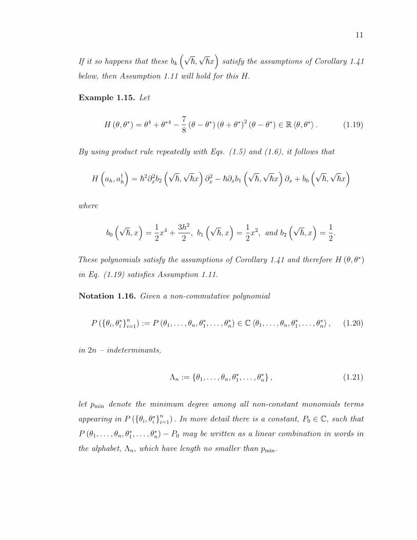
Example 1.15. Let

H (θ, θ∗) = θ4 + θ∗4 − 7

8(θ − θ∗) (θ + θ∗)2 (θ − θ∗) ∈ R 〈θ, θ∗〉 . (1.19)

By using product rule repeatedly with Eqs. (1.5) and (1.6), it follows that

H(ah, a

†h

)= ~2∂2

xb2

(√~,√~x)∂2x − ~∂xb1

(√~,√~x)∂x + b0

(√~,√~x)

where

b0

(√~, x)

=1

2x4 +

3h2

2, b1

(√~, x)

=1

2x2, and b2

(√~, x)

=1

2.

These polynomials satisfy the assumptions of Corollary 1.41 and therefore H (θ, θ∗)

in Eq. (1.19) satisfies Assumption 1.11.

Notation 1.16. Given a non-commutative polynomial

P (θi, θ∗i ni=1) := P (θ1, . . . , θn, θ

∗1, . . . , θ

∗n) ∈ C 〈θ1, . . . , θn, θ

∗1, . . . , θ

∗n〉 , (1.20)

in 2n – indeterminants,

Λn := θ1, . . . , θn, θ∗1, . . . , θ

∗n , (1.21)

let pmin denote the minimum degree among all non-constant monomials terms

appearing in P (θi, θ∗i ni=1) . In more detail there is a constant, P0 ∈ C, such that

P (θ1, . . . , θn, θ∗1, . . . , θ

∗n)− P0 may be written as a linear combination in words in

the alphabet, Λn, which have length no smaller than pmin.

12

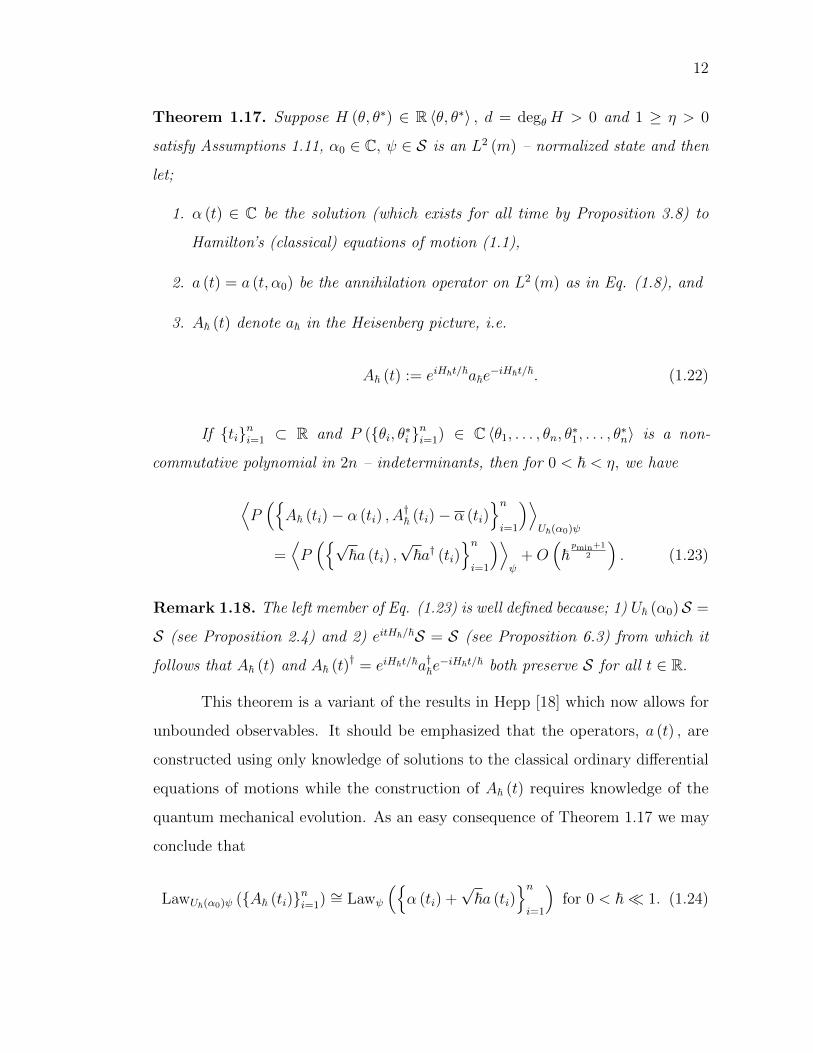
Theorem 1.17. Suppose H (θ, θ∗) ∈ R 〈θ, θ∗〉 , d = degθH > 0 and 1 ≥ η > 0

satisfy Assumptions 1.11, α0 ∈ C, ψ ∈ S is an L2 (m) – normalized state and then

let;

1. α (t) ∈ C be the solution (which exists for all time by Proposition 3.8) to

Hamilton’s (classical) equations of motion (1.1),

2. a (t) = a (t, α0) be the annihilation operator on L2 (m) as in Eq. (1.8), and

3. A~ (t) denote a~ in the Heisenberg picture, i.e.

A~ (t) := eiH~t/~a~e−iH~t/~. (1.22)

If tini=1 ⊂ R and P (θi, θ∗i ni=1) ∈ C 〈θ1, . . . , θn, θ

∗1, . . . , θ

∗n〉 is a non-

commutative polynomial in 2n – indeterminants, then for 0 < ~ < η, we have

⟨P(A~ (ti)− α (ti) , A

†~ (ti)− α (ti)

ni=1

)⟩U~(α0)ψ

=⟨P(√

~a (ti) ,√~a† (ti)

ni=1

)⟩ψ

+O(~pmin+1

2

). (1.23)

Remark 1.18. The left member of Eq. (1.23) is well defined because; 1) U~ (α0)S =

S (see Proposition 2.4) and 2) eitH~/~S = S (see Proposition 6.3) from which it

follows that A~ (t) and A~ (t)† = eiH~t/~a†~e−iH~t/~ both preserve S for all t ∈ R.

This theorem is a variant of the results in Hepp [18] which now allows for

unbounded observables. It should be emphasized that the operators, a (t) , are

constructed using only knowledge of solutions to the classical ordinary differential

equations of motions while the construction of A~ (t) requires knowledge of the

quantum mechanical evolution. As an easy consequence of Theorem 1.17 we may

conclude that

LawU~(α0)ψ (A~ (ti)ni=1) ∼= Lawψ

(α (ti) +

√~a (ti)

ni=1

)for 0 < ~ 1. (1.24)

13

The precise meaning of Eq. (1.24) is given in the following corollary.

Corollary 1.19. If we assume the same conditions and notations as in Theorem

1.17, then (for 0 < ~ < η)

⟨P(A~ (ti) , A

†~ (ti)

ni=1

)⟩U~(α0)ψ

=⟨P(α (ti) +

√~a (ti) , α (ti) +

√~a† (ti)

ni=1

)⟩ψ

+O (~) . (1.25)

By expanding out the right side of Eq.(1.25), it follows that

⟨P(A~ (ti) , A

†~ (ti)

ni=1

)⟩U~(α0)ψ

= P (α (ti) , α (ti)ni=1) +√~⟨P1

(α (ti) : a (ti) , a

† (ti)ni=1

)⟩ψ

+O (~)

(1.26)

where P1 (α (ti) : θi, θ∗i ni=1) is a degree one homogeneous polynomial of θi, θ∗i

ni=1

with coefficients depending smoothly on α (ti)ni=1 . Equation (1.26) states that

the quantum expectation values,

⟨P(A~ (ti) , A

†~ (ti)

ni=1

)⟩U~(α0)ψ

, (1.27)

closely track the corresponding classical values P (α (ti) , α (ti)ni=1) . The√~ term

in Eq. (1.26) represent the first quantum corrections (or fluctuations ) beyond the

leading order classical behavior.

Remark 1.20. If both H (θ, θ∗) , H (θ, θ∗) ∈ R 〈θ, θ∗〉 both satisfy Assumption 1.11

and are such that Hcl (α) := H (α, α) and Hcl (α) := H (α, α) are equal modulo a

constant, then Eq. (1.26) also holds with the A~ (ti) and A†~ (ti) appearing on the

left side of this equation being replaced by

eiH~ti/~a~e−iH~ti/~ and eiH~ti/~a†~e

−iH~ti/~

14

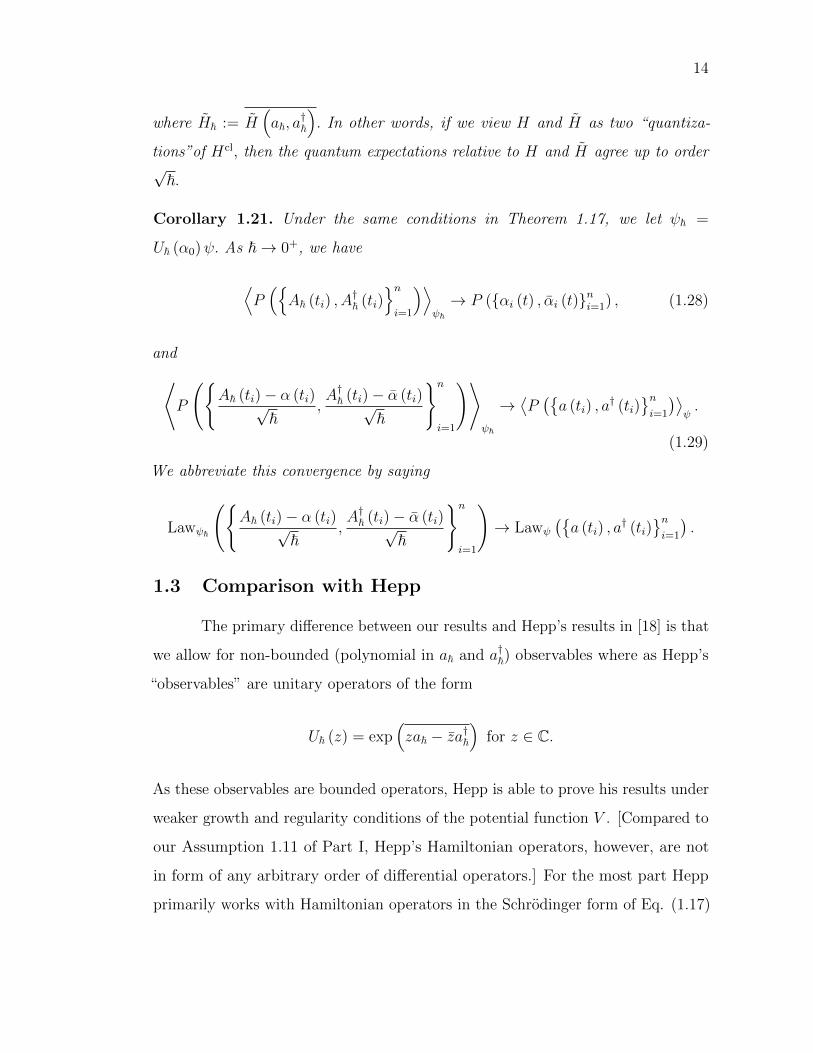
where H~ := H(a~, a

†~

). In other words, if we view H and H as two “quantiza-

tions”of Hcl, then the quantum expectations relative to H and H agree up to order√~.

Corollary 1.21. Under the same conditions in Theorem 1.17, we let ψ~ =

U~ (α0)ψ. As ~→ 0+, we have

⟨P(A~ (ti) , A

†~ (ti)

ni=1

)⟩ψ~→ P (αi (t) , αi (t)ni=1) , (1.28)

and⟨P

(A~ (ti)− α (ti)√

~,A†~ (ti)− α (ti)√

~

n

i=1

)⟩ψ~

→⟨P(a (ti) , a

† (ti)ni=1

)⟩ψ.

(1.29)

We abbreviate this convergence by saying

Lawψ~

(A~ (ti)− α (ti)√

~,A†~ (ti)− α (ti)√

~

n

i=1

)→ Lawψ

(a (ti) , a

† (ti)ni=1

).

1.3 Comparison with Hepp

The primary difference between our results and Hepp’s results in [18] is that

we allow for non-bounded (polynomial in a~ and a†~) observables where as Hepp’s

“observables” are unitary operators of the form

U~ (z) = exp(za~ − za†~

)for z ∈ C.

As these observables are bounded operators, Hepp is able to prove his results under

weaker growth and regularity conditions of the potential function V . [Compared to

our Assumption 1.11 of Part I, Hepp’s Hamiltonian operators, however, are not

in form of any arbitrary order of differential operators.] For the most part Hepp

primarily works with Hamiltonian operators in the Schrodinger form of Eq. (1.17)

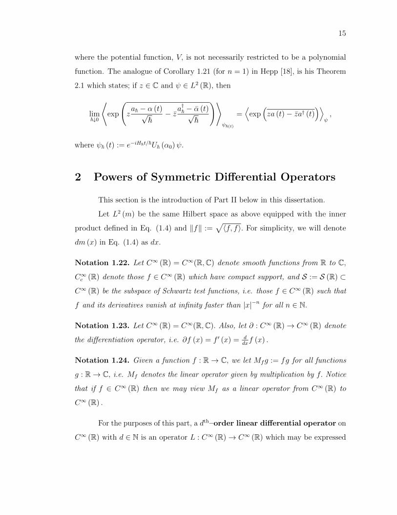
15

where the potential function, V, is not necessarily restricted to be a polynomial

function. The analogue of Corollary 1.21 (for n = 1) in Hepp [18], is his Theorem

2.1 which states; if z ∈ C and ψ ∈ L2 (R), then

lim~↓0

⟨exp

(za~ − α (t)√

~− z a

†~ − α (t)√

~

)⟩ψ~(t)

=⟨

exp(za (t)− za† (t)

)⟩ψ,

where ψ~ (t) := e−iH~t/~U~ (α0)ψ.

2 Powers of Symmetric Differential Operators

This section is the introduction of Part II below in this dissertation.

Let L2 (m) be the same Hilbert space as above equipped with the inner

product defined in Eq. (1.4) and ‖f‖ :=√〈f, f〉. For simplicity, we will denote

dm (x) in Eq. (1.4) as dx.

Notation 1.22. Let C∞ (R) = C∞(R,C) denote smooth functions from R to C,

C∞c (R) denote those f ∈ C∞ (R) which have compact support, and S := S (R) ⊂

C∞ (R) be the subspace of Schwartz test functions, i.e. those f ∈ C∞ (R) such that

f and its derivatives vanish at infinity faster than |x|−n for all n ∈ N.

Notation 1.23. Let C∞ (R) = C∞(R,C). Also, let ∂ : C∞ (R)→ C∞ (R) denote

the differentiation operator, i.e. ∂f (x) = f ′ (x) = ddxf (x) .

Notation 1.24. Given a function f : R→ C, we let Mfg := fg for all functions

g : R→ C, i.e. Mf denotes the linear operator given by multiplication by f. Notice

that if f ∈ C∞ (R) then we may view Mf as a linear operator from C∞ (R) to

C∞ (R) .

For the purposes of this part, a dth–order linear differential operator on

C∞ (R) with d ∈ N is an operator L : C∞ (R)→ C∞ (R) which may be expressed

16

as

L =d∑

k=0

Mak∂k =

d∑k=0

ak∂k (1.30)

for some akdk=0 ⊂ C∞ (R,C) . The symbol of L, σ = σL, is the function on R×R

defined by

σL (x, ξ) :=d∑

k=0

ak (x) (iξ)k . (1.31)

Remark 1.25. The action of L on C∞c (R) completely determines the coefficients,

akdk=0 . Indeed, suppose that x0 ∈ R and 0 ≤ k ≤ d and let ϕ (x) := (x− x0)k χ (x)

where χ ∈ C∞c (R) such that χ= 1 in a neighborhood of x0. Then an elementary

computation shows k! · ak (x0) = (Lϕ) (x0) . In particular if Lϕ ≡ 0 for all ϕ ∈

C∞c (R) then ak ≡ 0 for 0 ≤ k ≤ d and hence Lϕ ≡ 0 for all ϕ ∈ C∞ (R) .

Definition 1.26 (Formal adjoint and symmetry). Suppose L is a linear differential

operator on C∞ (R) as in Eq. (1.30). Then L†

: C∞ (R) → C∞ (R) denote the

formal adjoint of L given by the differential operator,

L† =d∑

k=0

(−1)k ∂kMak on C∞ (R) . (1.32)

Moreover L is said to be symmetric if L† = L on C∞ (R) .

Remark 1.27. Using Remark 1.25, one easily shows L† may alternatively be

characterized as that unique dth–order differential operator on C∞ (R) such that

〈Lf, g〉 =⟨f, L†g

⟩for all f, g ∈ C∞c (R) . (1.33)

From this characterization it is then easily verified that;

1. The dagger operation is an involution, in particular L†† = L and if S is

another linear differential operator on C∞ (R) , then (LS)† = S†L†.

17

2. L is symmetric iff 〈Lf, g〉 = 〈f, Lg〉 for all f, g ∈ C∞c (R) .

Proposition 10.2 below shows if akdk=0 ⊂ C∞ (R,R) , then L = L† iff

d = 2m is even and there exists blml=0 ⊂ C∞ (R,R) such that

L = L (blml=0) :=m∑l=0

(−1)l∂lbl(x)∂l. (1.34)

The factor of (−1)l is added for later convenience. The coefficients blml=0 are

uniquely determined by a2lml=0 (the even coefficients in Eq. (1.30) and in turn the

coefficients ak2mk=0 are determined by the blml=0 , see Lemma 10.4 and Theorem

10.7 respectively. We say that L is written in divergence form when L is expressed

as in Eq. (1.34).

From now on let us assume that akdk=0 ⊂ C∞ (R,R) and L is given as in

Eq. (1.30). For each n ∈ N, Ln is a dn order differential operator on C∞ (R) and

hence there exists Ak2mnk=0 ⊂ C∞ (R,C) such that

Ln =dn∑k=0

Ak∂k. (1.35)

If we further assume that L is symmetric (so d = 2m for some m ∈ N0), then by

Remark 1.27 Ln is a symmetric 2mn - order differential operator. Therefore by

Proposition 10.2, there exists B`mn`=0 ⊂ C∞ (R,R) so that Ln may be written in

divergence form as

Ln =mn∑`=0

(−1)` ∂`B`∂`. (1.36)

Information about the coefficients Ak2mnk=0 and B`mn`=0 in terms of the divergence

form coefficients blml=0 of L may be found in Propositions 11.7 and Proposition

11.8 respectively.

Let R [x] be the space of polynomial functions in one variable, x, with real

coefficients.

18

Remark 1.28. If the coefficients, akd=2mk=0 , of L in the Eq. (1.30) are in R [x] ,

then L and L† are both linear differential operator on C∞ (R) which leave S invariant.

Moreover by simple integration by parts Eq. (1.33) holds with C∞c (R) replaced by

S, i.e. 〈Lf, g〉 =⟨f, L†g

⟩for all f, g ∈ S.

Notation 1.29. For the remainder of this introduction we are going to assume

L is symmetric (L = L†), L is given in divergence form as in Eq. (1.34) with

blml=0 ⊂ R [x] , and we now view L as an operator on L2 (R,m) with D (L) = S ⊂

L2 (m) . In other words, we are going to replace L by L|S .

The main results of Part II will now be summarized in the next two sections.

2.1 Essential self-adjointness results

Theorem 1.30. Let m ∈ N, blml=0 ⊂ R [x] with bm (x) 6= 0 and assume;

1. either infx bl (x) > 0 or bl ≡ 0 and

2. deg (bl) ≤ max deg (b0) , 0 whenever 1 ≤ l ≤ m. [The zero polynomial is

defined to be of degree −∞.]

If L is the unbounded operator on L2 (m) as in Notation 1.29, then Ln (for

which D (Ln) is still S) is essentially self-adjoint for all n ∈ N.

Remark 1.31. Notice that assumption 1 of Theorem 1.30 implies deg (bl) is even

and the leading order coefficient of bl is positive unless bl ≡ 0.

Let us recall [Subspace Symmetry] in Definition 1.9 Let S be a dense

subspace of a Hilbert space K and A be a linear operator on K. Then A is said to

be symmetric on S if S ⊆ D (A) and

〈Aψ,ψ〉K = 〈ψ,Aψ〉K for all ψ ∈ S.

The equality is equivalent to say A|S ⊆ (A|S)∗ or A ⊆ A∗ if D (A) = S.

19

Remark 1.32. Using Remark 1.27, it is easy to see that L with polynomial coeffi-

cients is symmetric on C∞ (R) as in Definition 1.26 if and only if L is symmetric

on S as in Definition 1.9.

Therefore, there are three different partial ordering S, and ≤ (see

Notation 1.10) on symmetric operators on a Hilbert space.

There is a sizable literature dealing with similar essential self-adjointness in

Theorem 1.30, see for example [3,21,31]. Suppose that b2, b1, and b0 are smooth

real-valued functions of x ∈ R and T is a differential operator on C∞c (R) ⊆ L2 (m)

defined by,

T = −∂b2 (x) ∂ + b0 (x) + i (b1 (x) ∂ + ∂b1 (x)) .

Kato [21] shows T n is essentially self-adjoint for all n ∈ N when b2 = 1, b1 = 0

and −a − b |x|2 C∞c (R) T for some constants a and b. Chernoff [3] gives the

same conclusion under certain assumptions on b2 and T. For example, Chernoff’s

assumptions would hold if b2, b1 and b0 are real valued polynomial functions such

that deg (b2) ≤ 2 and b2 is positive and T is semi-bounded on C∞c (R) . In contrast,

Theorem 1.30 allows for higher order differential operators but does not allow for

non-polynomial coefficients. [However, the methods in Part II can be pushed further

in order to allow for certain non-polynomial coefficients.]

There are also a number of results regarding essential self-adjointness in

the pseudo-differential operator literature, the reader may be referred to, for

example, [6, 26, 27, 36, 39, 42]. In fact, our proof of Theorem 1.30 will be an

adaptation of an approach found in Theorem 3.1 in [26].

2.2 Operator Comparison Theorems

Motivated by ~ scaled quantization we picked in Definition 1.3 and the

important paper by [18], we will define a scaled version of L (see Notation 1.33)

20

where for any ~ > 0 we make the following replacements in Eq. (1.34),

x→√~Mx and ∂ →

√~∂. (1.37)

For reasons explained in Theorem B.2 of the appendix, we are lead to consider a

more general class of operators parametrized by ~ > 0.

Notation 1.33. Let

bl,~ (·) : 0 ≤ l ≤ m and ~ > 0 ⊂ R [x] , (1.38)

and then define

L~ = L(

~lbl,~(√~ (·))

ml=0

)=

m∑l=0

(−~)l∂lbl,~(√~ (·))∂l on S. (1.39)

We now record an assumption which is needed in a number of the results

stated below.

Assumption 1.34. Let m ∈ N0. We say bl,~ml=0 ⊂ R [x] and η > 0 satisfies

Assumption 1.34 if the following conditions hold.

1. For 0 ≤ l ≤ m, bl,~(x) =∑2ml

j=0 αl,j (~)xj is a real polynomial of x where αl,j

is a real continuous function on [0, η] .

2. For all 0 < ~ < η,

2ml = deg(bl,~) ≤ deg(bl−1,~) = 2ml−1 for 1 ≤ l ≤ m. (1.40)

21

3. We have,

cbm := infx∈R,0<~<η

bm,~(x) > 0 and (1.41)

cα := min0≤l≤m

inf0<~<η

αl,2ml (~) > 0, (1.42)

i.e. bm,~(x) is positive uniformly in x ∈ R and 0 < ~ < η and leading orders,

αl,2ml (~) , of all bl,~ ∈ R [x] are uniformly strictly positive.

Remark 1.35. Conditions (1) and (3) of Assumption 1.34 implies there exists

A ∈ (0,∞) so that

min0≤l≤m

inf0<~<η

inf|x|≥A

bl,~(x) > 0.

Furthermore, if k ≥ 1, 0 ≤ l1, . . . , lk ≤ m, and q~ (x) = bl1,~ (x) . . . blk,~ (x) ∈ R [x] ,

then

q~ (x) =2M∑i=0

Qi (~) · xi

where M = ml1 + . . . + mlk , each of the coefficients, Qi (~) is uniformly bounded

for 0 < ~ < η, and

inf0<~<η

Q2M (~) = inf0<~<η

αl1,ml1 ...αlk,mlk (~) ≥ ckα > 0.

From these remarks one easily shows inf0<~<η infx∈R q~ (x) > −∞.

The second main goal of Part II is to find criteria on two symmetric dif-

ferential operators L~ and L~ so that for each n ∈ N, there exists Kn < ∞ such

that

Ln~ S Kn

(Ln~ + I

). (1.43)

(As usual I denotes the identity operator here and S is as in Notation 1.10.) For

some perspective let us recall the Lowner-Heinz inequality.

22

Theorem 1.36 (Lowner-Heinz inequality). If A and B are two non-negative self-

adjoint operators on a Hilbert space, K, such that A ≤ B, then Ar ≤ Br for

0 ≤ r ≤ 1.

Lowner proved this result for finite dimensional matrices in [25] and Heinz

extended it to bounded operators in a Hilbert space in [16]. Later, both Heinz

in [16] and Kato in Theorem 2 of [19] extended the result for unbounded operators,

also see Proposition 10.14 of [35]. There is a large literature on so called “operator

monotone functions,” e.g. [2, 7], Theorem 18 of [29], [30] and [38]. It is well known

(see Section 10.3 of [35] for more background) that f (x) = xr is not an operator

monotone for r > 1, see [35, Example 10.3] for example. This indicates that proving

operator inequalities of the form in Eq. (1.43) is somewhat delicate. Our main

result in this direction is the subject of the next theorem.

Theorem 1.37 (Operator Comparison Theorem). Suppose that L~ and L~ are two

linear differential operators on S given by

L~ =

mL∑l=0

(−~)l∂lbl,~(√~x)∂l and L~ =

mL∑l=0

(−~)l∂lbl,~(√~x)∂l,

with polynomial coefficients,bl,~(x)

mLl=0

and bl,~(x)mLl=0 satisfying Assumption

1.34 with constants ηL and ηL respectively. Let η = minηL, ηL. If we further

assume that mL ≤ mL and there exists c1 and c2 such that

∣∣∣bl,~ (x)∣∣∣ ≤ c1 (bl,~ (x) + c2) ∀ 0 ≤ l ≤ mL and 0 < ~ < η, (1.44)

then for any n ∈ N there exists C1 and C2 such that

Ln~ S C1 (Ln~ + C2) for all 0 < ~ < η. (1.45)

Corollary 1.38. If bl,~(x)mLl=0 and η > 0 satisfy Assumption 1.34, then there

23

exists C ∈ R such that CI S L~ for all 0 < ~ < η.

Proof. Define L~ = I, i.e. we are taking mL = 0 and b0,~ (x) = 1. It then

follows from Theorem 1.37 with n = 1 that there exists C1, C2 ∈ (0, ∞) such that

I = L~ S C1L~ + C1C2 and hence L~ + C2 S C−11 I.

A similar result to Theorem 1.37 may be found in the Theorem 1.1 of [38].

The paper [38] compares the standard Laplacian −4 with an operator of H0 in

the form of −∑d

i,j ∂icij (x) ∂j with coefficients cijdi,j=1 lying in a Sobolev spaces

Wm+1,∞ (Rd)

for some m ∈ N and D (H0) = W∞,2 (Rd). The theorem shows that

if H0 is a symmetric, positive and subelliptic of order γ ∈ (0, 1] then H0 is positive

self-adjoint and for all α ∈[0, m+1+γ−1

2

], there exists Cα such that

(−∆)2αγ ≤ Cα(I +H0

)2α.

Theorem 1.37 also has a similar flavor to results in Nelson [28]. However, we have

not seen how to use Nelson’s result in our context.

As a corollary of Theorem 1.30 and aspects of the proof of Theorem 1.37

given in Chapter 14 below, we have the following corollaries which are proved in

Section 3 in Chapter 14 below.

Corollary 1.39. Supposed bl,~ (x)ml=0 ⊂ R [x] and η > 0 satisfies Assumption

1.34, L~ is the operator in the Eq. (1.39), and suppose that C ≥ 0 has been chosen

so that 0 S L~ + CI for all 0 < ~ < η. (The existence of C is guaranteed by

Corollary 1.38.) Then for any 0 < ~ < η, L~ + CI is a non-negative self-adjoint

operator on L2 (m) and S is a core for(L~ + C

)rfor all r ≥ 0.

Corollary 1.40. Suppose that L~ and L~ are two linear differential operators and

η > 0 as in Theorem 1.37. If C ≥ 0 and C ≥ 0 are chosen so that L~ + C S I

and L~ + C S 0 (as is possible by Corollary 1.38), then L~ + C and L~ + C are

24

non-negative self adjoint operators and for each r ≥ 0 there exists Cr such that

(L~ + C

)r Cr

(L~ + C

)r ∀ 0 < ~ < η. (1.46)

From Definitions 1.3 and 1.4 and Corollary 3.17, the positive self-adjoint

number operator, N , on L2 (m) is defined as the closure of

−1

2∂2 +

1

2x2 − 1

2on S. (1.47)

The next corollary is a direct consequence from Corollaries 1.39 and 1.40

where L~ = N~ in Eq. (1.46).

Corollary 1.41. Suppose m ≥ 1, bl,~(·)ml=0 ⊂ R [x] and η > 0 satisfy Assumption

1.34, and L~ is the operator on S defined in Eq. (1.39). If C ≥ 0 is chosen so that

I S L~ + C (see Corollary 1.38), then;

1. L~ + C is a non-negative self-adjoint operator on L2 (m) for all 0 < ~ < η.

2. S is a core for(L~ + C

)rfor all r ≥ 0 and 0 < ~ < η.

3. If we further supposed deg(b0,~) ≥ 2, then there exists Cr > 0 such that

N r~ Cr

(L~ + C

)r(1.48)

for all 0 < ~ < η and r ≥ 0.1

1By the spectral theorem one shows D(∣∣L~

∣∣r) = D((L~ + C

)r).

Part I

On the classical limit of quantum

mechanics

25

Chapter 2

Background and Setup

In this chapter we will expand on the basic setup described above and recall

some basic facts that will be needed throughout Part I

1 Classical Setup

In Part I, we take configuration space to be R so that our classical state space

is T ∗R ∼= R2. [Extensions to higher and to infinite dimensions will be considered

elsewhere.] Following Hepp [18], we identify T ∗R with C via

T ∗R 3 (ξ, π)→ α :=1√2

(ξ + iπ) . (2.1)

Taking in account the “√

2”above, we set

∂

∂α:=

1√2

(∂ξ − i∂π) and∂

∂α:=

1√2

(∂ξ + i∂π)

so that ∂∂αα = 1 = ∂

∂αα and ∂

∂αα = 0 = ∂

∂αα. As usual given a smooth real valued

function,1 Hcl (ξ, π) , on T ∗R we say (ξ (t) , π (t)) solves Hamilton’s equations of

1Later Hcl will be the symbol of a symmetric element of H ∈ C 〈θ, θ∗〉 as described in section4.

26

27

motion provided,

ξ (t) = Hclπ (ξ (t) , π (t)) and π (t) = −Hcl

ξ (ξ (t) , π (t)) (2.2)

where Hclπ := ∂Hcl/∂π and Hcl

ξ := ∂Hcl/∂ξ . A simple verifications shows; if

α (t) :=1√2

(ξ (t) + iπ (t)) ,

then (ξ (t) , π (t)) solves Hamilton’s Eqs. (2.2) iff α (t) satisfies

iα (t) =

(∂

∂αHcl

)(α (t)) (2.3)

where

Hcl (α) := Hcl (ξ, π) where α =1√2

(ξ + iπ) ∈ C.

In the future we will identify Hcl with Hcl and drop the tilde from our notation.

Example 2.1. If H (α) = |α|2 + 12|α|4 , then the associated Hamiltonian equations

of motion are given by

iα =∂

∂α

(αα +

1

2α2α2

)= α + α2α = α + |α|2 α.

Proposition 2.2. Let z (t) := Φ′ (t, α0) z be the real differential of the flow asso-

ciated to Eq. (1.1) as in Eq. (1.2). Then z (t) satisfies z (0) = z and

iz (t) = u (t) z (t) + v (t) z (t) , (2.4)

where

u (t) :=

(∂2

∂α2Hcl

)(α (t)) ∈ C and v (t) =

(∂2

∂α∂αHcl

)(α (t)) ∈ R. (2.5)

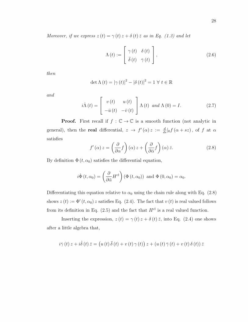
28

Moreover, if we express z (t) = γ (t) z + δ (t) z as in Eq. (1.3) and let

Λ (t) :=

γ (t) δ (t)

δ (t) γ (t)

, (2.6)

then

det Λ (t) = |γ (t)|2 − |δ (t)|2 = 1 ∀ t ∈ R

and

iΛ (t) =

v (t) u (t)

−u (t) −v (t)

Λ (t) and Λ (0) = I. (2.7)

Proof. First recall if f : C→ C is a smooth function (not analytic in

general), then the real differential, z → f ′ (α) z := dds|0f (α + sz) , of f at α

satisfies

f ′ (α) z =

(∂

∂αf

)(α) z +

(∂

∂αf

)(α) z. (2.8)

By definition Φ (t, α0) satisfies the differential equation,

iΦ (t, α0) =

(∂

∂αHcl

)(Φ (t, α0)) and Φ (0, α0) = α0.

Differentiating this equation relative to α0 using the chain rule along with Eq. (2.8)

shows z (t) := Φ′ (t, α0) z satisfies Eq. (2.4). The fact that v (t) is real valued follows

from its definition in Eq. (2.5) and the fact that Hcl is a real valued function.

Inserting the expression, z (t) = γ (t) z + δ (t) z, into Eq. (2.4) one shows

after a little algebra that,

iγ (t) z + iδ (t) z =(u (t) δ (t) + v (t) γ (t)

)z + (u (t) γ (t) + v (t) δ (t)) z

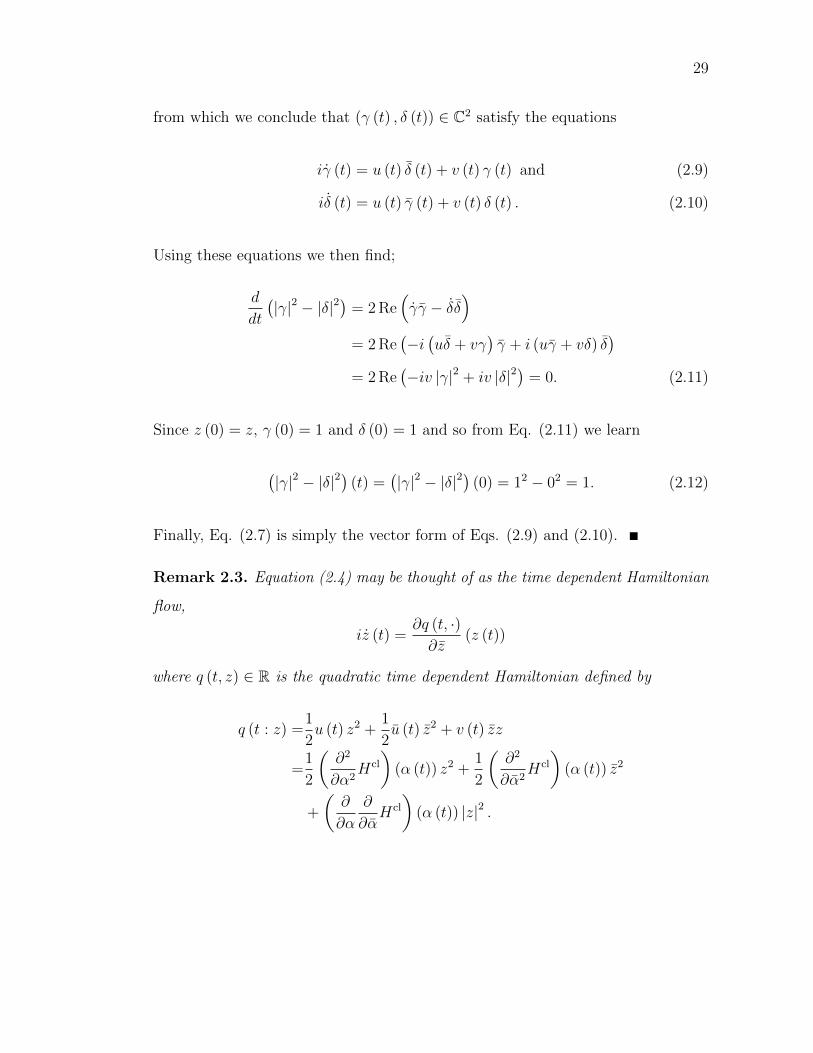
29

from which we conclude that (γ (t) , δ (t)) ∈ C2 satisfy the equations

iγ (t) = u (t) δ (t) + v (t) γ (t) and (2.9)

iδ (t) = u (t) γ (t) + v (t) δ (t) . (2.10)

Using these equations we then find;

d

dt

(|γ|2 − |δ|2

)= 2 Re

(γγ − δδ

)= 2 Re

(−i(uδ + vγ

)γ + i (uγ + vδ) δ

)= 2 Re

(−iv |γ|2 + iv |δ|2

)= 0. (2.11)

Since z (0) = z, γ (0) = 1 and δ (0) = 1 and so from Eq. (2.11) we learn

(|γ|2 − |δ|2

)(t) =

(|γ|2 − |δ|2

)(0) = 12 − 02 = 1. (2.12)

Finally, Eq. (2.7) is simply the vector form of Eqs. (2.9) and (2.10).

Remark 2.3. Equation (2.4) may be thought of as the time dependent Hamiltonian

flow,

iz (t) =∂q (t, ·)∂z

(z (t))

where q (t, z) ∈ R is the quadratic time dependent Hamiltonian defined by

q (t : z) =1

2u (t) z2 +

1

2u (t) z2 + v (t) zz

=1

2

(∂2

∂α2Hcl

)(α (t)) z2 +

1

2

(∂2

∂α2Hcl

)(α (t)) z2

+

(∂

∂α

∂

∂αHcl

)(α (t)) |z|2 .

30

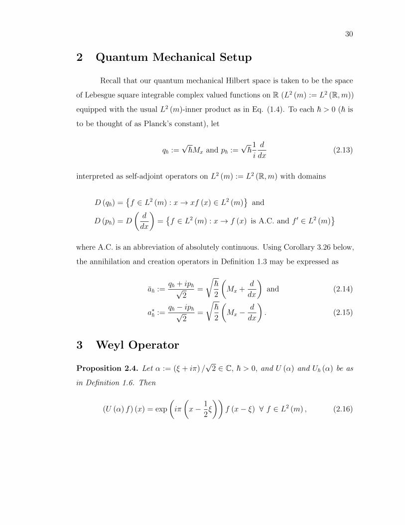
2 Quantum Mechanical Setup

Recall that our quantum mechanical Hilbert space is taken to be the space

of Lebesgue square integrable complex valued functions on R (L2 (m) := L2 (R,m))

equipped with the usual L2 (m)-inner product as in Eq. (1.4). To each ~ > 0 (~ is

to be thought of as Planck’s constant), let

q~ :=√~Mx and p~ :=

√~

1

i

d

dx(2.13)

interpreted as self-adjoint operators on L2 (m) := L2 (R,m) with domains

D (q~) =f ∈ L2 (m) : x→ xf (x) ∈ L2 (m)

and

D (p~) = D

(d

dx

)=f ∈ L2 (m) : x→ f (x) is A.C. and f ′ ∈ L2 (m)

where A.C. is an abbreviation of absolutely continuous. Using Corollary 3.26 below,

the annihilation and creation operators in Definition 1.3 may be expressed as

a~ :=q~ + ip~√

2=

√~2

(Mx +

d

dx

)and (2.14)

a∗~ :=q~ − ip~√

2=

√~2

(Mx −

d

dx

). (2.15)

3 Weyl Operator

Proposition 2.4. Let α := (ξ + iπ) /√

2 ∈ C, ~ > 0, and U (α) and U~ (α) be as

in Definition 1.6. Then

(U (α) f) (x) = exp

(iπ

(x− 1

2ξ

))f (x− ξ) ∀ f ∈ L2 (m) , (2.16)

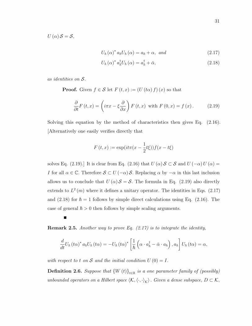
31

U (α)S = S,

U~ (α)∗ a~U~ (α) = a~ + α, and (2.17)

U~ (α)∗ a†~U~ (α) = a†~ + α, (2.18)

as identities on S.

Proof. Given f ∈ S let F (t, x) := (U (tα) f) (x) so that

∂

∂tF (t, x) =

(iπx− ξ ∂

∂x

)F (t, x) with F (0, x) = f (x) . (2.19)

Solving this equation by the method of characteristics then gives Eq. (2.16).

[Alternatively one easily verifies directly that

F (t, x) := exp(itπ(x− 1

2tξ))f(x− tξ)

solves Eq. (2.19).] It is clear from Eq. (2.16) that U (α)S ⊂ S and U (−α)U (α) =

I for all α ∈ C. Therefore S ⊂ U (−α)S. Replacing α by −α in this last inclusion

allows us to conclude that U (α)S = S. The formula in Eq. (2.19) also directly

extends to L2 (m) where it defines a unitary operator. The identities in Eqs. (2.17)

and (2.18) for ~ = 1 follows by simple direct calculations using Eq. (2.16). The

case of general ~ > 0 then follows by simple scaling arguments.

Remark 2.5. Another way to prove Eq. (2.17) is to integrate the identity,

d

dtU~ (tα)∗ a~U~ (tα) = −U~ (tα)∗

[1

~

(α · a†~ − α · a~

), a~

]U~ (tα) = α,

with respect to t on S and the initial condition U (0) = I.

Definition 2.6. Suppose that W (t)t∈R is a one parameter family of (possibly)

unbounded operators on a Hilbert space 〈K, 〈·, ·〉K〉 . Given a dense subspace, D ⊂ K,

32

we say W (t) is strongly ‖·‖K-norm differentiable on D if 1) D ⊂ D (W (t))

for all t ∈ R and 2) for all ψ ∈ D, t → W (t)ψ is ‖·‖K-norm differentiable. For

notational simplicity we will write W (t)ψ for ddt

[W (t)ψ] .

Proposition 2.7. If R 3 t → α (t) ∈ C is a C1 function and N := N~|~=1 the

number operator defined in Eq. (1.11), then U (α (t))t∈R is strongly L2 (m)-norm

differentiable on D(√N)

as in the Definition 2.6 and for all f ∈ D(√N)

we

have

d

dt(U (α (t)) f) =

(α (t) a∗ − α (t)a+ i Im

(α (t) α (t)

))U (α (t)) f

= U (α (t))(α (t) a∗ − α (t)a− i Im

(α (t) α (t)

))f.

Moreover, U (α (t)) preserves D(√N)

, Cc(R), and S.

Proof. From Corollary 3.26 below we know D(∂x) ∩D(Mx) = D(√N).

Using this fact, the proposition is a straightforward verification based on Eq. (2.16).

The reader not wishing to carry out these computations may find it instructive to

give a formal proof based on the algebraic fact that eA+B = eAeBe−12

[A,B] where A

and B are operators such that the commutator, [A,B] := AB − BA, commutes

with both A and B.

As we do not wish to make any particular choice of quantization scheme, in

Part I we will describe all operators as a non-commutative polynomial functions of

a~ and a†~. This is the topic of the next chapter.

4 Non-commutative Polynomial Expansions

Notation 2.8. Let C 〈θ, θ∗〉 be the space of non-commutative polynomials in the

non-commutative indeterminates. That is to say C 〈θ, θ∗〉 is the vector space over

33

C whose basis consists of words in the two letter alphabet, Λ1 = θ, θ∗ , cf. Eq.

(1.21). The general element, P (θ, θ∗) , of C 〈θ, θ∗〉 may be written as

P (θ, θ∗) =d∑

k=0

∑b=(b1,...,bk)∈Λk1

ck (b) b1 . . . bk, (2.20)

where d ∈ N0 and

ck (b) : 0 ≤ k ≤ d and b = (b1, . . . , bk)∈Λk

1

⊂ C.

If cd : Λd1 → C is not the zero function, we say d =: degθ P is the degree of P.

It is sometimes convenient to decompose P (θ, θ∗) in Eq. (2.20) as

P (θ, θ∗) =d∑

k=0

Pk (θ, θ∗) (2.21)

where

Pk (θ, θ∗) =∑

b1,...,bk∈Λ1

ck (b1, . . . , bk) b1 . . . bk. (2.22)

Polynomials of the form in Eq. (2.22) are said to be homogeneous of degree k.

By convention, P0 := P0 (θ, θ∗) is just an element of C. We endow C 〈θ, θ∗〉 with its

`1 – norm, |·| , defined for P as in Eq. (2.20) by

|P | :=d∑

k=0

|Pk| where |Pk| =∑

b=(b1,...,bk)∈Λk1

|ck (b)| . (2.23)

Definition 2.9 (Monomials). For b = (b1, . . . , bk) ∈ θ, θ∗k let ub ∈ C 〈θ, θ∗〉 be

the monomial,

ub (θ, θ∗) = b1 . . . bk (2.24)

with the convention that for k = 0 we associate the unit element u0 = 1.

34

As usual, we make C 〈θ, θ∗〉 into a non-commutative algebra with its natural

multiplication determined on the word basis elements ∪∞k=0

ub : b ∈θ, θ∗k

by

concatenation of words, i.e. ubud = u(b,d) where if d = (d1, . . . , dl) ∈ θ, θ∗l

(b,d) := (b1, . . . , bk, d1, . . . , dl) ∈ θ, θ∗k+l .

For example, θθθ∗ ·θ∗θ = θθθ∗θ∗θ. We also define a natural involution on C 〈θ, θ∗〉

determined by (θ)∗ = θ∗, (θ∗)∗ = θ, z∗ = z for z ∈ C, and (α · β)∗ = β∗α∗ for

α, β ∈ C 〈θ, θ∗〉 . Formally, if b = (b1, . . . , bk) ∈ θ, θ∗k , then

u∗b = b∗kb∗k−1 . . . b

∗1 = ub∗ where b∗ :=

(b∗k, b

∗k−1, . . . , b

∗1

). (2.25)

In what follows we will often denote an P ∈ C 〈θ, θ∗〉 by P (θ, θ∗) .

Definition 2.10 (Symmetric Polynomials). We say P ∈ C 〈θ, θ∗〉 is symmetric

provided P = P ∗.

If A is any unital algebra equipped with an involution, ξ → ξ†, and ξ is any

fixed element of A, then there exists a unique algebra homomorphism

P (θ, θ∗) ∈ C 〈θ, θ∗〉 → P(ξ, ξ†

)∈ A

determined by substituting ξ for θ and ξ† for θ∗. Moreover, the homomorphism

preserves involutions, i.e.[P(ξ, ξ†

)]†= P ∗

(ξ, ξ†

). The two special cases of this

construction that we need here are contained in the following two definitions.

Definition 2.11 (Classical Symbols). The symbol (or classical residue) of P ∈

C 〈θ, θ∗〉 is the function P cl ∈ C [z, z] (= the commutative polynomials in z and

z with complex coefficients) defined by P cl (α) := P (α, α) where we view C as a

commutative algebra with an involution given by complex conjugation.

35

Definition 2.12 (Polynomial Operators). If P (θ, θ∗) ∈ C 〈θ, θ∗〉 is a non-commutative

polynomial and ~ > 0, then P(a~, a

†~

)is a differential operator on L2 (m) whose

domain is S. [Notice that P(a~, a

†~

)preserves S, i.e. P

(a~, a

†~

)S ⊂ S.] We further

let P~ := P(a~, a

†~

)be the closure of P

(a~, a

†~

). Any linear differential operator

of the form P(a~, a

†~

)for some P (θ, θ∗) ∈ C 〈θ, θ∗〉 will be called a polynomial

operator.

We introduce the following notation in order to write out P(a~, a

†~

)more

explicitly.

Notation 2.13. For any ~ > 0 let Ξ~ : θ, θ∗ →a~, a

†~

be define by

Ξ~ (b) =

a~ if b = θ

a†~ if b = θ∗. (2.26)

In the special case where ~ = 1 we will simply denote Ξ1 by Ξ.

With this notation if P ∈ C 〈θ, θ∗〉 is as in Eq. (2.20), then P(a~, a

†~

)may

be written as,

P(a~, a

†~

)=

d∑k=0

∑b=(b1,...,bk)∈Λk1

ck (b) Ξ~ (b1) . . .Ξ~ (bk) (2.27)

or as

P(a~, a

†~

)=

d∑k=0

∑b=(b1,...,bk)∈Λk1

~k/2ck (b)ub

(a, a†

)(2.28)

Definition 2.14 (Monomial Operators). Any linear differential operator of the

form ub

(a, a†

)= Ξ1 (b1) . . .Ξ1 (bk) for some b = (b1, . . . , bk) ∈ θ, θ∗k and k ∈ N0

will be called a monomial operator.

Remark 2.15. If H (θ, θ∗) ∈ C 〈θ, θ∗〉 is symmetric (i.e. H = H∗), then;

36

1. H(a~, a

†~

)is a symmetric operator on S (i.e.

[H(a~, a

†~

)]†= H

(a~, a

†~

))

for any ~ > 0 and

2. Hcl (z) := H (z, z) is a real valued function on C.

Indeed, [H(a~, a

†~

)]†= H∗

(a~, a

†~

)= H

(a~, a

†~

)and

Hcl (α) := H (α, α) = H∗ (α, α) = H (α, α) = Hcl (α) .

The main point of Part I is to show under Assumption 1.11 on H that classical

Hamiltonian dynamics associated to Hcl determine the limiting quantum mechanical

dynamics determined by H~ := H(a~, a

†~

).

We have analogous definitions and statements for the non-commutative

algebra, C 〈θ1, . . . , θn, θ∗1, . . . , θ

∗n〉 , of non-commuting polynomials in 2n – indeter-

minants, Λn = θ1, . . . , θn, θ∗1, . . . , θ

∗n , as in Eq. (1.21).

Notation 2.16. Let C [x] 〈θ, θ∗〉 and C [α, α] 〈θ, θ∗〉 denote the non-commutative

polynomials in θ, θ∗ with coefficients in the commutative polynomial rings, C [x]

and C [α, α] respectively. For P ∈ C [x] 〈θ, θ∗〉 or P ∈ C [α, α] 〈θ, θ∗〉 we will write

degθ P to indicate that we are computing the degree relative to θ, θ∗ and not

relative to x or α, α .

For any α ∈ C and P (θ, θ∗) ∈ C 〈θ, θ∗〉 with d = degθ P, let Pk (α : θ, θ∗)dk=0 ⊂

C [α, α] 〈θ, θ∗〉 denote the unique homogeneous polynomials in C 〈θ, θ∗〉 with coeffi-

cients which are polynomials in α and α such that degθ Pk (α : θ, θ∗) = k and

P (θ + α, θ∗ + α) =d∑

k=0

Pk (α : θ, θ∗) . (2.29)

37

Example 2.17. If

P (θ, θ∗) = θθ∗θ + θ∗θθ∗

then

P (θ + α, θ∗ + α) = (θ + α) (θ∗ + α) (θ + α) + (θ∗ + α) (θ + α) (θ∗ + α)

= P0 + P1 + P2 + P≥3

where

P0 (α, θ, θ∗) = α2α + α2α = P cl (α)

P1 (α, θ, θ∗) =(2 |α|2 + α2

)θ +

(2 |α|2 + α2

)θ∗

=∂P cl

∂α(α) θ +

∂P cl

∂α(α) θ∗

P2 (α, θ, θ∗) = αθ2 + αθ∗2 + (α + α) θ∗θ + (α + α) θθ∗

=1

2

(∂2P cl

∂α2(α) θ2 +

∂2P cl

∂α2(α) θ∗2

)+d

dt|t=0

d

ds|s=0P (sθ + α, tθ∗ + α)

P≥3 (α, θ, θ∗) = θθ∗θ + θ∗θθ∗.

This example is generalized in the following theorem.

Theorem 2.18. Let P (θ, θ∗) ∈ C 〈θ, θ∗〉 and α ∈ C, then

P0 (α : θ, θ∗) = P cl (α)

P1 (α : θ, θ∗) =

[∂P cl

∂α(α) θ +

∂P cl

∂α(α) θ∗

]and

P2 (α : θ, θ∗) =1

2

(∂2P cl

∂α2(α) θ2 +

∂2P cl

∂α2(α) θ∗2

)+d

dt|t=0

d

ds|s=0P (sθ + α, tθ∗ + α) . (2.30)

38

where

d

dt|t=0

d

ds|s=0P (sθ + α, tθ∗ + α) =

∂2P cl

∂α∂α(α) θ∗θ mod θ∗θ = θθ∗

for all α ∈ C. So we have

P (θ + α, θ∗ + α)

= P cl (α) +

[∂P cl

∂α(α) θ +

(∂

∂αP cl

)(α) θ∗

]+ P2 (α : θ, θ∗) + P≥3 (α : θ, θ∗)

(2.31)

where the remainder term, P≥3 is a sum of homogeneous terms of degree 3 or more.

Moreover if P = P ∗, then P ∗2 = P2 and P ∗≥3 = P≥3.

Proof. If p = degθ P, then

P (tθ + α, tθ∗ + α) =

p∑k=0

tkPk (α : θ, θ∗) ∀ t ∈ R,

and it follows (by Taylor’s theorem) that

Pk (α : θ, θ∗) =1

k!

(d

dt

)k|t=0P (tθ + α, tθ∗ + α) . (2.32)

From Eq. (2.32),

P0 (α : θ, θ∗) = P (α, α) = P cl (α) and

P1 (α : θ, θ∗) =d

dt|t=0P (tθ + α, tθ∗ + α)

=d

dt|t=0P (tθ + α, α) +

d

dt|t=0P (α, tθ∗ + α)

=∂P cl

∂α(α) θ +

∂P cl

∂α(α) θ∗.

39

Similarly from Eq. (2.32),

P2 (α : θ, θ∗) =1

2

(d

dt

)2

|t=0P (tθ + α, tθ∗ + α)

=1

2

(d

dt

)2

|t=0 [P (tθ + α, α) + P (α, tθ∗ + α)]

+d

dt|t=0

d

ds|s=0P (sθ + α, tθ∗ + α)

=1

2

(∂2P cl

∂α2(α) θ2 +

∂2P cl

∂α2(α) θ∗2

)+d

dt|t=0

d

ds|s=0P (sθ + α, tθ∗ + α) .

If P (θ, θ∗) ∈ C 〈θ, θ∗〉 is symmetric, then P (tθ + α, tθ∗ + α) ∈ C 〈θ, θ∗〉 is

symmetric and hence from Eq. (2.32) it follows that Pk (α : θ, θ∗) ∈ C 〈θ, θ∗〉 is still

symmetric and therefore so is the remainder term,

P≥3 (α : θ, θ∗) =

p∑k=3

Pk (α : θ, θ∗) .

Chapter 3

Polynomial Operators

1 Algebra of Polynomial Operators

Notation 3.1. For b = (b1, . . . , bk) ∈ θ, θ∗k , p (b) , q (b) , and ` (b) be the Z –

valued functions defined by

p (b) := # i : bi = θ , q (b) := # i : bi = θ∗ , and (3.1)

` (b) :=k∑i=1

(1bi=θ∗ − 1bi=θ) = q (b)− p (b) . (3.2)

Thus p (b) (q (b)) is the number of θ’s (θ∗’s) in b and ` (b) counts the excess

number of θ∗’s over θ’s in b.

Lemma 3.2 (Normal Ordering). If P (θ, θ∗) ∈ C 〈θ, θ∗〉 with d = degθ P, then

there exists R (~ : θ, θ∗) ∈ C [~] 〈θ, θ∗〉 (a non-commutative polynomial in θ, θ∗

with polynomial coefficients in ~) such that degθ R (~ : θ, θ∗) ≤ d− 2 and

P(a~, a

†~

)=

∑0≤k,l; k+l≤d

1

k! · l!

(∂k+lP cl

∂αk∂αl

)(0) a†k~ a

l~ + ~R

(~ : a~, a

†~

)∀ ~ > 0.

Proof. By linearity it suffices to consider the case here P (θ, θ∗) is a

40

41

homogeneous polynomial of degree d which may be written as

P (θ, θ∗) =∑

b∈θ,θ∗dc (b)ub (θ, θ∗) =

d∑p=0

∑b∈θ,θ∗d

1p(b)=pc (b)ub (θ, θ∗) . (3.3)

Since

P (α, α) =d∑p=0

∑b∈θ,θ∗d

1p(b)=pc (b)

αpαd−pit follows that

1

(d− p)! · p!

(∂dP cl

∂αd−p∂αp

)(0) =

∑b∈θ,θ∗d

1p(b)=pc (b) .

On the other hand, if b ∈ θ, θ∗d and p := p (b) , then making use of the CCRs

of Eq. (1.7) it is easy to show there exists Rb (~, θ, θ∗) ∈ C [~] 〈θ, θ∗〉 such that

degθ Rb (~, θ, θ∗) ≤ d− 2 such that

ub

(a~, a

†~

)= a

†(d−p)~ ap~ + ~Rb

(~, a~, a†~

). (3.4)

Replacing θ by a~ and θ∗ by a†~ in Eq. (3.3) and using Eq. (3.4) we find,

P(a~, a

†~

)=

d∑p=0

∑b∈θ,θ∗d

1p(b)=pc (b)ub

(a~, a

†~

)

=d∑p=0

∑b∈θ,θ∗d

1p(b)=pc (b)

a†(d−p)~ ap~ + ~∑

b∈θ,θ∗dc (b)Rb

(~, a~, a†~

)

=d∑p=0

1

(d− p)! · p!

(∂dP cl

∂αd−p∂αp

)(0) a

†(d−p)~ ap~ + ~R

(~, a~, a†~

)

where

R (~, θ, θ∗) =∑

b∈θ,θ∗dc (b)Rb (~, θ, θ∗) .

42

Corollary 3.3. If P (θ, θ∗) and Q (θ, θ∗) are non-commutative polynomials such

that P cl = Qcl, then there exists R (~ : θ, θ∗) ∈ C [~] 〈θ, θ∗〉 with degθ R (~ : θ, θ∗) ≤

degθ (P −Q) (θ, θ∗)− 2 such that

P(a~, a

†~

)= Q

(a~, a

†~

)+ ~R

(~, a~, a†~

).

Proof. Apply Lemma 3.2 to the non-commutative polynomial, P (θ, θ∗)−

Q (θ, θ∗) .

Proposition 3.4. For all H ∈ C 〈θ, θ∗〉 , there exists a polynomial, pH ∈ C [z, z]

such that

H2

(α : a, a†

)=

1

2

(∂2Hcl

∂α2

)(α) a2 +

1

2

(∂2Hcl

∂α2

)(α) a†2 +

(∂2Hcl

∂α∂α

)(α) a†a+ pH (α, α) I

for all α ∈ C where H2 (α : θ, θ∗) is defined in Eq. (2.29).

Proof. As we have seen the structure of H2 (α : θ, θ∗) implies there exists

ρ, γ, δ ∈ C [α, α] such that

2H2 (α : θ, θ∗) = ρ (α, α) θ2 + ρ (α, α)θ∗2 + γ (α, α) θ∗θ + δ (α, α) θθ∗.

From this equation we find,

2H2 (α : z, z) = ρ (α, α) z2 + ρ (α, α)z2 + [γ (α, α) + δ (α, α)] zz

while form Eq. (2.30) we may conclude that

2H2 (α : z, z) =

(∂2Hcl

∂α2

)(α) z2 +

(∂2Hcl

∂α2

)(α) z2 + 2

(∂2Hcl

∂α∂α

)(α) zz. (3.5)

43

Comparing these last two equations shows,

(∂2Hcl

∂α2

)(α) = ρ (α, α) ,

(∂2Hcl

∂α2

)(α) = ρ (α, α), and(

∂2Hcl

∂α∂α

)(α) =

1

2[γ (α, α) + δ (α, α)] .

Using these last identities and the canonical commutations relations we find,

2H2

(α : a, a†

)= ρ (α, α) a2 + ρ (α, α)a†2 + γ (α, α) a†a+ δ (α, α) aa†

= ρ (α, α) a2 + ρ (α, α)a†2 + [γ (α, α) + δ (α, α)] a†a+ δ (α, α) I

=

(∂2Hcl

∂α2

)(α) a2 +

(∂2Hcl

∂α2

)(α) a†2 + 2

(∂2Hcl

∂α∂α

)(α) a†a+ pH (α, α) I

with pH (α, α) = δ (α, α) .

Proposition 3.4 and the following simple commutator formulas,

[a†a, a

]= −a,

[a†2, a

]= −2a†,[

a†a, a†]

= a†, and[a2, a†

]= 2a,

immediately give the following corollary.

Corollary 3.5. If H ∈ C 〈θ, θ∗〉 and α ∈ C, then

[H2

(α : a, a†

), a]

= −(∂2Hcl

∂α∂α

)(α) a−

(∂2Hcl

∂α2

)(α) a†

[H2

(α : a, a†

), a†]

=

(∂2Hcl

∂α2

)(α) a+

(∂2Hcl

∂α∂α

)(α) a†.

44

2 Expectations and variances for translated states

The next result is a fairly easy consequence of Proposition 2.4 and the

expansion of non-commutative polynomials into their homogeneous components.

Corollary 3.6 (Concentrated states). Let P (θ, θ∗) ∈ C 〈θ, θ∗〉 , ψ ∈ S, ~ > 0, and

α ∈ C, then

⟨P(a~, a

†~

)⟩U~(α)ψ

= P (α, α) +O(√

~)

(3.6)

VarU~(α)ψ

(P(a~, a

†~

))= O

(√~), (3.7)

and

lim~↓0

⟨P

(a~ − α√

~,a†~ − α√

~

)⟩U~(α)ψ

=⟨P(a, a†

)⟩ψ

(3.8)

where 〈·〉U~(α)ψ is defined in Definition 1.7. [In fact, the equality in the last equation

holds before taking the limit as ~→ 0.]

Proof. From Proposition 2.4 and Eq. (2.29),

U~ (α)∗ P(a~, a

†~

)U~ (α) = P

(a~ + α, a†~ + α

)=

d∑k=0

Pk

(α : a~, a

†~

)(3.9)

and hence

⟨P(a~, a

†~

)⟩U~(α)ψ

=⟨U~ (α)∗ P

(a~, a

†~

)U~ (α)

⟩ψ

=⟨P(a~ + α, a†~ + α

)⟩ψ

=

⟨d∑

k=0

Pk

(α : a~, a

†~

)⟩ψ

= P0 (α) +d∑

k=1

~k/2⟨Pk(α : a, a†

)⟩ψ

from which Eq. (3.6) follows where P0 (α) is defined in Notation 2.8. Similarly,

45

making use of the fact that (P 2)0 (α) = (P 20 ) (α)

⟨P 2(a~, a

†~

)⟩U~(α)ψ

=(P 2

0

)(α) +

2d∑k=1

~k/2⟨(P 2)k

(α : a, a†

)⟩ψ

(3.10)

and hence

VarU~(α)ψ

(P(a~, a

†~

))=(P 2

0

)(α) +

2d∑k=1

~k/2⟨(P 2)k

(α : a, a†

)⟩ψ

−

[(P0 (α) +

d∑k=0

~k/2⟨Pk(α : a, a†

)⟩ψ

)]2

= O(√

~).

Lastly, using Eq. (3.9) one shows,

⟨P

(a~ − α√

~,a†~ − α√

~

)⟩U~(α)ψ

=

⟨P

(a~ + α− α√

~,a†~ + α− α√

~

)⟩ψ

=⟨P(a, a†

)⟩ψ

which certainly implies Eq. (3.8).

Remark 3.7. If ψ ∈ S and α ∈ C, Eqs. (3.6) and (3.7) should be interpreted

to say that for small ~ > 0, U~ (α)ψ is a state which is concentrated in phase

space near α. Consequently, these are good initial states for discussing the classical

(~→ 0) limit of quantum mechanics.

The next result shows that, under Assumption 1.11, the classical equations

of motions in Eq. (1.1) have global solutions which remain bounded in time.

Proposition 3.8. If C and C1 are the constants appearing in Eq. (1.14) of

Assumption 1.11, α0 ∈ C, and α (t) ∈ C is the maximal solution of Hamilton’s

ordinary differential equations (1.1), then α (t) is defined for all time t and moreover,

|α (t)|2 ≤ C1

(Hcl (α (0)) + C

), (3.11)

46

where Hcl (α) := H (α, α) .

Proof. Equation (1.14) with β = 1 implies

〈N~〉ψ ≤ C1 〈H~ + C〉ψ for all ψ ∈ S. (3.12)

Replacing ψ by U~ (α)ψ in Eq. (3.12) and then letting ~ ↓ 0 gives (with the aid of

Corollary 3.6) the estimate,

|α|2 ≤ C1

(Hcl (α) + C

)for all α ∈ C. (3.13)

If α (t) solves Hamilton’s Eq. (1.1) then Hcl (α (t)) = Hcl (α (0)) for all t. As the

level sets of Hcl are compact because of the estimate in Eq. (3.13) there is no

possibility for α (t) to explode and hence solutions will exist for all times t and

moreover must satisfy the estimate in Eq. (3.11).

3 Analysis of Monomial Operators of a and a†

In this section, recall that a = a1 and a† = a†1 as in Definition 1.3. Let

Ω0 (x) :=1

4√

4πexp

(−1

2x2

)and

Ωn :=

1√n!a†nΩ0

∞n=0

. (3.14)

Convention: Ωn ≡ 0 for all n ∈ Z with n < 0.

The following theorem summarizes the basic well known and easily verified

properties of these functions which essentially are all easy consequences of the

canonical commutation relations,[a, a†

]= I on S. We will provide a short proof of

these well known results for the readers convenience.

Theorem 3.9. The functions Ωn∞n=0 ⊂ S form an orthonormal basis for L2 (m)

47

which satisfy for all n ∈ N0,

aΩn =√nΩn−1, (3.15)

a†Ωn =√n+ 1Ωn+1 and (3.16)

a†aΩn = nΩn. (3.17)

Proof. First observe that Ωn (x) is a polynomial (pn (x)) of degree n times

Ω0 (x) . Therefore the span of Ωn∞n=0 are all functions of the form p (x) Ω0 (x)

where p ∈ C [x] . As C [x] is dense in L2 (Ω20 (x) dx) it follows that Ωn∞n=0 is total

in L2 (m) .

For the remaining assertions let us recall, if A and B are operators on some

vector space (like S) and adAB := [A,B] , then adA acts as a derivation, i.e.

adA (BC) = (adAB)C +B (adAC) . (3.18)

Combining this observation with adaa† = I then shows adaa

†n = na†n−1 so that

aΩn = a1√n!a†nΩ0 =

1√n!

(adaa

†n)Ω0 =n√n!a†(n−1)Ω0 =

√nΩn−1

which proves Eq. (3.15). Equation (3.16) is obvious from the definition of Ωn∞n=0

and Eq. (3.17) follows from Eqs. (3.15) and (3.16). As Ωn∞n=0 are eigenvectors of

the symmetric operator a†a with distinct eigenvalues it follows that 〈Ωn,Ωm〉 = 0 if

m 6= n. So it only remains to show ‖Ωn‖2 = 1 for all n. However, taking the L2 (m)

-norm of Eq. (3.16) gives

(n+ 1) ‖Ωn+1‖2 =∥∥a†Ωn

∥∥2=⟨Ωn, aa

†Ωn

⟩=⟨Ωn,

(a†a+ I

)Ωn

⟩= (n+ 1) ‖Ωn‖2 ,

i.e. n→ ‖Ωn‖2 is constant in n. As we normalized Ω0 to be a unit vector, the proof

48

is complete.

Notation 3.10. For N ∈ N0, let PN denote orthogonal projection of L2 (m) onto

span Ωn : 0 ≤ n ≤ N , i.e.

PNf :=N∑n=0

〈f,Ωn〉Ωn for all f ∈ L2 (m) . (3.19)

Notation 3.11 (Standing Notation). For the remainder of this chapter let k, j ∈ N,

b = (b1, . . . , bk) ∈ θ, θ∗k , q := q (b) , l := ` (b) , d = (d1, . . . , dj) ∈ θ, θ∗j , and

` (d) be as in Notation 3.1. We further let A and D be the two monomial operators,

A := ub

(a, a†

)= Ξ (b1) . . .Ξ (bk) and

D := ud

(a, a†

)= Ξ (d1) . . .Ξ (dj) .

Lemma 3.12. To each monomial operator A = ub

(a, a†

)as in Notation 3.11,

there exists cA : N0 → [0,∞) such that

AΩn = cA (n) · Ωn+l for all n ∈ N0 (3.20)

where (as above) Ωm := 0 if m < 0. Moreover, cA satisfies cA† (n) = cA (n− l)

(where by convention cA (n) ≡ 0 if n < 0),

0 ≤ cA (n) ≤ (n+ q)k2 and cA (n) nk/2 (i.e. lim

n→∞

cA (n)

nk/2= 1). (3.21)

Proof. Since a and a† shift Ωn to its adjacent Ωn−1 and Ωn+1 respectively

from Theorem 3.9, it is easy to see that Eq. (3.20) holds for some constants

cA (n) ∈ R. Moreover a simple induction argument on k shows there exists δi ∈ Z

49

with δi ≤ q such that

cA (n) =

√√√√ k∏

i=1

(n+ δi)

≥ 0. (3.22)

The estimate and the limit statement in Eq. (3.21) now follows directly from the

Eq. (3.22).

Since A†Ωn = cA† (n) Ωn−l, we find

cA† (n) =⟨A†Ωn,Ωn−l

⟩= 〈Ωn,AΩn−l〉 = 〈Ωn, cA (n− l) Ωn〉 = cA (n− l) .

Example 3.13. Suppose that p, q ∈ N0, k = p+ q, ` = q− p, and A = apa†q. Then

AΩn = apa†qΩn = ap

√√√√ q∏i=1

(n+ i) · Ωn+q

=

√√√√ q∏i=1

(n+ i) · apΩn+q =

√√√√ q∏i=1

(n+ i)

√√√√p−1∏j=0

(n+ q − j)Ωn+`

where

0 ≤ cA (n) =

√√√√ q∏i=1

(n+ i) ·

√√√√p−1∏j=0

(n+ q − j) ≤ (n+ q)k2 . (3.23)

Definition 3.14. For β ≥ 0, let

Dβ :=

f ∈ L2 (R) :

∞∑n=0

|〈f,Ωn〉|2 n2β <∞

.

[We will see shortly that Dβ = D(N β), see Example 3.19.]

Theorem 3.15. Let k = degθ ub (θ, θ∗) , A = ub

(a, a†

), l = ` (b) ∈ Z be as in

Notations 3.11 and 3.1 and cA (n) be coefficients in Lemma 3.12. Then A and A†

50

are closable operators satisfying;

1. A = A†∗ and A† = A∗ where we write A†∗ for(A†)∗.

2. D(A)

= Dk/2 = D(A†)

and if g ∈ Dk/2, then

A∗g =∞∑n=0

〈g,Ωn〉A†Ωn =∞∑n=0

〈g,Ωn〉 cA (n− l) Ωn−l and (3.24)

A†∗g = Ag =∞∑n=0

〈g,Ωn〉AΩn =∞∑n=0

〈g,Ωn〉 cA (n) Ωn+l (3.25)

with the conventions that cA (n) and Ωn = 0 if n < 0.

3. The subspace,

S0 := span Ωn∞n=0 ⊂ S ⊂ L2 (m) (3.26)

is a core of both A and A†. More explicitly if g ∈ Dk/2, then

Ag = limN→∞

APNg and A†g = limN→∞

A†PNg

where PN is the orthogonal projection operator onto span Ωknk=0 as in No-

tation 3.10.

Proof. Since 〈Af, g〉 =⟨f,A†g

⟩for all f, g ∈ S = D (A) = D

(A†), it

follows that A ⊂ A†∗ and A† ⊂ A∗ and therefore both A and A† are closable (see

Theorem VIII.1 on p.252 of [32]) and

A† ⊂ A∗ and A ⊂ A†∗. (3.27)

51

If g ∈ D (A∗) ⊂ L2 (m) ,then from Theorem 3.9 and Lemma 3.12, we have

A∗g =∞∑n=0

〈A∗g,Ωn〉Ωn =∞∑n=0

〈g,AΩn〉Ωn

=∞∑n=0

〈g, cA (n) Ωn+l〉Ωn =∞∑n=0

〈g,Ωn+l〉 cA (n) Ωn

=∞∑n=0

〈g,Ωn〉 cA (n− l) Ωn−l =∞∑n=0

〈g,Ωn〉A†Ωn, (3.28)

wherein we have used the conventions stated after Eq. (3.25) repeatedly. Since, by

Lemma 3.12,A†Ωn = cA (n− l) Ωn−l

∞n=0

is an orthogonal set such that

∥∥A†Ωn

∥∥2

2= |cA (n− l)|2 nk,

it follows that the last sum in Eq. (3.28) is convergent iff

∞∑n=0

|〈g,Ωn〉|2 nk <∞ ⇐⇒ g ∈ Dk/2.

Conversely if g ∈ Dk/2 and f ∈ S = D (A) we have,

⟨∞∑n=0

〈g,Ωn〉A†Ωn, f

⟩=∞∑n=0

〈g,Ωn〉⟨A†Ωn, f

⟩=∞∑n=0

〈g,Ωn〉 〈Ωn,Af〉 = 〈g,Af〉

from which it follows that g ∈ D (A∗) and A∗g is given as in Eq. (3.28).

In summary, we have shown D (A∗) = Dk/2 and A∗g is given by Eq. (3.28).

Moreover, from Eq. (3.28), if g ∈ Dk/2 then

A∗g = limN→∞

N∑n=0

〈g,Ωn〉A†Ωn = limN→∞

A†PNg

52

which implies g ∈ D(A†)

and A∗g = A†g, i.e. A∗ ⊂ A†. Combining this last

assertion with the first inclusion in Eq. (3.27) implies and A∗ = A†. This proves all

of the assertions involving A∗ and A†. We may now complete the proof by applying

these assertions with A = ub

(a, a†

)replaced by A† = ub∗

(a, a†

)and using the

facts that A†† = A, ` (b∗) = −` (b) = −l, and cA† (n) = cA (n− l) .

Theorem 3.16. Let k = degθ ub (θ, θ∗) , j = degθ ud (θ, θ∗) , A = ub

(a, a†

), D =

ud

(a, a†

), ` (b) , and ` (d) be as in Notations 3.11 and 3.1. Then;

1. AD = AD,

2. (AD)∗ = D∗A∗, and

3. A := ub (a, a†) = ub (a, a∗) , i.e. if A is a monomial operator in a and a†,

then A is the operator resulting from replacing a by a and a† by a∗ everywhere

in A.

Proof. Because of the conventions described after Eq. (3.25), in the

argument below it will be easier to view all sums over n ∈ Z instead of n ∈ N0. We

will denote all of these infinite sums simply as∑

n . We now prove each item in

turn.

1. Since AD is a monomial operator of degree k+ j it follows from Theorem 3.15

that D(AD

)= D(k+j)/2. On the other hand, f ∈ D

(AD

)iff f ∈ D

(D)

=

Dj/2 and Df ∈ D(A)

= Dk/2. Moreover, Df = D†∗f ∈ D(A)

= Dk/2 iff

∞ >∑n

∣∣⟨Df,Ωn

⟩∣∣2 nk =∑n

∣∣⟨f,D†Ωn

⟩∣∣2 nk=∑n

∣∣⟨f,Ωn−`(d)

⟩∣∣2 |cD† (n)|2 nk. (3.29)

However, by Lemma 3.12 we know |cD† (n)|2 nj and so the condition

in Eq. (3.29) is the same as saying f ∈ D(k+j)/2. Thus we have shown

53

D(AD

)= D

(AD

). Moreover, if f ∈ D(k+j)/2, then by Theorem 3.15 and

Lemma 3.12 we find,

ADf =∑n

⟨Df,Ωn

⟩AΩn =

∑n

⟨f,D†Ωn

⟩AΩn

=∑n

⟨f, cD (n− ` (d)) Ωn−`(d)

⟩AΩn

=∑n

〈f,Ωn〉AcD (n) Ωn+`(d)

=∑n

〈f,Ωn〉ADΩn = ADf. (3.30)

2. By item 1. of Theorem 3.15 and item 1. of this theorem,

(AD)∗ = (AD)† = D†A† = D†A† = D∗A∗.

3. This follows by induction on k = degθ ub making use of item 1. of Theorem

3.15 and item 1.

Corollary 3.17 (Diagonal form of the Number Operator). If N =u(θ∗,θ) (a, a∗) =

a∗a as in Definition 1.4, then by N = a†a,

D (N ) = D1 =

f ∈ L2 (m) :

∞∑n=0

n2 |〈f,Ωn〉|2 <∞

,

and for f ∈ D (N ) ,

N f =∞∑n=0

n 〈f,Ωn〉Ωn.

Proof. Since N =u(θ∗,θ) (a, a∗) , it follows by Theorem 3.16 that

N =u(θ∗,θ) (a, a†) = a†a

54

and then by Theorem 3.15 that D (N ) = D1. Moreover, by items 1 and 2 in the

Theorem 3.15, if f ∈ D (N ) , then

N f =∞∑n=0

〈f,Ωn〉 a†aΩn =∞∑n=0

n 〈f,Ωn〉Ωn.

Definition 3.18 (Functional Calculus for N ). Given a function G : N0 → C let

G (N ) be the unique closed operator on L2 (m) such that G (N ) Ωn := G (n) Ωn for

all n ∈ N0. In more detail,

D (G (N )) :=

u ∈ L2 (m) :

∞∑n=0

|G (n)|2 |〈u,Ωn〉|2 <∞

(3.31)

and for u ∈ D (G (N )) ,

G (N )u :=∞∑n=0

G (n) 〈u,Ωn〉Ωn.

Example 3.19. If β ≥ 0, then D(N β)

= Dβ where Dβ was defined in Definition

3.14.

Notation 3.20. If J ⊂ N0 and

1J (n) :=

1 if n ∈ J

0 otherwise,

then

1J (N ) f =∑n∈J

〈f,Ωn〉Ωn (3.32)

is orthogonal projection onto span Ωn : n ∈ J. When J = 0, 1, . . . , N , then

1J (N ) (or also write 1N≤N ) is precisely the orthogonal projection operator already

defined in Eq. (3.19) above.

55

At this point it is convenient to introduce a scale of Sobolev type norms on

L2 (m) .

Notation 3.21 (β – Norms). For β ≥ 0 and f ∈ L2 (m) , let

‖f‖2β :=

∞∑n=0

|〈f,Ωn〉|2 (n+ 1)2β . (3.33)

Remark 3.22. From Definition 3.18 and Notation 3.21, it is readily seen that

Dβ = D(N β)

=f ∈ L2 (m) : ‖f‖2

β <∞,

‖f‖2β =

∥∥∥(N + I)β f∥∥∥2

L2(m)∀ f ∈ D

(N β),

D(N β)

= D(

(N + 1)β)

for all β ≥ 0, and

‖·‖β1 ≤ ‖·‖β2 and D(N β2

)⊆ D

(N β1

)for all 0 ≤ β1 ≤ β2.

The normed space,(D(N β), ‖·‖β

), is a Hilbertian space which is isomorphic to

`2 (N0, µβ) where µβ (n) := (1 + n)2β . The isomorphism is given by the unitary

map,

f ∈ D(N β)→ 〈f,Ωn〉∞n=0 ∈ `

2 (N0, µβ) .

It is well known (see for example, Theorem 1 of [37]) that

S =∞⋂n=0

D (N n) =⋂β≥0

D(N β). (3.34)

The inclusion S ⊂⋂∞n=0D (N n) is easy to understand since if n ∈ N0,

(a†a+ I

)nis symmetric on S and therefore if f ∈ S we have,

‖f‖2n =

∞∑n=0

|〈f,Ωn〉|2 (n+ 1)2n =∞∑n=0

∣∣⟨f, (a†a+ I)n

Ωn

⟩∣∣2=∞∑n=0

∣∣⟨(a†a+ I)nf,Ωn

⟩∣∣2 =∥∥(a†a+ I

)nf∥∥2

L2(m)<∞.

56

The following related result will be useful in the sequel.

Proposition 3.23. The subspace S0 in Eq. (3.26) is dense (and so is S) in(D(N β), ‖·‖β

)for all β ≥ 0. Moreover, if f ∈ D

(N β), then PNf ∈ S0 and

‖f − PNf‖β → 0 as N →∞.

Proof. If f ∈ D(N β), then

∞∑n=0

|〈f,Ωn〉|2 (1 + n)2β = ‖f‖2β <∞

and hence

‖f − PNf‖2β =

∞∑n=N+1

|〈f,Ωn〉|2 (1 + n)2β → 0 as N →∞.

Remark 3.24. The zero norm, ‖·‖0 , is just a standard L2 (m)-norm and we will

typically drop the subscript 0 and simply write ‖·‖ for ‖·‖0 = ‖·‖L2(m) .

Remark 3.25. If A = ub

(a, a†

)and k = degθ ub (θ, θ∗) , then by Eq. (3.33) and

the Theorem 3.15, we have

D(A)

= Dk/2 = D(N

k2

). (3.35)

Corollary 3.26. The following domain statement holds;

D (a) = D (a∗) = D(N 1/2

)= D (Mx) ∩D (∂x) . (3.36)

57

Moreover for f ∈ D(N 1/2

),

af =∞∑n=1

√n 〈f,Ωn〉Ωn−1 and (3.37)

a∗f =∞∑n=0

√n+ 1 〈f,Ωn〉Ωn+1. (3.38)

Proof. D (a) = D (a∗) = D(N 1/2

)is followed by the Eq. (3.35) in

the Remark 3.25. Eqs (3.37) and (3.38) are consequence from Theorem 3.15.

The only new statement to prove here is that D(N 1/2

)= D (Mx) ∩ D (∂x) . If

f ∈ D (Mx) ∩D (∂x) we have

√n 〈f,Ωn〉 =

⟨f, a†Ωn−1

⟩=

1√2〈f, (Mx − ∂x) Ωn−1〉

=1√2〈(Mx + ∂x) f,Ωn−1〉

from which it follows that

∞∑n=1

∣∣√n 〈f,Ωn〉∣∣2 =

1

2‖(Mx + ∂x) f‖2 <∞

and therefore f ∈ D (a) = D(N1/2

). Conversely if f ∈ D

(N 1/2

)and we let

fm :=∑m

k=0 〈f,Ωk〉Ωk for all m ∈ N, then fm → f, afm → af and a∗fm → a∗f in

L2. Thus it follows that in the limit as m→∞,

Mxfm =1√2

(a+ a∗) fm →1√2

(a+ a∗) f and

∂xfm =1√2

(a− a∗) fm →1√2

(a− a∗) f.

As Mx and ∂x are closed operators, it follows that f ∈ D (Mx) ∩D (∂x) .

58

4 Operator Inequalities

Notation 3.27 (β1, β2 – Operator Norms). Let β1, β2 ≥ 0. If T : D(N β1

)→

D(N β2

)is a linear map, let

‖T‖β1→β2 := sup06=ψ∈D(Nβ1)

‖Tψ‖β2‖ψ‖β1

. (3.39)

denote the corresponding operator norm. We say that T is β1 → β2 bounded if

‖T‖β1→β2 <∞. In the special case when β1 = β2 = β, let(B(D(N β)), ‖·‖β→β

)denote the Banach space of all β → β bounded linear operators, T : D

(N β)→

D(N β).

Remark 3.28. Let β1, β2, β3 ≥ 0. As usual, if T : D(N β1

)→ D

(N β2

)and

S : D(N β2

)→ D

(N β3

)are any linear operators, then

‖ST‖β1→β3 ≤ ‖S‖β2→β3 ‖T‖β1→β2 . (3.40)

Proposition 3.29. Let k = degθ ub (θ, θ∗) and A = ub

(a, a†

)be as in Notations

3.11 and 3.1. If β ≥ 0, then AD(N β+k/2

)⊂ D

(N β)

and

∥∥A∥∥2

β+ k2→β ≤ kk (k + 1)2β ≤ (k + 1)2β+k . (3.41)

Moreover,

∥∥Af∥∥β≤∥∥∥(N + k)k/2 (N + k + 1)β f

∥∥∥ ∀ f ∈ D (N β+k/2). (3.42)

Proof. Let f ∈ D(N β+k/2

)⊂ D

(N k/2

)and recall from Lemma 3.12 that

c†A (n) = cA (n− l) and |cA (n)|2 ≤ (n+ k)k . Using these facts and the fact that

59

A = A†∗ (see Theorem 3.15), we find,

∥∥Af∥∥2

β=∑n

∣∣⟨Af,Ωn

⟩∣∣2 (1 + n)2β =∑n

∣∣⟨f,A†Ωn

⟩∣∣2 (1 + n)2β 1n≥0

=∑n

|〈f,Ωn−l〉|2 |cA (n− l)| (1 + n)2β 1n≥0

=∑n

|〈f,Ωn〉|2 (1 + n+ l)2β 1n+l≥0 |cA (n)|2

≤∑n

|〈f,Ωn〉|2 (n+ k + 1)2β (n+ k)k (3.43)

=∥∥∥(N + k)k/2 (N + k + 1)β f

∥∥∥2

0

which proves Eq. (3.42). Using

n+ a ≤ a (n+ 1) for a ≥ 1 and n ∈ N0 (3.44)

in Eq. (3.43) with a = k and a = k + 1 shows,

∥∥Af∥∥2

β≤ kk (k + 1)2β

∑n

|〈f,Ωn〉|2 (1 + n)2β+k = kk (k + 1)2β ‖f‖2β+k/2 .

The previous inequality proves Eq. (3.41) and also AD(N β+k/2

)⊂ D

(N β).

Corollary 3.30. If P (θ, θ∗) ∈ C 〈θ, θ∗〉 and d = degθ P, then D(N d/2

)= D (P (a, a∗)) ,

P (a, a∗) ⊆ P (a, a†), and

‖P (a, a∗)‖β+d/2→β ≤d∑

k=0

kk/2 (k + 1)β |Pk| for all β ≥ 0. (3.45)

Proof. The operator P (a, a∗) is a linear combination of operators of

the form ub (a, a∗) where k = degθ ub (θ, θ∗) ≤ d. By Theorem 3.15, it follows

that D (ub (a, a∗)) = D(N k/2

)⊇ D

(N d/2

)and hence D

(N d/2

)= D (P (a, a∗)) .

60

Furthermore, Proposition 3.29 shows

‖ub (a, a∗)‖β+d/2→β

≤ ‖ub (a, a∗)‖β+k/2→β

≤ kk/2 (k + 1)β .

This estimate, the triangle inequality, and the definition of |Pk| in Eq. (2.23) leads

directly to the inequality in Eq. (3.45).

If f ∈ D(N d/2

), it follows from Eq. (3.45) and Proposition 3.23 that

P (a, a∗) f = limN→∞

P (a, a∗)PNf = limN→∞

P(a, a†

)PNf

which shows f ∈ D(P (a, a†)

)and P (a, a†)f = P (a, a∗) f.

Notation 3.31. For x ∈ R let (x)+ := max (x, 0) .

Lemma 3.32. If A = ub

(a, a†

), k = degθ ub (θ, θ∗) , l = ` (b) ∈ Z are as in

Notations 3.11 and 3.1, then for all β ≥ 0 we have,

(N + 1)β Af = A((N + l)+ + 1

)βf for all f ∈ D

(N β+ k

2

). (3.46)

Proof. Using Proposition 3.29 and Remark 3.28 it is readily verified that the

operators on both sides of Eq. (3.46) are bounded linear operators from D(N β+ k

2

)to L2 (m) . Since S0 is dense in D

(N β+ k

2

)(see Proposition 3.23) it suffices to verify

Eq. (3.46) for f = Ωn for all n ∈ N0 which is trivial. Indeed, AΩn = cA (n) Ωn+l

which is zero if n+ l < 0 and hence

(N + 1)β AΩn =((n+ l)+ + 1

)β AΩn = A((n+ l)+ + 1

)βΩn

= A((N + l)+ + 1

)βΩn.

Proposition 3.33. Let k ∈ N, b ∈θ, θ∗k , A, and ` (b) be as in Notation 3.1.

61

For any β ≥ 0, it gets

∥∥∥[(N + 1)β , A]

(N + 1)−β ϕ∥∥∥

≤ βkk/2 |` (b)| (1 + |` (b)|)|β−1|∥∥∥(N + 1)k/2−1 1N≥−lϕ

∥∥∥ (3.47)

≤ βkk/2 |` (b)| (1 + |` (b)|)|β−1|∥∥∥(N + 1)k/2−1 ϕ

∥∥∥ (3.48)

for all ϕ ∈ D(N k/2

).

Proof. Let l := ` (b) . By Lemma 3.32 and the identity, A = A1N+l≥0, for

all ψ ∈ D(N k/2+β

)we have,

[(N + 1)β , A

]ψ =

[(N + 1)β A − A (N + 1)β

]ψ

= A[(

(N + l)+ + 1)β − (N + 1)β

]ψ

= A1N+l≥0

[((N + l)+ + 1

)β − (N + 1)β]ψ

= A[(N + l + 1)β − (N + 1)β

]1N+l≥0ψ

= A[β

∫ l

0

(N + 1 + r)β−1 dr

]1N+l≥0ψ.

Combining this equation with Eq. (3.42) of Proposition 3.29 shows,

∥∥∥[(N + 1)β , A]ψ∥∥∥ ≤ ∥∥∥∥(N + k)k/2

[β

∫ l

0

(N + 1 + r)β−1 dr

]1N≥−lψ

∥∥∥∥≤ β

∣∣∣∣∫ l

0

∥∥∥(N + k)k/2 (N + 1 + r)β−1 1N≥−lψ∥∥∥ dr∣∣∣∣ .

≤ βkk/2∣∣∣∣∫ l

0

∥∥∥(N + 1)k/2 (N + 1 + r)β−1 1N≥−lψ∥∥∥ dr∣∣∣∣ .

For x ≥ max (0,−l) and r between 0 and l, one shows

(x+ 1 + r)β−1 ≤ (1 + |l|)|β−1| (x+ 1)β−1

62

which combined with the previously displayed equation implies,

∥∥∥[(N + 1)β , A]ψ∥∥∥ ≤ βkk/2 (1 + |l|)|β−1| |l|

∥∥∥(N + 1)k2

+β−1 1N≥−lψ∥∥∥ . (3.49)

Finally, Eq. (3.47) easily follows by replacing ψ by (N + 1)−β ϕ ∈ D(N k/2

)in Eq.

(3.49).

5 Truncated Estimates

Notation 3.34 (Operator Truncation). If Q = P(a, a†

)is a polynomial operator

on L2 (m) and M > 0, let

QM := 1N≤MQ1N≤M = PMQPM . (3.50)

and refer to QM as the level-M truncation of Q. [Recall that PM = 1N≤M are

as in Notations 3.10 and 3.20.]

Proposition 3.35. If k ∈ N, β ≥ 0, 0 < M < ∞, b ∈ θ, θ∗k , A = ub

(a, a†

),

and ` (b) are as in Notation 3.1, then

‖AM‖β→β ≤ (M + k)k/2 (1 + |` (b)|)β ≤ kk/2 (1 + |` (b)|)β (M + 1)k/2 . (3.51)

Consequently if P ∈ C 〈θ, θ∗〉 with d = degθ P, then

∥∥[P (a, a†)]M

∥∥β→β ≤

d∑k=0

(M + k)k/2 (1 + k)β |Pk| (3.52)

which in particular implies that the map,

P ∈ C 〈θ, θ∗〉 →[P(a, a†

)]M∈(B(D(N β)), ‖·‖β→β

),

63

depends continuously on the coefficients of P.

Proof. With l = ` (b) , we have for all n ∈ N0,

A∗MΩn = (PMAPM)∗Ωn = PMA∗PMΩn

= 1n≤MPMA†Ωn = 1n≤McA (n− l)PMΩn−l

= 1n≤M1n−l≤McA (n− l) Ωn−l. (3.53)

From this identity and simple estimates using Eq. (3.44) repeatedly we find, for

f ∈ D(N β),

‖AMf‖2β =

∑n

|〈AMf,Ωn〉|2 (1 + n)2β

=∑n

10≤n≤M10≤n−l≤M |〈f,Ωn−l〉|2 |cA (n− l)|2 (1 + n)2β

=∑n

10≤n+l≤M10≤n≤M |〈f,Ωn〉|2 |cA (n)|2 (1 + n+ l)2β

≤∑n

10≤n+l≤M10≤n≤M |〈f,Ωn〉|2 (k + n)k (1 + n+ |l|)2β

≤ (M + k)k (1 + |l|)2β∑n

10≤n+l≤M10≤n≤M |〈f,Ωn〉|2 (1 + n)2β

≤ (M + k)k (1 + |` (b)|)2β ‖f‖2β ≤ kk (M + 1)k (1 + |` (b)|)2β ‖f‖2

β .

Theorem 3.36. Let k ∈ N, β ≥ 0, b ∈ θ, θ∗k , and A = ub

(a, a†

)be as in

Notation 3.1. If α ≥ β + k/2, then

∥∥A − AM∥∥α→β ≤ (M − k + 2)(β+k/2−α) for all M ≥ k. (3.54)

64

Consequently, if α > β + k/2, then

limM→∞

∥∥(A − AM)ϕ∥∥2

β= 0 ∀ ϕ ∈ D (N α) . (3.55)

Proof. Let M ≥ k. From Proposition 3.29, A − AM is a bounded operator

from (D (N α) , ‖·‖α) to(D(N β), ‖·‖β

). Making use of Eq. (3.53) we find

(A† − PMA†PM

)Ωn = cA (n− l) [1− 1n≤M · 1n−l≤M ] Ωn−l

= cA (n− l) 1n>M∧(M+l)Ωn−l for all n ∈ Z.

Hence, if ϕ ∈ D (N α) ⊂ D(N k/2

)= D

(A), then

∥∥(A − AM)ϕ∥∥2

β=∑n

∣∣⟨(A − AM)ϕ,Ωn

⟩∣∣2 (n+ 1)2β

=∑n

∣∣⟨ϕ, (A† − PMA†PM)Ωn

⟩∣∣2 (n+ 1)2β

=∑n

1n>M∧(M+l) (n+ 1)2β |〈ϕ,Ωn−l〉|2 |cA (n− l)|2

=∑n

1n+l>M∧(M+l) (n+ l + 1)2β |〈ϕ,Ωn〉|2 |cA (n)|2

=∑n

ρ (n) (n+ 1)2α |〈ϕ,Ωn〉|2 ≤ maxn

ρ (n) ‖ϕ‖2α

where

ρ (n) := 1n+l>M∧(M+l)(n+ l + 1)2β

(n+ 1)2α |cA (n)|2 .

This completes the proof since simple estimates using Lemma 3.12 and the fact

that n ≥M − k + 1 shows,

ρ (n) ≤ kk (k + 1)2β (M − k + 2)2(β+k/2−α) .

65

Corollary 3.37. If P (θ, θ∗) ∈ C 〈θ, θ∗〉 , d = degθ P, β ≥ 0, and α ≥ β+d/2, then

for any M ≥ d,

∥∥[P (a, a†)]M− P (a, a∗)

∥∥α→β ≤

d∑k=0

|Pk| (M − k + 2)(β+k/2−α)

≤ (M − d+ 2)(β+d/2−α) |P | . (3.56)

Proof. This result a simple consequence of Theorem 3.36, the triangle

inequality, and the elementary estimate,

(M − k + 2)(β+k/2−α) ≤ (M − d+ 2)(β+d/2−α) for 0 ≤ k ≤ d.

Proposition 3.38. If P (θ, θ∗) ∈ C 〈θ, θ∗〉 is as in Eq. (2.20) and |Pk| is as in Eq.

(2.23), then for all β ≥ 0,

∥∥∥[(N + 1)β , P(a, a†

)M

](N + 1)−β

∥∥∥0→0

≤d∑

k=1

βkk/2k (1 + k)|β−1| (M + 1)(k/2−1)+ |Pk| (3.57)

≤ K (β, d) ·d∑

k=1

(M + 1)(k/2−1)+ |Pk| (3.58)

where

K (β, d) := βd1+ d2 (1 + d)|β−1| . (3.59)

Proof. If f ∈ L2 (m) , b ∈θ, θ∗k and Ab := ub

(a, a†

), then by Proposi-

66

tion 3.33,

∥∥∥[(N + 1)β , [Ab]M

](N + 1)−β f

∥∥∥ =∥∥∥[(N + 1)β ,PMAbPM

](N + 1)−β f

∥∥∥=∥∥∥PM [(N + 1)β ,Ab

](N + 1)−β PMf

∥∥∥≤ βkk/2k (1 + k)|β−1|

∥∥∥(N + 1)k/2−1PMf∥∥∥

≤ βkk/2k (1 + k)|β−1| (M + 1)(k/2−1)+ ‖f‖ .

Hence P ∈ C 〈θ, θ∗〉 with d = degθ P is given as in Eq. (2.20) (so that P(a, a†

)is

as in Eq. (2.28) with ~ = 1), then by the triangle inequality we find,

∥∥∥[(N + 1)β , P(a, a†

)M

](N + 1)−β

∥∥∥0→0

≤d∑

k=1

∥∥∥[(N + 1)β , Pk(a, a†

)M

](N + 1)−β

∥∥∥0→0

≤d∑

k=1

βkk/2k (1 + k)|β−1| (M + 1)(k/2−1)+ |Pk|

where the absence of the k = 0 term is a consequence P0

(a, a†

)M

is proportional

to PM and hence commutes with (N + 1)β .

Chapter 4

Basic Linear ODE Results

Notation 4.1. If (X, ‖·‖) is a Banach space, then B (X) is notated as a collection

of bounded linear operators from X to itself and ‖·‖B(X) is denoted as an operator

norm. (e.g.(B(D(N β)), ‖·‖β→β

)in Notation 3.27. )

Lemma 4.2 (Basic Linear ODE Theorem). Suppose that (X, ‖·‖) is a Banach

space and t→ C (t) ∈ B (X) is an operator norm continuous map. Then to each

s ∈ R there exists a unique solution, U (t, s) ∈ B (X) , to the ordinary differential

equation,d

dtU (t, s) = C (t)U (t, s) with U (s, s) = I. (4.1)

Moreover, the function (t, s) → U (t, s) ∈ B (X) is operator norm continuously

differentiable in each of its variables and (t, s)→ ∂tU (t, s) and (t, s)→ ∂sU (t, s)

are operator norm continuous functions into B (X) ,

∂sU (t, s) = −U (t, s)C (s) with U (t, t) = I, and

U (t, s)U (s, σ) = U (t, σ) for all s, σ, t ∈ R.

Proof. Let V (t) and W (t) in B (X) solve the ordinary differential equa-

67

68

tions,

d

dtV (t) = C (t)V (t) with V (0) = I and

d

dtW (t) = −W (t)C (t) with W (0) = I.

We then have

d

dt[W (t)V (t)] = −W (t)C (t)V (t) +W (t)C (t)V (t) = 0

so that W (t)V (t) = I for all t. Moreover, Z (t) := V (t)W (t) solves the differential

equation,

d

dtZ (t) = −V (t)W (t)C (t) + C (t)V (t)W (t)

= [C (t) , Z (t)] with Z (0) = V (0)W (0) = I.

The unique solution to this differential equation is Z (t) = I from which we conclude

V (t)W (t) = I for all t ∈ R. In summary, we have shown W (t) and V (t) are

inverses of one another. It is now easy to check that

U (t, s) = V (t)V (s)−1 = V (t)W (s)

from which all of the rest of the stated results easily follow.

Proposition 4.3 (Operator Norm Bounds). Suppose that (K, 〈·, ·〉) is a Hilbert

space, A, is a self-adjoint operators on K with A ≥ I, and make D (A) into a

Hilbert space using the inner product, 〈·, ·〉A , defined by

〈ψ, ϕ〉A := 〈Aψ,Aϕ〉 for all ϕ, ψ ∈ D (A) .

Further suppose that t → C (t) ∈ B (K)[see Notation 4.1] is a ‖·‖K-operator

69

norm continuous map such that C (t)D (A) ⊂ D (A) for all t and the map t →

C (t) |D(A) ∈ B (D (A)) is ‖·‖A-operator norm continuous. Let U (t, s) ∈ B (K) be

as in Lemma 4.2. Then,

1. U (t, s)D (A) ⊂ D (A) for all s, t ∈ R, and

U (t, s)U (s, σ) = U (t, σ) .

2. U (t, s) |D(A) solves

d

dtU (t, s) |D(A) = C (t) |D(A)U (t, s) |D(A) with U (s, s) |D(A) = ID(A)

where the derivative on the left side of this equation is taken relative to the

operator norm on the Hilbert space, (D (A) , 〈·, ·〉A) .

3. For all s, t ∈ R,

‖U (t, s)‖B(K) ≤ exp

(1

2

∣∣∣∣∫ t

s

‖C (τ) + C∗ (τ)‖B(K) dτ

∣∣∣∣) (4.2)

where ‖·‖B(K) is as in Notation 4.1. Moreover, U (t, s) is unitary on K if

C (t) is skew adjoint for all t ∈ R.

4. For all s, t ∈ R,

‖U (t, s)‖B(D(A))

≤ exp

(∣∣∣∣∫ t

s

[1

2‖C (τ) + C∗ (τ)‖B(K) +

∥∥[A,C (τ)]A−1∥∥B(K)

]dτ

∣∣∣∣) .(4.3)

70

and

‖U (t, s)‖B(D(A))

≥ exp

(−∣∣∣∣∫ t

s

[1

2‖C (τ) + C∗ (τ)‖B(K) +

∥∥[A,C (τ)]A−1∥∥B(K)

]dτ

∣∣∣∣)(4.4)

where ‖[A,C (τ)]A−1‖B(K) is defined to be∞ if [A,C (τ)]A−1 is an unbounded

operator on K.

Proof. Let U (t, s) be as in Lemma 4.2 when X = K and UA (t, s) be

as in Lemma 4.2 when X = D (A) . Further suppose that ψ0 ∈ D (A) and let

ψ (t) := U (t, s)ψ0 and ψA (t) := UA (t, s)ψ0. We now prove each item in turn.

1. Since ψ (t) and ψA (t) both solve the differential equation (in the K – norm)

[Note: ‖·‖A ≥ ‖·‖K ]

ϕ (t) = C (t)ϕ (t) with ϕ (s) = ψ0, (4.5)

it follows by the uniqueness of solutions to ODE that

U (t, s)ψ0 = ψ (t) = ψA (t) = UA (t, s)ψ0 ∈ D (A) .

The results of items 1. and 2. now easily follow.

2. It is well known and easily verified that U (t, s) is unitary on K if C (t) is

skew adjoint. The estimate in Eq. (4.2) is a special case of the estimate in

Eq. (4.3) when A = I so it suffices to prove the latter estimate.

71

3. With ψ (t) = U (t, s)ψ0 = UA (t, s)ψ0 ∈ D (A) as above we have,

d

dt‖ψ‖2

A = 2 Re 〈Cψ,ψ〉A = 2 Re 〈ACψ,Aψ〉

= 2 Re [〈CAψ,Aψ〉+ 〈[A,C]ψ,Aψ〉]

= 〈(C + C∗)Aψ,Aψ〉+ 2 Re⟨[A,C]A−1Aψ,Aψ

⟩and therefore,∣∣∣∣ ddt ‖ψ‖2

A

∣∣∣∣ ≤ (‖C + C∗‖B(K) + 2∥∥[A,C]A−1

∥∥B(K)

)‖ψ‖2

A .

This last inequality may be integrated to find,

(‖ψ (t)‖2

A

‖ψ0‖2A

)±1

≤ exp

(∣∣∣∣∫ t

s

[‖C (τ) + C∗ (τ)‖B(K) + 2

∥∥[A,C (τ)]A−1∥∥B(K)

]dτ

∣∣∣∣)

from which Eqs. (4.3) and (4.4) easily follow.

1 Truncated Evolutions

Let P (t : θ, θ∗) ∈ C 〈θ, θ∗〉 with degθ P (t : θ, θ∗) = d ∈ N be a one parameter

family of symmetric non-commutative polynomials whose coefficients depend

continuously on t. In more detail we may write P (t : θ, θ∗) as;

P (t : θ, θ∗) =d∑

k=0

Pk (t : θ, θ∗) where (4.6)

Pk (t : θ, θ∗) =∑

b∈θ,θ∗kck (t,b)ub (θ, θ∗) (4.7)

72

and all coefficients, t→ ck (t,b) are continuous in t. Let Q (t) := P(t : a, a†

)and

for any M > 0 let QM (t) = PMQ (t)PM be the truncation of Q (t) as in Notation

3.34. Applying Lemma 4.2 with C (t) = −iQM (t) shows, for each M ∈ N there

exists UM (t, s) ∈ B (L2 (m)) such that for all s ∈ R,

id

dtUM (t, s) = QM (t)UM (t, s) with UM (s, s) = I. (4.8)

Theorem 4.4. Let M > 0 and UM (t, s) be defined as in Eq. (4.8). Then;

1. (t, s)→ UM (t, s) ∈ B (L2 (m)) are jointly operator norm continuous in (t, s)

and UM (t, s) is unitary on L2 (m) for each t, s ∈ R.

2. If σ, s, t ∈ R, then

UM (t, s)UM (s, σ) = UM (t, σ) . (4.9)

3. If β ≥ 0 and s, t ∈ R, then UM (t, s)D(N β)

= D(N β), UM (t, s) |D(Nβ) is

continuous in (t, s) in the ‖·‖β-operator norm topology, ∂tUM (t, s) |D(Nβ),

and ∂sUM (t, s) |D(Nβ) exists in the ‖·‖β-operator norm topology (see Notation

3.21) and again are continuous functions of (t, s) in this topology and satisfy

id

dtUM (t, s)ϕ = QM (t)UM (t, s)ϕ (4.10)

id

dsUM (t, s)ϕ = −UM (t, s)QM (s)ϕ. (4.11)

4. If β ≥ 0 and t, s ∈ R, then with K (β, d) <∞ as in Eq. (3.59) we have

∥∥UM (t, s)∥∥β→β ≤ exp

(K (β, d)

d∑k=1

(M + 1)(k/2−1)+

∫Jst

|Pk (τ, θ, θ∗)| dτ

).

(4.12)

where Jst = [min (s, t) ,max (s, t)] , and ‖·‖β→β is as in Notation 3.27, Pk as

73

in Eq. (4.7) and K (β, d) is as in Eq. (3.59).

Remark 4.5. Taking t = σ in Eq. (4.9) and using the fact that UM (t, s) is unitary

on L2 (m) , it follows that

UM (t, s)−1 = UM (s, t) = UM (t, s)∗ . (4.13)

Remark 4.6. From the item 3 of the Theorem and Eq. (3.34), we can conclude

that UM (t, s)S = S.

Proof. The continuity of UM in the item 1. and the identity in Eq.

(4.9) both follow from Lemma 4.2. Since QM (t)∗ = QM (t) it follows that

C (t) := −iQM (t) is skew-adjoint and so the unitary property in the first item is a

consequence of item 3. of Proposition 4.3. The remaining item 3. and 4. follow from

Proposition 4.3 with A := (N + I)β and C (t) := −iQM (t) . The hypothesis that

C (t)D (A) ⊂ D (A) and t→ C (t) ∈ B (D (A)) is ‖·‖β-operator norm continuous

in t has been verified in Proposition 3.35. Moreover, from Eq. (3.58) of Proposition

3.38 we know

∥∥[A,C (τ)]A−1∥∥B(L2(m))

≤ K (β, d)d∑

k=1

(M + 1)(k/2−1)+ |Pk (τ, θ, θ∗)| .

Equation (4.12) now follows directly from Eq. (4.3) and the fact that C (t) is skew

adjoint. Finally, the inclusion, UM (t, s)D(N β)⊆ D

(N β), follows by Proposition

4.3. The opposite inclusion is then deduced using UM (t, s)−1 = UM (s, t) which

follows from Eq. (4.9).

Corollary 4.7. Recall P (t : θ, θ∗) as in Eq. (4.6). Let ~ > 0, M > 0, UM~ (t, s)

denotes the solution to the ordinary differential equation,

i~d

dtUM~ (t, s) =

[P(t : a~, a

†~

)]MUM~ (t, s) with UM

~ (s, s) = I,

74

If β ≥ 0 and s, t ∈ R, then

∥∥UM~ (t, s)

∥∥β→β ≤ e

K(β,d)∑dk=1 ~k/2−1(M+1)(k/2−1)+

∫Js,t|Pk(τ :θ,θ∗)|dτ

, (4.14)

where K (β, d) < ∞ is as in Eq. (3.59). In particular if P1 (t : θ, θ∗) ≡ 0, η ∈

(0, 1],and 0 < ~ ≤ η ≤ 1, then

∥∥UM~ (t, s)

∥∥β→β ≤ e

K(β,d)(~M+1)d2−1∑d

k=2

∫Js,t|Pk(τ :θ,θ∗)|dτ

. (4.15)

Proof. Since

1

~Pk

(t : a~, a

†~

)=

1

~~k/2Pk

(t : a, a†

)= ~k/2−1Pk

(t : a, a†

),

Eq. (4.14) follows from Theorem 4.4 after making the replacement,

P (t :, θ, θ∗) −→d∑

k=0

~k/2−1Pk (t : θ, θ∗) .

Equation (4.15) then follows from Eq. (4.14) since for 2 ≤ k ≤ d and 0 < ~ ≤ η ≤ 1,

~k/2−1 (M + 1)(k/2−1)+ = (~M + ~)(k/2−1) ≤ (~M + 1)d2−1 .

Chapter 5

Quadratically Generated Unitary

Groups

Let P (t : θ, θ∗) ∈ C 〈θ, θ∗〉 be a continuously varying one parameter family of

symmetric polynomials with d = degθ P (t : θ, θ∗) ≤ 2. Then Q (t) := P(t : a, a†

)may be decomposed as;

Q (t) =6∑j=0

cj (t)A(j) (5.1)

where A(j) is a monomial in a and a† of degree no bigger than 2 and cj (·) is

continuous for each 0 ≤ j ≤ 6 and A(0) = 1 by convention. The main goal of this

chapter is to record the relevant information we need about solving the following

time dependent Schrodinger equation;

iψ (t) = Q (t)ψ (t) with ψ (s) = ϕ, (5.2)

where s ∈ R and ϕ ∈ D (N ) and the derivative is taken in L2 (m) .

Theorem 5.1 (Uniqueness of Solutions). If R 3t→ ψ (t) ∈ D (N ) solves Eq. (5.2)

then ‖ψ (t)‖ = ‖ϕ‖ for all t ∈ R. Moreover, there is at most one solution to Eq.

(5.2).

75

76

Proof. If ψ (t) solves Eq. (5.2), then because Q (t) is symmetric on D (N ) ,

d

dt‖ψ (t)‖2 = 2 Re

⟨ψ (t) , ψ (t)

⟩= 2 Re

⟨−iQ (t)ψ (t) , ψ (t)

⟩= 0.

Therefore it follows that ‖ψ (t)‖2 = ‖ψ (s)‖2 = ‖ϕ‖2 which proves the isometry

property and because the equation (5.2) is linear this also proves uniqueness of

solutions.

Theorem 5.5 below (among other things) guarantees the existence of solutions

to Eq. (5.2). This result may be in fact be viewed as an aspect of the well known

metaplectic representation. Nevertheless, we will provide a full proof as we need

some detailed bounds on the solutions to Eq. (5.2).

In order to prove existence to Eq. (5.2) we are going to construct the

evolution operator U (t, s) associated to Eq. (5.2) as a limit of the truncated

evolution operators, UM (t, s) , defined by Eq. (4.8) with QM (t) = PMQ (t)PMwhere Q (t) is as in Eq. (5.1). The next estimate provides uniform bounds on

UM (t, s) .

Corollary 5.2 (Uniform Bounds). Continuing the notation above if β ≥ 0, −∞ <

S < T <∞, and M ∈ N, then

∥∥UM (t, s)∥∥β→β ≤ exp (K (β, S, T, P ) |t− s|) for all S < s, t ≤ T (5.3)

where

K (β, S, T, P ) = β4 · 3|β−1|6∑j=1

maxτ∈[S,T ]

|cj (τ)| <∞. (5.4)

Proof. This result follows directly from Theorem 4.4 and the assumed

continuity of the coefficients of P (t : θ, θ∗) along with the assumption that d =

degθ P (t : θ, θ∗) ≤ 2.

The next proposition will be a key ingredient in the proof of Proposition 5.4

below which guarantees that limM→∞ UM (t, s) exists.

77

Proposition 5.3. If β ∈ R and ψ ∈ D(N β+1

), then for all −∞ < S < T <∞

limM→∞

supK<∞

supS≤s,τ≤T

∥∥∥[Q (τ)−QM (τ)]UK (τ, s)ψ

∥∥∥β

= 0 and (5.5)

limM→∞

supK<∞

supS≤s,τ≤T

∥∥∥UK (τ, s)[Q (s)−QM (s)

]ψ∥∥∥β

= 0. (5.6)

Proof. Let us express Q (t) as in Eq. (5.1). Since

QM (t) =6∑j=0

cj (t)A(j)M (5.7)

where A(j)M is the truncation of A(j) as in Notation 3.34, to complete the proof it

suffices to show,

limM→∞

supK<∞

supS≤s,τ≤T

∥∥[A − AM]UK (τ, s)ψ∥∥β

= 0 and (5.8)

limM→∞

supK<∞

supS≤s,τ≤T

∥∥UK (τ, s)[A − AM

]ψ∥∥β

= 0 (5.9)

where A is a monomial in a and a† with degree 2 or less.

According to Theorem 3.36 and Corollary 5.2, if ψ ∈ D (N α) with α ≥ β+1,

then

∥∥[A − AM]UK (τ, s)ψ∥∥β≤∥∥[A − AM]UK (τ, s)

∥∥α→β ‖ψ‖α

≤∥∥[A − AM]∥∥α→β ∥∥UK (τ, s)

∥∥α→α ‖ψ‖α

≤ C (α, β, S, T, P ) (M + 1)β+1−α ‖ψ‖α (5.10)

78

and

∥∥UK (τ, s)[A − AM

]ψ∥∥β≤∥∥UK (τ, s)

∥∥β→β

∥∥[A − AM]ψ∥∥β≤∥∥UK (τ, s)

∥∥β→β

∥∥[A − AM]∥∥α→β ‖ψ‖α≤ C (α, β, S, T, P ) (M + 1)β+1−α ‖ψ‖α (5.11)

from which Eqs. (5.8) and (5.9) follow if ψ ∈ D (N α) with α > β + 1.

The general case, α = β+1, follows by a standard “3ε”argument, the uniform

(inM > 0) estimates in Eq. (5.10) and (5.11) and the density of S0 ⊂ S ⊂ D(N β+1

)from Proposition 3.23.

Proposition 5.4. If β ≥ 0, −∞ < S < T <∞ and ψ ∈ D(N β), then it follows

that

limM,K→∞

supS≤s,t≤T

∥∥[UK (t, s)− UM (t, s)]ψ∥∥β

= 0. (5.12)

Proof. By item 3 in Theorem 4.4, we have

id

dt

[UM (s, t)UK (t, s)

]= UM (s, t) [QK (t)−QM (t)]UK (t, s) (5.13)

in the sense of ‖·‖β-operator norm. Integrating the identity Eq. (5.13) gives

UM (s, t)UK (t, s) = I − i∫ t

s

UM (s, τ) [QK (τ)−QM (τ)]UK (τ, s) dτ. (5.14)

Using Eq. (4.9) in Theorem 4.4 and multiplying this identity by UM (t, s) then

shows,

UK (t, s)− UM (t, s) = −i∫ t

s

UM (t, τ) [QK (τ)−QM (τ)]UK (τ, s) dτ.

Applying this equation to ψ ∈ D(N β+1

)and then making use of Corollary 5.2 and

79

the triangle inequality for integrals shows,

∥∥[UK (t, s)− UM (t, s)]ψ∥∥β

≤∣∣∣∣∫ t

s

∥∥UM (t, τ) [QK (τ)−QM (τ)]UK (τ, s)ψ∥∥βdτ

∣∣∣∣≤∫ t

s

∥∥UM (t, τ)∥∥β→β

∥∥[QK (τ)−QM (τ)]UK (τ, s)ψ∥∥βdτ

≤ K (β, S, T )

∣∣∣∣∫ t

s

∥∥[QK (τ)−QM (τ)]UK (τ, s)ψ∥∥βdτ

∣∣∣∣≤ K (β, S, T )

∣∣∣∣∫ t

s

∥∥[QK (τ)− Q (τ)]UK (τ, s)ψ

∥∥βdτ

∣∣∣∣+K (β, S, T )

∣∣∣∣∫ t

s

∥∥[Q (τ)−QM (τ)]UK (τ, s)ψ

∥∥βdτ

∣∣∣∣and the latter expression tends to zero locally uniformly in (t, s) as K,M →∞ by

Proposition 5.3. This proves Eq. (5.12) for ψ ∈ D(N β+1

). Note that S is dense

in(D(N β), ‖·‖β

)from Proposition 3.23. The uniform estimate in Eq. (5.3) of

Corollary 5.2 along with a standard density argument shows Eq. (5.12) holds for

ψ ∈ D(N β).

Theorem 5.5. Let Q (t) := P(t : a, a†

)be as above, i.e. P is a symmetric non-

commutative polynomial of θ, θ∗ of degθ P ≤ 2 and having coefficients depend-

ing continuously on t ∈ R. Then there exists a unique strongly continuous fam-

ily of unitary operators U (t, s)t,s∈R on L2 (m) such that for all ϕ ∈ D (N ) ,

ψ (t) := U (t, s)ϕ solves Eq. (5.2). Furthermore U (t, s)t,s∈R satisfies the follow-

ing properties;

1. For all s, t, τ ∈ R we have

U (t, s) = U (t, τ)U (τ, s) . (5.15)

2. For all β ≥ 0 and s, t ∈ R, U (t, s)D(N β)

= D(N β)

and (t, s)→ U (t, s)ϕ

80

are jointly ‖·‖β-norm continuous for all ϕ ∈ D(N β).

3. If −∞ < S < T <∞, then

C (β, S, T ) := supS≤s,t≤T

‖U (t, s)‖β→β <∞. (5.16)

4. For β ≥ 0 and ϕ ∈ D(N β+1

), t→ U (t, s)ϕ and s→ U (t, s)ϕ are strongly

‖·‖β –differentiable (see Definition 2.6) and satisfy

id

dtU (t, s)ϕ = Q (t)U (t, s)ϕ with U (s, s)ϕ = ϕ (5.17)

and

id

dsU (t, s)ϕ = −U (t, s) Q (s)ϕ with U (s, s)ϕ = ϕ (5.18)

where the derivatives are taken relative to the β – norm, ‖·‖β .

Proof. Item 1. Let ϕ ∈ D(N β). From Proposition 5.4 we know that

Lϕ (t, s) := limM→∞ UM (t, s)ϕ exists locally uniformly in (t, s) in the β – norm

and therefore (t, s)→ Lϕ (t, s) ∈ D(N β)

is β – norm continuous jointly in (t, s) .

In particular, this observation with β = 0 allows us to define

U (t, s) = s− limM→∞

UM (t, s)

where the limit is taken in the strong L2 (m) - operator topology. Since the operator

product is continuous under strong convergence, by taking the strong limit of Eq.

(4.9) shows the first equality in Eq. (5.15) holds. By taking s = t in Eq. (5.15) we

conclude that U (t, s) is invertible and hence is unitary on L2 (m) as it is already

known to be an isometry because it is the strong limit of unitary operators. This

proves the item 1. of the theorem.

Items 2. As we have just seen, for any ϕ ∈ D(N β)

we know that

81

(t, s) → U (t, s)ϕ = Lϕ (t, s) ∈ D(N β)

is ‖·‖β – continuous which proves item 2.

Along the way we have shown U (t, s)D(N β)⊂ D

(N β)

and equality then follows

using Eq. (5.15).

Item 3 follows by the Eq. (5.3) in Corollary 5.2 where the bounds are

independent of M.

So it only remains to prove item 4. of the theorem. We begin with proving

the following claim.

Claim. If ϕ ∈ D(N β+1

), then

QM (τ)UM (τ, s)ϕ→ Q (τ)U (τ, s)ϕ as M →∞ and (5.19)

UM (τ, s)QM (s)ϕ→ U (τ, s) Q (s)ϕ as M →∞ (5.20)

locally uniformly in (τ, s) in the ‖·‖β – topology.

Proof of the claim. Using supτ∈[S,T ]

∥∥Q (τ)∥∥β+1→β < ∞ (see Corollary

3.30) and the simple estimate,

∥∥QM (τ)UM (τ, s)ϕ− Q (τ)U (τ, s)ϕ∥∥β

≤∥∥[QM (τ)− Q (τ)

]UM (τ, s)ϕ

∥∥β

+∥∥Q (τ)

[UM (τ, s)− U (τ, s)

]ϕ∥∥β

≤∥∥[QM (τ)− Q (τ)

]UM (τ, s)ϕ

∥∥β

+∥∥Q (τ)

∥∥β+1→β

∥∥[UM (τ, s)− U (τ, s)]ϕ∥∥β+1

,

the local uniform convergence in Eq. (5.19) is now a consequence of Propositions 5.3

and 5.4. The local uniform convergence in Eq. (5.20) holds by the same methods

now based on the simple estimate,

∥∥UM (τ, s)QM (τ)ϕ− U (τ, s) Q (τ)ϕ∥∥β

≤∥∥UM (τ, s)

[QM (τ)− Q (τ)

]ϕ∥∥β

+∥∥[UM (τ, s)− U (τ, s)

]Q (τ)ϕ

∥∥β

(5.21)

82

along with Propositions 5.3 and 5.4. Since (see Eq. (5.1)) Q(t)ϕ =∑6

j=0 cj (t) A(j) ∈

D(N β)

where each cj (t) is continuous in t, the latter term in Eq. (5.21) is estimated

by a sum of 7 terms resulting from the estimates in Proposition 5.4 with ψ = A(j)ϕ

for 0 ≤ j ≤ 6. This completes the proof of the claim.

Item 4. By integrating Eqs. (4.10) and (4.11) on t we find,

UM (t, s)ϕ = ϕ− i∫ t

s

QM (τ)UM (τ, s)ϕdτ and (5.22)

UM (t, s)ϕ = ϕ+ i

∫ s

t

UM (t, σ)QM (σ)ϕdσ (5.23)

where the integrands are ‖·‖β – continuous and the integrals are taken relative to

the ‖·‖β – topology. As a consequence of the above claim, we may let M →∞ in

Eqs. (5.22) and (5.23) to find

U (t, s)ϕ = ϕ− i∫ t

s

Q (τ)U (τ, s)ϕdτ and

U (t, s)ϕ = ϕ+ i

∫ s

t

U (t, σ) Q (σ)ϕdσ

where again the integrands are ‖·‖β – continuous and the integrals are taken

relative to the ‖·‖β – topology. Equations (5.17) and (5.18) follow directly from the

previously displayed equations along with the fundamental theorem of calculus.

Remark 5.6. By taking t = s in Eq. (5.15) and using the fact that U (t, s) is

unitary on L2 (m), it follows that

U (t, τ)−1 = U (τ, t) = U∗ (t, τ) , (5.24)

where U∗ (t, τ) is the L2 (m) - adjoint of U (τ, t) . Also observe from Item 2. of

Theorem 5.5 and Eq. (3.34) that

U (t, s)S = S for all s, t ∈ R. (5.25)

83

Remark 5.7. Recall that if X is a Banach space, ψ (h) ∈ X, T (h) ∈ B (X) for

0 < |h| < 1, and ψ (h) → ψ ∈ X and T (h)s→ T ∈ B (X) as h → 0, then

T (h)ψ (h)→ Tψ as h→ 0.

Theorem 5.8. Let Q (t) and U (t, s) be as in Theorem 5.5 and set W (t) := U (t, 0) .

If ϕ ∈ S, R ∈ C 〈θ, θ∗〉 , and R := R(a, a†

), then

d

dtW (t)∗RW (t)ϕ = iW (t)∗ [Q (t) ,R]W (t)ϕ

where the derivative may be taken relative to the ‖·‖β – topology for any β ≥ 0.

Proof. Let d = degθ R, ψ (t) = RW (t)ϕ and

f (t) := W (t)∗RW (t)ϕ = W (t)∗ ψ (t) = U (0, t)ψ (t) .

In the proof we will write ‖·‖β- ddtψ (t) to indicate that we are taking the derivative

relative to the β – norm topology.

Using the result of Theorem 5.5 and the fact that ‖R‖β+d/2→β <∞ (Corol-

lary 3.30) it easily follows that

‖·‖β -d

dtψ (t) = −iRQ (t)W (t)ϕ. (5.26)

Combining this assertion with Remark 5.7 and the β – norm strong continuity of

W (t)∗ (again Theorem 5.5) we may conclude that

‖·‖β - limh→0

W (t+ h)∗ψ (t+ h)− ψ (t)

h= W (t)∗ ψ (t) = −iW (t)∗RQ (t)W (t)ϕ.

Hence, as

f (t+ h)− f (t)

h= W (t+ h)∗

ψ (t+ h)− ψ (t)

h+W (t+ h)∗ −W (t)∗

hψ (t) ,

84

we may conclude

‖·‖β -d

dtf (t) = ‖·‖β - lim

h→0

f (t+ h)− f (t)

h

= −iW (t)∗RQ (t)W (t)ϕ+ W ∗ (t)ψ (t)

= −iW (t)∗RQ (t)W (t)ϕ+ iW (t)∗Q (t)RW (t)ϕ

which completes the proof.

1 Consequences of Theorem 5.5

Notation 5.9. Let H ∈ C 〈θ, θ∗〉 be a symmetric non-commutative polynomial in θ

and θ∗. Let α ∈ C and H2 (α : θ, θ∗) as in Eq. (2.21) be the degree 2 homogeneous

component of H (θ + α, θ∗ + α) . From Remark 2.15 and Theorem 2.18, Hcl (α) is

real-valued and H2 (α : θ, θ∗) is still symmetric.

Corollary 5.10. Let H ∈ C 〈θ, θ∗〉 be a symmetric non-commutative polynomial in

θ and θ∗, H2 (α : θ, θ∗) be as in Notation 5.9, and suppose that R 3 t→ α (t) ∈ C

is a given continuous function. Then there exists a unique one parameter strongly

continuous family of unitary operators W0 (t)t∈R on L2 (m) such that (with W ∗0 (t)

being the L2 - adjoint of W0 (t));

1. W0 (t)S = S and W ∗0 (t)S = S.

2. W0 (t)D(N β)

= D(N β), W0 (t)∗D

(N β)

= D(N β), and for all 0 ≤ T <

∞, there exists CT,β = CT,β (α) <∞ such that

sup|t|≤T‖W0 (t)‖β→β ∨ ‖W0 (t)∗‖β→β ≤ CT,β. (5.27)

3. The maps t → W0 (t)ψ and t → W ∗0 (t)ψ are ‖·‖β-norm continuous for all

ψ ∈ D(N β).

85

4. For each β ≥ 0 and ψ ∈ D(N β+1

);

i

(‖·‖β -

∂

∂t

)W0 (t)ψ = H2 (α (t) : a, a†)W0 (t)ψ with W0 (0)ψ = ψ (5.28)

and

−i(‖·‖β -

∂

∂t

)W0 (t)∗ ψ = W0 (t)∗H2 (α (t) : a, a†)ψ with W0 (0)∗ ψ = ψ.

(5.29)

[In Eqs. (5.28) and (5.29), one may replace H2 (α (t) : a, a†) by H2 (α (t) : a, a∗)

as both operators are equal on D (N ) by Corollary 3.30.]

Proof. The stated results follow from Theorem 5.5 and Remark 5.6 with

Q (t) := H2

(α (t) : a, a†

)after setting W0 (t) = U (t, 0) in which case that W0 (t)∗ =

U (t, 0)∗ = U (0, t) .

Corollary 5.11. If α ∈ C, U (α) is as in Definition 1.6, and U (α)∗ is the L2 (m)-

adjoint of U (α) , then for any β ≥ 0;

1. U (α)S = S and U (α)∗ S = S (also seen in Proposition 2.4),

2. U (α)D(N β)

= D(N β)

and U (α)∗D(N β)

= D(N β), and

3. the following operator norm bounds hold,

‖U (α)‖β→β ∨ ‖U (α)∗‖β→β ≤ exp(8β · 3|β−1| |α|

). (5.30)

Proof. Let α (t) = tα,

H (t : θ, θ∗) = α (t) θ∗ − α (t)θ + i Im(α (t) α (t)

)= αθ∗ − αθ

so that

Q (t) = αa† − αa+ i Im (tαα) = αa† − αa.

86

By Proposition 2.7, if ϕ ∈ D (N ) , ψ (t) := U (tα)U (sα)∗ ϕ, then ψ satisfies Eq.

(5.2) and therefore items 1. and 2. follow Theorem 5.5 and Remark 5.6. To get

the explicit upper bound in Eq. (5.30), we apply Corollary 5.2 with S = 0, T = 1,

P (t, θ, θ∗) = αθ∗ − αθ in order to conclude, for any M ∈ (0,∞), that

∥∥UM (α)∥∥β→β ≤ exp

(β4 · 3|β−1| [|α|+ |α|]

)= exp

(8β · 3|β−1| |α|

)Letting M →∞ (as in the proof of Theorem 5.5) then implies

‖U (α)‖β→β ≤ exp(8β · 3|β−1| |α|

).

Using U (α)∗ = U (−α) , the previous equation is sufficient to prove the estimated

in Eq. (5.30).

Corollary 5.12. Let U (α) be as in Definition 1.6, U (α)∗ be the L2 (m)-adjoint

of U (α) , R 3 t→ α (t) ∈ C be a C1 function, and

Q (t) := α (t) a† − α (t)a+ i Im(α (t) α (t)

).

Then for any β ≥ 0;

1. the maps t → U (α (t))ψ and t → U (α (t))∗ ψ are ‖·‖β-continuous for all

ψ ∈ D(N β), and

2. for each β ≥ 0 and ψ ∈ D(N β+1

);

i

(‖·‖β -

∂

∂t

)U (α (t))ψ = Q (t)U (α (t))ψ (5.31)

and

−i(‖·‖β -

∂

∂t

)U (α (t))∗ ψ = U (α (t))∗Q (t)ψ. (5.32)

87

Proof. Let

H (t : θ, θ∗) := α (t) θ∗ − α (t)θ + i Im(α (t) α (t)

)so thatQ (t) = H

(t : a, a†

). By Proposition 2.7 if ϕ ∈ D (N ) , ψ (t) := U (α (t))U (α (s))∗ ϕ,

then ψ satisfies Eq. (5.2) and therefore the corollary again follows from Theorem

5.5 and Remark 5.6.

Theorem 5.13 (Properties of a (t)). Let H ∈ C 〈θ, θ∗〉 be symmetric and Hcl ∈

C [z, z] be the symbol of H, (Hcl is necessarily real valued by Remark 2.15.) Further

suppose that α (t) ∈ C satisfying Hamilton’s equations of motion (see Eq. (2.3) has

global solutions, a (t) and a† (t) are the operators on S as described in Eqs. (1.8),

and (1.9), and W0 (t) is the unitary operator in Corollary 5.10. Then for all t ∈ R

the following identities hold;

W0 (t)∗ aW0 (t) = a (t) , W0 (t)∗ a†W0 (t) = a† (t) , (5.33)

W0 (t)∗ aW0 (t) = a (t), W0 (t)∗ a∗W0 (t) = a∗ (t) , (5.34)

W0 (t)∗ a†W0 (t) = a† (t) (5.35)

D(a (t)

)= D

(√N)

= D (a∗ (t)) (5.36)

a∗ (t) = a† (t), (5.37)

a (t) = γ (t) a+ δ (t) a∗, and (5.38)

a∗ (t) = δ (t)a+ γ (t)a∗, (5.39)

where the closures and adjoints are taken relative to the L2 (m)-inner product.

Proof. Recall from Proposition 2.2 that

v (t) :=∂2Hcl

∂α∂α(α (t)) ∈ R and u (t) :=

∂2Hcl

∂α2 (α (t)) ∈ C.

With this notation, the commutator formulas in Corollary 3.5 with α = α (t) may

88

be written as,

[H2

(α (t) : a, a†

), a]

= −v (t) a− u (t) a†[H2

(α (t) : a, a†

), a†]

= u (t) a+ v (t) a†.

For ϕ ∈ S, let

ψ (t) := W0 (t)∗ aW0 (t)ϕ and ψ† (t) := W0 (t)∗ a†W0 (t)ϕ.

From Theorem 5.8 with W (t) = W0 (t) , Q (t) = H2

(α (t) : a, a†

), and R = a and

R = a†, we find

id

dtψ (t) = W0 (t)∗

[v (t) a+ u (t) (α (t)) a†

]W0 (t)ϕ

= v (t)ψ (t) + u (t)ψ† (t)

id

dtψ† (t) = −W0 (t)∗

[u (t) a+ v (t) a†

]W0 (t)ϕ

= −u (t)ψ (t) + v (t)ψ† (t) .

In other words,

id

dt

ψ (t)

ψ† (t)

=

v (t) u (t)

−u (t) −v (t)

ψ (t)

ψ† (t)

∈ L2 (m)× L2 (m) .

This linear differential equation has a unique solution which, using Proposition 2.2,

is given by ψ (t)

ψ† (t)

= Λ (t)

ψ (0)

ψ† (0)

= Λ (t)

aϕ

a†ϕ

where Λ (t) is the 2× 2 matrix given in Eq. (2.6). This completes the proof of Eq.

89

(5.33) since

W0 (t)∗ aW0 (t)ϕ

W0 (t)∗ a†W0 (t)ϕ

=

ψ (t)

ψ† (t)

and Λ (t)

aϕ

a†ϕ

=

a (t)ϕ

a† (t)ϕ

.The statements in Eqs. (5.34), (5.35) and (5.36) are easy consequences of

the fact that W0 (t) is a unitary operator on L2 (m) which preserves D (N ) (see

Corollary 5.10). Using Eqs. (5.34) and (5.35) along with Theorem 3.15 shows,

a† (t) = W0 (t)∗ a†W0 (t) = W0 (t)∗ a∗W0 (t) = a (t)∗

which gives Eq. (5.37).

If ϕ ∈ D (N ) , using item 3. of Theorem 3.15 and the formula for a (t) and

a† (t) in Eqs. (1.8) and (1.9) we find

limM→∞

a (t)PMϕ = limM→∞

[γ (t) aPMϕ+ δ (t) a†PMϕ

]= γ (t) aϕ+ δ (t) a∗ϕ

limM→∞

a† (t)PMϕ = limM→∞

[δ (t) aPMϕ+ γ (t)a†PMϕ

]= δ (t)aϕ+ γ (t)a∗ϕ.

The above two equations along with Corollary 3.30 show Eqs. (5.38) and (5.39).

Chapter 6

Bounds on the Quantum

Evolution

Throughout this chapter and the rest of Part I, let H ∈ R 〈θ, θ∗〉 be a

non-commutative polynomial satisfying Assumption 1.11. Before getting to the

proof of the main theorems we need to address some domain issues. Recall as in

Assumption 1.11 we let H~ := H(a~, a

†~

).

The following abstract proposition (Stone’s theorem) is a routine application

of the spectral theorem, see on p.265 of [32] for details.

Proposition 6.1. Supposed H is a self-adjoint operator on a separable Hilbert

space, K, and there is a C ∈ R and ε > 0 such that H + CI ≥ εI. For any β ≥ 0

let ‖·‖(H+CI)β (≥ ε ‖·‖K) be the Hilbertian norm on D(

(H + CI)β)

defined by,

‖f‖(H+CI)β =∥∥∥(H + CI)β f

∥∥∥K∀ f ∈ D

((H + CI)β

).

90

91

Then for all t ∈ R and β ≥ 0,

e−itHD((H + CI)β) = D((H + CI)β) and∥∥e−itHψ∥∥(H+CI)β

= ‖ψ‖(H+CI)β ∀ ψ ∈ D((H + CI)β).

Moreover, if β ≥ 0 and ϕ ∈ D((H + CI)β+1), then

‖·‖(H+CI)β −d

dte−iHtϕ = −iHe−iHtϕ = −ie−iHtHϕ.

In this chapter we are going to show, as a consequence of Proposition 6.3

below, that

eiH~t/~ae−iH~t/~S and eiH~t/~a∗e−iH~t/~S ⊆ S. (6.1)

Lemma 6.2. For any unbounded operator T and constant C ∈ R, then for any

n ∈ N0,

D ((T + C)n) = D (T n) .

Proof. We first show by induction that D ((T + C)n) ⊂ D (T n) for all

n ∈ N. The case n = 1 is trivial. Then the induction step is

f ∈ D((T + C)n+1) =⇒ f ∈ D ((T + C)n) and (T + C)n f ∈ D (T + C)

=⇒ f ∈ D ((T + C)n) and (T + C)n f ∈ D (T )

=⇒ f ∈ D (T n) and (T + C)n f ∈ D (T )

But

(T + C)n f = T nf +n−1∑k=0

(n

k

)Cn−kT kf = T nf + g

where g ∈ D (T ) and hence

T nf = (T + C)n f − g ∈ D (T ) =⇒ f ∈ D(T n+1

).

92

finishing the inductive step.

To finish the proof, we replace T by T − C above to learn

D (T n) = D ((T − C + C)n) ⊂ D ((T − C)n)

and then replace C by −C to find D (T n) ⊂ D ((T + C)n) .

Proposition 6.3. Let H (θ, θ∗) and η > 0 be as in Assumption 1.11, then exp (−iH~t)

leaves S invariant and more explicitly, it is exp (−iH~t)S = S for all t ∈ R.

Proof. The fact that S ⊆ Hn~ for all n ∈ N along with Eq. (1.14) in the

Assumption 1.11 and Eq. (3.51), we learn that

S(R) ⊂∞⋂n=1

D (Hn~ ) ⊆

∞⋂n=1

D(N n~ ) = S(R)

This shows S(R) =⋂∞n=1D (Hn

~ ) and this finishes the proof since, see Proposition

6.1, exp (−iH~t) leaves⋂∞n=1D (Hn

~ ) invariant, i.e.,exp (−iH~t)S ⊆ S for all t ∈ R.

By multiplying exp (iH~t) on both sides, we yield S ⊆ exp (iH~t)S. Therefore,

exp (−iH~t)S = S is resulted if we replacing t to −t.

Lemma 6.4. If P ∈ C 〈θ, θ∗〉 , δ := degθ P ∈ N0, and C (P ) :=∑δ

k=0 |Pk| kk/2,

then

‖P (a~, a∗~)ψ‖ ≤ C (P )

∥∥∥(I +N~)δ/2 ψ

∥∥∥ ∀ 0 < ~ ≤ 1 and ψ ∈ D(N δ/2

). (6.2)

Proof. Let Pk be the degree k homogeneous component of P as in Eq.

93

(2.22). Then according to Corollary 3.30 with β = 0 and d = k we have,

‖Pk (a~, a∗~)ψ‖ = ~k/2 ‖Pk (a, a∗)ψ‖

≤ |Pk| kk/2~k/2 ‖ψ‖k/2

= |Pk| kk/2~k/2∥∥∥(I +N )k/2 ψ

∥∥∥= |Pk| kk/2

∥∥∥(~I +N~)k/2 ψ

∥∥∥≤ |Pk| kk/2

∥∥∥(I +N~)k/2 ψ

∥∥∥ ≤ |Pk| kk/2 ∥∥∥(I +N~)δ/2 ψ

∥∥∥ .Summing this inequality on k using P =

∑δk=0 Pk and the triangle inequality leads

directly to Eq. (6.2).

Let us recall the Lowner-Heinz inequality in Theorem 1.36 so that we can

compare N~ and H~ for all non-negative power β by using this inequality.

Theorem (Lowner-Heinz inequality). Let A and B be non-negative self-adjoint

operators on a Hilbert space. If A ≤ B (see Notation 1.10), then Ar ≤ Br for

0 ≤ r ≤ 1.

Corollary 6.5. Let H (θ, θ∗) ∈ R 〈θ, θ∗〉 , 1 > η > 0, and C be as in Assumption

1.11 and set C := C + 1. Then for each β ≥ 0, there exists constants Cβ <∞ and

Dβ <∞ such that, for all 0 ≤ ~ < η,

(N~ + I)β ≤ Cβ

(H~ + C

)βand (6.3)(

H~ + C)β≤ Dβ (N~ + I)βd/2 . (6.4)

Proof. Using the simple estimate,

(x+ 1)β ≤ 2(β−1)+(xβ + 1

)∀ x, β ≥ 0, (6.5)

94

along with Eq. (1.14) implies,

(N~ + I)β 2(β−1)+

(N β

~ + I) 2(β−1)+

(Cβ (H~ + C)β + I

) 2(β−1)+Cβ (H~ + C + I)β , (6.6)

wherein we have assumed Cβ ≥ 1 without loss of generality. Lemma 10.10 on p.230

of [34] asserts, if A and B are non-negative self-adjoint operators and A B, then

A ≤ B. Therefore we can deduce from Eq. (6.6) that

(N~ + I)β ≤ 2(β−1)+Cβ (H~ + C + I)β

which gives Eq. (6.3).

We now turn to the proof of Eq. (6.4). For n ∈ N, let P (n) ∈ C 〈θ, θ∗〉 be

defined by

P (n) (θ, θ∗) :=(H (θ, θ∗) + C

)nso that degθ P

(n) = dn and for ψ ∈ D(N dn/2

), we have

(H~ + C

)nψ = P (n) (a~, a

∗~)ψ.

With these observations, we may apply Lemma 6.4 to find for any 0 < ~ < η ≤ 1

that ∥∥∥(H~ + C)nψ∥∥∥ ≤ C

(P (n)

) ∥∥∥(I +N~)dn2 ψ∥∥∥ ∀ ψ ∈ D (N dn/2

).

The last displayed equation is equivalent (see Notation 1.10) to the operator

inequality, (H~ + C

)2n

≤ C(P (2n)

)(I +N~)

dn .

Hence if 0 ≤ β ≤ 2n, we may apply the Lowner-Heinz inequality with r = β/2n to

95

conclude (H~ + C

)β≤[C(P (n)

)]β/2n(I +N~)

βd/2 .

As n ∈ N was arbitrary, the proof is complete.

Theorem 6.6. Let H (θ, θ∗) ∈ R 〈θ, θ∗〉 , d = degθH, and 1 > η > 0 be as in

Assumption 1.11 and suppose 0 < ~ < η ≤ 1.

1. If β ≥ 0 then

e−iH~t/~D(N βd/2

)⊆ D

(N β). (6.7)

and there exists Cβ <∞ such that

∥∥e−iH~t/~∥∥βd/2→β ≤ Cβ~−β for all t ∈ R. (6.8)

2. If β ≥ 0 and ψ ∈ D(N (β+1)d/2

)⊂ D

(Hβ+1

~

), then

e−iH~t/~ψ, H~e−iH~t/~ψ, and e−iH~t/~H~ψ

are all in D(N β)

for all t ∈ R and moreover,

i~(‖·‖β -

d

dt

)e−iH~t/~ψ = H~e

−iH~t/~ψ = e−iH~t/~H~ψ, (6.9)

where, as before, ‖·‖β- ddt

indicates the derivative is taken in β – norm topology.

Proof. If β ≥ 0, it follows from Corollary 6.5 (with β replaced by 2β) that

D(N βd/2

)= D

(N βd/2

~

)⊂ D

((H~ + C

)β)⊂ D

(N β

~

)= D

(N β)

(6.10)

and

‖ψ‖(N~+I)β ≤√C2β ‖ψ‖(H~+C)

β ∀ ψ ∈ D((

H~ + C)β)

.

96

Moreover if 0 < ~ < η ≤ 1, a simple calculus inequality shows

~β ‖ψ‖β = ~β ‖ψ‖(N+I)β ≤ ‖ψ‖(N~+I)β

and hence

‖ψ‖β ≤ ~−β√C2β ‖ψ‖(H~+C)

β ∀ ψ ∈ D((

H~ + C)β)

. (6.11)

From Proposition 6.1 we know for all t ∈ R that

e−iH~t/~D

((H~ + C

)β)= D

((H~ + C

)β)and∥∥e−iH~t/~ψ

∥∥(H~+C)

β = ‖ψ‖(H~+C)

β .

Combining these statements with Eqs. (6.10) and (6.11) respectively shows,

e−iH~t/~D(N βd/2

)⊂ e−iH~t/~D

((H~ + C

)β)= D

((H~ + C

)β)⊂ D

(N β).

Moreover, if ϕ ∈ D(N βd/2

)⊂ D

((H~ + C

)β), then

∥∥e−iH~t/~ϕ∥∥β≤ ~−β

√C2β

∥∥e−iH~t/~ϕ∥∥

(H~+C)β = ~−β

√C2β ‖ϕ‖(H~+C)

β .

However, from Eq. (6.4) (again with β → 2β) we also know

‖ϕ‖(H~+C)

β ≤√D2β · ‖ϕ‖(N~+I)βd/2 ≤

√D2β · ‖ϕ‖(N+I)βd/2 .

Combining the last two displayed equations proves the estimate in Eq. (6.8) with

Cβ :=

√C2β · D2β.

If we now further assume that ψ ∈ D(N (β+1)d/2

), then ψ ∈ D

(Hβ+1

~

)by

97

Eq. (6.10) then, by Proposition 6.1, it follows that

H~e−iH~t/~ψ = e−iH~t/~H~ψ ∈ D

((H~ + C

)β)⊂ D

(N β)

and

i~(‖·‖Hβ

~-d

dt

)ψ (t) = H~ψ (t) = e−iH~t/~H~ψ0. (6.12)

Owing to Eq. (6.11) the β – norm is weaker than ‖·‖Hβ~

– norm and hence Eq.

(6.12) directly implies the weaker Eq. (6.9).

Chapter 7

A Key One Parameter Family of

Unitary Operators

In this chapter (except for Lemma 7.2) we will always suppose that H (θ, θ∗)

and 1 ≥ η > 0 are as in Assumption 1.11, α0 ∈ C, and α (t) denotes the solution

to Hamilton’s classical equations (1.1) of motion with α (0) = α0. From Corollary

3.6, U~ (α0)ψ is a state on L2 (m) which has position and momentum concentrated

at ξ0 + iπ0 =√

2α0 in the limit as ~ ↓ 0. Thus if quantum mechanics is to limit

to classical mechanics as ~ ↓ 0, one should expect that the quantum evolution,

ψ~ (t) := e−iH~t/~U~ (α0)ψ, of the state, U~ (α0)ψ, should be concentrated near α (t)

in phase space as ~ ↓ 0. One possible candidate for these approximate states would

be U~ (α (t))ψ or more generally any state of the form, U~ (α (t))W0 (t)ψ, where

W0 (t) : t ∈ R are unitary operators on L2 (m) which preserve S. All states of

this form concentrate their position and momentum expectations near√

2α (t) , see

Remark 3.7. These remarks then motivate us to consider the one parameter family

of unitary operators V~ (t) defined by,

V~ (t) := U~ (−α (t)) e−iH~t/~U~ (α0) = U~ (α (t))∗ e−iH~t/~U~ (α0) . (7.1)

98

99

Because of Propositions 2.4 and 6.3, we know V~ (t)S = S for all 0 < ~ < η

and in particular, V~ (t)S = S ⊂ D(P(a, a†

))for any P (θ, θ∗) ∈ C 〈θ, θ∗〉 . The

main point of this chapter is to study the basic properties of this family of unitary

operators with an eye towards showing that lim~↓0 V~ (t) exists (modulo a phase

factor). Our first task is to differentiate V~ (t) for which we will need the following

differentiation lemma.

Lemma 7.1 (Product Rule). Let P (θ, θ∗) ∈ C 〈θ, θ∗〉 , k := degθ P (θ, θ∗) ∈ N0,

and P := P(a, a†

). Suppose that U (t) and T (t) are unitary operators on L2 (m)

which preserve S. We further assume;

1. for each ϕ ∈ S, t→ U (t)ϕ and t→ T (t)ϕ are ‖·‖β – differentiable for all

β ≥ 0. We denote the derivative by U (t)ϕ and T (t)ϕ respectively. [Notice

that U (t)ϕ and T (t)ϕ are all in ∩β≥0D(N β)

= S, see Eq. (3.34) for the

last equality, i.e. U (t) and T (t) preserves S.]

2. For each β ≥ 0 there exists α ≥ 0 and ε > 0 such that

K := sup|∆|≤ε

‖U (t+ ∆)‖α→β <∞.

Then for any β ≥ 0,

‖·‖β -d

dt[U (t)PT (t)ϕ] = U (t)PT (t)ϕ+ U (t)PT (t)ϕ. (7.2)

Proof. Let ϕ ∈ S and then define ϕ (t) = U (t)PT (t)ϕ. To shorten

notation let ∆f denote f (t+ ∆)− f (t) . We then have,

∆ϕ

∆=

[U (t+ ∆)P

∆T

∆+

∆U

∆PT (t)

]ϕ

100

and so

∆ϕ

∆− U (t)PT (t)ϕ− U (t)PT (t)ϕ

= U (t+ ∆)P

[∆T

∆− T (t)

]ϕ+ [∆U ]PT (t)ϕ+

[∆U

∆− U (t)

]PT (t)ϕ.

(7.3)

Using the assumptions of the theorem it follows that for each β < ∞, since

PT (t)ϕ ∈ S, we may conclude that

∥∥∥[∆U ]PT (t)ϕ∥∥∥β→ 0 as ∆→ 0, and

∥∥∥∥[∆U

∆− U (t)

]PT (t)ϕ

∥∥∥∥β

→ 0 as ∆→ 0.

Furthermore, using the assumptions along with Eq. (3.41) in the Proposition 3.29,

it follows that when 4→ 0,

∥∥∥∥U (t+ ∆)P

[∆T

∆− T (t)

]ϕ

∥∥∥∥β

≤ ‖U (t+ ∆)‖α→β ‖P‖α+ k2→α

∥∥∥∥[∆T

∆− T (t)

]ϕ

∥∥∥∥α+ k

2

→ 0.

which combined with Eq. (7.3) shows ϕ (t) = U (t)PT (t)ϕ is ‖·‖β – differentiable

and the derivative is given as in Eq. (7.2).

Lemma 7.2. If α : R→ C is any C1 – function and V~ (t) is defined as in Eq.

(7.1), then for all ψ ∈ S, t→ V~ (t)ψ and t→ V ∗~ (t)ψ are ‖·‖β-norm differentiable

101

for all β <∞ and moreover,

d

dtV~ (t)ψ = Γ~ (t)V~ (t)ψ and (7.4)

d

dtV ∗~ (t)ψ = −V ∗~ (t) Γ~ (t)ψ (7.5)

where

Γ~ (t) :=1

~

(α (t)a~ − α (t) a†~ + i Im

(α (t) α (t)

)− iH

(a~ + α (t) , a†~ + α (t)

)).

(7.6)

Proof. Let U (t) := U~ (−α (t)) = U(−α (t) /

√~), T (t) := e−iH~t/~ and

ϕ := U~ (α0)ψ. From Propositions 2.4 and 2.7 we know U (t)S = S and

id

dtU (t) f = Q (t)U (t) f for f ∈ S. (7.7)

where

Q (t) = i

(− α (t)√

~a† +

α (t)√~a

)− 1

~Im(α (t) α (t)

). (7.8)

As Q (t) is linear in a and a†, we may apply Corollaries 5.11 and 5.12 in order to

conclude that U (t) satisfies the hypothesis in Lemma 7.1. Moreover, by Proposition

6.3 and the item 2 in Theorem 6.6, we also know that T (t)S = S and it satisfies

the hypothesis of Lemma 7.1. Therefore by taking P (θ, θ∗) = 1 (so P = I) in

102

Lemma 7.1, we learn

d

dtV~ (t)ψ =U (t)T (t)ϕ+ U (t) T (t)ϕ

=

[(− α (t)√

~a† +

α (t)√~a

)+i

~Im(α (t) α (t)

)]U (t)T (t)ϕ

+ U (t)H~

i~T (t)ϕ

=1

~

[(−α (t) a†~ + α (t)a†~

)+ i Im

(α (t) α (t)

)]V~ (t)ψ

+ U~ (−α (t))H~

i~U~ (α (t))U~ (−α (t))T (t)ϕ

=Γ~ (t)V~ (t)ψ,

wherein the last equality we have used Proposition 2.4 to conclude,

U~ (−α (t))H(a~, a

†~

)U~ (α (t)) = H

(a~ + α (t) , a†~ + α (t)

).

This completes the proof of Eq. (7.4). We now turn to the proof of Eq. (7.5).

Now let U (t) = U∗~ (α0) eiH~t/~ and T (t) := U~ (α (t)) and observe by taking

adjoint of Eq. (7.1) that

V ∗~ (t) := U∗~ (α0) eiH~t/~U~ (α (t)) = U (t)T (t) .

Working as above, we again easily show that both U (t) and T (t) satisfy the

hypothesis of Lemma 7.1 and moreover by replacing α by −α in Eq. (7.8) we know

id

dtT (t)ψ = T (t)

[i

(α (t)√

~a† − α (t)√

~a

)+

1

~Im(α (t) α (t)

)]ψ.

We now apply Lemma 7.1 with P (θ, θ∗) = 1 and ϕ = ψ along with some basic

algebraic manipulations to show Eq. (7.5) is also valid.

103

Specializing our choice of α (t) in Lemma 7.2 leads to the following important

result.

Theorem 7.3. Let Γ~ (t) be as in Eq. (7.6). If α (t) satisfies Hamilton’s equations

of motion (Eq. (1.1), V~ (t) is defined as in Eq. (7.1), then

Γ~ (t) =i

~Im(α (t) α (t)

)− i

~Hcl (α (t))

− iH2

(α (t) : a, a†

)− i

~H≥3

(α (t) : a~, a

†~

), (7.9)

on S where Hcl, H2 and H≥3 are as in Eq. (2.31) by replacing P by H.

Proof. From the expansion of H (θ + α, θ∗ + α) described in Eq. (2.29)

and Theorem 2.18 we have

H(a~ + α (t) , a†~ + α (t)

)= Hcl (α (t)) +

(∂Hcl

∂α

)(α (t)) a~ +

(∂Hcl

∂α

)(α (t)) a†~

+H2

(α (t) : a~, a

†~

)+H≥3

(α (t) : a~, a

†~

). (7.10)

So if α (t) satisfies Hamilton’s equations of motion,

iα (t) =

(∂

∂αHcl

)(α (t)) with α (0) = α0, (7.11)

it follows using Eq. (7.10) in Eq. (7.6) that we may cancel all the terms linear in

a~ or a†~ in which case Γ~ (t) in Eq. (7.6) may be written as in Eq. (7.9).

In order to remove a (non-essential) highly oscillatory phase factor1 from

V~ (t) let

f (t) :=

∫ t

0

(Hcl (α (τ))− Im

(α (τ) α (τ)

))dτ (7.12)

1As usual in quantum mechanics, the overall phase factor will not affect the expected values ofobservables and so we may safely ignore it in this introductory description.

104

and then define

W~ (t) = ei~f(t)V~ (t) = e

i~f(t)U~ (−α (t)) e−iH~t/~U~ (α0) . (7.13)

More generally for s, t ∈ R, let

W~ (t, s) = W~ (t)W ∗~ (s) = e

i~ [f(t)−f(s)]U~ (−α (t)) e−iH~(t−s)/~U~ (α (s)) . (7.14)

Proposition 7.4. Let H (θ, θ∗) ∈ R 〈θ, θ∗〉 and η > 0 satisfy Assumption 1.11,

d = degθH, and W~ (t, s) be as in Eq. (7.14). Then

W~ (t, s)D(N β d

2

)⊆ D

(N β)∀ s, t ∈ R and β ≥ 0. (7.15)

Moreover, we have W~ (t, s)S = S for all s, t ∈ R.

Proof. Eq. (7.15) is a direct consequence from U~ (α (·))N β = N β in

Corollary 5.11 and e−iH~t/~D(N β d

2

)⊆ D

(N β)

from the item 1 in Theorem 6.6.

Then, by Eq. (3.34), it follows that W~ (t, s)S ⊆ S. By multiplying W~ (t, s)−1 =

W~ (s, t) on both sides of the last inclusion, we can conclude that W~ (t, s)S = S.

Definition 7.5. For ~ > 0 and t ∈ R, L~ (t) be the operator on S defined as,

L~ (t) =1

~

(H(a~ + α (t) , a†~ + α (t)

)−Hcl (α (t))−H1

(α (t) : a~, a

†~

))= H2

(α (t) : a, a†

)+

1

~H≥3

(α (t) : a~, a

†~

). (7.16)

Theorem 7.6. Both t → W~ (t, s) and s → W~ (t, s) are strongly continuous on

105

L2 (m) . Moreover, if ψ ∈ S and β ≥ 0, then

i(‖·‖β -∂t

)W~ (t, s)ψ = L~ (t)W~ (t, s)ψ, and (7.17)

i(‖·‖β -∂s

)W~ (t, s)ψ = −W~ (t, s)L~ (s)ψ. (7.18)

Proof. The strong continuity of W~ (t, s) in s and in t follows from the

strong continuity of both U (α (t)) and e−iH~t/~, see Corollary 5.10 and Proposition

6.1. The derivative formulas in Eqs. (7.17) and (7.18) follow directly from Lemma

7.2 and Theorem 7.3 along with the an additional term coming from the product

rule involving the added scalar factor, ei~ [f(t)−f(s)].

For the rest of Part I the following notation will be in force.

Notation 7.7. Let α0 ∈ C, H (θ, θ) ∈ R 〈θ, θ∗〉 satisfy the Assumption 1.11,

t → α (t) solve the Hamiltonian’ s equation Eq. (1.1) with α (0) = α0, and

H2 (α (τ) : θ, θ∗) be the degree 2 homogeneous component of H (θ + α (τ) , θ∗ + α (τ))

as in Proposition 3.4. Further let

W0 (t, s) := W0 (t)W ∗0 (s) (7.19)

where W0 (t) is the unique one parameter strongly continuous family of unitary

operators satisfying,

i∂

∂tW0 (t) = H2 (α (t) : a, a†)W0 (t) with W0 (0) = I (7.20)

as described in Corollary 5.10.

Remark 7.8. Since

i

~H≥3

(α (t) : a~, a

†~

)= i√~∑l≥3

~(l−3)/2Hl

(α (t) , a, a†

),

106

it follows that L~ (t) in Eq. (7.16) satisfies,

lim~↓0

L~ (t)ψ = H2

(α (t) : a, a†

)ψ for all ψ ∈ S.

From this observation it is reasonable to expectW~ (t)→ W0 (t) where W0 (t) is as

in Notation 7.7. This is in fact the key content of Part I, see Theorem 9.3 below.

To complete the proof we will still need a fair number of preliminary results.

1 Crude Bounds on W~

Theorem 7.9. Suppose that H (θ, θ∗) ∈ R 〈θ, θ∗〉 and 0 < ~ < η ≤ 1 satisfy

Assumption 1.11, d = degθH, and W~ (t, s) is as in Eq. (7.14). Then for all β ≥ 0,

there exists Cβ,H <∞ depending only on β ≥ 0 and H such that, for all s, t ∈ R,

W~ (t, s)D(N βd/2

)⊂ D

(N β)

and∥∥N βW~ (t, s)ψ∥∥ ≤ ~−βCβ,H ‖ψ‖βd

2. (7.21)

[This bound is crude in the sense that ~−βCβ,H ↑ ∞ as ~ ↓ 0. We will do much

better later in Theorem 9.1.]

Proof. Let β ≥ 0. From Proposition 7.4 it follows thatW~ (t, s)D(N βd/2

)⊆

D(N β). Moreover,

∥∥N βW~ (t, s)ψ∥∥ ≤ ‖W~ (t, s)ψ‖β

=∥∥U~ (−α (t)) e−iH~(t−s)/~U~ (α (s))ψ

∥∥β

≤ ‖U∗~ (α (t))‖β→β∥∥e−iH~(t−s)/~∥∥

βd/2→β ‖U~ (α (s))‖βd/2→βd/2 ‖ψ‖βd/2 .

Note that κ := supt∈R |α (t)| < ∞ from Proposition 3.8 , then by the Corollary

107

5.11, there exists a constant C = C (β, d, κ) such that

supt∈R‖U∗~ (α (t))‖β→β ∨ sup

s∈R‖U~ (α (s))‖βd/2→βd/2 ≤ C (β, d, κ) .

Then, combing all above inequalities along with Eq. (6.8) in Theorem 6.6, we have

∥∥N βW~ (t, s)ψ∥∥ ≤ Cβ,H~−β ‖ψ‖βd/2

and therefore, Eq. (7.21) follows immediately.

Chapter 8

Asymptotics of the Truncated

Evolutions

As in Chapter 7, we assume that H (θ, θ∗) ∈ R 〈θ, θ∗〉 and η > 0 are as

in Assumption 1.11, α0 ∈ C, and α (t) denotes the solution to Eq. (1.1) with

α (0) = α0. Further let L~ (t) be as in Eq. (7.16), i.e.

L~ (t) =d∑

k=2

~k2−1Hk

(α (t) : a, a†

). (8.1)

Definition 8.1 (Truncated Evolutions). For 0 ≤ M < ∞ and 0 < ~ < ∞, let

LM~ (t) = PML~ (t)PM be the level M truncation of L~ (t) (see Notation 3.34) and

let WM~ (t, s) be the associated truncated evolution defined to be the solution to

the ordinary differential equation,

id

dtWM

~ (t, s) = LM~ (t)WM~ (t, s) with WM (s, s) = I (8.2)

as in Section 1 in Chapter 4. We further let WM~ (t) = WM

~ (t, 0) .

From the results of Theorem 4.4 with QM (t) = LM~ (t) and UM (t, s) =

108

109

WM~ (t, s) , we know that WM

~ (t, s) is unitary on L2 (m) and

WM~ (t, s) = WM

~ (t, 0)WM~ (0, s) = WM

~ (t)WM~ (s)∗

and in particular, WM~ (t)∗ = WM

~ (0, t) .

Proposition 8.2. Suppose that H (θ, θ∗) ∈ R 〈θ, θ∗〉 and η > 0 satisfy Assumption

1.11, d = degθH > 0 ∈ 2N, and further let W~ (t, s) , W0 (t, s) and WM~ (t, s) be as

in Eq. (7.14), Notation 7.7, and Definition 8.1 respectively. If ψ ∈ D(N d

2

)and

0 < ~ < η, then

W~ (t, s)ψ −WM~ (t, s)ψ = i

∫ t

s

W~ (t, τ)[LM~ (τ)− L~ (τ)

]WM

~ (τ, s)ψdτ (8.3)

and

W~ (t, s)ψ −W0 (t, s)ψ = i

∫ t

s

W~ (t, τ)[H2 (α (τ) : a, a∗)− L~ (τ)

]W0 (τ, s)ψdτ

(8.4)

where L~ (t) and H2 (α (τ) : a, a∗) are as in Eqs. (7.16) and (7.20) and LM~ (τ) =

PML~ (t)PM as in Definition 8.1. [The integrands in Eqs. (8.3) and (8.4) are

L2 (m)-norm continuous functions of τ and therefore the integrals above are well

defined.]

Proof. Let B(D(N d

2

), L2 (m)

)denote the space of bounded linear op-

erators from D(N d

2

)to L2 (m) . The integrals in Eq. (8.3) and (8.4) may be

interpreted as L2 (m) – valued Riemann integrals because their integrands are

L2 (m) – continuous functions of τ. This is consequence of the observations that

both

F (τ) := W~ (t, τ)[LM~ (τ)− L~ (τ)

]WM

~ (τ, s) and

G (τ) := W~ (t, τ)[H2 (α (τ) : a, a∗)− L~ (τ)

]W0 (τ, s)

110

are strongly continuous B(D(N d

2

), L2 (m)

)– valued functions of τ. To verify

this assertion recall that;

1. τ → WM~ (τ, s) is ‖·‖d/2→d/2 continuous by Item 3. of Theorem 4.4 and

τ → W0 (τ, s)ψ is ‖·‖ d2

– continuous by Corollary 5.10.

2. Both LM~ (τ) − L~ (τ) and H2 (α (τ) : a, a∗) − L~ (τ) are easily seen to be

strongly continuous as functions of τ with values in B(D(N d

2

), L2 (m)

)by

using Corollary 3.30 and noting that the coefficients of the four operators

depend continuously on τ.

3. The map, τ → W~ (t, τ) is strongly continuous on L2 (m) by Theorem 7.6.

As strong continuity is preserved under operator products, it follows that

both F (τ) and G (τ) are strongly continuous.

By Remark 4.6 and Proposition 7.4 we know that WM~ (t, s)S = S and

W~ (t, s)S = S. Moreover, from item 3. of Theorem 4.4 and Theorem 7.6, if ϕ ∈ S,

then both t→ WM~ (t, s)ϕ and t→ W~ (t, s)ϕ and are ‖·‖β-differentiable for β ≥ 0.

Since W~ (t, s) is unitary (see Eq. (7.14)), it follows that supt,s∈R ‖W~ (t, s)‖0→0 = 1.

Therefore, by applying Lemma 7.1 with U (τ) = W~ (t, τ) , P (θ, θ∗) = 1, and

T (τ) = WM~ (τ, s) while making use of Eqs. (7.18) and (8.2) to find,

id

dτW~ (t, τ)WM

~ (τ, s)ϕ = F (τ)ϕ.

A similar arguments using Corollary 5.10 in place of Theorem 4.4 shows,

id

dτW~ (t, τ)W0 (τ, s)ϕ = G (τ)ϕ.

Equations (8.3) and (8.4) now follow for ψ = ϕ ∈ S by integrating the last two

displayed equations and making use of the fundamental theorem of calculus.

111

By the uniform boundedness principle (or by direct estimates already pro-

vided), it follows that

supτ∈Js,t

‖F (τ)‖ d2→0 <∞ and sup

τ∈Js,t‖G (τ)‖ d

2→0 <∞,

where Js,t := [min (s, t) ,max (s, t)] . Because of these observation and the fact that

S is dense in D(N d

2

), it follows that by a standard “ε/3 – argument”that Eqs.

(8.3) and (8.4) are valid for all ψ ∈ D(N d

2

).

Theorem 8.3. Let 0 < η ≤ 1, H (θ, θ∗) ∈ R 〈θ, θ∗〉 be a polynomial of degree d

satisfying Assumption 1.11 and d ≥ 2 be an even number. Then for all β ≥ d/2

and −∞ < S < T <∞, there exists a constant, K (β, α0, H, S, T ) <∞ such that

supS<s,t<T

∥∥∥W~ (t, s)−W ~−1

~ (t, s)∥∥∥β→0≤ K (β, α0, H, S, T ) ~β−1 ∀ 0 < ~ < η. (8.5)

Proof. Since W~ (t, s) and W ~−1

~ (t, s) are unitary from Theorem 4.4 and

Eq. (7.14) and ‖·‖β ≥ ‖·‖0 in Remark 3.22, it follows

supS<s,t<T

∥∥∥W~ (t, s)−W ~−1

~ (t, s)∥∥∥β→0≤ 1, (8.6)

and hence Eq. (8.5) holds if η ∧ d−1 ≤ ~ < η. The remaining thing to show is

Eq.(8.5) still holds for 0 < ~ < η ∧ d−1.

Let ψ ∈ D(N β)⊂ D

(N d/2

). Taking the L2 (m) – norm of Eq. (8.3)

implies,

∥∥[W~ (t, s)−WM~ (t, s)

]ψ∥∥ ≤ ∫

Js,t

∥∥∥W~ (t, τ)[LM~ (τ)− L~ (τ)

]WM

~ (τ, s)ψ∥∥∥ dτ,(8.7)

112

where

∥∥∥W~ (t, τ)[LM~ (τ)− L~ (τ)

]WM

~ (τ, s)ψ∥∥∥

=∥∥∥[LM~ (τ)− L~ (τ)

]WM

~ (τ, s)ψ∥∥∥

≤∥∥∥LM~ (τ)− L~ (τ)

∥∥∥β→0

∥∥WM~ (τ, s)

∥∥β→β ‖ψ‖β . (8.8)

In order to simplify this estimate further, let

P (~, t : θ, θ∗) =d∑

k=2

~k2−1Hk (α (t) : θ, θ∗) ,

in which case, L~ (t) = P(~, t : a, a†

). It follows from Corollary 3.37 with β = 0

and α→ β that (for M ≥ d)

∥∥∥LM~ (τ)− L~ (τ)∥∥∥β→0≤

d∑k=2

~k2−1 |Hk (α (t) : θ, θ∗)| (M − k + 2)k/2−β

≤ K (α0, H) ~−1

d∑k=2

(~M − k~ + 2~)k/2 (M − k + 2)−β

and from Eq. (4.15) that

∥∥WM~ (τ, s)

∥∥β→β ≤ e

K(β,d)(~M+1)d2−1∑d

k=2

∫Js,τ

∣∣∣∣~ k2−1Hk(α(σ):θ,θ∗)

∣∣∣∣dσ≤ eK(β,d,H)(~M+1)

d2−1|t−s|.

Thus reducing to the case where M = ~−1 (i.e. M~ = 1) we see there exists

K (β, α0, H, S, T ) <∞ such that

∥∥∥L~−1

~ (τ)− L~ (τ)∥∥∥β→0

∥∥∥W ~−1

~ (τ, s)∥∥∥β→β≤ K (β, α0, H, S, T ) ~β−1

which combined with Eqs. (8.7) and (8.8) implies Eq. (8.5) withK (β, α0, H, S, T ) =

113

K (β, α0, H, S, T ) [T − S] .

Chapter 9

Proof of the main Theorems

The next theorem combines the crude bound in Theorem 7.9 with the

asymptotics of the truncated evolutions in Theorem 8.3 in order to give a much

improved version of Theorem 7.9.

Theorem 9.1 (N – Sobolev Boundedness of W~ (t)). Suppose that H (θ, θ∗) ∈

R 〈θ, θ∗〉 and η > 0 satisfy Assumption 1.11, d = degθH > 0 ∈ 2N, and W~ (t, s)

and W~ (t) be as in Eqs. (7.14) and (7.13) respectively. Then for each β ≥ 0,

−∞ < S < T <∞, there exists Kβ (S, T ) <∞ such that for all ψ ∈ D(N (2β+1)d

),

all 0 < ~ < η ≤ 1, and all S ≤ s, t ≤ T we have

∥∥N βW~ (t, s)ψ∥∥ ≤ Kβ (S, T ) ‖ψ‖(2β+1)d , (9.1)

and

supS≤s,t≤T

‖W~ (t, s)‖(2β+1)d→β ≤ Kβ (S, T ) , (9.2)

where

Kβ (S, T ) := (1 +Kβ (S, T )) 2(β−1)+ . (9.3)

114

115

In particular this estimate implies, for 0 < ~ < η ≤ 1,

supS≤t≤T

[‖W~ (t)‖(2β+1)d→β ∨ ‖W

∗~ (t)‖(2β+1)d→β

]≤ Kβ (S, T ) . (9.4)

[The bound in Eq. (9.2) improves on the crude bound in Eq. (8.5) in that the

bound now does not blow up as ~ ↓ 0.]

Remark 9.2. The bound in Eq.(9.1) is not tight in that the index, (2β + 1) d, of

the norm on the right side of this equation is not claimed to be optimal.

Proof. The case β = 0 is a trivial and so we now assume β > 0. If

ψ ∈ D(N (2β+1)d

), then by Proposition 7.4 W~ (t, s)ψ ∈ D

(N 2(2β+1)

). Some

simple algebra then shows⟨W~ (t, s)ψ,N 2βW~ (t, s)ψ

⟩= A+B, where

A :=⟨W ~−1

~ (t, s)ψ,N 2βW ~−1

~ (t, s)ψ⟩

and

B :=⟨[W~ (t, s)−W ~−1

~ (t, s)]ψ,N 2βW~ (t, s)ψ

⟩+⟨N 2βW ~−1

~ (t, s)ψ,[W~ (t, s)−W ~−1

~ (t, s)]ψ⟩.

The |B| term is bounded by the following two terms.

|B| ≤∥∥∥[W~ (t, s)−W ~−1

~ (t, s)]ψ∥∥∥ · ∥∥N 2βW~ (t, s)ψ

∥∥+∥∥∥[W~ (t, s)−W ~−1

~ (t, s)]ψ∥∥∥ · ∥∥∥N 2βW ~−1

~ (t, s)ψ∥∥∥ .

Therefore, using Eq. (4.15) in Corollary 4.7, Theorem 8.3 with β replaced by d2

+2β,

116

and Theorem 7.9, it follows that

|B| ≤∥∥∥[W~ (t, s)−W ~−1

~ (t, s)]ψ∥∥∥ · (∥∥N 2βW~ (t, s)ψ

∥∥+∥∥∥N 2βW ~−1

~ (t, s)ψ∥∥∥)

≤ C~2β+ d2−1 ‖ψ‖ d

2+2β ·

(~−2β

∥∥∥(N + I)βd ψ∥∥∥+

∥∥∥(N + I)2β ψ∥∥∥)

≤ C~d2−1 ‖ψ‖ d

2+2β

(‖ψ‖βd + ~2β ‖ψ‖2β

)≤ C~

d2−1 ‖ψ‖2

(2β+1)d <∞ for all S ≤ s, t ≤ T and 0 < ~ < η. (9.5)

In the last inequality we have used, d2

+ 2β ≤ (2β + 1) d when β > 0 and d ≥ 2.

Corollary 4.7 directly implies there exists C > 0 such that

|A| =∥∥∥N βW ~−1

~ (t, s)ψ∥∥∥2

β≤ C ‖ψ‖2

β ≤ C ‖ψ‖2(2β+1)d

for all S ≤ s, t ≤ T and therefore, we get

∥∥N βW~ (t, s)ψ∥∥2

=⟨W~ (t, s)ψ,N 2βW~ (t, s)ψ

⟩≤ (Kβ (S, T ))2 ‖ψ‖2

(2β+1)d (9.6)

for an appropriate constant Kβ (S, T ) . Equation (9.1) is proved and Eq. (9.2) is

a consequence of Eq. (9.1) and the inequality in Eq. (6.5). Equation (9.2) also

implies Eq. (9.4) because W~(t) = W~ (t, 0)and W ∗~ (t) = W~ (0, t) .

Theorem 9.3. Suppose that H (θ, θ∗) ∈ R 〈θ, θ∗〉 and 0 < η ≤ 1 satisfy Assump-

tions 1.11. Let d = degθH ∈ 2N, W~ (t, s) , and W0 (t, s) be as in Eq. (7.14) and

Notation 7.7 respectively. Then W~ (t, s)s→ W0 (t, s) as ~ ↓ 0. Moreover for all

β ≥ 0 and −∞ < S < T < ∞ there exists K = Kβ (S, T ) < ∞ such that, for

0 < ~ < η ≤ 1,

supS≤s,t≤T

∥∥N β (W0 (t, s)−W~ (t, s))ψ∥∥ ≤ K

√~ ‖ψ‖ d

2(4β+3) ∀ ψ ∈ D

(N

d2

(4β+3))

(9.7)

117

and, with K := (1 +K) 2(β−1)+ ,

sups,t∈[S,T ]

‖W0 (t, s)−W~ (t, s)‖ d2

(4β+3)→β ≤ K√~. (9.8)

In particular, for 0 < ~ < η ≤ 1,

supS≤t≤T

‖W0 (t)−W~ (t)‖ d2

(4β+3)→β ∨ ‖W∗0 (t)−W ∗

~ (t)‖ d2

(4β+3)→β ≤ K√~. (9.9)

Proof. The claimed strong convergence now follows from Eq. (9.7) with

β = 0 along with a standard density argument. To simplify notation, let

p = d (2β + 1) and q =d

2(4β + 3) = p+

d

2.

If ψ ∈ D (N q) ⊆ D(N d

2

), then by Eq. (8.4) in Proposition 8.2, Eq. (7.16), and

Corollary 3.30,

W~ (t, s)ψ −W0 (t, s)ψ = i

∫ t

s

W~ (t, τ)[H2 (α (τ) : a, a∗)− L~ (τ)

]W0 (τ, s)ψdτ

= i

∫ t

s

W~ (t, τ)

[1

~H≥3 (α (τ) : a~, a

∗~)

]W0 (τ, s)ψdτ.

Then, by using theorem 9.1, we find for all 0 < ~ < η ≤ 1 and S ≤ s, t ≤ T (with

118

d = degθH) that

‖(W~ (t, s)−W0 (t, s))ψ‖β

≤∫Js,t

∥∥∥∥W~ (t, τ)

[1

~H≥3 (α (τ) : a~, a

∗~)

]W0 (τ, s)ψ

∥∥∥∥β

dτ

≤∫ T

S

‖W~ (t, τ)‖p→β

∥∥∥∥[1

~H≥3 (α (τ) : a~, a

∗~)

]W0 (τ, s)ψ

∥∥∥∥p

dτ

≤ K

∫ T

S

∥∥∥∥1

~H≥3 (α (τ) : a~, a

∗~)

∥∥∥∥q→p‖W0 (t, τ)‖q→q ‖ψ‖q dτ

≤ K√~∫ T

S

∥∥∥H≥3

(α (τ) ,

√~ : a, a∗

)∥∥∥q→p‖W0 (t, τ)‖q→q dτ ‖ψ‖q , (9.10)

whereH≥3

(α (τ) ,

√~ : θ, θ∗

)∈ R

[α (τ) ,

√~]〈θ, θ∗〉 is a polynomial in

(α (τ) ,

√~, θ, θ∗

)which is a sum of terms homogeneous of degree three or more in the θ, θ∗ – grading.

By Eq. (3.45) in Corollary 3.30 and Eq. (5.27) in Corollary 5.10,

supS≤t≤T

∫ T

S

‖H≥3 (α (τ) : a~, a∗~)‖q→p ‖W0 (t, τ)‖q→q dτ <∞

which along with Eq. (9.10) completes the proof of Eq. (9.7). Equation (9.8) follows

directly from Eq. (9.7) after making use of Eq. (6.5). Equation (9.9) is a special

case of Eq. (9.8) because of the identities; W~ (t) = W~ (t, 0) , W ∗~ (t) = W~ (0, t) ,

W0 (t) = W0 (t, 0) and W0 (t)∗ = W0 (0, t) .

1 Proof of Theorem 1.17

We now finish Part I by showing that Eqs. (9.4) and (9.9) can be used to

prove the main theorems of Part I, namely Theorem 1.17 and Corollaries 1.19 and

1.21. For the rest of Chapter 9, we always assume that H ∈ R 〈θ, θ∗〉 and 1 ≥ η > 0

satisfy Assumption 1.11, d = degθH > 0 ∈ 2N, W~ (t) is defined as in Eq. (7.13),

and W0 (t) is as in Notation 7.7.

119

Notation 9.4. For ~ ≥ 0, let

a (~ : t) := W ∗~ (t) aW~ (t) and a† (~ : t) := W ∗

~ (t) a†W~ (t) (9.11)

as operator on S. It should be noted that under Assumption 1.11 we have a† (~ : t) =

a (~ : t)† for 0 ≤ ~ < η.

According to Theorem 5.13, if a (t) and a† (t) are as in Eqs. (1.8) and (1.9)

respectively then satisfies,

a (t) = W ∗0 (t) aW0 (t) = a (0 : t) and (9.12)

a† (t) = W ∗0 (t) a†W0 (t) = a† (0 : t) (9.13)

as operators on S. For this reason we will typically write a (t) and a† (t) for a (0 : t)

and a (0 : t) respectively.

By Proposition 2.4 and Eq.(7.13), the operator A~ (t) defined in Eq. (1.22)

satisfies,

U∗~ (α0)A~ (t)U~ (α0) = U∗~ (α0) eitH~/~a~e−itH~/~U~ (α0)

= W ∗~ (t) (a~ + α (t))W~ (t)

= α (t) +√~W ∗

~ (t) aW~ (t)

= α (t) +√~ a (~ : t) on S. (9.14)

Notation 9.5. For t ∈ R and 0 ≤ ~ < η, let

Bθ (~ : t) := a (~ : t) = W ∗~ (t) aW~ (t) and

Bθ∗ (~ : t) := a (~ : t)∗ = W ∗~ (t) a∗W~ (t) .

When ~ = 0 we will denote Bb (0 : t) more simply as Bb (t) for b ∈ θ, θ∗ .

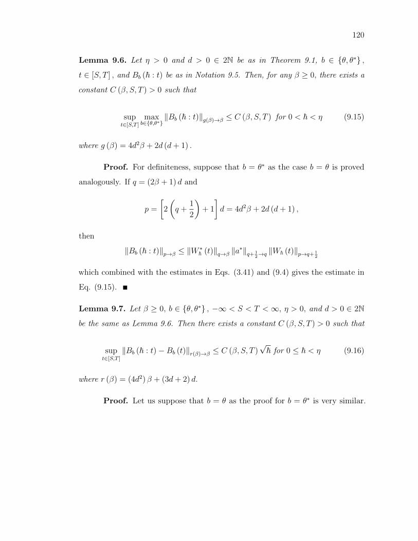
120

Lemma 9.6. Let η > 0 and d > 0 ∈ 2N be as in Theorem 9.1, b ∈ θ, θ∗ ,

t ∈ [S, T ] , and Bb (~ : t) be as in Notation 9.5. Then, for any β ≥ 0, there exists a

constant C (β, S, T ) > 0 such that

supt∈[S,T ]

maxb∈θ,θ∗

‖Bb (~ : t)‖g(β)→β ≤ C (β, S, T ) for 0 < ~ < η (9.15)

where g (β) = 4d2β + 2d (d+ 1) .

Proof. For definiteness, suppose that b = θ∗ as the case b = θ is proved

analogously. If q = (2β + 1) d and

p =

[2

(q +

1

2

)+ 1

]d = 4d2β + 2d (d+ 1) ,

then

‖Bb (~ : t)‖p→β ≤ ‖W∗~ (t)‖q→β ‖a

∗‖q+ 12→q ‖W~ (t)‖p→q+ 1

2

which combined with the estimates in Eqs. (3.41) and (9.4) gives the estimate in

Eq. (9.15).

Lemma 9.7. Let β ≥ 0, b ∈ θ, θ∗ , −∞ < S < T <∞, η > 0, and d > 0 ∈ 2N

be the same as Lemma 9.6. Then there exists a constant C (β, S, T ) > 0 such that

supt∈[S,T ]

‖Bb (~ : t)−Bb (t)‖r(β)→β ≤ C (β, S, T )√~ for 0 ≤ ~ < η (9.16)

where r (β) = (4d2) β + (3d+ 2) d.

Proof. Let us suppose that b = θ as the proof for b = θ∗ is very similar.

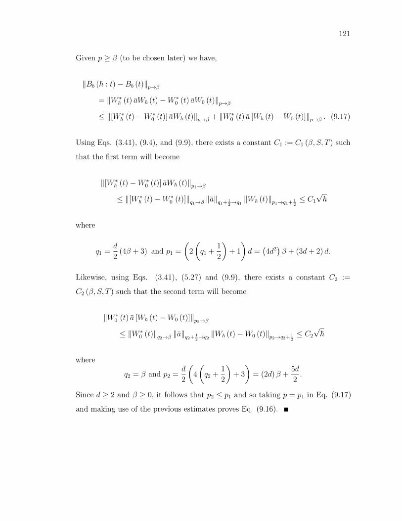
121

Given p ≥ β (to be chosen later) we have,

‖Bb (~ : t)−Bb (t)‖p→β

= ‖W ∗~ (t) aW~ (t)−W ∗

0 (t) aW0 (t)‖p→β

≤ ‖[W ∗~ (t)−W ∗

0 (t)] aW~ (t)‖p→β + ‖W ∗0 (t) a [W~ (t)−W0 (t)]‖p→β . (9.17)

Using Eqs. (3.41), (9.4), and (9.9), there exists a constant C1 := C1 (β, S, T ) such

that the first term will become

‖[W ∗~ (t)−W ∗

0 (t)] aW~ (t)‖p1→β

≤ ‖[W ∗~ (t)−W ∗

0 (t)]‖q1→β ‖a‖q1+ 12→q1 ‖W~ (t)‖p1→q1+ 1

2≤ C1

√~

where

q1 =d

2(4β + 3) and p1 =

(2

(q1 +

1

2

)+ 1

)d =

(4d2)β + (3d+ 2) d.

Likewise, using Eqs. (3.41), (5.27) and (9.9), there exists a constant C2 :=

C2 (β, S, T ) such that the second term will become

‖W ∗0 (t) a [W~ (t)−W0 (t)]‖p2→β

≤ ‖W ∗0 (t)‖q2→β ‖a‖q2+ 1

2→q2 ‖W~ (t)−W0 (t)‖p2→q2+ 1

2≤ C2

√~

where

q2 = β and p2 =d

2

(4

(q2 +

1

2

)+ 3

)= (2d) β +

5d

2.

Since d ≥ 2 and β ≥ 0, it follows that p2 ≤ p1 and so taking p = p1 in Eq. (9.17)

and making use of the previous estimates proves Eq. (9.16).

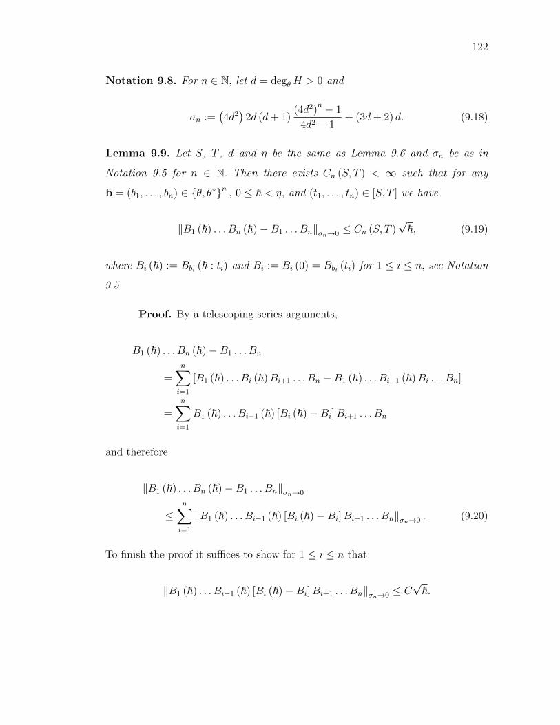
122

Notation 9.8. For n ∈ N, let d = degθH > 0 and

σn :=(4d2)

2d (d+ 1)(4d2)

n − 1

4d2 − 1+ (3d+ 2) d. (9.18)

Lemma 9.9. Let S, T , d and η be the same as Lemma 9.6 and σn be as in

Notation 9.5 for n ∈ N. Then there exists Cn (S, T ) < ∞ such that for any

b = (b1, . . . , bn) ∈ θ, θ∗n , 0 ≤ ~ < η, and (t1, . . . , tn) ∈ [S, T ] we have

‖B1 (~) . . . Bn (~)−B1 . . . Bn‖σn→0 ≤ Cn (S, T )√~, (9.19)

where Bi (~) := Bbi (~ : ti) and Bi := Bi (0) = Bbi (ti) for 1 ≤ i ≤ n, see Notation

9.5.

Proof. By a telescoping series arguments,

B1 (~) . . . Bn (~)−B1 . . . Bn

=n∑i=1

[B1 (~) . . . Bi (~)Bi+1 . . . Bn −B1 (~) . . . Bi−1 (~)Bi . . . Bn]

=n∑i=1

B1 (~) . . . Bi−1 (~) [Bi (~)−Bi]Bi+1 . . . Bn

and therefore

‖B1 (~) . . . Bn (~)−B1 . . . Bn‖σn→0

≤n∑i=1

‖B1 (~) . . . Bi−1 (~) [Bi (~)−Bi]Bi+1 . . . Bn‖σn→0 . (9.20)

To finish the proof it suffices to show for 1 ≤ i ≤ n that

‖B1 (~) . . . Bi−1 (~) [Bi (~)−Bi]Bi+1 . . . Bn‖σn→0 ≤ C√~.

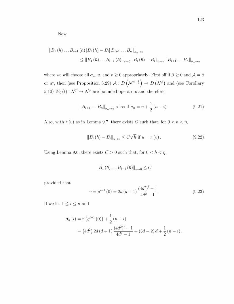
123

Now

‖B1 (~) . . . Bi−1 (~) [Bi (~)−Bi]Bi+1 . . . Bn‖σn→0

≤ ‖B1 (~) . . . Bi−1 (~)‖v→0 ‖Bi (~)−Bi‖u→v ‖Bi+1 . . . Bn‖σn→u

where we will choose all σn, u, and v ≥ 0 appropriately. First off if β ≥ 0 and A = a

or a∗, then (see Proposition 3.29) A : D(N β+ 1

2

)→ D

(N β)

and (see Corollary

5.10) W0 (t) : N β → N β are bounded operators and therefore,

‖Bi+1 . . . Bn‖σn→u <∞ if σn = u+1

2(n− i) . (9.21)

Also, with r (v) as in Lemma 9.7, there exists C such that, for 0 < ~ < η,

‖Bi (~)−Bi‖u→v ≤ C√~ if u = r (v) . (9.22)

Using Lemma 9.6, there exists C > 0 such that, for 0 < ~ < η,

‖B1 (~) . . . Bi−1 (~)‖v→0 ≤ C

provided that

v = gi−1 (0) = 2d (d+ 1)(4d2)

i − 1

4d2 − 1. (9.23)

If we let 1 ≤ i ≤ n and

σn (i) = r(gi−1 (0)

)+

1

2(n− i)

=(4d2)

2d (d+ 1)(4d2)

i − 1

4d2 − 1+ (3d+ 2) d+

1

2(n− i) ,

124

then the by the above bounds it follows that

‖B1 (~) . . . Bi−1 (~) [Bi (~)−Bi]Bi+1 . . . Bn‖σn(i)→0 <∞. (9.24)

One shows σn (i) is increasing in i and therefore max1≤i≤n σn (i) = σn (n) = σn

where σn is as in Notation 9.8. Equation (9.19) now follows from Eqs. (9.20) and

(9.24) with σn (i) increased to σn.

We finish the proof of Theorem 1.17 with Lemma 9.9.

Proof of Theorem 1.17. Note that we have already shown that A~ (ti)

and A†~ (ti) preserve S from Eq. (6.1) and U~ (α0)S = S and U~ (α0)∗ S = S from

Proposition 2.4. To show Eq.(1.23), for ψ ∈ S, we have

⟨P(A~ (ti)− α (ti) , A

†~ (ti)− α (ti)

ni=1

)⟩U~(α0)ψ

=⟨P(U∗~ (α0)A~ (ti)U~ (α0)− α (ti) , U

∗~ (α0)A†~ (ti)U~ (α0)− α (ti)

ni=1

)⟩ψ

=⟨P(√

~a (~ : ti) ,√~a† (~ : ti)

ni=1

)⟩ψ

(9.25)

where 〈·〉ψ is defined in Definition 1.7 and the last step is asserted by Eq. (9.14).

Supposed p = deg (P (θ, θ∗ni=1)) and pmin is then minimum degree of each non-

constant term in P (θi, θ∗i ni=1) . As p = 0 is a trivial case, we assume p > 0. Then,

it follows

P (θi, θ∗i ni=1) = P0 +

p∑k=pmin

Pk (θi, θ∗i ni=1) (9.26)

where P0 ∈ C and

Pk (θi, θ∗i ni=1) =

∑b1,....,bk∈θi,θ∗i ni=1

c (b1, . . . , bk) b1 . . . bk

is a homogeneous polynomial of θi, θ∗i ni=1 with degree k. Plugging Eq.(9.26) into

125

Eq.(9.25) gives,

⟨P(√

~a (~ : ti) ,√~a† (~ : ti)

ni=1

)⟩ψ

=P0 +

p∑k=pmin

~k2

⟨Pk(a (~ : ti) , a

† (~ : ti)ni=1

)⟩ψ

(9.27)

wherein we have used the fact that Pk is a homogeneous polynomial of degree k in

θi, θ∗i ni=1 . By Lemma 9.9, for 0 < ~ < η, we have

∥∥Pk (a (~ : ti) , a† (~ : ti)

ni=1

)ψ∥∥ =

∥∥Pk (a (ti) , a† (ti)

ni=1

)ψ∥∥+O

(√~).

Therefore, for k ≥ 1, we have

~k2

⟨Pk(a (~ : ti) , a

† (~ : ti)ni=1

)⟩ψ

= ~k2

⟨Pk(a (ti) , a

† (ti)ni=1

)⟩ψ

+O(~k+12

). (9.28)

Applying Eq.(9.28) to Eq.(9.27), we have

⟨P(√

~a (~ : ti) ,√~a† (~ : ti)

ni=1

)⟩ψ

= P0 +

p∑k=pmin

~k2

⟨Pk(a (ti) , a

† (ti)ni=1

)⟩ψ

+O(~k+12

)=⟨P(√

~a (ti) ,√~a† (ti)

ni=1

)⟩ψ

+O(~pmin+1

2

).

Therefore, Eq.(1.23) follows immediately.

2 Proof of Corollary 1.19

Let P (θi, θ∗i ni=1) ∈ C 〈θi, θ∗i

ni=1〉 be a non-commutative polynomial, ψ ∈

S and t1, . . . , tn ⊆ R. With out loss of generality, we assume deg (P ) ≥ 1. We

126

define, (may see Notation 2.16),

P (α (ti) : θi, θ∗i ni=1) = P (θi + α (ti) , θ

∗i + α (ti)ni=1)

∈ C[α (ti) , α (ti)

ni=1

]〈θi, θ∗i

ni=1〉 .

Note that degθ

(P)

= deg (P ) (see Notation 2.16) and pmin ≥ 1 because deg(P)≥

1. By Theorem 1.17 , for 0 < ~ < η, we have

⟨P(A~ (ti) , A

†~ (ti)

ni=1

)⟩U~(α0)ψ

=⟨P(α (ti) : A~ (ti)− α (ti) , A

†~ (ti)− α (ti)

ni=1

)⟩U~(α0)ψ

=⟨P(α (ti) :

√~a (ti) ,

√~a† (ti)

ni=1

)⟩ψ

+O(~pmin+1

2

)=⟨P(α (ti) +

√~a (ti) , α (ti) +

√~a† (ti)

ni=1

)⟩ψ

+O(~pmin+1

2

)=⟨P(α (ti) +

√~a (ti) , α (ti) +

√~a† (ti)

ni=1

)⟩ψ

+O (~) .

The last equality is because pmin is at least 1. Therefore, Eq. (1.25) follows.

3 Proof of Corollary 1.21

By Eqs. (1.8) and (1.9) in Definition 1.3, the term⟨P1

(α (ti) : a (ti) , a

† (ti)ni=1

)⟩ψ

in Eq.(1.26) is bounded independent of ~ for ψ ∈ S. Therefore, by setting ~→ 0 in

Eq.(1.26), Eq.(1.28) follows. To show Eq.(1.29), let pmin be the minimum degree of

all non constant terms in P (θi, θ∗i ni=1) . We assume pmin ≥ 1 as usual. Otherwise,

it means P is a constant polynomial which is a trivial case in Eq. (1.29). With the

same notations as in Eq. (9.26), we have

P (θi, θ∗i ni=1) = P0 +

p∑k=pmin

Pk (θi, θ∗i ni=1) .

127

Then, we apply Eq.(1.23) on each term Pk where k ≥ 1, and get

⟨Pk

(A~ (ti)− α (ti) , A

†~ (ti)− α (ti)

ni=1

)⟩U~(α0)ψ

=⟨Pk

(√~a (ti) ,

√~a† (ti)

ni=1

)⟩ψ

+O(~k+12

)=~

k2

(⟨Pk(a (ti) , a

† (ti)ni=1

)⟩ψ

+O(~

12

)). (9.29)

By applying Eq.(9.29), we have

⟨P

(A~ (ti)− α (ti)√

~,A†~ (ti)− α (ti)√

~

n

i=1

)⟩U~(α0)ψ

= P0 +

p∑k=pmin

1

~ k2

⟨Pk

(A~ (ti)− α (ti) , A

†~ (ti)− α (ti)

ni=1

)⟩U~(α0)ψ

= P0 +

p∑k=pmin

⟨Pk(a (ti) , a

† (ti)ni=1

)⟩ψ

+O(~

12

)=⟨P(a (ti) , a

† (ti)ni=1

)⟩ψ

+O(~

12

).

Eq.(1.29) follows.

Part II

Powers of Symmetric Differential

Operators

128

Chapter 10

A Structure Theorem for

Symmetric Differential Operators

Remark 10.1. It is useful to observe if A and B are two linear transformation

from a vector space, V, to itself, then

AB2 +B2A = 2BAB + [B, [B,A]] ,

where [A,B] := AB −BA denotes the commutator of A and B.

Proposition 10.2. Suppose akdk=0 ⊂ C∞ (R,R) and L is the dth -order differ-

ential operator on C∞(R) as defined in Eq. (1.30). If L is symmetric according

to Definition 1.26 (i.e. L = L† where L† is as in Eq. (1.32)), then d is even (let

m = d/2) and there exists blml=0 ⊂ C∞ (R,R) such that

L =m∑l=0

(−1)l ∂lMbl∂l (10.1)

where Mbl is as in Notation 1.24. Moreover, bm = (−1)m a2m = (−1)m ad.

129

130

Proof. Since L = L†, we have

L =1

2(L+ L†) =

1

2

d∑k=0

[ak∂k + (−1)k∂kMak ] (10.2)

=1

2[ad∂

d + (−1)d∂dMad ] + [diff. operator of order d− 1]. (10.3)

If d were odd, then (−1)d = −1 and hence (using the product rule),

1

2[ad∂

d + (−1)d∂dMad ] =1

2[Mad , ∂

d]

= [diff. operator of order d− 1]

which combined with Eq. (10.3) would imply that L was in fact a differential

operator of order no greater than d− 1. This shows that L must be an even order

operator.

Now knowing that d is even, let m := d/2 ∈ N. From Eq. (10.2), we learn

that

L =1

2

2m∑k=0

[ak∂

k + (−1)k ∂kMak

]=

1

2

[a2m∂

2m + ∂2mMa2m

]+R

where R is given by

R =1

2

2m−1∑k=0

[Mak∂

k + (−1)k ∂kMak

].

Moreover by Remark 1.27, R is still symmetric. As in the previous paragraph R is

in fact an even order differential operator and its order is at most 2m− 2. Using

131

Remark 10.1 with A = Ma2m , B = ∂m, and V = C∞ (R) , we learn that

1

2

[a2m∂

2m + ∂2mMa2m

]= ∂mMa2m∂

m +1

2[∂m, [∂m,Ma2m ]]

= ∂mMa2m∂m + [diff. operator of order at most 2m− 2].

Combining the last three displayed equations together shows

L = ∂ma2m∂m + S

where S = L− ∂ma2m∂m is a symmetric (by Remark 1.27) even order differential

operator or at most 2m− 2. It now follows by the induction hypothesis that

S =m−1∑l=0

(−1)l ∂lMbl∂l =⇒ L =

m∑l=0

(−1)l ∂lMbl∂l

where bm := (−1)m a2m.

Our next goal is to record the explicit relationship between ak2mk=0 in

Eq. (1.30) and bkmk=0 in Eq. (10.1).

Convention 10.3. To simplify notation in what follows, for k, l ∈ Z, let

(l

k

):=

l!

k!(l−k)!if 0 ≤ k ≤ l

0 otherwise.

Lemma 10.4. If ak2mk=0 ∪ bl

ml=0 ⊂ C∞ (R,R) and

m∑l=0

(−1)l ∂lbl (x) ∂l =2m∑k=0

ak (x) ∂k , (10.4)

then

ak :=m∑l=0

(l

k − l

)(−1)l ∂2l−kbl. (10.5)

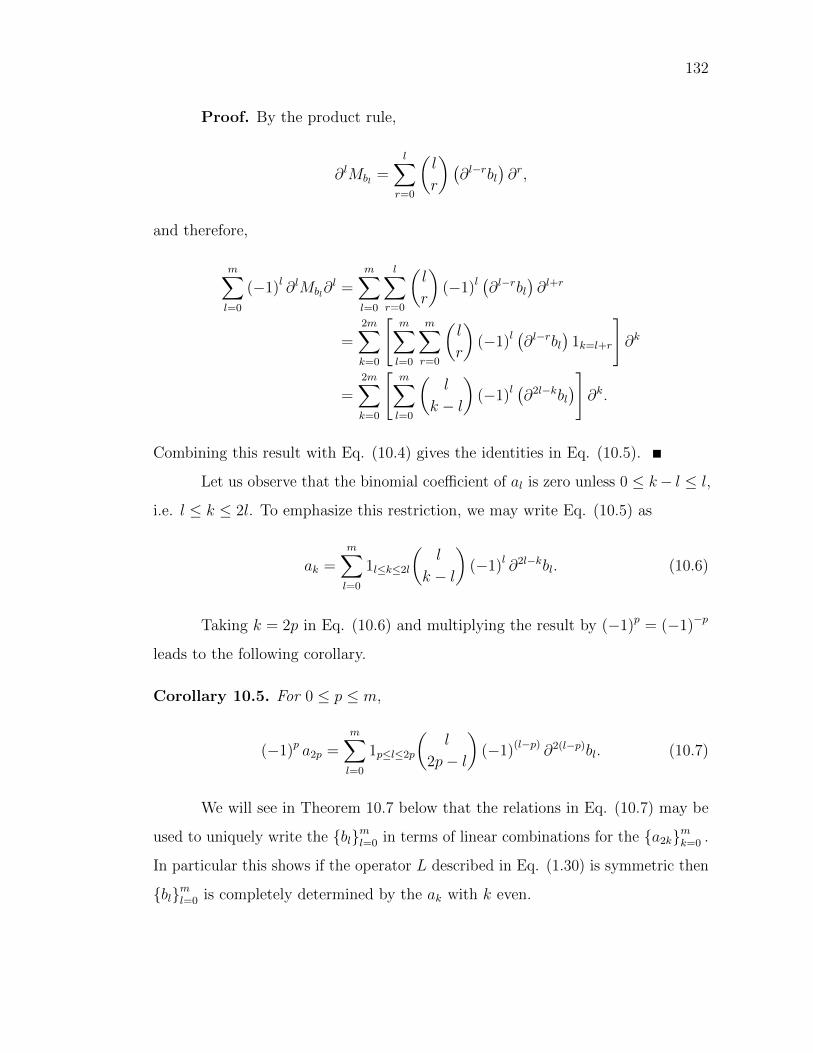
132

Proof. By the product rule,

∂lMbl =l∑

r=0

(l

r

)(∂l−rbl

)∂r,

and therefore,

m∑l=0

(−1)l ∂lMbl∂l =

m∑l=0

l∑r=0

(l

r

)(−1)l

(∂l−rbl

)∂l+r

=2m∑k=0

[m∑l=0

m∑r=0

(l

r

)(−1)l

(∂l−rbl

)1k=l+r

]∂k

=2m∑k=0

[m∑l=0

(l

k − l

)(−1)l

(∂2l−kbl

)]∂k.

Combining this result with Eq. (10.4) gives the identities in Eq. (10.5).

Let us observe that the binomial coefficient of al is zero unless 0 ≤ k− l ≤ l,

i.e. l ≤ k ≤ 2l. To emphasize this restriction, we may write Eq. (10.5) as

ak =m∑l=0

1l≤k≤2l

(l

k − l

)(−1)l ∂2l−kbl. (10.6)

Taking k = 2p in Eq. (10.6) and multiplying the result by (−1)p = (−1)−p

leads to the following corollary.

Corollary 10.5. For 0 ≤ p ≤ m,

(−1)p a2p =m∑l=0

1p≤l≤2p

(l

2p− l

)(−1)(l−p) ∂2(l−p)bl. (10.7)

We will see in Theorem 10.7 below that the relations in Eq. (10.7) may be

used to uniquely write the blml=0 in terms of linear combinations for the a2kmk=0 .

In particular this shows if the operator L described in Eq. (1.30) is symmetric then

blml=0 is completely determined by the ak with k even.

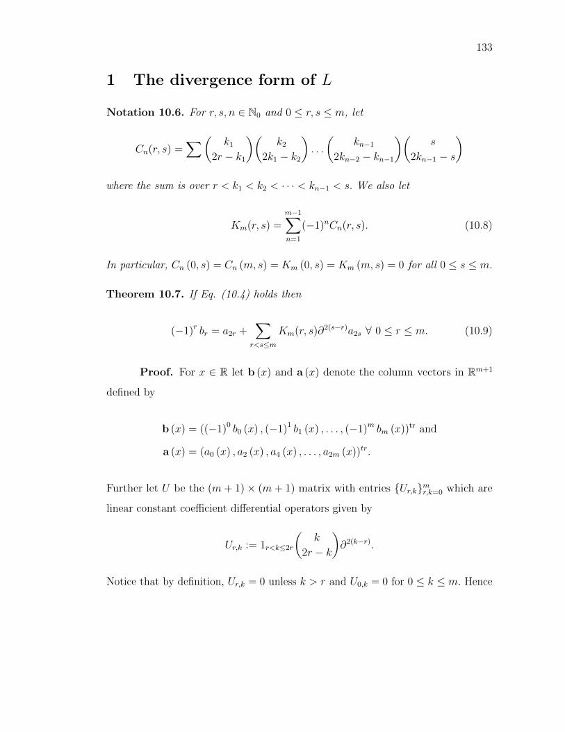
133

1 The divergence form of L

Notation 10.6. For r, s, n ∈ N0 and 0 ≤ r, s ≤ m, let

Cn(r, s) =∑(

k1

2r − k1

)(k2

2k1 − k2

). . .

(kn−1

2kn−2 − kn−1

)(s

2kn−1 − s

)

where the sum is over r < k1 < k2 < · · · < kn−1 < s. We also let

Km(r, s) =m−1∑n=1

(−1)nCn(r, s). (10.8)

In particular, Cn (0, s) = Cn (m, s) = Km (0, s) = Km (m, s) = 0 for all 0 ≤ s ≤ m.

Theorem 10.7. If Eq. (10.4) holds then

(−1)r br = a2r +∑

r<s≤m

Km(r, s)∂2(s−r)a2s ∀ 0 ≤ r ≤ m. (10.9)

Proof. For x ∈ R let b (x) and a (x) denote the column vectors in Rm+1

defined by

b (x) = ((−1)0 b0 (x) , (−1)1 b1 (x) , . . . , (−1)m bm (x))tr and

a (x) = (a0 (x) , a2 (x) , a4 (x) , . . . , a2m (x))tr.

Further let U be the (m+ 1)× (m+ 1) matrix with entries Ur,kmr,k=0 which are

linear constant coefficient differential operators given by

Ur,k := 1r<k≤2r

(k

2r − k

)∂2(k−r).

Notice that by definition, Ur,k = 0 unless k > r and U0,k = 0 for 0 ≤ k ≤ m. Hence

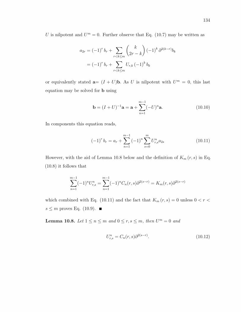
134

U is nilpotent and Um = 0. Further observe that Eq. (10.7) may be written as

a2r = (−1)r br +∑

r<k≤m

(k

2r − k

)(−1)k ∂2(k−r)bk

= (−1)r br +∑

r<k≤m

Ur,k (−1)k bk

or equivalently stated a= (I + U)b. As U is nilpotent with Um = 0, this last

equation may be solved for b using

b = (I + U)−1a = a +m−1∑n=1

(−U)na. (10.10)

In components this equation reads,

(−1)r br = ar +m−1∑n=1

(−1)nm∑s=0

Unr,sa2s (10.11)

However, with the aid of Lemma 10.8 below and the definition of Km (r, s) in Eq.

(10.8) it follows that

m−1∑n=1

(−1)nUnr,s =

m−1∑n=1

(−1)nCn(r, s)∂2(s−r) = Km(r, s)∂2(s−r)

which combined with Eq. (10.11) and the fact that Km (r, s) = 0 unless 0 < r <

s ≤ m proves Eq. (10.9).

Lemma 10.8. Let 1 ≤ n ≤ m and 0 ≤ r, s ≤ m, then Um = 0 and

Unr,s = Cn(r, s)∂2(s−r). (10.12)

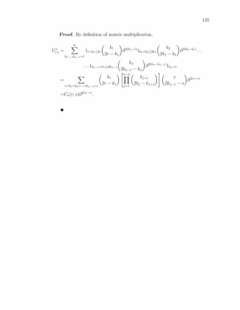
135

Proof. By definition of matrix multiplication,

Unr,s =

m∑k1,...,kn−1=1

1r<k1≤2r

(k1

2r − k1

)∂2(k1−r)1k1<k2≤2k1

(k2

2k1 − k2

)∂2(k2−k1) . . .

. . . 1kn−1<kn≤2kn−1

(kn

2kn−1 − kn

)∂2(kn−kn−1)1kn=s

=∑

r<k1<k2<···<kn−1<s

(k1

2r − k1

)[n−2∏j=1

(kj+1

2kj − kj+1

)](s

2kn−1 − s

)∂2(s−r)

=Cn(r, s)∂2(s−r).

Chapter 11

The structure of Ln

In this chapter let us fix a 2m – order symmetric differential operator, L,

acting on C∞(R) which can be written as in both of the equations (1.30) and (10.1)

where the coefficients, ak2mk=0 and blml=0 are all real valued smooth functions

on R. If n ∈ N, Ln is a 2mn – order symmetric linear differential operator on

C∞ (R) and hence there exists Ak2mnk=0 ⊂ C∞ (R,R) and (using Proposition 10.2)

Blmnl=0 ⊂ C∞ (R,R) such that

Ln =2mn∑k=0

Ak∂k =

mn∑`=0

(−1)` ∂`B`∂`. (11.1)

Our goal in this chapter is to compute the coefficients Ak2mnk=0 in terms of

the coefficients blml=0 defining L as in Eq. (10.1). It turns out that it is useful

to compare Ln to the operators which is constructed by writing out Ln while

pretending that the coefficients ak2mk=0 or blml=0 are constant. This is explained

in the following notations.

Notation 11.1. For n ∈ N and m ∈ N, let Λm := 0, 1, . . . ,m ⊂ N0 and for

j = (j1, . . . , jn) ∈ Λnm, let |j| = j1 + j2 + · · ·+ jn. If k = (k1, . . . , kn) ∈ Λn

m is another

multi-index, we write k ≤ j to mean ki ≤ ji for 1 ≤ i ≤ n. [We will use this

136

137

notation when m =∞ as well in which case Λ∞ = N0.]

Notation 11.2. Given n ∈ N, and L as in Eq. (10.1), let B`mn`=0 be C∞ (R,R) –

functions defined by

B` :=∑j∈Λnm

1|j|=`bj1 . . . bjn (11.2)

and L(n)B be the differential operator given by

L(n)B :=

nm∑`=0

(−1)` ∂`B`∂`. (11.3)

It will also be convenient later to set Bk/2 ≡ 0 when k is an odd integer.

Example 11.3. If m = 1 and n = 2, then

L = −∂b1∂ + b0 and

L2 = ∂b1∂2b1∂ − ∂b1∂b0 − b0∂b1∂ + b2

0.

To put L2 into divergence form we repeatedly use the product rule, ∂V = V ∂ + V ′.

Thus

∂b1∂b0 + b0∂b1∂ = ∂b1b0∂ + ∂b1b′0 + ∂b0b1∂ − b′0b1∂

= 2∂b1b0∂ + (b1b′0)′

and

∂b1∂2b1∂ = ∂2b1∂b1∂ − ∂b′1∂b1∂

= ∂2b1b1∂2 + ∂2b1b

′1∂ − ∂b′1b′1∂ − ∂b′1b1∂

2

= ∂2b1b1∂2 + ∂ (b1b

′1)′∂ − ∂b′1b′1∂.

138

Combining the last three displayed equations together shows

L2 = ∂2b21∂

2 + ∂[−2b1b0 + (b1b

′1)′ − (b′1)

2]∂ + b2

0 − (b1b′0)′

= ∂2b21∂

2 + ∂ [−2b1b0 + b1b′′1] ∂ + b2

0 − (b1b′0)′. (11.4)

Dropping all terms in Eq. (11.4) which contain a derivative of b1 or b0 shows

L(2)B = ∂2b2

1∂2 − ∂ [2b0b1] ∂ + b2

0. (11.5)

Notation 11.4. For j ∈ Nn0 and k ∈ Nn

0 , let

(k

j

):=

n∏i=1

(kiji

)

where the binomial coefficients are as in Convention 10.3.

Lemma 11.5. If L is as in Eq. (10.1),

Me−iξ(·)LMeiξ(·) =m∑l=0

(−1)l (∂ + iξ)lMbl(·) (∂ + iξ)l . (11.6)

Proof. If f ∈ C∞ (R) , the product rule gives,

∂x[eiξxf (x)

]= eiξx (∂x + iξ) f (x) ,

which is to say,

Me−iξ(·)∂Meiξ(·) = (∂ + iξ) . (11.7)

Combining Eq. (11.7) with the fact that

Me−iξ(·)MblMeiξ(·) = Mbl

139

allows us to conclude,

Me−iξ(·)LMeiξ(·) =m∑l=0

(−1)lMe−iξ(·)∂lMbl∂

lMeiξ(·)

=m∑l=0

(−1)lMe−iξ(·)∂lMeiξ(·)MblMe−iξ(·)∂

lMeiξ(·)

=m∑l=0

(−1)l (∂ + iξ)lMbl(·) (∂ + iξ)l .

Notation 11.6. For q, l, j ∈Λnm, let

Ck (q, l, j) := (−1)|q|(

q

l

)(q

j

)1j1=012|q|−k=|l|+|j|>0, (11.8)

and for k ∈ Λ2m let

Tk :=∑

q,l,j∈Λnm

Ck (q, l, j)(∂lnMbqn∂

jn) (∂ln−1Mbqn−1

∂jn−1

). . .(∂l1Mbq1

∂j1)

1 (11.9)

where 1 is a function constantly equal to 1. We will often abuse notation and write

this last equation as,

Tk (x) :=∑

q,l,j∈Λnm

Ck (q, l, j)(∂lnx bqn (x) ∂jnx

). . .(∂l2x bq2∂

j2x

)∂l1x bq1 (x) .

Proposition 11.7 (Ak = Ak (blml=0)). If L is given as in Eq. (10.1), then

coefficients Ak2mnk=0 of Ln in Eq. (11.1) are given by

Ak = 1k∈2N0 · (−1)k/2 Bk/2 + Tk, (11.10)

where B` and Tk are as in Notations 11.2 and 11.6 respectively. Moreover, if we

140

further assume blml=0 are polynomial functions such that

deg (bl) ≤ max deg (b0) , 0 for 1 ≤ ` ≤ m, (11.11)

then B`mn`=0 and Tk2mnk=0 are polynomials such that

deg (Tk) < max n deg (b0) , 0 = max deg (B0) , 0 for 0 ≤ k ≤ 2mn.

Proof. First observe that if Ln is described as in Eq. (11.1), then

2mn∑k=0

Ak (x) (iξ)k = σn (x, ξ) = e−iξxLnx(eiξx)

where σn := σLn is a symbol of Ln defined in Eq. (1.31) and Lnx is a differential

operator with respect to x. To compute the right side of this equation, take the nth

– power of Eq. (11.6) to learn

Me−iξ(·)LnMeiξ(·) = (Me−iξ(·)LMeiξ(·))

n

=m∑

q1,...,qn=0

(∂ + iξ)qn (−1)qnMbqn (∂ + iξ)qn . . . (∂ + iξ)q1 (−1)q1 Mbq1(∂ + iξ)q1

=∑

q∈Λm

(−1)|q| (∂ + iξ)qnMbqn (∂ + iξ)qn . . . (∂ + iξ)q1 Mbq1(∂ + iξ)q1 .

Applying this result to the constant function 1 then shows

σn (x, ξ) = e−iξxLnx(eiξx)

= Me−iξxLnxMeiξx1

=∑

q∈Λm

(−1)|q| (∂ + iξ)qnMbqn (∂ + iξ)qn . . . (∂ + iξ)q1 Mbq1(∂ + iξ)q1 1.

Making repeatedly used of the binomial formula to expand out all the terms

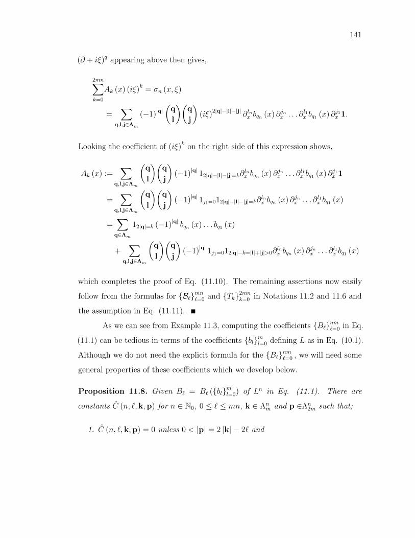
141

(∂ + iξ)q appearing above then gives,

2mn∑k=0

Ak (x) (iξ)k = σn (x, ξ)

=∑

q,l,j∈Λm

(−1)|q|(

q

l

)(q

j

)(iξ)2|q|−|l|−|j| ∂lnx bqn (x) ∂jnx . . . ∂l1x bq1 (x) ∂j1x 1.

Looking the coefficient of (iξ)k on the right side of this expression shows,

Ak (x) :=∑

q,l,j∈Λm

(q

l

)(q

j

)(−1)|q| 12|q|−|l|−|j|=k∂

lnx bqn (x) ∂jnx . . . ∂l1x bq1 (x) ∂j1x 1

=∑

q,l,j∈Λm

(q

l

)(q

j

)(−1)|q| 1j1=012|q|−|l|−|j|=k∂

lnx bqn (x) ∂jnx . . . ∂l1x bq1 (x)

=∑

q∈Λm

12|q|=k (−1)|q| bqn (x) . . . bq1 (x)

+∑

q,l,j∈Λm

(q

l

)(q

j

)(−1)|q| 1j1=012|q|−k=|l|+|j|>0∂

lnx bqn (x) ∂jnx . . . ∂l1x bq1 (x)

which completes the proof of Eq. (11.10). The remaining assertions now easily

follow from the formulas for B`mn`=0 and Tk2mnk=0 in Notations 11.2 and 11.6 and

the assumption in Eq. (11.11).

As we can see from Example 11.3, computing the coefficients B`nm`=0 in Eq.

(11.1) can be tedious in terms of the coefficients blml=0 defining L as in Eq. (10.1).

Although we do not need the explicit formula for the B`nm`=0 , we will need some

general properties of these coefficients which we develop below.

Proposition 11.8. Given B` = B` (blml=0) of Ln in Eq. (11.1). There are

constants C (n, `,k,p) for n ∈ N0, 0 ≤ ` ≤ mn, k ∈ Λnm and p ∈Λn

2m such that;

1. C (n, `,k,p) = 0 unless 0 < |p| = 2 |k| − 2` and

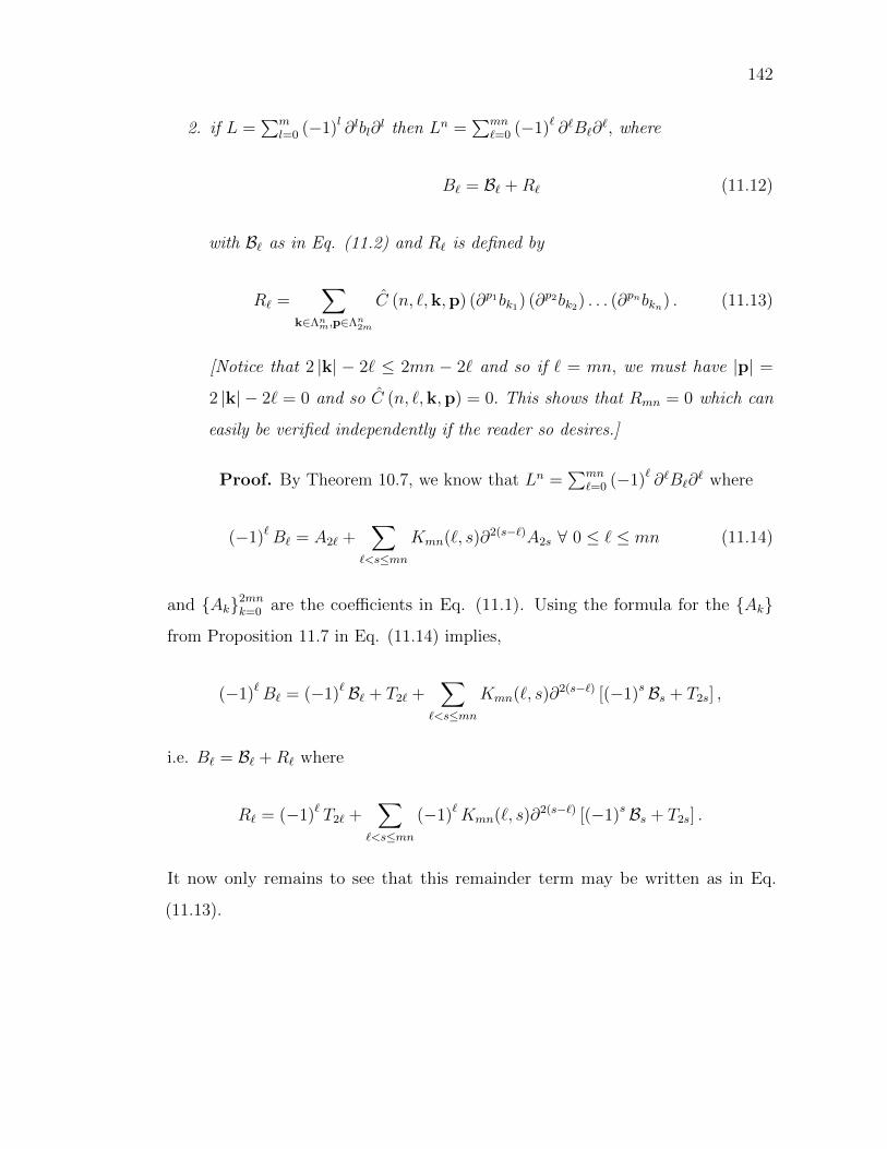
142

2. if L =∑m

l=0 (−1)l ∂lbl∂l then Ln =

∑mn`=0 (−1)` ∂`B`∂

`, where

B` = B` +R` (11.12)

with B` as in Eq. (11.2) and R` is defined by

R` =∑

k∈Λnm,p∈Λn2m

C (n, `,k,p) (∂p1bk1) (∂p2bk2) . . . (∂pnbkn) . (11.13)

[Notice that 2 |k| − 2` ≤ 2mn − 2` and so if ` = mn, we must have |p| =

2 |k| − 2` = 0 and so C (n, `,k,p) = 0. This shows that Rmn = 0 which can

easily be verified independently if the reader so desires.]

Proof. By Theorem 10.7, we know that Ln =∑mn

`=0 (−1)` ∂`B`∂` where

(−1)`B` = A2` +∑

`<s≤mn

Kmn(`, s)∂2(s−`)A2s ∀ 0 ≤ ` ≤ mn (11.14)

and Ak2mnk=0 are the coefficients in Eq. (11.1). Using the formula for the Ak

from Proposition 11.7 in Eq. (11.14) implies,

(−1)`B` = (−1)` B` + T2` +∑

`<s≤mn

Kmn(`, s)∂2(s−`) [(−1)s Bs + T2s] ,

i.e. B` = B` +R` where

R` = (−1)` T2` +∑

`<s≤mn

(−1)`Kmn(`, s)∂2(s−`) [(−1)s Bs + T2s] .

It now only remains to see that this remainder term may be written as in Eq.

(11.13).

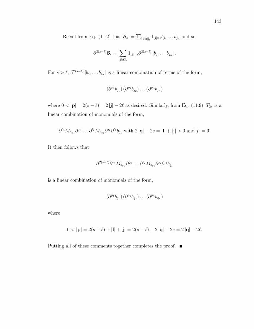
143

Recall from Eq. (11.2) that Bs :=∑

j∈Λnm1|j|=sbj1 . . . bjn and so

∂2(s−`)Bs =∑j∈Λnm

1|j|=s∂2(s−`) [bj1 . . . bjn ] .

For s > `, ∂2(s−`) [bj1 . . . bjn ] is a linear combination of terms of the form,

(∂p1bj1) (∂p2bj2) . . . (∂pnbjn)

where 0 < |p| = 2(s− `) = 2 |j| − 2` as desired. Similarly, from Eq. (11.9), T2s is a

linear combination of monomials of the form,

∂lnMbqn∂jn . . . ∂l2Mbq2

∂j2∂l1bq1 with 2 |q| − 2s = |l|+ |j| > 0 and j1 = 0.

It then follows that

∂2(s−`)∂lnMbqn∂jn . . . ∂l2Mbq2

∂j2∂l1bq1

is a linear combination of monomials of the form,

(∂p1bq1) (∂p2bq2) . . . (∂pnbqn)

where

0 < |p| = 2(s− `) + |l|+ |j| = 2(s− `) + 2 |q| − 2s = 2 |q| − 2`.

Putting all of these comments together completes the proof.

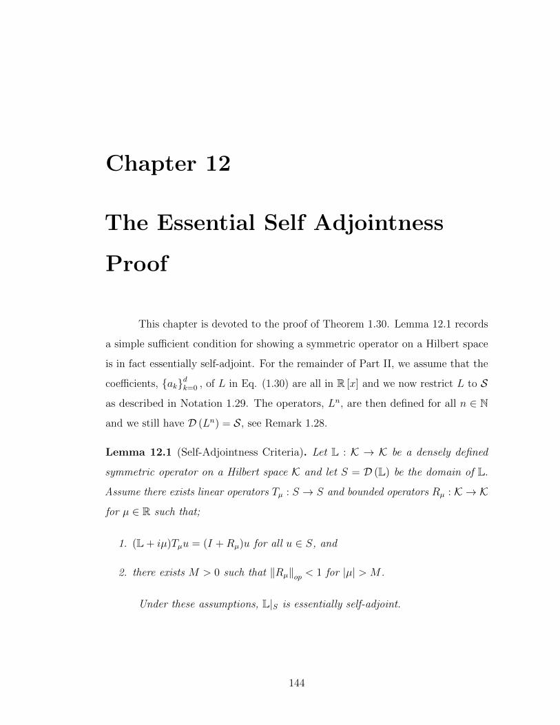
Chapter 12

The Essential Self Adjointness

Proof

This chapter is devoted to the proof of Theorem 1.30. Lemma 12.1 records

a simple sufficient condition for showing a symmetric operator on a Hilbert space

is in fact essentially self-adjoint. For the remainder of Part II, we assume that the

coefficients, akdk=0 , of L in Eq. (1.30) are all in R [x] and we now restrict L to S

as described in Notation 1.29. The operators, Ln, are then defined for all n ∈ N

and we still have D (Ln) = S, see Remark 1.28.

Lemma 12.1 (Self-Adjointness Criteria). Let L : K → K be a densely defined

symmetric operator on a Hilbert space K and let S = D (L) be the domain of L.

Assume there exists linear operators Tµ : S → S and bounded operators Rµ : K → K

for µ ∈ R such that;

1. (L + iµ)Tµu = (I +Rµ)u for all u ∈ S, and

2. there exists M > 0 such that ‖Rµ‖op < 1 for |µ| > M .

Under these assumptions, L|S is essentially self-adjoint.

144

145

Proof. ‖Rµ‖op < 1 for |µ| > M is assumed in condition 2 which implies

I + Rµ is invertible. Therefore, if f ∈ K, then g := (I +Rµ)−1 f ∈ K satisfies

(I +Rµ) g = f. We may then choose gn∞n=1 ⊂ S such that gn → g in K. Let

sn = Tµgn ∈ S. We have, by condition 1, that

‖(L + iµ) sn − f‖ = ‖(I +Rµ)gn − f‖

≤ ||(I +Rµ) (gn − g) ||

≤ ‖I +Rµ‖op ||gn − g|| → 0 as n→∞.

We have thus verified that Ran(L + iµ)|S is dense in K for all |µ| > M from which

it follows that L|S is essentially self-adjoint, see for example the corollary on p.257

in Reed and Simon [32].

Notation 12.2. Let B` (x)mn`=0 be the coefficients defined in Eq. (11.2) and define

Σ (x, ξ) :=mn∑`=0

B` (x) ξ2`. (12.1)

From Eqs. (11.10) and (1.31) the symbol, σn (x, ξ) := σLn (x, ξ) , of Ln

presented as in Eq. (11.1) may be written as

σn (x, ξ) =mn∑`=0

[B` (x) + (−1)` T2` (x)

]ξ2` − i

mn∑`=1

(−1)` T2`−1 (x) ξ2`−1 (12.2)

= Σ (x, ξ) +mn∑`=0

[(−1)` T2` (x)

]ξ2` − i

mn∑`=1

(−1)` T2`−1 (x) ξ2`−1, (12.3)

where the coefficients Tk2mnk=0 are as in Eq. (11.9). More importantly, for our

purposes,

Reσn (x, ξ) = Σ (x, ξ) +mn∑`=0

[(−1)` T2` (x)

]ξ2`. (12.4)

The following lemma will be useful in estimating all of these functions of (x, ξ) .

146

Lemma 12.3. Let 0 ≤ k1 < k2 <∞ and p(x), q(x) and r(x) be real polynomials

such that deg p ≤ deg q, q > 0, and r is bounded from below.

1. If deg (p) < deg (r) or p is a constant function, then, for any k1 < k2 and

λ > 0, there exists cλ such that

∣∣p (x) ξk1∣∣ ≤ λ

(q (x) |ξ|k2 + r (x)

)+ cλ. (12.5)

2. If deg (p) ≤ deg (r) , then for any k1 < k2 and λ > 0, there exists constants

cλ and dλ such that

∣∣p (x) ξk1∣∣ ≤ λq (x) |ξ|k2 + cλr (x) + dλ. (12.6)

Proof. Since deg p ≤ deg q and q > 0, deg q ∈ 2N0 andK := supx∈R |p (x)| /q (x) <

∞, i.e. p (x) ≤ Kq (x) . One also has for every τ > 0, there exists 0 < aτ <∞ such

that∣∣ξk1∣∣ ≤ τ |ξ|k2 + aτ . Combining these estimates shows,

∣∣p (x) ξk1∣∣ ≤ τ |p (x)| |ξ|k2 + aτ |p (x)| (12.7)

≤ τKq (x) |ξ|k2 + aτ |p (x)| . (12.8)

If deg p < deg r, for every δ > 0 there exists 0 < bδ < ∞ such that

|p (x)| ≤ δr (x) + bδ which combined with Eq. (12.8) implies

∣∣p (x) ξk1∣∣ ≤ τKq (x) |ξ|k2 + aτ (δr (x) + bδ)

and Eq. (12.5) follows by choosing τ = λ/K and then δ = λ/aτ so that cλ = aτbδ.

If deg p ≤ deg r, then there exists C1, C2 <∞ such that |p (x)| ≤ C1r (x)+C2

which combined with Eq. (12.8) with τ = λ/K shows

∣∣p (x) ξk1∣∣ ≤ λq (x) |ξ|k2 + aλ/K (C1r (x) + C2)

147

from which Eq. (12.6) follows.

With the use of Lemma 12.3, the following Lemma helps us to estimate

the growth of Tk (x) (see Notation 11.6) and its derivatives of Ln in Eq. (11.1) for

0 ≤ k ≤ 2mn

Lemma 12.4. Suppose that blml=0 are polynomials satisfying the assumptions

in Theorem 1.30. Then for each 0 ≤ k ≤ 2mn, β ∈ N0, and δ > 0, there exists

C = C (k, β, δ) <∞ such that

(1 + |ξ|k

)(1 + |x|β

) ∣∣∂βxTk (x)∣∣ ≤ δΣ (x, ξ) + C (k, β, δ) . (12.9)

Proof. If deg b0 ≤ 0, then by condition 2 in Theorem 1.30 it follows that

blml=0 are all constants in which case Tk ≡ 0 and the Lemma is trivial. So for the

rest of the proof we assume deg b0 > 0.

According to Eq. (11.9), Tk may be expressed as a linear combination of

terms of the form, (∂p1bj1) . . . (∂pnbjn) , where j and p are multi-indices such that

2 |j| − k = |p| > 0. If j and p are multi-indices such that 2 |j| − k = |p| > 0 and

(∂p1bj1) . . . (∂pnbjn) 6= 0, then bj1 . . . bjn is strictly positive and

deg (bj1 . . . bjn) ≥ deg [(∂p1bj1) . . . (∂pnbjn)] + |p| > 0.

Given the term, bj1 . . . bjn , appears in B|j|, we conclude that B|j| is strictly positive

and

deg ((∂p1bj1) . . . (∂pnbjn)) < deg (bj1 . . . bjn) ≤ deg

(B|j|).

Moreover from condition 2 in Theorem 1.30, deg bj ≤ deg b0 for all j and therefore

we also have

deg ((∂p1bj1) . . . (∂pnbjn)) < deg (bj1 . . . bjn) ≤ deg (bn0 ) = degB0.

148

Moreover, for any r, β ∈ N0 with r ≤ β we still have

degxr∂βx [(∂p1bj1) . . . (∂

pnbjn)]≤ deg ((∂p1bj1) . . . (∂

pnbjn))

< min

deg(B|j|), deg (B0)

.

Hence by substituting

p (x) = xr∂βx [(∂p1bj1) . . . (∂pnbjn)] , q (x) = B|j| (x) and r (x) = B0 (x)

in Lemma 12.3, for every λ > 0 there exists Cλ <∞ such that

∣∣xr∂βx [(∂p1bj1) . . . (∂pnbjn)] ξk

∣∣ ≤ λ[B|j| (x) ξ2|j| + B0 (x)

]+ Cλ

≤ λ · Σ (x, ξ) + Cλ

and similarly, ∣∣xr∂βx [(∂p1bj1) . . . (∂pnbjn)]

∣∣ ≤ λΣ (x, ξ) + Cλ.

These last two equations with r = 0 and r = β combine to show, for all λ > 0,

there exists Cλ <∞ such that

(1 + |ξ|k

)(1 + |x|β

) ∣∣∂βx [(∂p1bj1) . . . (∂pnbjn)]

∣∣ ≤ 4 (λΣ (x, ξ) + Cλ) .

By using this result in Eq. (11.9), one then sees there is a constant K <∞ such

that (1 + |ξ|k

)(1 + |x|β

) ∣∣∂βxTk (x)∣∣ ≤ KλΣ (x, ξ) +KCλ.

Equation (12.9) now follows by replacing λ by δ/K in the above equation.

The following Lemma is to study the growth of B` (x) (see Notation 11.2)

and its derivatives of Ln in Eq. (11.1) for 0 ≤ l ≤ mn

Lemma 12.5. Again suppose that blml=0 are polynomials satisfying the assump-

149

tions in Theorem 1.30. For all ` ∈ Λmn, and β ∈ N0, there exists C < ∞ such

that ∣∣∂βxB` (x)∣∣ (|ξ|2` + 1

)(|x|β + 1

)≤ CΣ (x, ξ) + C. (12.10)

Moreover, if we assume b0 is not the zero polynomial, then we may drop the second

C in Eq. (12.10), i.e. there exists C <∞ such that

∣∣∂βxB` (x)∣∣ (|ξ|2` + 1

)(|x|β + 1

)≤ CΣ (x, ξ) . (12.11)

Proof. Case 1. If b0 = 0 then by the assumption 2 of Theorem 1.30 each

bl is a constant for 1 ≤ l ≤ m and therefore ∂βxB` (x) = 0 for all β > 0, i.e. B` are

constant for all `. Moreover, if β = 0, from the definition of Σ (x, ξ) in Eq. (12.1) it

follows that B`ξ2` ≤ Σ (x, ξ) and hence

|B` (x)|(|ξ|2` + 1

)= B`

(ξ2` + 1

)≤ Σ (x, ξ) + B`

and so Eq. (12.10) holds with C = max1≤`≤mn max (1,B`) .

Case 2. If b0 6= 0, let us assume B` is not the zero polynomial for otherwise

there is nothing to prove. Since xβ∂βxB` (x) and ∂βxB` (x) both have degree no more

than degB` and B` > 0, we may conclude there exists C <∞ such that

(1 + |x|β

) ∣∣∂βxB` (x)∣∣ =

∣∣∂βxB` (x)∣∣+∣∣xβ∂βxB` (x)

∣∣ ≤ CB` (x) . (12.12)

Multiplying this equation by ξ2` then shows,

(1 + |x|β

) ∣∣∂βxB` (x)∣∣ ξ2` ≤ CB` (x) ξ2` ≤ CΣ (x, ξ) (12.13)

while deg (B`) ≤ deg (B0) and B0 > 0 , then there exists C1 <∞ such that

B` (x) ≤ C1B0 (x) ≤ C1Σ (x, ξ)

150

which combined with Eq. (12.12) shows

(1 + |x|β

) ∣∣∂βxB` (x)∣∣ ≤ C1Σ (x, ξ) .

This estimate along with Eq. (12.13) then completes the proof of Eq. (12.10) with

no second C.

Notation 12.6. For any non-negative real-valued functions f and g on some

domain U , we write f . g to mean there exists C > 0 such that f (y) ≤ Cg (y) for

all y ∈ U .

The following result is an immediate corollary of Proposition 11.7 and

Lemmas 12.4 and 12.5.

Corollary 12.7. Suppose that blml=0 are polynomials satisfying the assumptions

in Theorem 1.30. If Ak2mnk=0 are the coefficients of Ln as in Eq. (11.1), then for

all β ∈ N0 and 0 ≤ k ≤ 2mn,

∣∣∂βxAk (x)∣∣ (1 + |ξ|k

)(1 + |x|β

). Σ (x, ξ) + 1. (12.14)

The next lemma is a direct consequence of Lemmas 12.4.

Lemma 12.8. Let L be the operator in Eq. (1.34), where we now assume that

blml=0 are polynomials satisfying the assumptions of Theorem 1.30. Then there

exists c > 0 such that the following hold:

mn∑`=0

∣∣T2` (x) ξ2`∣∣ ≤ 2mn∑

k=0

∣∣Tk (x) ξk∣∣ ≤ 1

2(Σ (x, ξ) + c) , and (12.15)

3

2Σ (x, ξ) +

1

2c ≥ Reσn (x, ξ) ≥ 1

2Σ (x, ξ)− 1

2c. (12.16)

151

Alternatively, adding c to both sides of Eq. (12.16) shows

3

2(Σ (x, ξ) + c) ≥ ReσLn+c (x, ξ) ≥ 1

2(Σ (x, ξ) + c) . (12.17)

A key point is that Reσn (x, ξ) := ReσLn (x, ξ) (see Notation 12.2) is bounded from

below.

Notation 12.9. For the rest of this chapter, we fix a c > 0 as in Lemma 12.8 and

then define L := Ln + c where D (L) = S and blml=1 in Eq. (1.34) satisfies the

assumptions in Theorem 1.30. According to the definition of symbol in Eq. (1.31),

σL (x, ξ) := σLn+c (x, ξ) = σn (x, ξ) + c

Because of our choice of c > 0 we know that

κ := inf(x,ξ)

ReσL (x, ξ) > 0. (12.18)

Corollary 12.10. For all l, k ∈ N0,

∣∣∂lξ∂kxσL (x, ξ)∣∣ (1 + |ξ|)l (1 + |x|)k . Σ (x, ξ) + 1 (12.19)

or equivalently, ∣∣∣∣∣∂lξ∂kxσL (x, ξ)

ReσL (x, ξ)

∣∣∣∣∣ . 1

(1 + |ξ|)l (1 + |x|)k(12.20)

if Eq. (12.17) is applied.

Proof. We have

∂lξ∂kxσL (x, ξ) =

2mn∑j=l

(i)jj!

(j − l)!∂kxAj (x) ξj−l

152

and therefore,

∣∣∂lξ∂kxσL (x, ξ)∣∣ (1 + |ξ|)l (1 + |x|)k

≤2mn∑j=l

j!

(j − l)!∣∣∂kxAj (x)

∣∣ ∣∣ξj−l∣∣ (1 + |ξ|)l (1 + |x|)k

.2mn∑j=l

∣∣∂kxAj (x)∣∣ (1 + |ξ|j

)(1 + |x|k

). Σ (x, ξ) + 1.

The last step is asserted by Corollary 12.7. Equation (12.20) follows directly from

Eqs. (12.17) and (12.19).

By the Fourier inversion formula, if ψ ∈ S, then

ψ (x) =

∫Rψ (ξ) eixξdξ, (12.21)

where ψ is the Fourier transform of ψ defined by

ψ (ξ) =1

2π

∫Re−iyξψ(y)dy. (12.22)

Recall that, with these normalizations, that

‖ψ‖ =√

2π∥∥∥ψ∥∥∥ ∀ ψ ∈ L2 (R) . (12.23)

Letting µ ∈ R and then applying L + iµ to Eq. (12.21) gives the following

pseudo-differential operator representation of (L + iµ)ψ,

(L + iµ)ψ (x) =

∫R

[σL (x, ξ) + iµ] eixξψ(ξ)dξ. (12.24)

153

Let κ be as in Eq. (12.18), it follows that for any µ ∈ R,

|σL (x, ξ) + iµ| ≥ |ReσL (x, ξ)| ≥ κ > 0

for all (x, ξ) ∈ R2. Therefore, the following integrand in Eq. (12.25) is integrable

for u ∈ S and we may define

(Tµu) (x) =

∫R

1

σL (x, ξ) + iµeixξu(ξ)dξ. (12.25)

Furthermore, we will show that Tµ actually preserves S later in this chapter (see

Proposition 12.15).

Notation 12.11. If qk (x)jk=0 is a collection of smooth functions and

q (x, θ) =

j∑k=0

qk (x) θk, (12.26)

then q (x, ∂) is defined to be the jth – order differential operator given by

q (x, ∂) :=

j∑k=0

qk (x) ∂kx . (12.27)

Similarly, for ξ ∈ R, we let

q

(x,

1

i∂x + ξ

):=

j∑k=0

qk (x)

(1

i∂x + ξ

)k. (12.28)

For the proofs below, recall from Eq. (11.7) that

q (∂x)Meiξ·x = Meiξ·xq (∂x + iξ) . (12.29)

whenever q (θ) is a polynomial in θ.

154

Lemma 12.12. Let q (x, θ) be as in Eq. (12.26) where the coefficients qk (x)jk=0

are now assumed to be polynomials in x. Further let

(Su) (x) :=

∫R

Γ (x, ξ) eixξu(ξ)dξ ∀ u ∈ S, (12.30)

where Γ (x, ξ) is a smooth function such that Γ (x, ξ) and all of its derivatives in

both x and ξ have at most polynomial growth in ξ for any fixed x. Then

(q (x, ∂x)Su) (x) =

∫Reiξ·xq (i∂ξ, ∂x + iξ) [Γ (x, ξ) u (ξ)] dξ, (12.31)

where

q (i∂ξ, ∂x + iξ) :=

j∑k=0

qk (i∂ξ) (∂x + iMξ)k . (12.32)

Proof. Using Eq. (12.29) we find,

(q (x, ∂)Su) (x) =

∫Rq (x, ∂x)

[Γ (x, ξ) u (ξ) eiξ·x

]dξ

=

j∑k=0

∫Rqk (x) ∂kx

[Γ (x, ξ) u (ξ) eiξ·x

]dξ

=

j∑k=0

∫Rqk (x) eiξ·x (∂x + iξ)k [Γ (x, ξ) u (ξ)] dξ

=

j∑k=0

∫R

[qk (−i∂ξ) eiξ·x

](∂x + iξ)k [Γ (x, ξ) u (ξ)] dξ

=

j∑k=0

∫Reiξ·xqk (i∂ξ) (∂x + iξ)k [Γ (x, ξ) u (ξ)] dξ

=

∫Reiξ·xq (i∂ξ, ∂x + iξ) [Γ (x, ξ) u (ξ)] dξ.

We have used the assumptions on Γ to show; (1) that ∂x commutes with the integral

giving the first equality above, and (2) that

ξ → (∂x + iξ)k [Γ (x, ξ) u (ξ)] ∈ S

155

which is used to justify the integration by parts used in the second to last equality.

Lemma 12.13. Suppose that f ∈ C∞ (Rj, (0,∞)) , then for every multi-index,

α = (α1, . . . , αj) ∈ Nj0 with α 6= 0 there exists a polynomial function, Pα, with no

constant term such that

∂α1

f=

1

fPα

(∂βf

f: 0 < β ≤ α

)

where ∂α := ∂α11 . . . ∂

αjj . Moreover, Pα

(∂βff

: 0 < β ≤ α)

is a linear combination

of monomials of the form∏k

i=1∂β

(i)f

fwhere β(i) ∈ Nj

0 for 1 ≤ i ≤ k and 1 ≤ k ≤ |α|

such that∑k

i=1 β(i) = α, and β(i) 6= 0 for all i.

Proof. The proof is a straight forward induction argument which will be

left to the reader. However, by way of example one easily shows,

∂1∂21

f=

1

f·[∂1f

f

∂2f

f− ∂1∂2f

f

].

Corollary 12.14. Let µ ∈ R. If

Γ (x, ξ) :=1

σL (x, ξ) + iµ, (12.33)

then

|Γ (x, ξ)| ≤ 1

|ReσL (x, ξ)|.

1

bnm (x) ξ2mn + bn0 (x) + c. 1 (12.34)

and for any α, β ∈ N0 with α + β > 0, there exists a constant cα,β > 0 such that

∣∣∣∂αx∂βξ Γ (x, ξ)∣∣∣ ≤ |Γ (x, ξ)| · cα,β (1 + |ξ|)−β (1 + |x|)−α . (12.35)

Proof. The estimate in Eq. (12.34) is elementary from Eq.(12.17) in Lemma

156

12.8 and will be left to the reader. From Lemma 12.13,

∂αx∂βξ Γ (x, ξ) = ∂αx∂

βξ

1

σL (x, ξ) + iµ=

1

σL (x, ξ) + iµ·Θ(α,β) (x, ξ)

= Γ (x, ξ) ·Θ(α,β) (x, ξ)

where Θ(α,β) (x, ξ) is a linear combination of the following functions,

J∏j=1

∂kjx ∂

ljξ σL (x, ξ)

σL (x, ξ) + iµ

where 0 ≤ kj ≤ α, 0 ≤ lj ≤ β, kj + lj > 0,∑J

j=1 kj = α,∑J

j=1 lj = β and

1 ≤ J ≤ α + β. The estimate in Eq. (12.20) implies,

J∏j=1

∣∣∣∣∣∂kjx ∂

ljξ σL (x, ξ)

σL (x, ξ) + iµ

∣∣∣∣∣ ≤J∏j=1

∣∣∣∣∣∂kjx ∂

ljξ σL (x, ξ)

ReσL (x, ξ)

∣∣∣∣∣.

J∏j=1

1

(1 + |ξ|)lj (1 + |x|)kj. (1 + |ξ|)−β (1 + |x|)−α

which altogether gives the estimated in Eq. (12.35).

Proposition 12.15 (Tµ preserves S). If Tµ is as defined in Eq. (12.25), then

Tµ (S) ⊂ S for all µ ∈ R.

Proof. Let Γ be as in Eq. (12.33) so that Tµ = S where S is as in Lemma

12.12. According Corollary 12.14, for all α, β ∈ N0, we know that∣∣∣∂αx∂βξ Γ (x, ξ)

∣∣∣ ≤Cα,β for some constants Cα,β and hence, from Lemma 12.12, if q (x, θ) is as in Eq.

(12.26), then

|q (x, ∂x)Tµu (x)| ≤∫R|q (i∂ξ, ∂x + iξ) [Γ (x, ξ) u (ξ)]| dξ. (12.36)

The integrand in Eq. (12.36) may be bounded by a finite linear combination of

157

terms of the form

∣∣∣∂αx∂βξ Γ (x, ξ)∣∣∣ · ∣∣ξj∂lξu∣∣ (ξ) . ∣∣ξj∂lξu∣∣ (ξ) .

Since u ∈ S,∣∣ξj∂lξu∣∣ (ξ) is integrable and therefore we may conclude that

supx∈R|(q (x, ∂x)Tµu) (x)| <∞.

As q (x, θ) was an arbitrary polynomial in (x, θ) we conclude that Tµu ∈ S.

We assume Γ is as in Eq. (12.33) for the remainder of Part II.

Lemma 12.16. For all µ ∈ R and u ∈ S,

[L + iµ]Tµu = [I +Rµ]u (12.37)

where

(Rµu) (x) =

∫Rρµ (x, ξ) u(ξ)eixξdξ, (12.38)

ρµ (x, ξ) :=

([σL

(x,

1

i∂x + ξ

)− σL (x, ξ)

]1

σL (x, ξ) + iµ

), (12.39)

and σL(x, 1

i∂x + ξ

)is as in Eq. (12.28).

Proof. As σL (x, ξ) is a polynomial in the ξ – variable with smooth coeffi-

cients in the x – variable, there is no problem justifying the identity,

([L + iµ]Tµu) (x) =

∫R

[Lx + iµ](Γ (x, ξ) eixξ

)u(ξ)dξ, (12.40)

where the subscript x on L indicates that L acts on x – variable only. Using

158

L = σL(x, 1

i∂x)

along with Eq. (12.29) shows,

[Lx + iµ](Γ (x, ξ) eixξ

)=

[σL

(x,

1

i∂x

)+ iµ

] (eixξΓ (x, ξ)

)= eixξ

[σL

(x,

1

i∂x + ξ

)+ iµ

]Γ (x, ξ)

= eixξ[σL

(x,

1

i∂x + ξ

)− σL (x, ξ) + (σL (x, ξ) + iµ)

]Γ (x, ξ)

= eixξ[σL

(x,

1

i∂x + ξ

)− σL (x, ξ)

]Γ (x, ξ) + eixξ

which combined with Eq. (12.40) gives Eq. (12.37).

Lemma 12.17. ρµ (x, ξ) in Eq. (12.39) can be explicitly written as

ρµ (x, ξ) =2mn∑k=1

k∑j=1

(k

j

)Ak (x) (iξ)k−j ∂jxΓ (x, ξ) . (12.41)

where Ak (x) and Γ (x, ξ) as in Eq. (11.1) and Eq. (12.33) respectively. Moreover,

there exists C <∞ independent of µ so that

|ρµ (x, ξ)| ≤ C1

1 + |x|· 1

1 + |ξ|. (12.42)

Proof. Using Eq. (1.35) and the formula of σL in Notation 12.9, we may

write Eq. (12.39) more explicitly as,

ρµ (x, ξ) =2mn∑k=0

Ak (x)[(∂x + iξ)k − (iξ)k

]Γ (x, ξ)

=2mn∑k=1

k∑j=1

(k

j

)Ak (x) (iξ)k−j ∂jxΓ (x, ξ) .

Therefore, using the estimate in Eq. (12.35) of Corollary 12.14 with β = 0 and

159

α = j, we learn

|ρµ (x, ξ)| ≤2mn∑k=1

k∑j=1

(k

j

)|Ak (x)| |ξ|k−j

∣∣∂jxΓ (x, ξ)∣∣

.2mn∑k=1

k∑j=1

(k

j

)|Ak (x)| |ξ|k−j |Γ (x, ξ)| 1

1 + |x|.

Moreover, for any 1 ≤ j ≤ k,

|Ak (x)| |ξ|k−j |Γ (x, ξ)| . Σ (x, ξ) + 1

1 + |ξ|k|ξ|k−j |Γ (x, ξ)|

≤ 1

1 + |ξ|jΣ (x, ξ) + 1

|ReσL (x, ξ)|

.1

1 + |ξ|j.

1

1 + |ξ|,

wherein we have used the estimates in Eq. (12.14) with β = 0 in the first step, and

the left inequality in Eq. (12.34) in the second step, and Eq. (12.17) in the third

step.

We are now prepared to complete the proof of Theorem 1.30. The following

notation will be used in the proof.

Notation 12.18. If g : R2 → C is a measurable function we let

‖g (x, ξ)‖L2(dξ) :=

(∫R|g (x, ξ)|2 dξ

)1/2

and

‖g (x, ξ)‖L2(dx⊗dξ) :=

(∫R2

|g (x, ξ)|2 dxdξ)1/2

.

Proof of Theorem 1.30. The only thing left to show is that condition 2

in Lemma 12.1 is verified. Thus we have to estimate the operator norm of the error

term,

(Rµu) (x) =

∫Rρµ (x, ξ) eixξu(ξ)dξ.

160

Using the Cauchy–Schwarz inequality and the isometry property (see Eq.

(12.23) of the Fourier transform it follows that

‖Rµu‖L2(dx) ≤1√2π‖ρµ‖L2(dx⊗dξ) · ‖u‖L2(dx)

where ρµ is the symbol of Rµ as defined in Eq. (12.39). Since, by Lemma 12.13

and Eq. (12.41), limµ→±∞ ρµ (x, ξ) = 0 and, from Eq. (12.42), ρµ is dominated by

C (1 + |x|)−1 (1 + |ξ|)−1 ∈ L2 (dx⊗ dξ) ,

it follows that ‖Rµ‖op ≤1√2π‖ρµ‖L2(dx⊗dξ) → 0 as µ → ±∞ and in particular,

‖Rµ‖op < 1 when |µ| is sufficiently large. Therefore, L|S is essentially self-adjoint

from Lemma 12.1 and hence Ln|S = (L− c) |S (c from Notation 12.9) is also

essentially self-adjoint.

Chapter 13

The Divergence Form of Ln and

Ln~

Suppose now that L in Eq. (10.1) with polynomial coefficients blml=0

is a symmetric differential operator on S. In Chapter 11, we have expressed

the symmetric differential operators on S, Ln, in the divergence form with the

polynomial coefficients B` as in Eq. (11.1) for n ∈ N. The goal of this chapter is

to derive some basic properties of the polynomial coefficients B` and generalize

coefficients properties for a scaled version Ln~ where L~ is in Eq. (1.39).

Proposition 13.1. Suppose that blml=0 are real polynomials. Let B` and R` are

in Eqs. (11.2) and (11.13) respectively.

1. If deg bl ≤ deg bl−1 for 1 ≤ l ≤ m, then

deg (R`) ≤ degB` − 2 and degB` = degB` for 0 ≤ ` ≤ mn.

2. If we only assume that deg bl ≤ deg bl−1 + 2 for 1 ≤ l ≤ m, then

degR` ≤ degB` for 0 ≤ ` ≤ mn.

161

162

Proof. From Eq. (11.12), deg (B`) = degB` follows automatically if

deg (R`) ≤ degB` − 2 (13.1)

holds. Therefore, the only thing to prove in the item 1 is Eq. (13.1). From

Proposition 11.8, R` is a linear combination of (∂p1bk1) (∂p2bk2) . . . (∂pnbkn) with

0 < |p| = 2 |k| − 2`. For each index k, there exists j with j ≤ k such that |j| = `

and for this j we have

deg ((∂p1bk1) (∂p2bk2) . . . (∂pnbkn)) ≤

n∑i=1

deg (bki)− |p|

≤n∑i=1

deg (bji)− |p|

≤ deg (B`)− 2,

wherein we have used |p| ≥ 2 (|p| is positive even) and

deg (B`) = max|j|=`

deg (bj1 . . . bjn) = max|j|=`

n∑i=1

deg (bji) .

Now suppose that we only assume deg (bk+1) ≤ deg (bk) + 2 (which then

implies deg (bk+r) ≤ deg (bk) + 2r for 0 ≤ r ≤ m − k). Working as above and

remember that 0 < |p| = 2 |k| − 2` and |j| = ` we find

n∑i=1

deg (bki)− |p| ≤n∑i=1

[deg (bji) + 2 (ki − ji)]− |p|

=n∑i=1

deg (bji) + 2 (|k| − |j|)− |p|

=n∑i=1

deg (bji) ≤ deg (B`) .

163

1 Scaled Version of Divergence Form

We now take ~ > 0 and let L~ be defined as in Eq. (1.39) where the ~ –

dependent coefficients, bl,~ (x)ml=0 , satisfy Assumption 1.34. To apply the previous

formula already developed (for ~ = 1) we need only make the replacements,

bl (x)→ ~lbl,~(√

~x)

for 0 ≤ l ≤ m. (13.2)

The result of this transformation on Ln is recorded in the following lemma.

Notation 13.2. Let x1, . . . , xj be variables on R. We denote R [x1, . . . , xj] be a

collection of polynomials in x1, . . . , xj with real-valued coefficients.

Proposition 13.3. Let n ∈ N, ~ > 0, and bl,~ (x)ml=0 ⊂ R [x] and let L~ be as in

Eq. (1.39) . Then Ln~ is an operator on S and

Ln~ =mn∑`=0

(−~)` ∂`B`,~

(√~ (·)

)∂`, (13.3)

where1

B`,~ := B`,~ +R`,~ ∈ R [x] , (13.4)

B`,~ =∑

k∈Λnm

1|k|=`bk1,~bk2,~ . . . bkn,~, (13.5)

R`,~ =∑

k∈Λnm,

p∈Λn2m

C (n, `,k,p) ~|p| (∂p1bk1,~) . . . (∂pnbkn,~) . (13.6)

Proof. Making the replacements bl (x)→ ~lbl,~(√

~x)

in Eqs. (11.2) and

1Below, we use C (n, `,k,p) = 0 unless 0 < |p| = 2 |k| − 2`, i.e. |k| = `+ |p| /2.

164

(11.13) shows

B` (x)→∑j∈Λnm

1|j|=`

[~j1bj1,~

(√~x). . . ~jnbjn,~

(√~x)]

= ~`B`,~(√

~x)

(13.7)

and

R` (x)→∑

k∈Λnm,p∈Λn2m

C (n, `,k,p) (−1)|k| ~|k|+|p|2 [(∂p1bk1,~) . . . (∂

pnbkn,~)](√

~x)

=∑

k∈Λnm,p∈Λn2m

C (n, `,k,p) (−1)|k| ~`+|p| [(∂p1bk1,~) . . . (∂pnbkn,~)](√

~x)

= ~`∑

k∈Λnm,p∈Λn2m

C (n, `,k,p) (−1)|k| ~|p| [(∂p1bk1,~) . . . (∂pnbkn,~)](√

~x)

= ~`R`,~

(√~x). (13.8)

Therefore it follows that

B` (x) = B` (x) +R` (x)→ ~` [B`,~ +R`,~](√

~x)

= ~`B`,~

(√~x)

where Ln~ is then given as in Eq. (13.3).

Notation 13.4. Let

L(n)~ =

mn∑`=0

(−~)` ∂`B`,~(√

~ (·))∂`, and (13.9)

R(n)~ =

mn−1∑`=0

(−~)` ∂`R`,~

(√~ (·)

)∂`. (13.10)

as operators on S. Then Ln~ can also be written as

Ln~ = L(n)~ +R(n)

~ on S. (13.11)

Chapter 14

Operator Comparison

The main purpose of this chapter is to prove Theorem 1.37. First off, since

the inequality symbol S appears very often in this chapter which is defined in

Notation 1.10, let us recall its definition. If A and B are symmetric operators on S

(see Definition 1.9), then we say A S B if

〈Aψ,ψ〉 S 〈Bψ,ψ〉 for all ψ ∈ S

where 〈·, ·〉 is the usual L2 (m) – inner product as in Eq. (1.4).

Lemma 14.1. Let c`M−1`=0 ⊂ R be given constants. Then for any δ > 0, there

exists Cδ <∞ such that

M−1∑`=0

c`(−~∂2

)` S δ (−~∂2)M

+ CδI ∀ ~ > 0. (14.1)

Proof. By conjugating Eq. (14.1) by the Fourier transform in Eq.(12.22)

(so that 1i∂ → ξ) and using Eq.(12.23), we may reduce Eq. (14.1) to the easily

165

166

verified statement; for all δ > 0, there exists Cδ <∞ such that

M−1∑`=0

c`w` ≤ δwM + Cδ ∀ w ≥ 0. (14.2)

Here, w is shorthand for ~ξ2.

Lemma 14.2. Let I ⊂ R be a compact interval. Suppose pk (·)mpk=0 and qk (·)mqk=0 ⊂

C (I,R) where mp ∈ 2N0 and mq ∈ N0 such that

p (x, y) =

mp∑k=0

pk (y)xk and q (x, y) =

mq∑k=0

qk (y)xk

and δ := miny∈I pmp (y) > 0. If we further assume mp > mq then for any ε > 0,

there exists Cε > 0 such that we have

|q (x, y)| ≤ εp (x, y) + Cε for all y ∈ I and x ∈ R. (14.3)

If mp = mq there exists D and E > 0 such that we have

|q (x, y)| ≤ Dp (x, y) + E for all y ∈ I and x ∈ R. (14.4)

Proof. Let M be an upper bound for |pk (y)| and |ql (y)| for all y ∈ I,

0 ≤ k ≤ mp and 0 ≤ l ≤ mq. Then for any D > 0 we have,

|q (x, y)| −Dp (x, y) ≤ ρD (x) (14.5)

where

ρD (x) := M

mq∑k=0

|x|k −Dδ |x|mp +DM

mp−1∑k=0

|x|k .

If mp > mq we see limx→±∞ ρD (x) = −∞ for all D = ε > 0 and hence Cε :=

maxx∈R ρε (x) <∞ which combined with Eq. (14.5) proves Eq. (14.3). If mp = mq

167

and D is chosen so that Dδ > M, we again will have limx→±∞ ρD (x) = −∞ and

so E := maxx∈R ρD (x) <∞ which combined with Eq. (14.5) proves Eq. (14.4).

Lemma 14.3. Suppose that bl,~(·)ml=0 and η > 0 satisfy Assumption 1.34 and

cbm > 0 is the constant in Eq. (1.41). Let n ∈ N and B`,~mn`=0 and B`,~mn`=0 be

the polynomials defined in Eqs. (13.4) and (13.5) respectively. Then B`,~mn`=0 and

B`,~mn`=0 satisfy items 1 and 3 of Assumption 1.34 and in particular,

Bmn,~ = Bmn,~ = bnm,~ ≥ (cbm)n . (14.6)

Moreover, if R`,~ is the polynomial in Eq. (13.6), then for any ε > 0 there exists

Cε > 0 such that

|R`,~ (x)| ≤ εB`,~ (x) + Cε ∀ x ∈ R, 0 < ~ < η, & 0 ≤ ` ≤ mn. (14.7)

Proof. From Eq. (13.5)

B`,~ =∑

k∈Λnm

1|k|=`bk1,~bk2,~ . . . bkn,~

from which it easily follows that B`,~ is a real polynomial with real valued coefficients

depending continuously on ~. Thus we have verified that the B`,~mn`=0 satisfy item

1. of Assumption 1.34.

The highest order coefficient of the polynomial B`,~ is a linear combination

of n-fold products among the highest order coefficients of bl,~(x)ml=0 and hence is

still bounded from below by a positive constant independent of ~ ∈ (0, η) . This

observation along with the estimate, Bmn,~ = bnm,~ ≥ cnbm , shows B`,~mn`=0 also

satisfies item 3 of Assumption 1.34.

Applying Proposition 13.1 with bl (x) → ~lbl,~(√

~x), it follows (making

168

use of Eqs. (13.7) and (13.8)) that

degR`,~ ≤ degB`,~ − 2 for 0 ≤ ` ≤ mn and 0 < ~ < η. (14.8)

Since the leading order coefficient of B`,~ is a continuous function of ~

which satisfies condition 3 of Assumption 1.34, we may conclude that the degree

estimate above also holds at ~ = 0 and ~ = η. We now apply Lemma 14.2

with p (x, ~) = B`,~ (x) (note B`,~ satisfies items 1 and 3 of Assumption 1.34),

q (x, ~) = R`,~ (x) , and I = [0, η] to conclude Eq. (14.7) holds.

Finally, let 0 < ~ < η be fixed. We learn B`,~ = B`,~ +R`,~ from Eq.(13.4). It

is clear that B`,~mn`=0 satisfies the item 1 of Assumption 1.34. From Eq. (14.8), the

highest order coefficient of B`,~ and B`,~ are the same and Proposition 11.8 shows

that Rmn,~ = 0 which implies Bmn,~ = Bmn,~. Therefore B`,~mn`=0 also satisfies the

item 3 of Assumption 1.34.

1 Estimating the quadratic form associated to Ln~

Theorem 14.4. Supposed bl,~ (x) and η > 0 satisfies Assumption 1.34 and let

L~ and L(n)~ be the operators in Eqs. (1.39) and (13.9) respectively. Then for any

n ∈ N, there exists Cn <∞ so that for all 0 < ~ < η and c > Cn ;

3

2

(L(n)

~ + c)S Ln~ + c S

1

2

(L(n)

~ + c)

and both L(n)~ + c and Ln~ + c are positive operators.

Proof. Let ψ ∈ S and 0 < ~ < η. From Eqs. (13.10) and (13.11) we can

conclude

|〈(Ln~ − L

(n)~

)ψ, ψ〉| =

∣∣∣⟨R(n)~ ψ, ψ

⟩∣∣∣ ≤ nm−1∑`=0

~`∣∣∣⟨R`,~

(√~ (·)

)∂`ψ, ∂`ψ

⟩∣∣∣ .

169

From Eq. (14.7) in Lemma 14.3 by taking ε = 12

and Cε = C 12

we have

|R`,~ (x)| ≤ 1

2B`,~ (x) + C 1

2(14.9)

for all 0 ≤ ` ≤ mn− 1 and ~ ∈ (0, η) . With the use of Eq.(14.9), we learn

|〈(Ln~ − L

(n)~

)ψ, ψ〉|

≤nm−1∑`=0

~`⟨(

1

2B`,~

(√~ (·)

)+ C 1

2

)∂`ψ, ∂`ψ

⟩

=1

2

nm−1∑`=0

⟨(−~)` ∂`B`,~

(√~ (·)

)∂`ψ, ψ

⟩+ C 1

2

⟨nm−1∑`=0

(−~)` ∂2`ψ, ψ

⟩. (14.10)

By Eq. (14.6) in Lemma 14.3, we have

Bmn,~ = bnm,~ ≥ cnbm > 0.

So making use of Lemma 14.1 by taking δ = cnbm/2 and c` = C 12, there exists

Cδ <∞ such that for all 0 < ~ < η and ψ ∈ S,

C 12

⟨nm−1∑`=0

(−~)` ∂2`ψ, ψ

⟩≤ (−~)mn 〈δ∂mnψ, ∂mnψ〉+

1

2Cδ 〈ψ, ψ〉

≤ 1

2(−~)mn

⟨Bmn,~

(√~ (·)

)∂mnψ, ∂mnψ

⟩+

1

2Cδ 〈ψ, ψ〉 .

170

By combining Eqs. (14.10) and (14.1), we get

|〈ψ,(Ln~ − L

(n)~

)ψ〉|

≤ 1

2

⟨(nm−1∑`=0

(−~)` ∂`B`,~(√

~ (·))∂` + (−~)mn ∂mnBmn,~

(√~ (·)

)∂mn

)ψ, ψ

⟩+

1

2Cδ 〈ψ, ψ〉

=1

2

⟨(L(n)

~ + Cδ

)ψ, ψ

⟩. (14.11)

It is easy to conclude that

〈(L(n)

~ + Cδ

)ψ, ψ〉 ≥ 0.

As a result, for all c > Cδ, 0 < ~ < η, by Eq. (14.11), we get

∣∣∣〈[(Ln~ + c)−(L(n)

~ + c)]ψ, ψ〉

∣∣∣ =∣∣∣〈(Ln~ − L(n)

~

)ψ, ψ〉

∣∣∣ ≤ 1

2〈(L(n)

~ + c)ψ, ψ〉

and the desired result follows.

2 Proof of the operator comparison Theorem 1.37

The purpose of this section is to prove Theorem 1.37. We begin with a

preparatory lemma whose proof requires the following notation.

Notation 14.5. For any divergence form differential operator L on S described

as in Eq. (10.1) we may decompose L into its top order and lower order pieces,

L = Ltop + L< where

Ltop := (−1)m ∂mMbm∂m and L< :=

m−1∑l=0

(−1)l ∂lMbl∂l. (14.12)

171

Lemma 14.6. Let B`,~ (x)M`=0 be polynomial functions depending continuously

on ~ which satisfies the conditions 1 and 3 of Assumption 1.34 and so in particular,

cBM := infBM,~

(√~x)

: x ∈ R and 0 < ~ < η> 0. (14.13)

If

K~ =M∑`=0

(−~)` ∂2` and L~ =M∑`=0

(−~)` ∂`MB`,~(√~(·))∂

`

are operators on S then for all γ > 1cBM

, there exists Cγ <∞ such that

K~ S γL~ + CγI. (14.14)

Proof. Using the conditions 1 and 3 of Assumption 1.34 on B`,~ (x)M`=0

where bl,~ is replaced by B`,~, we may choose E > 0 such that for all 0 ≤ ` < M,

c` := infB`,~(√

~x)

+ E : x ∈ R and 0 < ~ < η> 0

and therefore,

(−~)` ∂`MB`,~(√~(·))∂

` + E (−~)` ∂2` = (−~)` ∂`M[B`,~(√~(·))+E]∂

` ≥ 0 ∀ `

and in particular L<~ + EK<~ S 0 which in turn implies

Ltop~ S Ltop~ + L<~ + EK<

~ = L~ + EK<~ .

Using this observation and Eq. (14.13) we find,

Ktop~ = (−~)M ∂2M S

1

cBMLtop~ S

1

cBM(L~ + EK<

~ ) . (14.15)

By Lemma 14.1 and Eq. (14.15), for any δ > 0, there exists Cδ <∞ such

172

that for all ~ > 0,

K<~ S δK

top~ + CδI S δ

1

cBM(L~ + EK<

~ ) + CδI. (14.16)

Given ε > 0 small we may use the previous equation with δ > 0 chosen so that

ε ≥ δcBM−δE

to learn there exists C ′ε <∞ such that

K<~ S εL~ + C ′εI. (14.17)

Combining this inequality with Eq. (14.15) then shows,

K~ = Ktop~ +K<

~ S1

cBM(L~ + E (εL~ + C ′εI)) + εL~ + C ′εI.

Thus choosing ε > 0 sufficiently small in this inequality allows us to conclude for

every γ > 1cBM

there exists Cγ <∞ such that Eq. (14.14) holds.

We are now ready to give the proof of Theorem 1.37.

Proof of Theorem 1.37. Recall η := minηL, ηL

defined in Theorem

1.37. By the assumption in Eq. (1.44) of Theorem 1.37,

∣∣∣bl,~ (x)∣∣∣ ≤ c1 (bl,~ (x) + c2) ∀ 0 ≤ l ≤ mL and 0 < ~ < η.

Moreover, using items 1 and 3 of Assumption 1.34, by increasing the size of c2 if

necessary, we may further assume that bl,~ (x) + c2 ≥ 0 for all x ∈ R, 0 ≤ l ≤ mL,

and 0 < ~ < η. With out loss of generality, we may define bl,~ (·) ≡ 0 for all l > mL

and hence B`,~ (·) = 0 for all ` > mLn. It then follows that there exists E1, E2 <∞

173

such that for 0 ≤ ` ≤ mLn,

B`,~ ≤∣∣∣B`,~∣∣∣ ≤ ∑

k∈ΛnmL

1|k|=`

∣∣∣bk1,~ . . . bkn,~∣∣∣≤∑

k∈ΛnmL

1|k|=`cn1 (bk1,~ + c2) . . . (bkn,~ + c2)

≤∑

k∈ΛnmL

1|k|=`cn1 (bk1,~ + c2) . . . (bkn,~ + c2)

= E1B`,~ + E2, (14.18)

wherein we have used Eq.(14.4) in Lemma 14.2 for the last inequality by taking

p (x, ~) = B`,~ =∑

k∈ΛnmL

1|k|=`(bk1,~ . . . bkn,~) and

q (x, ~) =∑

k∈ΛnmL

1|k|=`cn1 (bk1,~ + c2) . . . (bkn,~ + c2),

where (by Lemma 14.3) B`,~ is an even degree polynomial with a positive leading

order coefficient. Hence if we let L(n)~ and L(n)

~ be as in Eq. (13.9), i.e.

L(n)~ =

mLn∑

`=0

(−~)` ∂`B`,~(√

~ (·))∂` and L(n)

~ =

mLn∑`=0

(−~)` ∂`B`,~(√

~ (·))∂`,

then it follows directly from Eq.(14.18) that

L(n)~ S E1L(n)

~ + E2K~ where K~ :=

nmL∑`=0

(−~)` ∂2`.

Because of Lemma 14.3, we may apply Lemma 14.6 with M = nmL and L~ = L(n)~

to conclude there exists γ > 0 and C <∞ such that K~ S γL(n)~ + CI and thus,

L(n)~ S (E1 + γE2)L(n)

~ + E2CI.

174

By Theorem 14.4, there exists CL and CL such that

1

2L(n)

~ S Ln~ + CL and

Ln~ S3

2

(L(n)

~ + CL

)S

3

2

((E1 + γE2)L(n)

~ + E2CI + CL

).

From these last two inequalities, it follows that Ln~ S C1 (Ln~ + C2) for appropri-

ately chosen constants C1 and C2.

3 Proof of Corollary 1.39

For the reader’s convenience let us restated Corollary 1.39 here.

Corollary (1.39). Supposed bl,~ (x)ml=0 ⊂ R [x] and η > 0 satisfies Assumption

1.34, L~ is the operator in the Eq. (1.39), and suppose that C ≥ 0 has been chosen

so that 0 S L~ + CI for all 0 < ~ < η. (The existence of C is guaranteed by

Corollary 1.38.) Then for any 0 < ~ < η, L~ + CI is a non-negative self-adjoint

operator on L2 (m) and S is a core for(L~ + C

)rfor all r ≥ 0.

Before proving this corollary we need to develop a few more tools. From

Lemma 14.3, B`,~mn`=0 ⊂ R [x] in Eq. (11.1) satisfies both items 1 and 3 of

Assumption 1.34. Therefore, B`,~ is bounded below for 0 ≤ ` ≤ mn − 1 and

Bmn,~ > 0. We may choose C > 0 sufficiently large so that

B`,~ + C > 0 for 0 ≤ ` ≤ mn− 1 and 0 < ~ < η. (14.19)

Notation 14.7. Let C > 0 be chosen so that Eq. (14.19) holds and then define

175

the operator, L~, by

L~ :=mn∑`=0

(−~)` ∂`(B`,~

(√~ (·)

)+ C1`<mn

)∂`

= (−~)mn ∂mnBmn,~

(√~ (·)

)∂mn +

mn−1∑`=0

(−~)` ∂`(B`,~

(√~ (·)

)+ C

)∂`

with domain, D(L~

)= S.

Lemma 14.8. There exists C1 and C2 > 0 such that

∥∥~∂2Mψ∥∥ ≤ C1

∥∥∥L~ψ∥∥∥+ C2 ‖ψ‖

holds for all 0 ≤M ≤ mn, 0 < ~ < η, and ψ ∈ S.

Proof. As in Eq. (12.22), let ψ denote the Fourier transform of ψ ∈ S and

recall that ‖ψ‖2 =√

2π∥∥∥ψ∥∥∥

2. Hence it follows,

∥∥~M∂2Mψ∥∥ =√

2π∥∥∥~Mξ2M ψ (ξ)

∥∥∥≤√

2π

∥∥∥∥∥(

M∑`=0

~`ξ2`

)ψ (ξ)

∥∥∥∥∥ =

∥∥∥∥∥(

M∑`=0

(−~)` ∂2`

)ψ

∥∥∥∥∥ . (14.20)

With the same C in Notation 14.7 and using Eq. (14.19), we can see that

1 ≤ (B`,~ + C1`<mn) + 1 ∀ 0 ≤ ` ≤ mn & 0 < ~ < η.

Therefore applying the operator comparison Theorem 1.37 with L~ =∑M

`=0 (−~)` ∂2`,

L~ = L~, and n = 2, there exists C1 and C2 > 0 such that for

⟨(M∑`=0

(−~)` ∂2`

)2

ψ, ψ

⟩≤ C1

⟨L2~ψ, ψ

⟩+ C2 〈ψ, ψ〉 ∀ ψ ∈ S & 0 < ~ < η.

176

Combining this inequality with Eq. (14.20) shows there exists other constants C1

and C2 > 0 such that

∥∥~M∂2Mψ∥∥ ≤ ∥∥∥∥∥

(M∑`=0

(−~)` ∂2`

)ψ

∥∥∥∥∥ ≤ C1

∥∥∥L~ψ∥∥∥+ C2 ‖ψ‖ .

Lemma 14.9. Let A and B be closed operators on a Hilbert space K and suppose

there exists a subspace, S ⊆ D (A) ∩ D (B) , such that S is dense and S is a core

of B. If there exists a constant C > 0 such that

‖Aψ‖ ≤ ‖Bψ‖+ C ‖ψ‖ ∀ ψ ∈ S, (14.21)

then D (B) ⊆ D (A) and

‖Aψ‖ ≤ ‖Bψ‖+ C ‖ψ‖ ∀ ψ ∈ D (B) . (14.22)

Proof. If ψ ∈ D (B), there exists ψk ∈ S such that ψk → ψ and Bψk → Bψ

as k →∞. Because of Eq. (14.21) Aψk∞k=1 is Cauchy in K and hence convergent.

As A is closed we may conclude that ψ ∈ D (A) and that limk→∞Aψk = Aψ.

Therefore Eq. (14.22) holds by replacing ψ in Eq. (14.21) by ψk and then passing

to the limit as k →∞.

Proposition 14.10. Suppose bl,~ (x)ml=0 ⊂ R [x] and η > 0 satisfies Assumption

1.34 and L~ is defined by Eq. (1.39) with D (L~) = S for 0 < ~ < η. Then L~ is

self-adjoint and S is a core for Ln~ for all n ∈ N and 0 < ~ < η. [Note Ln~ is a well

defined self-adjoint operator by the spectral theorem.]

Proof. Recall that Ln~ may be written in divergence form as in Eq. (13.3)

where B`,~ = B`,~ + R`,~ and B`,~ ∈ R [x] and R`,~ ∈ R [x] are as in Eqs. (13.5)

and (13.6) respectively. By Assumption 1.34, deg (bl−1) ≤ deg (bl) , which used in

177

combination with the item 1 in Proposition 13.1 and the definition of B` in Eq.

(13.5) implies,

deg (B`,~) = deg (B`,~) ≤ max

deg(bn0,~), 0

≤ max deg (B0,~) , 0 = max deg (B0,~) , 0 .

Each term in L~ defined in Notation 14.7 is a positive operator and by Theorem

1.30, L~ is self-adjoint. [Recall that D(L~

):= S.] Moreover by Lemma 14.1, for

all δ > 0 there exists Cδ <∞ such that

(L~ − Ln~

)2

=

(nm−1∑`=0

(−~)`C∂2`

)2

S δ (−~)mn ∂4mn + CδI (14.23)

which implies,

∥∥∥(L~ − Ln~)ψ∥∥∥ ≤ δ

∥∥(~)mn ∂2nmψ∥∥+ Cδ ‖ψ‖ ∀ ψ ∈ S.

This inequality along with Lemma 14.8 then gives

∥∥∥(L~ − Ln~)ψ∥∥∥ ≤ δ

(C1

∥∥∥L~ψ∥∥∥+ C2 ‖ψ‖

)+ Cδ ‖ψ‖

≤ δC1

∥∥∥L~ψ∥∥∥+ (δC2 + Cδ) ‖ψ‖ ∀ ψ ∈ S.

Therefore for any a > 0 we may take δ > 0 so that a := δC1 and then let

Ca := (δC2 + Cδ) <∞ in the previous estimate in order to show,

∥∥∥(L~ − Ln~)ψ∥∥∥ ≤ a

∥∥∥L~ψ∥∥∥+ Ca ‖ψ‖ ∀ ψ ∈ S. (14.24)

As a consequence of this inequality with a < 1 and a variant of the Kato-Rellich

theorem (see Theorem X.13 on p. 163 of [31]), we may conclude Ln~ is self-adjoint.

As this holds for n = 1, we conclude that L~ is self-adjoint. By the spectral theorem,

178

Ln~ is also self-adjoint. Since Ln~ ⊂ Ln~ , we know that Ln~ ⊂ Ln~ and therefore Ln~ = Ln~

as both operators are self-adjoint. Finally, Ln~ = Ln~ |S and hence Ln~ |S = Ln~ = Ln~

which shows S is a core for Ln~ .

Lemma 14.11. If A is any essentially self-adjoint operator on a Hilbert space K

and q : R→ C is a measurable function such that, for some constants C1 and C2,

|q (x)| ≤ C1 |x|+ C2 ∀ x ∈ R,

then D (A) is a core for q(A).

Proof. To prove this we may assume by the spectral theorem that K =

L2 (Ω,B, µ) and A = Mf where (Ω,B, µ) is a σ – finite measure space and f : Ω→ R

is a measurable function. Of course in this model, q(A)

= Mqf . In this case,

D := D (A) ⊂ D (Mf ) is a dense subspace of L2 (µ) such that for all g ∈ D (Mf )

there exists gn ∈ D such that gn → g and fgn → fg in L2 (µ) as n→∞. For this

same sequence we have

∥∥q (A) gn − q (A) g∥∥2= ‖q (f) [gn − g]‖2 ≤ C1 ‖f [gn − g]‖2 + C2 ‖gn − g‖ → 0

as n→∞. This shows that

q(A)|D(Mf) ⊂ q

(A)|D ⊂ q

(A). (14.25)

For g ∈ D(q(A))

(i.e. both g and g · q f are in ∈ L2 (µ) ), let gn :=

g1|f |≤n ∈ D (Mf ) . Then gn → g in L2 (µ) as n→∞ by DCT. Moreover

|gnq f − gq f | =(g1|f |≤n − g

)q f ≤ 2 |g| |q f | ∈ L2 (µ) ,

and so ‖gnq f − gq f‖2 → 0 as n → ∞ by DCT as well. This shows that

179

q(A)

= q(A)|D(Mf) and hence it now follows from Eq. (14.25) that

q(A)

= q(A)|D(Mf) ⊂ q

(A)|D ⊂ q

(A).

Lemma 14.12. Let B be a non-negative self-adjoint operator on a Hilbert space,

K. If S is a core for Bn for some n ∈ N0, then S is a core for Br for any 0 ≤ r ≤ n.

[By the spectral theorem, Br is again a non-negative self-adjoint operator on K for

any 0 ≤ r <∞.]

Proof. Let A = Bn|S so that by assumption A = Bn, i.e. A is essentially

self-adjoint. The proof is then finished by applying Lemma 14.11 with q (x) = |x|r/n

upon noticing, q(A)

= q (Bn) = |Bn|r/n = Br.

Proof of Corollary 1.39. Let C ≥ 0 be the constant in the statement

of Corollary 1.39. It is simple to verify that bl,~ + C1l=0ml=0 and η > 0 satisfies

Assumption 1.34, and therefore applying Proposition 14.10 with bl,~ml=0 replaced

by bl,~ + C1l=0ml=0 shows L~ + C is self-adjoint and S is core for(L~ + C

)nfor

all n ∈ N and 0 < ~ < η. It then follows from Lemma 14.12 that S = S is a core

for(L~ + C

)rfor all 0 ≤ r ≤ n and 0 < ~ < η. As n ∈ N was arbitrary, the proof

is complete.

4 Proof of Corollary 1.40

In order to prove Corollary 1.40, we will need a lemma below.

Lemma 14.13. Let A and B be non-negative self-adjoint operators on a Hilbert

Space K. Suppose S is a dense subspace of K so that S ⊆ D (A) ∩ D (B) , AS ⊆ S

and BS ⊆ S. If we further assume that for each n ∈ N0, S is a core of Bn. Then

the following are equivalent:

180

1. For any n ∈ N0 there exists Cn > 0 such that An S CnBn.

2. For each r ≥ 0, there exists Cr such that Ar ≤ CrBr.

3. For each v ≥ 0, there exists Cv such that Av CvBv.

Recall the different operator inequality notations, S, and ≤, were defined

in Notation 1.10.

Proof. (1⇒ 2) An S CnBn implies for all ψ ∈ S we have

∥∥∥√Anψ∥∥∥2

= 〈Anψ, ψ〉 ≤ Cn 〈Bnψ, ψ〉 =∥∥∥√CnBnψ

∥∥∥2

.

Note S is a core of CnBn and hence S is also a core of

√CnBn by taking

q (x) =√|x| in Lemma 14.11. By using Lemma 14.9 with C = 0 we have

D(√

Bn)

= D(√

CnBn)⊆ D

(√An)

and

∥∥∥√Anψ∥∥∥ ≤ ∥∥∥√CnBnψ∥∥∥ for all ψ ∈ D

(√CnBn

),

i.e. An ≤ CnBn. It then follows by the Lowner-Heinz inequality (Theorem 1.36)

that Anr ≤ CrnB

nr for all 0 ≤ r ≤ 1. Since n ∈ N was arbitrary, we have verified

the truth of item 2.

(2⇒ 3) Given item 2, it is easy to verify that D (Bv) = D (CvBv) ⊆ D (Av)

for all v ≥ 0. In particularly, we have D (Bv) ⊆ D (Av) ∩ D(√

Bv)

for any v ≥ 0.

Hence, by taking r = v in item 2,

〈Avψ, ψ〉 =∥∥∥√Avψ∥∥∥2

≤∥∥∥√CvBvψ

∥∥∥2

= 〈CvBvψ, ψ〉 ∀ ψ ∈ D (Bv) ,

i.e. Av CvBv.

(3⇒ 1) The assumption that S ⊆ D (A) ∩ D (B) , AS ⊆ S and BS ⊆ S

follows that S ⊆ D (Bn) ∩ D (An) for all n ∈ N0. By taking v = n, we learn that

An CnBn which certainly implies An S CnBn.

181

Proof of the Corollary 1.40. We first observe that the coefficients,

bl,~ (·) + C1l=0mLl=0 andbl,~ (·) + C1l=0

mLl=0

still satisfy Assumption 1.34. Using this observation along with the inequalities,

L~ +C S I and L~ + C S 0, we may use Corollary 1.39 to conclude both L~ +C

and L~ + C are non-negative self adjoint operators and S is a core for(L~ + C

)rfor all r ≥ 0 and all 0 < ~ < η. By the operator comparison Theorem 1.37 with

bl,~ replaced by bl,~ + C1l=0 and bl,~ replaced by bl,~ + C1l=0, for any n ∈ N0, there

exists C1 and C2 > 0 such that

(L~ + C

)nS C1 ((L~ + C)n + C2) . (14.26)

Because (L~ + C)n S I, we may conclude from Eq. (14.26) that

(L~ + C

)nS Cn (L~ + C)n ∀ n ∈ N0,

where Cn = C1 (C2 + 1) . By taking A = L~ + C and B =(L~ + C

)and S = S in

Lemma 14.13, we may conclude that for any v ≥ 0, there exists Cv > 0 such that

Eq. (1.46) holds, i.e.(L~ + C

)r Cr

(L~ + C

)r ∀ 0 < ~ < η.

Chapter 15

Discussion of the 2nd condition in

Assumption 1.34

We try to relax conditions 2 in Assumption 1.34. The degree restriction Eq.

(1.40) allows the choice of η independent of a power n in both Theorem 14.4 and

Theorem 1.37. If a weaker condition of the degree restriction is assumed, which is

deg(bl,~) ≤ deg(bl−1,~) + 2 for all 0 < ~ < η and 0 ≤ l ≤ m,

then Theorems 15.2 and 15.3 are resulted where now η does depend on n.

Lemma 15.1. Supposed there exists η > 0 such that deg(bl,~) ≤ deg(bl−1,~) + 2 for

all 0 < ~ < η and 0 ≤ k ≤ m. Let B`,~ (x) and R`,~ (x) be in Eqs. (13.5) and (13.6)

respectively. Then we have

degx (R`,~) ≤ degx (B`,~) for ~ ∈ (0, η) and 0 ≤ ` ≤ mn. (15.1)

Proof. Eq. (15.1) follows immediately if we apply the item 2 in Proposition

13.1 with bl (x) = ~lbl,~(√

~x)

with ~ fixed.

182

183

Theorem 15.2. Let L~ be an operator in the Eq. (1.39). Supposed bl,~ (x) satisfies

the conditions 1 and 3 in Assumption 1.34 and we assume

deg(bl,~) ≤ deg(bl−1,~) + 2 for all 0 < ~ < η and 0 ≤ l ≤ m, (15.2)

where η is the η in Assumption 1.34. Then for any n ∈ N0, there exists Cn and ηn

such that for all 0 < ~ < ηn and c > Cn

3

2

(L(n)

~ + c)S Ln~ + c S

1

2

(L(n)

~ + c).

Proof. Let ψ ∈ S and 0 < ~ < η, we have

|〈(Ln~ − L

(n)~

)ψ, ψ〉| =

∣∣∣⟨R(n)~ ψ, ψ

⟩∣∣∣ ≤ nm−1∑`=0

∣∣⟨R`,~∂`ψ, ∂`ψ

⟩∣∣ .where R(n)

~ and R`,~ are still defined in the same way as Eqs. (13.10) and (13.6)

respectively. From Lemma 15.1, degx(B`,~) ≥ degx (R`,~) where B`,~ is defined in

Eq. (13.5). Note |p| > 0 in R`,~ from Eq. (13.6). Although deg (R`,~) can be the

same as deg(B`,~), the extra ~|p| factor in the R` (~) makes |R`,~| decrease more

rapidly than B`,~ as ~ decrease to 0. As a result, there exist constants ηn > 0 and

C such that

|R`,~ (x)| ≤ 1

2B`,~ (x) + C

for all 0 ≤ ` ≤ mn− 1 and 0 < ~ < ηn. Therefore

|〈(Ln~ − L

(n)~

)ψ, ψ〉| ≤

nm−1∑`=0

~`⟨(

1

2B`,~

(√~ (·)

)+ C

)∂`ψ, ∂`ψ

⟩

=1

2

nm−1∑`=0

⟨(−~)` ∂`B`,~∂`ψ, ψ

⟩+ C

⟨nm−1∑`=0

(−~)` ∂2`ψ, ψ

⟩.

(15.3)

184

Then by following the argument in Theorem 14.4, we can conclude that there exists

Cn > 0 such that for all 0 < ~ < ηn and c > Cn we have

1

2

nm−1∑`=0

⟨∂`B`,~∂`ψ, ψ

⟩+ C

⟨nm−1∑`=0

(−~)` ∂2`ψ, ψ

⟩≤ 1

2

⟨(L(n)

~ + c)ψ, ψ

⟩.

The result follows immediately by combing the above inequality and Eq. (15.3).

As a result, the operator comparison theorem now have choice of η depending

on a power n.

Theorem 15.3. Let

L~ =

mL∑`=0

(−~)k∂kbk,~(√~x)∂k and L~ =

mL∑`=0

(−~)k∂kbk,~(√~x)∂k

be operators on S satisfying conditions in Theorem 15.2. Denote ηL and ηL as the

η of L~ and L~ in Assumption 1.34 respectively. If mL ≤ mL and there exists c1

and c2 such that

|bl,~ (x) | ≤ c1 (bl,~ (x) + c2) for all 0 ≤ ` ≤ mL and 0 < ~ < minηL, ηL,

then for any n, there exists C1, C2 and ηn such that

(L~

)nS C1 (Ln~ + C2)

for all 0 < ~ < ηn.

Proof. The exact same proof as Theorem 1.37 with the use of Theorem

15.2 instead of Theorem 14.4.

Part III

Appendix

185

Appendix A

Main Theorems in terms of the

standard CCRs

Let

a~ =1√2

(Mx + ~

d

dx

)and a†~ =

1√2

(Mx − ~

d

dx

)(as an operator on S) be the more standard representation for the annihilation

and creation operators form of the CCRs used in the physics literature. We will

reformulate Theorem 1.17, Corollaries 1.19 and 1.21 in the standard CCRs. The

following lemma (whose proof is left to the reader) implements the equivalence of

our representation of the canonical commutation relations (CCRs) to the standard

representation of the CCRs.

Lemma A.1. For ρ > 0, let Sρ : L2 (R)→ L2 (R) be the unitary map defined by

(Sρf) (x) :=√ρf (ρx) for x ∈ R.

Then SρS = S and it follows that

a~ = S~−1/2a~S~1/2 and a†~ = S~−1/2a†~S~1/2

186

187

Definition A.2. For ~ > 0 and α := (ξ + iπ) /√

2, let

U~ (α) = exp

(1

~

(αa†~ − αa~

))

be the unitary operator on L2 (R) which implements translation by (ξ, π) in phase

space.

Using the more standard representation of the CCRs instead, we have an

immediate corollary from Theorem 1.17.

Theorem A.3. Suppose H (θ, θ∗) ∈ R 〈θ, θ∗〉 is a non-commutative polynomial in

two indeterminates, d = degH > 0 and 0 < η ≤ 1 satisfying the same assumptions

in Theorem 1.17. Let H~ := H(a~, a

†~

). We define

A~ (t) := eiH~t/~a~e−iH~t/~

denote a~ in the Heisenberg picture. Furthermore for all ψ ∈ S, α0 ∈ C, 0 < ~ < η,

real numbers tini=1 ⊂ R, and non-commutative polynomial, P (θi, θ∗i ni=1) ∈

C 〈θi, θ∗i ni=1〉 , in 2n – indeterminants where pmin be the minimum degree of all

non constant terms in P (θi, θ∗i ni=1) , the following weak limits (in the sense of

non-commutative probability) hold;

⟨P(A~ (ti)− α (ti) , A

†~ (ti)− α (ti)

ni=1

)⟩U~(α0)S~−1/2ψ

=⟨P(√

~a (ti) ,√~a† (ti)

ni=1

)⟩ψ

+O(~pmin+1

2

). (A.1)

where a (t) and a† (t) are as in Eqs. (1.8) and (1.9).

Proof. By the Lemma A.1, we have

A~ (ti) = S~1/2A~ (ti)S~−1/2 and U~ (α0) = S~1/2U~ (α0)S~−1/2

188

on S. Therefore,

⟨P(A~ (ti)− α (ti) , A

†~ (ti)− α (ti)

ni=1

)⟩U~(α0)S~−1/2ψ

=⟨P(S~12A~ (ti)S~−

12− α (ti) , S~

12A†~ (ti)S~−

12− α (ti)

ni=1

)⟩S~12U~(α0)S

~−12ψ

=⟨P(A~ (ti)− α (ti) , A

†~ (ti)− α (ti)

ni=1

)⟩U~(α0)ψ

.

Then, Eq.(A.1) follows by applying Eq.(1.23)..

Likewise we can show two corollaries of Theorem A.3 below which behave

like Corollaries 1.19 and 1.21.

Corollary A.4. Under the same notations and assumptions in Theorem A.3, then

,for 0 < ~ < η, we have

⟨P(A~ (ti) , A

†~ (ti)

ni=1

)⟩U~(α0)S~−1/2ψ

=⟨P(α (ti) +

√~a (ti) , α (ti) +

√~a† (ti)

)⟩ψ

+O (~) . (A.2)

Proof. It is a similar proof as Theorem A.3. Using Lemma A.1, we can

conclude

⟨P(A~ (ti) , A

†~ (ti)

ni=1

)⟩U~(α0)S~−1/2ψ

=⟨P(A~ (ti) , A

†~ (ti)

ni=1

)⟩U~(α0)ψ

.

Then, the rest of the proof is simply to apply Eq.(1.25) and hence, Eq.(A.2) follows.

Corollary A.5. Under the same notations and assumptions in Theorem A.3, let

ψ~ = U~ (α0)S~−1/2ψ. As ~→ 0+, we have

⟨P(A~ (ti) , A

†~ (ti)

ni=1

)⟩ψ~→ P (α (ti) , α (ti)ni=1) .

189

and⟨P

(A~ (ti)− α (ti)√

~,A†~ (ti)− α (ti)√

~

n

i=1

)⟩ψ~

→⟨P(a (ti) , a

† (ti)ni=1

)⟩ψ.

(A.3)

We abbreviate this convergence by saying

Lawψ~

(A~ (ti)− α (ti)√

~,A†~ (ti)− α (ti)√

~

n

i=1

)→ Lawψ

(a (ti) , a

† (ti)ni=1

).

Proof. Similar to the proof in Theorem A.3, by using Lemma A.1, we have

⟨P(A~ (ti) , A

†~ (ti)

ni=1

)⟩ψ~

=⟨P(A~ (ti) , A

†~ (ti)

ni=1

)⟩U~(α0)ψ,

and ⟨P

(A~ (ti)− α (ti)√

~,A†~ (ti)− α (ti)√

~

n

i=1

)⟩ψ~

=

⟨P

(A~ (ti)− α (ti)√

~,A†~ (ti)− α (ti)√

~

n

i=1

)⟩U~(α0)ψ

.

Therefore, the corollary is a direct consequence of Corollary 1.21.

Appendix B

Operators Associated to

Quantization

Let A denote the algebra of linear differential operator on S which have

polynomial coefficients. Remark 1.27 shows that the † operation on A defined in

Eq. (1.32) is an involution of A. For ~ > 0 , let a~ ∈ A and its formal adjoint, a†~,

be the annihilation and creation operators respectively as in Definition 1.3 given by

a~ =

√~2

(Mx + ∂x) and a†~ :=

√~2

(Mx − ∂x) on S. (B.1)

These operators satisfy the commutation relation[a~, a

†~

]= ~I on S.

Let R 〈θ, θ∗〉 be the space of non-commutative polynomials over R in two

indeterminants θ, θ∗ . Thus, given H (θ, θ∗) ∈ R 〈θ, θ∗〉 , there exists d ∈ N (the

degree of H (θ, θ∗) in θ and θ∗) and coefficients,

∪dk=0

Ck (b) ∈ R : b ∈ θ, θ∗k

190

191

such that H (θ, θ∗) =∑d

k=0Hk (θ, θ∗) where

Hk (θ, θ∗) :=∑

b=(b1,...,bk)∈θ,θ†kCk (b) b1 . . . bk ∈ R 〈θ, θ∗〉 . (B.2)

We let H (θ, θ∗)∗ ∈ R 〈θ, θ∗〉 be defined by H (θ, θ∗)∗ =∑d

k=0Hk (θ, θ∗)∗ where

Hk (θ, θ∗)∗ :=∑

b=(b1,...,bk)∈θ,θ∗kCk (b) b∗k . . . b

∗1 (B.3)

and for b ∈ θ, θ∗ ,

b∗ :=

θ∗ if b = θ

θ if b = θ∗.

The operation, H (θ, θ∗) → H (θ, θ∗)∗ defines an involution on R 〈θ, θ∗〉 and we

say that H (θ, θ∗) ∈ R 〈θ, θ∗〉 is symmetric if H (θ, θ∗) = H (θ, θ∗)∗ . If H (θ, θ∗) ∈

R 〈θ, θ∗〉 is symmetric, then H(a~, a

†~

)is a symmetric linear differential operator

with polynomial coefficients as in Definition 1.26.

In the following lemmas and theorem let R [x] and R[√

~, x]

be as in

Notation 13.2.

Lemma B.1. If ~ > 0 and H ∈ R 〈θ, θ∗〉 is a noncommutative polynomial with

degree d, then H(a~, a

†~

)can be written as a linear differential operator

H(a~, a

†~

)=

d∑l=0

~l2Gl

(√~,√~x)∂lx

where Gl

(√~, x)∈ R

[√~, x]

is a polynomial of√~ and x for 0 ≤ l ≤ d.

Proof. Let H (θ, θ∗) =∑d

k=0 Hk (θ, θ∗) with Hk (θ, θ∗) be as in Eq. (B.2).

192

We then have H(a~, a

†~

)=∑d

k=0Hk

(a~, a

†~

)where

Hk

(a~, a

†~

)= (~)k/2

∑b∈θ,θ∗k

Ck (b) b1 . . . bk,

and for b ∈ θ, θ∗ ,

b :=

a if b = θ

a† if b = θ∗.

Using the definition of a~ and a†~ in Eq. (B.1), there exists

Ck (ε) ∈ R : ε = (ε1, . . . , εk) ∈ ±1k

such that

Hk

(a~, a

†~

)= (~)k/2

∑ε∈±1k

C (ε) (x+ ε1∂x) . . . (x+ εk∂x) .

From the previous equation it is easy to see

Hk

(a~, a

†~

)= (~)k/2

k∑l=0

gl,k (x) ∂lx (B.4)

where gl,k ∈ R [x] with

degx (gl,k) ≤ k − l. (B.5)

Summing Eq. (B.4) on k and then switching two sums shows

H(a~, a

†~

)=

d∑k=0

k∑l=0

(~)k/2 gl,k (x) ∂lx =d∑l=0

~l2

(d∑k=l

~k−l2 gl,k (x)

)∂lx. (B.6)

193

There exists Gl

(√~, x)∈ R

[√~, x]

such that

Gl

(√~,√~x)

=d∑k=l

~k−l2 gl,k (x)

because each monomial of x in gl,k (x) can be multiplied with enough√~ from ~ k−l

2

by using Eq. (B.5).

Theorem B.2. If ~ > 0 and H ∈ R 〈θ, θ∗〉 is a symmetric noncommutative

polynomial with degree d, then there exits m ∈ N0 and flml=0 ⊂ R[√

~, x]

such

that

H(a~, a

†~

)=

m∑l=0

(−~)l ∂lfl

(√~,√~x)∂l on S.

Proof. Since H is symmetric, H(a~, a

†~

)is symmetric, see Definition 1.26.

So by Proposition 10.2, d = 2m for some m ∈ N0 and H(a~, a

†~

)in Eq. (B.6) may

be written in a divergence form

H(a~, a

†~

)=

m∑l=0

(−1)l ∂lxMbl∂lx. (B.7)

By substituting al (x) = hl2Gl

(√~,√~x)

for 0 ≤ l ≤ d = 2m and r = l in Eq.

(10.9) from Theorem 10.7, for all 0 ≤ l ≤ m, we have

(−1)l bl1

~l=

[hlG2l

(√~,√~x)

+∑l<s≤m

Km(l, s)hs∂2(s−l)G2s

(√~,√~x)]× 1

~l

= G2l

(√~,√~x)

+∑l<s≤m

Km(l, s)~2(s−l) (∂2(s−l)G2s

) (√~,√~x)

By using Lemma B.1, it follows that the R.H.S. in the above equation is a polynomial

of√~ and

√~x . Therefore, there exists fl

(√~, x)∈ R

[√~, x]

such that

(−1)l bl = ~lfl(√

~,√~x)

194

and hence, using the above equation along with Eq. (B.7), we can conclude that

H(a~, a

†~

)=

m∑l=0

(−1)l ∂lxMbl∂lx =

m∑l=0

~l∂lxfl(√

~,√~x)∂lx.

Remark B.3. The functions, fl

(√~, x), in Theorem B.2 are examples of the

functions, bl,~ (x) , appearing in Eq. (1.38).

Example B.4. Let Hcl(x, ξ) = x2ξ2 be a classical Hamiltonian where x is position

and ξ is momentum on a state space R2. We would like to lift this to a symmetric

polynomial in two symmetric indeterminate q = θ+θ∗√2

and p = θ−θ∗i√

2. The Weyl lift

of x2ξ2 is given by

H(θ, θ†

)=

1

4!

(q2p2 + all permutations

)=

1

4!· 2! · 2!

q2p2 + qp2q + p2q2

+pq2p+ pqpq + qpqp

=

1

3!

q2p2 + qp2q + p2q2

+pq2p+ pqpq + qpqp

∈ R 〈θ, θ∗〉 .

Making the substitutions

q → a~ + a†~√2

=√~Mx and p→ a~ − a†~

i√

2=

√~i∂

above gives the Weyl quantization of x2ξ2 to be

H(a~, a

†~

)= −~2

3!

(x2∂2 + ∂2x2 + x∂x∂ + ∂x∂x+ x∂2x+ ∂x2∂

)on S

195

which after a little manipulation using the product rule repeatedly may be written as

H(a~, a

†~

)= −~2∂x2∂ − 1

2~2

= −~∂b1,~

(√~x)∂ + b0,~

(√~x)

where b1,~ (x) = x2 and b0,~ (x) = −12~2.

Bibliography

[1] Zied Ammari and Francis Nier, Mean field limit for bosons and infinite dimen-sional phase-space analysis, Ann. Henri Poincare 9 (2008), no. 8, 1503–1574.MR 2465733 (2009m:81118)

[2] T. Ando and F. Hiai, Inequality between powers of positive semidefinite matrices,Linear Algebra Appl. 208/209 (1994), 65–71. MR 1287340 (95k:15023)

[3] Paul R. Chernoff, Essential self-adjointness of powers of generators of hyperbolicequations, J. Functional Analysis 12 (1973), 401–414. MR 0369890 (51 #6119)

[4] Benjamin Schlein Chiara Boccato, Serena Cenatiempo, Quan-tum many-body fluctuations around nonlinear schrodinger dynamics,http://arxiv.org/pdf/1509.03837v1.pdf (2015).

[5] P. Ehrenfest, Bemerkung uber die angenaherte gultigkeit der klassischenmechanik innerhalb der quantenmechanik, Z. Phys. 45 (1927), 455–457.

[6] Gerald B. Folland, Harmonic analysis in phase space, Annals of MathematicsStudies, vol. 122, Princeton University Press, Princeton, NJ, 1989. MR 983366(92k:22017)

[7] Masatoshi Fujii and Yuki Seo, Reverse inequalities of Araki, Cordes andLowner-Heinz inequalities, Nihonkai Math. J. 16 (2005), no. 2, 145–154. MR2217555 (2006k:47036)

[8] J. Ginibre and G. Velo, The classical field limit of scattering theory for nonrel-ativistic many-boson systems. I, Comm. Math. Phys. 66 (1979), no. 1, 37–76.MR 530915 (80h:81069)

[9] , The classical field limit of scattering theory for nonrelativistic many-boson systems. II, Comm. Math. Phys. 68 (1979), no. 1, 45–68. MR 539736(83h:81080)

196

197

[10] M. Grillakis, M. Machedon, and D. Margetis, Second-order corrections to meanfield evolution of weakly interacting bosons. II, Adv. Math. 228 (2011), no. 3,1788–1815. MR 2824569 (2012m:81215)

[11] G. A. Hagedorn, Semiclassical quantum mechanics. I. The ~ → 0 limit forcoherent states, Comm. Math. Phys. 71 (1980), no. 1, 77–93. MR 556903(81a:81038)

[12] , Semiclassical quantum mechanics. II. The large mass asymptotics forcoherent states, Trends in applications of pure mathematics to mechanics, Vol.III (Edinburgh, 1979), Monogr. Stud. Math., vol. 11, Pitman, Boston, MA,1981, pp. 111–119. MR 714003 (85h:81021)

[13] , Semiclassical quantum mechanics. III. The large order asymptoticsand more general states, Ann. Physics 135 (1981), no. 1, 58–70. MR 630204(85h:81022)

[14] , Semiclassical quantum mechanics. IV. Large order asymptotics andmore general states in more than one dimension, Ann. Inst. H. Poincare Phys.Theor. 42 (1985), no. 4, 363–374. MR 801234 (87b:81035)

[15] Brian C. Hall, Quantum theory for mathematicians, Graduate Texts in Mathe-matics, vol. 267, Springer, New York, 2013. MR 3112817

[16] Erhard Heinz, Beitrage zur Storungstheorie der Spektralzerlegung, Math. Ann.123 (1951), 415–438. MR 0044747 (13,471f)

[17] E J Heller, Time dependent approach to semiclassical dynamics, J. Chem. Phys62 (1975), 1544–1555.

[18] Klaus Hepp, The classical limit for quantum mechanical correlation functions,Comm. Math. Phys. 35 (1974), 265–277. MR 0332046 (48 #10373)

[19] Tosio Kato, Notes on some inequalities for linear operators, Math. Ann. 125(1952), 208–212. MR 0053390 (14,766e)

[20] , Perturbation theory for linear operators, Die Grundlehren der mathe-matischen Wissenschaften, Band 132, Springer-Verlag New York, Inc., NewYork, 1966. MR 0203473 (34 #3324)

[21] , A remark to the preceding paper by Chernoff (“Essential self-adjointness of powers of generators of hyperbolic equations”, J. FunctionalAnalysis 12 (1973), 401–414), J. Functional Analysis 12 (1973), 415–417. MR0369891 (51 #6120)

198

[22] Antti Knowles, Limiting dynamics in large quantum systems (doctoral thesis),ETHZ e-collection 18517 (2009).

[23] Antti Knowles and Peter Pickl, Mean-field dynamics: singular potentials andrate of convergence, Comm. Math. Phys. 298 (2010), no. 1, 101–138. MR2657816 (2011j:81096)

[24] Robert G. Littlejohn, The semiclassical evolution of wave packets, Phys. Rep.138 (1986), no. 4-5, 193–291. MR 845963 (88a:81035)

[25] Karl Lowner, Uber monotone Matrixfunktionen, Math. Z. 38 (1934), no. 1,177–216. MR 1545446

[26] Michihiro Nagase and Tomio Umeda, On the essential self.adjointness ofpseudo.differential operators, Proc. Japan Acad. Ser. A Math. Sci. 64 (1988),94–97.

[27] Michihiro Nagase and Tomio Umeda, Weyl quantized Hamiltonians of rela-tivistic spinless particles in magnetic fields, J. Funct. Anal. 92 (1990), no. 1,136–154. MR 1064690 (92a:81030)

[28] Edward Nelson, Analytic vectors, Ann. of Math. (2) 70 (1959), 572–615. MR0107176 (21 #5901)

[29] Josip Pecaric, Takayuki Furuta, Jadranka Micic Hot, and Yuki Seo, Mond-Pecaric method in operator inequalities, Monographs in Inequalities, vol. 1,ELEMENT, Zagreb, 2005, Inequalities for bounded selfadjoint operators on aHilbert space. MR 3026316

[30] Gert K. Pedersen, Some operator monotone functions, Proc. Amer. Math. Soc.36 (1972), 309–310. MR 0306957 (46 #6078)

[31] Michael Reed and Barry Simon, Methods of modern mathematical physics. II.Fourier analysis, self-adjointness, Academic Press [Harcourt Brace JovanovichPublishers], New York, 1975. MR 0493420 (58 #12429b)

[32] , Methods of modern mathematical physics. I, second ed., AcademicPress Inc. [Harcourt Brace Jovanovich Publishers], New York, 1980, Functionalanalysis. MR 751959 (85e:46002)

[33] Igor Rodnianski and Benjamin Schlein, Quantum fluctuations and rate ofconvergence towards mean field dynamics, Comm. Math. Phys. 291 (2009),no. 1, 31–61. MR 2530155 (2011d:82059)

[34] Konrad Schmudgen, Unbounded self-adjoint operators on Hilbert space, Gradu-ate Texts in Mathematics, vol. 265, Springer, Dordrecht, 2012. MR 2953553

199

[35] , Unbounded self-adjoint operators on Hilbert space, Graduate Texts inMathematics, vol. 265, Springer, Dordrecht, 2012. MR 2953553

[36] M. A. Shubin, Pseudodifferential operators and spectral theory, second ed.,Springer-Verlag, Berlin, 2001, Translated from the 1978 Russian original byStig I. Andersson. MR 1852334 (2002d:47073)

[37] Barry Simon, Distributions and their Hermite expansions, J. MathematicalPhys. 12 (1971), 140–148. MR 0278067 (43 #3799)

[38] A. F. M. ter Elst and Derek W. Robinson, Uniform subellipticity, J. OperatorTheory 62 (2009), no. 1, 125–149. MR 2520543 (2010h:35057)

[39] Masao Yamazaki, The essential selfadjointness of pseudodifferential operatorsassociated with nonelliptic Weyl symbols with large potentials, Osaka J. Math.29 (1992), no. 2, 175–202. MR 1173986 (93i:47078)

[40] Roberto Zucchini, Classical particle limit of nonrelativistic quantum mechanics,Ann. Inst. H. Poincare Phys. Theor. 40 (1984), no. 4, 417–440. MR 757765(86b:81019)

[41] , Asymptotic 1/2-expansions in classic particle limit of nonrelativisticquantum mechanics, Ann. Physics 159 (1985), no. 1, 199–219. MR 776655(86f:81036)

[42] Maciej Zworski, Semiclassical analysis, Graduate Studies in Mathematics, vol.138, American Mathematical Society, Providence, RI, 2012. MR 2952218