Classical Gases and Liquids - Clark University
47
Chapter 8 Classical Gases and Liquids c 2009 by Harvey Gould and Jan Tobochnik 13 July 2009 8.1 Introduction Because there are only a few problems in statistical mechanics that can be solved exactly, we need to find approximate solutions. We introduce several perturbation methods that are applicable when there is a small expansion parameter. Our discussion of interacting classical particle systems will involve some of the same considerations and difficulties that are encountered in quantum field theory (no knowledge of the latter is assumed). For example, we will introduce diagrams that are analogous to Feynman diagrams and find divergences analogous to those found in quantum electrodynamics. We also discuss the spatial correlations between particles due to their interactions and the use of hard spheres as a reference system for understanding the properties of dense fluids. 8.2 Density Expansion Consider a gas of N identical particles each of mass m at density ρ = N/V and temperature T . We will assume that the total potential energy U is a sum of two-body interactions u ij = u(|r i − r j |), and write U as U = N i<j u ij . (8.1) The exact form of u(r) for electrically neutral molecules and atoms must be constructed by a first principles quantum mechanical calculation. Such a calculation is very difficult, and for many purposes it is sufficient to choose a simple phenomenological form for u(r). The most important features of u(r) are a strong repulsion for small r and a weak attraction at large r. A common 389
Transcript of Classical Gases and Liquids - Clark University

Chapter 8
Classical Gases and Liquids
c©2009 by Harvey Gould and Jan Tobochnik13 July 2009
8.1 Introduction
Because there are only a few problems in statistical mechanics that can be solved exactly, we needto find approximate solutions. We introduce several perturbation methods that are applicablewhen there is a small expansion parameter. Our discussion of interacting classical particle systemswill involve some of the same considerations and difficulties that are encountered in quantum fieldtheory (no knowledge of the latter is assumed). For example, we will introduce diagrams thatare analogous to Feynman diagrams and find divergences analogous to those found in quantumelectrodynamics. We also discuss the spatial correlations between particles due to their interactionsand the use of hard spheres as a reference system for understanding the properties of dense fluids.
8.2 Density Expansion
Consider a gas of N identical particles each of mass m at density ρ = N/V and temperature T . Wewill assume that the total potential energy U is a sum of two-body interactions uij = u(|ri − rj |),and write U as
U =
N∑
i<j
uij . (8.1)
The exact form of u(r) for electrically neutral molecules and atoms must be constructed by afirst principles quantum mechanical calculation. Such a calculation is very difficult, and for manypurposes it is sufficient to choose a simple phenomenological form for u(r). The most importantfeatures of u(r) are a strong repulsion for small r and a weak attraction at large r. A common
389

CHAPTER 8. CLASSICAL GASES AND LIQUIDS 390
u LJ(r
)
r
2.0 σ 3.0 σ1.0 σ
ε
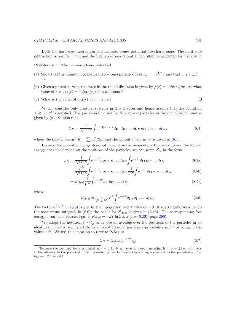
Figure 8.1: Plot of the Lennard-Jones potential uLJ(r), where r is the distance between the parti-cles. The potential is characterized by a length σ and an energy ǫ.
phenomenological form of u(r) is the Lennard-Jones or 6-12 potential shown in Figure 8.1:
uLJ(r) = 4ǫ[(σ
r
)12
−(σ
r
)6]
. (8.2)
The values of σ and ǫ for argon are σ = 3.4 × 10⁻¹⁰ m and ǫ = 1.65 × 10⁻²¹ J.
The attractive 1/r6 contribution to the Lennard-Jones potential is due to the induced dipole-dipole interaction of two neutral atoms.1 The resultant attractive interaction is called the van
der Waals potential. The rapidly increasing repulsive interaction as the separation between atomsis decreased for small r is a consequence of the Pauli exclusion principle. The 1/r12 form of therepulsive potential in (8.2) is chosen only for convenience.
The existence of many calculations and simulation results for the Lennard-Jones potentialencourages us to consider it even though there are more accurate forms of the interparticle potentialfor modeling the interactions in real fluids, proteins, and other complex molecules.
An even simpler form of the interaction between particles is the hard core interaction
uHC(r) =
{
∞ (r < σ)
0 (r > σ)(8.3)
A system of particles in three dimensions with the interaction (8.3) is called a system of hard
spheres with σ the diameter of the spheres; the analogous systems in two and one dimensions arecalled hard disks and hard rods. Although this interaction has no attractive part, we will see thatit is very useful in understanding the properties of liquids.
1A simple classical model of this induced dipole-dipole effect is described in John J. Brehm and William J.Mullin, Introduction to the Structure of Matter, John Wiley & Sons (1989), pp. 517–521.
CHAPTER 8. CLASSICAL GASES AND LIQUIDS 391
Both the hard core interaction and Lennard-Jones potential are short-range. The hard coreinteraction is zero for r > σ and the Lennard-Jones potential can often be neglected for r & 2.3 σ.2
Problem 8.1. The Lennard-Jones potential
(a) Show that the minimum of the Lennard-Jones potential is at rmin = 21/6σ and that uLJ(rmin) =−ǫ.
(b) Given a potential u(r), the force in the radial direction is given by f(r) = −du(r)/dr. At whatvalue of r is fLJ(r) = −duLJ(r)/dr a minimum?
(c) What is the value of uLJ(r) at r = 2.3 σ?
W will consider only classical systems in this chapter and hence assume that the conditionλ≪ n−1/3 is satisfied. The partition function for N identical particles in the semiclassical limit isgiven by (see Section 6.2)
ZN =1
N !h3N
∫
e−β(K+U) dp1 dp2 . . . dpN dr1 dr2 . . . drN , (8.4)
where the kinetic energy K =∑
i p2i /2m and the potential energy U is given in (8.1).
Because the potential energy does not depend on the momenta of the particles and the kineticenergy does not depend on the positions of the particles, we can write ZN in the form
ZN =1
N !h3N
∫
e−βKdp1 dp2 . . . dpN
∫
e−βUdr1 dr2 . . . drN (8.5a)
=V N
N !h3N
∫
e−βKdp1 dp2 . . . dpN1
V N
∫
e−βUdr1 dr2 . . . drN (8.5b)
= Zideal1
V N
∫
e−βUdr1dr2 . . . drN , (8.5c)
where
Zideal =1
N !h3NV N
∫
e−βKdp1 dp2 . . . dpN . (8.6)
The factor of V N in (8.6) is due to the integration over r with U = 0. It is straightforward to dothe momentum integrals in (8.6); the result for Zideal is given in (6.25). The corresponding freeenergy of an ideal classical gas is Fideal = −kT lnZideal (see (6.26), page 299).
We adopt the notation⟨
· · ·⟩
0to denote an average over the positions of the particles in an
ideal gas. That is, each particle in an ideal classical gas has a probability dr/V of being in thevolume dr. We use this notation to rewrite (8.5c) as
ZN = Zideal
⟨
e−βU⟩
0. (8.7)
2Because the Lennard-Jones potential at r = 2.3 σ is not exactly zero, truncating it at r = 2.3 σ introducesa discontinuity in the potential. This discontinuity can be avoided by adding a constant to the potential so thatuLJ = 0 at r = 2.3 σ.

CHAPTER 8. CLASSICAL GASES AND LIQUIDS 392
The contribution Fc to the free energy from the correlations between the particles due to theirinteractions has the form
Fc = F − Fideal = −kT lnZ
Zideal= −kT ln
⟨
e−βU⟩
0. (8.8)
We see that the evaluation of the free energy due to the interactions between particles can bereduced to the evaluation of the ensemble average in (8.8).
In general, we cannot calculate Fc exactly for arbitrary densities. We know that the idealgas equation of state, PV/NkT = 1, is a good approximation for a dilute gas for which theintermolecular interactions can be ignored. For this reason we first seek an approximation forFc for low densities where the interactions between the particles are not too important. If theinteractions are short-range, it is plausible that we can obtain an expansion of the pressure andhence Fc in powers of the density. This expansion is known as the density or virial expansion3 andis written as
PV
NkT= 1 + ρB2(T ) + ρ2B3(T ) + ρ3B4(T ) + . . . (8.9)
The quantities Bn are known as virial coefficients and involve the interaction of n particles. Thefirst four virial coefficients are given by the expressions (B1 = 1)
B2(T ) = − 1
2V
∫
f12 dr1dr2, (8.10a)
B3(T ) = − 1
3V
∫
f12f13f23 dr1 dr2 dr3, (8.10b)
B4(T ) = − 1
8V
∫
(
3f12f23f34f41 + 6f12f23f34f41f13
+ f12f23f34f41f13f24)
dr1dr2dr3dr4, (8.10c)
where fij = f(|ri − rj |), and
f(r) = e−βu(r) − 1 . (8.11)
The function f(r) defined in (8.11) is known as the Mayer f function.4 We will give a simplederivation of the second virial coefficient in Section 8.3. The derivation of the third and higherorder virial coefficients is much more involved and is given in Section 8.4.3.
Problem 8.2. Density expansion of the free energy
The density expansion of the free energy Fc is usually written as
− βFcN
=
∞∑
p=1
bpρp
p+ 1, (8.12)
3The word virial is related to the Latin word for force. Rudolf Clausius named a certain function of the forcebetween particles as “the virial of force.” This name was subsequently applied to the virial expansion because theterms in this expansion are related to the forces between particles.
4The f function is named after Joseph Mayer (1920–1983), a chemical physicist who is known for his work instatistical mechanics and the application of statistical mechanics to liquids and dense gases. He was the husband ofMaria Goeppert Mayer (1906–1972), who shared the Nobel Prize for physics in 1963. Maria Goeppert Mayer wasnot able to obtain a tenured faculty position until 1960 because of sexism and nepotism rules. The two of themwrote an influential text on statistical mechanics, J. E. Mayer and M. G. Mayer, Statistical Mechanics, John Wiley& Sons (1940).
CHAPTER 8. CLASSICAL GASES AND LIQUIDS 393
where the bp are known as cluster integrals. Use the thermodynamic relation P = ∂F/∂V )T,Vbetween the pressure and the free energy to show that Bn and bn−1 are related by
Bn = −n− 1
nbn−1. (8.13)
The density expansion in (8.9) and (8.12) is among the few expansions known in physics thathas a nonzero radius of convergence for a wide class of interparticle potentials. Most expansions,such as the low temperature expansion for the ideal Fermi gas, do not converge (see Section 6.11.2).
8.3 The Second Virial Coefficient
We first find the form of the second virial coefficient B2 by simple considerations. One way isto calculate the partition function for a small number of particles and to determine the effects ofincluding the interactions between particles. For N = 2 particles we have
Z2
Zideal=
1
V 2
∫
e−βu12 dr1dr2, (8.14)
where Zideal is the partition function for an ideal gas of two particles. We can simplify the integralsin (8.14) by choosing particle 1 as the origin and specifying the position of particle 2 relative toparticle 1.5 This choice of coordinates gives a factor of V because particle 1 can be anywhere inthe box. Hence, we can write (8.14) as
Z2
Zideal=
1
V
∫
e−βu(r)dr, (8.15)
where r = r2 − r1 and r = |r|.Because we wish to describe a dilute gas, we might consider writing e−βu ≈ 1 − βu, thinking
that u is small because the particles rarely interact. However, because u(r) ≫ 1 for sufficientlysmall r, the integral
∫
u(r)dr diverges. That is, the particles rarely interact, but if they do, theyinteract strongly.
Another difficulty is that the function e−βu(r) in the integrand for Z2 has the undesirableproperty that it approaches one rather than zero as r → ∞. Because we want to obtain anexpansion in the density, we want to write the integrand in (8.15) in terms of a function of r thatis significant only if two particles are close to each other. Such a function is the Mayer functionf(r) defined in (8.11). Hence we write e−βu(r) = 1 + f(r) and express (8.15) as
Z2
Zideal=
1
V
∫
[
1 + f(r)]
dr. (8.16)
In Problem 8.3 we show that f(r) → 0 for sufficiently large r for short-range potentials.
5This choice is equivalent to defining the coordinate system R = (r1 + r2)/2 and r = r2 − r1 and replacingdr1 dr2 by dR dr. Because the integrand is independent of R, we can do the integral over R and obtain a factor ofV .
CHAPTER 8. CLASSICAL GASES AND LIQUIDS 394
The first term in the integrand in (8.16) corresponds to no interactions and the second termcorresponds to the second virial coefficient B2 defined in (8.10a). To see this correspondence wechoose particle 1 as the origin as before, and rewrite (8.10a) for B2 as
B2 = −1
2
∫
f(r) dr. (8.17)
If we compare the form (8.16) and (8.17), we see that we can express Z2/Zideal in terms of B2:
Z2
Zideal= 1 − 2
VB2. (8.18)
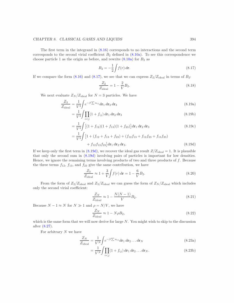
We next evaluate ZN/Zideal for N = 3 particles. We have
Z3
Zideal=
1
V 3
∫
e−βP
uijdr1 dr2 dr3 (8.19a)
=1
V 3
∫
∏
i<j
(1 + fij) dr1 dr2 dr3 (8.19b)
=1
V 3
∫
[
(1 + f12)(1 + f13)(1 + f23)]
dr1 dr2 dr3 (8.19c)
=1
V 3
∫
[
1 + (f12 + f13 + f23) + (f12f13 + f12f23 + f13f23)
+ f12f13f23]
dr1 dr2 dr3. (8.19d)
If we keep only the first term in (8.19d), we recover the ideal gas result Z/Zideal = 1. It is plausiblethat only the second sum in (8.19d) involving pairs of particles is important for low densities.Hence, we ignore the remaining terms involving products of two and three products of f . Becausethe three terms f12, f13, and f23 give the same contribution, we have
Z3
Zideal≈ 1 +
3
V
∫
f(r) dr = 1 − 6
VB2. (8.20)
From the form of Z2/Zideal and Z3/Zideal we can guess the form of ZN/Zideal which includesonly the second virial coefficient:
ZNZideal
≈ 1 − N(N − 1)
VB2. (8.21)
Because N − 1 ≈ N for N ≫ 1 and ρ = N/V , we have
ZNZideal
≈ 1 −NρB2, (8.22)
which is the same form that we will now derive for largeN . You might wish to skip to the discussionafter (8.27).
For arbitrary N we have
ZNZideal
=1
V N
∫
e−βP
uijdr1 dr2 . . . drN (8.23a)
=1
V N
∫
∏
i<j
(1 + fij) dr1 dr2 . . . drN . (8.23b)

CHAPTER 8. CLASSICAL GASES AND LIQUIDS 395
We write∏
i<j
(1 + fij) = 1 +∑
k<l
fkl +∑
k<l, m<n
fklfmn + . . . (8.24)
We keep only the ideal gas contribution and the terms involving pairs of particles and ignore theremaining terms involving products of two or more f ’s. There are a total of 1
2N(N − 1) terms inthe sum
∑
fkl corresponding to the number of ways of choosing pairs of particles. These termsare all equal because they differ only in the way the variables of integration are labeled. Hence,we can express the integral of the second sum in (8.24) as
1
V N
∫
∑
k<l
fkl dr1 . . . drN =1
V NN(N − 1)
2
∫
f(r12) dr1 . . . drN . (8.25)
The integration with respect to r3 . . . rN over the volume of the system gives a factor of V N−2.
As before, we can simplify the remaining integration over r1 and r2 by choosing particle 1as the origin and specifying particle 2 relative to particle 1. In this way we obtain an additionalfactor of V . Hence, we can write the right-hand side of (8.25) as
N(N − 1)
2
V N−2V
V N
∫
f(r) dr → N2
2V
∫
f(r) dr, (8.26)
where we have again replaced N − 1 by N . We identify the integral in (8.26) with B2 and write
ZNZideal
≈ 1 −NρB2, (8.27)
as in (8.22).
If the interparticle potential u(r) ≈ 0 for r > r0, then f(r) differs from zero only for r < r0and the integral B2 is bounded and is order r0
3 in three dimensions (see Problem 8.4). Hence B2
is independent of V and is an intensive quantity. This well-behaved nature of B2 implies that thesecond term in (8.27) is proportional to N and in the limit N → ∞ (for fixed density), this termis larger than the first – not a good start for a perturbation theory.
The reason we have obtained an apparent divergence in the density expansion of ZN/Zideal isthat we have calculated the wrong quantity. The quantity of physical interest is the free energy For lnZ, not the partition function Z. Because F is an extensive quantity and is proportional to N ,it follows from the relation F = −kT lnZ that ZN must depend on the Nth power of an intensivequantity. Hence, we expect the form of the density expansion of ZN/Zideal to be
ZNZideal
=(
1 + a1ρ+ a2ρ2 + . . .
)N, (8.28)
where an are unknown coefficients. Hence we should rewrite (8.27)
ZNZideal
≈ 1 −NρB2 ≈ (1 − ρB2)N , (8.29)
so that F is proportional to N and the correct first-order dependence on ρ is obtained. The freeenergy is given by
F = Fideal −NkT ln(1 − ρB2) ≈ Fideal +NkTρB2, (8.30)

CHAPTER 8. CLASSICAL GASES AND LIQUIDS 396
where we have used the fact that ln(1 + x) ≈ x for x≪ 1. The corresponding equation of state isgiven by
PV
NkT= 1 + ρB2, (8.31)
where we have used the relation P = −(∂F/∂V )T,N .
The second term in (8.31) represents the first-order density correction to the ideal gas equationof state. Because B2 is order r30 , the density expansion for a dilute gas is actually an expansion inpowers of the dimensionless quantity ρr30 (see Problem 8.5).
Problem 8.3. Qualitative behavior of the Mayer function
Plot the Mayer function f(r) for the hard core interaction (8.3) and the Lennard-Jones potential(8.2). Does f(r) depend on T for hard spheres? What is the qualitative behavior of f(r) for larger?
Problem 8.4. Second virial coefficient for hard spheres
(a) To calculate B2 in three dimensions we need to perform the angular integrations in (8.17).Show that because u(r) depends only on r, B2 can be written as
B2(T ) = −1
2
∫
f(r) d3r = 2π
∫ ∞
0
[
1 − e−βu(r)]
r2dr. (8.32)
(b) Show that B2 = 2πσ3/3 for a system of hard spheres of diameter σ.
(c) Determine the form of B2 for a system of hard disks.
Problem 8.5. Qualitative temperature behavior of B2(T )
Suppose that u(r) has the qualitative behavior shown in Figure 8.1; that is, u(r) is repulsive forsmall r and weakly attractive for large r. Let r0 equal the value of r at which u(r) is a minimum(see Problem 8.1) and ǫ equal the value of u at its minimum. We can write (8.32) as
B2(T ) = 2π
∫ r0
0
[
1 − e−βu(r)]
r2dr + 2π
∫ ∞
r0
[
1 − e−βu(r)]
r2dr. (8.33)
(a) For high temperatures, kT ≫ ǫ, we have u(r)/kT ≪ 1 for r > r0. Explain why the secondintegral in (8.33) can be neglected in this limit (assuming that the integral
∫ ∞
r0u(r)r2dr con-
verges) and why the dominant contribution to B2 is determined by the first integral, for whichthe integrand is approximately one because u(r)/kT is large and positive for r < r0. Hencefor high temperatures show that B2(T ) ≈ b, where
b = 2πr30/3. (8.34)
We can interpret r0 as a measure of the effective diameter of the atoms. How is the parameterb related to the “volume” of a particle?
CHAPTER 8. CLASSICAL GASES AND LIQUIDS 397
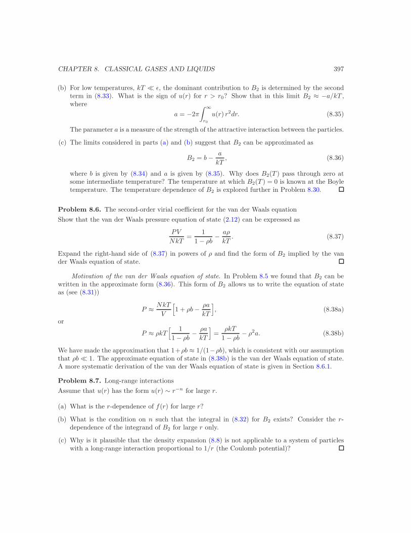
(b) For low temperatures, kT ≪ ǫ, the dominant contribution to B2 is determined by the secondterm in (8.33). What is the sign of u(r) for r > r0? Show that in this limit B2 ≈ −a/kT ,where
a = −2π
∫ ∞
r0
u(r) r2dr. (8.35)
The parameter a is a measure of the strength of the attractive interaction between the particles.
(c) The limits considered in parts (a) and (b) suggest that B2 can be approximated as
B2 = b− a
kT, (8.36)
where b is given by (8.34) and a is given by (8.35). Why does B2(T ) pass through zero atsome intermediate temperature? The temperature at which B2(T ) = 0 is known at the Boyletemperature. The temperature dependence of B2 is explored further in Problem 8.30.
Problem 8.6. The second-order virial coefficient for the van der Waals equation
Show that the van der Waals pressure equation of state (2.12) can be expressed as
PV
NkT=
1
1 − ρb− aρ
kT. (8.37)
Expand the right-hand side of (8.37) in powers of ρ and find the form of B2 implied by the vander Waals equation of state.
Motivation of the van der Waals equation of state. In Problem 8.5 we found that B2 can bewritten in the approximate form (8.36). This form of B2 allows us to write the equation of stateas (see (8.31))
P ≈ NkT
V
[
1 + ρb− ρa
kT
]
, (8.38a)
or
P ≈ ρkT[ 1
1 − ρb− ρa
kT
]
=ρkT
1 − ρb− ρ2a. (8.38b)
We have made the approximation that 1+ρb ≈ 1/(1−ρb), which is consistent with our assumptionthat ρb≪ 1. The approximate equation of state in (8.38b) is the van der Waals equation of state.A more systematic derivation of the van der Waals equation of state is given in Section 8.6.1.
Problem 8.7. Long-range interactions
Assume that u(r) has the form u(r) ∼ r−n for large r.
(a) What is the r-dependence of f(r) for large r?
(b) What is the condition on n such that the integral in (8.32) for B2 exists? Consider the r-dependence of the integrand of B2 for large r only.
(c) Why is it plausible that the density expansion (8.8) is not applicable to a system of particleswith a long-range interaction proportional to 1/r (the Coulomb potential)?

CHAPTER 8. CLASSICAL GASES AND LIQUIDS 398
8.4 *Diagrammatic Expansions
In Section 8.3 we found that we had to make some ad hoc assumptions to obtain the form ofB2 from an expansion of Z/Zideal. To find the form of the higher order virial coefficients moresystematically, we will introduce a formalism that allows us to obtain a density expansion of thefree energy directly rather than first approximating the partition function. In Section 8.4.2 we firstobtain the expansion of the free energy in powers of the inverse temperature β. We will find thatit is convenient to represent the contributions to the free energy due to the interactions betweenparticles in terms of diagrams. We rearrange this expansion in Section 8.4.3 so that it becomes anexpansion in powers of the density ρ.
8.4.1 *Cumulants
The form (8.8) for Fc is similar to that frequently encountered in probability theory (see Sec-tion 3.11.2, page 157). We define the function φ(t) as
φ(t) ≡⟨
etx⟩
, (8.39)
where the random variable x occurs according to the probability distribution p(x), that is, theaverage denoted by
⟨
. . .⟩
is over p(x). The function φ(t) is an example of a moment generating
function because a power series expansion in t yields
φ(t) =⟨[
1 + tx+1
2!t2x2 + · · ·
]⟩
(8.40a)
= 1 + t⟨
x⟩
+t2
2!
⟨
x2⟩
+ · · · (8.40b)
=
∞∑
n=0
tn⟨
xn⟩
n!. (8.40c)
In the present case the quantity of interest is proportional to lnZ, so we want to consider theseries expansion of lnφ rather than φ. (The correspondence is t → −β and x → U .) The seriesexpansion of lnφ(t) can be written in the form
lnφ = ln⟨
etx⟩
=
∞∑
n=1
tnMn(x)
n!, (8.41)
where the coefficients Mn are known as cumulants. The first four cumulants are
M1 =⟨
x⟩
, (8.42a)
M2 =⟨
x2⟩
−⟨
x⟩2, (8.42b)
M3 =⟨
x3⟩
− 3⟨
x2⟩⟨
x⟩
+ 2⟨
x⟩3, (8.42c)
M4 =⟨
x4⟩
− 4⟨
x3⟩⟨
x⟩
− 3⟨
x2⟩2
+ 12⟨
x2⟩⟨
x⟩2 − 6
⟨
x⟩4. (8.42d)
CHAPTER 8. CLASSICAL GASES AND LIQUIDS 399
Problem 8.8. The first four cumulants
Expand ln(1+x) in a Taylor series (see (A.4)) and obtain the expressions forMn given in (8.42).
The advantage of working with cumulants can be seen by considering two independent randomvariables, x and y. Because x and y are statistically independent, we have
⟨
xy⟩
=⟨
x⟩⟨
y⟩
, and
ln⟨
et(x+y)⟩
= ln⟨
etx⟩⟨
ety⟩
= ln⟨
etx⟩
+ ln⟨
ety⟩
. (8.43)
From the relation
ln⟨
et(x+y)⟩
=
∞∑
n=0
tn
n!Mn(x+ y), (8.44)
we see that Mn satisfies the additive property:
Mn(x+ y) = Mn(x) +Mn(y). (8.45)
The relation (8.45) implies that all cross terms in Mn involving independent variables vanish, andhence lnφ(x) is an extensive or additive quantity.
Example 8.1. Cancellation of cross terms in M2
Show that the cross terms cancel in M2.
Solution. We have
M2(x+ y) =⟨
(x+ y)2⟩
−⟨
(x+ y)⟩2
(8.46a)
=⟨
x2⟩
+�
��
�2⟨
x⟩⟨
y⟩
+⟨
y2⟩
−⟨
x⟩2 −
��
��2
⟨
x⟩⟨
y⟩
+⟨
y⟩2
(8.46b)
=⟨
x2⟩
−⟨
x⟩2
+⟨
y2⟩
−⟨
y⟩2
(8.46c)
= M2(x) +M2(y). (8.46d)
♦
Problem 8.9. Cancellation of cross terms in M3
As an example of the cancellation of cross terms, consider M3(x + y). From (8.42c) we see thatM3(x+ y) is given by
M3(x+ y) = (x + y)3 − 3(x+ y)2 (x+ y) + 2(x+ y)3
(8.47)
Show explicitly that all cross terms cancel and hence that M3(x + y) = M3(x) +M3(y).
8.4.2 *High temperature expansion
Now that we have discussed the formal properties of the cumulants, we can use these propertiesto evaluate Fc. According to (8.8) and (8.41) we can write Fc as
− βFc = ln⟨
e−βU⟩
0=
∞∑
n=1
(−β)n
n!Mn. (8.48)

CHAPTER 8. CLASSICAL GASES AND LIQUIDS 400
The expansion (8.48) in powers of β is known as a high temperature expansion. Such an expansion isnatural because β is the only parameter that appears explicitly in (8.48). The parameter β actuallyappears in the dimensionless combination βu0, where the energy u0 is a measure of the strength ofthe interaction. Although we can choose β to be as small as we wish, the interparticle interactionfor potentials such as the Lennard-Jones potential is strongly repulsive at short distances (seeFigure 8.1), and hence ǫ is not well defined. For this reason a strategy based on expanding in theparameter β is not physically reasonable for an interaction such as the Lennard-Jones potential.
Because of these difficulties, we will first do what we can and then do what we want. Thus wewill first determine the high temperature expansion coefficients Mn and assume that the potentialis not strongly repulsive for small r. For example, we can choose u(r) to have the form u(r) =
u0e−r2/a2
for small r. Then we will find that we can reorder the high temperature expansion toobtain a power series expansion in the density. Because it will be easy to become lost in the details,we emphasize that the main points of this section are the association of diagrams with the variouscontributions to the cumulants and the fact that only certain kinds of diagrams actually contributeto the free energy.
The first cumulant in the expansion (8.48) is the average of the total potential energy:
M1 =⟨
U⟩
=1
V N
∫
∑
i<j
uij dr1 dr2 . . . drN . (8.49)
Because every term in the sum gives the same contribution, we have
M1 =1
2N(N − 1)
1
V N
∫
u12 dr1 dr2 . . . drN (8.50a)
=1
2N(N − 1)
1
V NV N−2
∫
u12 dr1 dr2 (8.50b)
=1
2N(N − 1)
1
V 2
∫
u12 dr1 dr2. (8.50c)
The combinatorial factor 12N(N −1) is the number of terms in the sum. Because we are interested
in the limit N → ∞, we replace N − 1 by N . We can simplify (8.50c) further by measuring theposition of particle 2 from particle 1. We obtain
M1 =N2
2V 2V
∫
u(r) dr, (8.51a)
or
M1 =ρ
2N
∫
u(r) dr. (8.51b)
Note that M1 is an extensive quantity as is the free energy; that is, M1 is proportional to N . Notethat the integral in (8.51b) diverges for small r for the Lennard-Jones potential (8.2) and the hardcore interaction (8.3), but converges for a Gaussian potential.
We next consider M2 which is given by
M2 =⟨
U2⟩
−⟨
U⟩2, (8.52)
where
CHAPTER 8. CLASSICAL GASES AND LIQUIDS 401
⟨
U⟩
=∑
i<j
∑
j
⟨
uij⟩
, (8.53)
and⟨
U2⟩
=∑
i<j
∑
j
∑
k<l
∑
l
⟨
uij ukl⟩
, (8.54)
The various terms in (8.54) and (8.53) may be classified according to the number of subscripts incommon. As an example, consider a system of N = 4 particles. We have
U =N=4∑
i<j=1
uij = u12 + u13 + u14 + u23 + u24 + u34, (8.55)
and
U2 =[
u212 + u2
13 + u214 + u2
23 + u224 + u2
34]
+ 2[u12u13 + u12u14 + u12u23 + u12u24 + u13u14 + u13u23
+ u13u34 + u14u24 + u14u34 + u23u24 + u23u34 + u24u34]
+ 2[u12u34 + u13u24 + u14u23
]
. (8.56)
An inspection of (8.56) shows that the 36 terms in (8.56) can be grouped into three classes:
No indices in common (disconnected terms). A typical disconnected term is⟨
u12u34
⟩
.Because the variables r12 and r34 are independent, u12 and u34 are independent, and we can write
⟨
u12u34
⟩
=⟨
u12
⟩⟨
u34
⟩
. (8.57)
From (8.45) we know that every disconnected term such as the one in (8.57) is a cross term thatis canceled if all terms in M2 are included.
One index in common (reducible terms). An example of a reducible term is⟨
u12u23
⟩
.Such a term also factorizes because of the homogeneity of space. We choose particle 2 as the originand integrate over r1 and r3 and find
⟨
u12u23
⟩
=1
V 3
∫
u12 u23 dr1 dr2 dr3 (8.58a)
=1
V 2
∫
u12 u23 dr12 dr23 (8.58b)
=⟨
u12
⟩⟨
u23
⟩
. (8.58c)
A factor of V was obtained because particle 2 can be anywhere in the box of volume V . Again wefind that the variables u12u23 are independent and hence are canceled by other terms in M2.
Both pairs of indices in common (irreducible terms). An example of an irreducibleterm is
⟨
u212
⟩
. The corresponding contribution to M2 is (see (8.52))
M2 =
N∑
i<j=1
[⟨
u2ij
⟩
−⟨
uij⟩2]
. (8.59)

CHAPTER 8. CLASSICAL GASES AND LIQUIDS 402
We can simplify (8.59) by comparing the magnitude of the two types of terms in the limit N → ∞.We have that
⟨
u2ij
⟩
=1
V
∫
u2ij drij ∝
1
V∝ O
( 1
N
)
. (8.60a)
⟨
uij⟩2
=( 1
V
∫
uij drij
)2
∝ O( 1
N2
)
. (8.60b)
We see that we can ignore the second term in comparison to the first.
These considerations lead us to the desired form ofM2. Because there areN(N−1)/2 identicalcontributions such as (8.60a) to M2 in (8.59), we obtain
M2 =N(N − 1)
2V
∫
u2(r) dr → ρ
2N
∫
u2(r) dr. (8.61)
The most important result of our evaluation of M1 and M2 is that the disconnected andreducible contributions do not contribute. The vanishing of the disconnected contributions isessential for Mn and thus for Fc to be an extensive quantity. For example, consider the contribution∑
i<j,k<l
⟨
uij⟩⟨
ukl⟩
for i 6= j 6= k 6= l. As we saw in (8.60b), each⟨
uij⟩
is order 1/V . Because
each index is different, the number of terms is ∼ N4 and hence the order of magnitude of thistype of contribution is N4/V 2 ∼ N2. (Recall that N/V = ρ is finite.) Because the presence of thedisconnected terms in M2 would imply that Fc would be proportional to N2 rather than N , it isnecessary that this spurious N dependence cancel exactly. The fact that the disconnected termsdo not contribute to Fc was first shown for a classical system of particles by Joseph Mayer in 1937.The corresponding result was not established for a quantum system of particles until 1957.6
The reducible terms also vanish but do not lead to a spurious N -dependence. As an example,consider the term
⟨
uijujkukl⟩
with four distinct indices. We can choose relative coordinates and
show that⟨
uijujkukl⟩
=⟨
uij⟩⟨
ujk⟩⟨
ukl⟩
, and hence is canceled for a classical gas. The N -dependence of this term is N4/V 3 ∼ N . The reducible terms do not cancel for quantum systems.
Problem 8.10. The first two cumulants for a system of four particles
Consider a system of N = 4 particles and obtain the explicit form of M2. Show that the discon-nected and reducible contributions cancel.
To simplify the calculation of the higher order cumulants and to understand the differencebetween the disconnected, reducible and irreducible terms, it is convenient to introduce a graphicalnotation that corresponds to the various contributions to Mn. As we have seen, we do not need toconsider products of expectation values because they either cancel or are O(1/N) relative to theirreducible terms arising from the first term in Mn. The rules for the calculation of Mn can bestated in graphical terms as follows:
(1) For each particle (subscript on u) draw a vertex (a point).
6K. A. Brueckner, “Many-body problem for strongly interacting particles. II. Linked cluster expansion,” Phys.Rev. 100, 36–45 (1955) J. Goldstone, “Derivation of Brueckner many-body theory,” Proc. Roy. Soc. A 239, 267–279 (1957). The latter paper uses Feynman diagrams. A more accessible introduction to Feynman diagrams isby Richard D. Mattuck, A Guide to Feynman Diagrams in the Many-Body Problem, second edition, Dover Books(1992).
CHAPTER 8. CLASSICAL GASES AND LIQUIDS 403
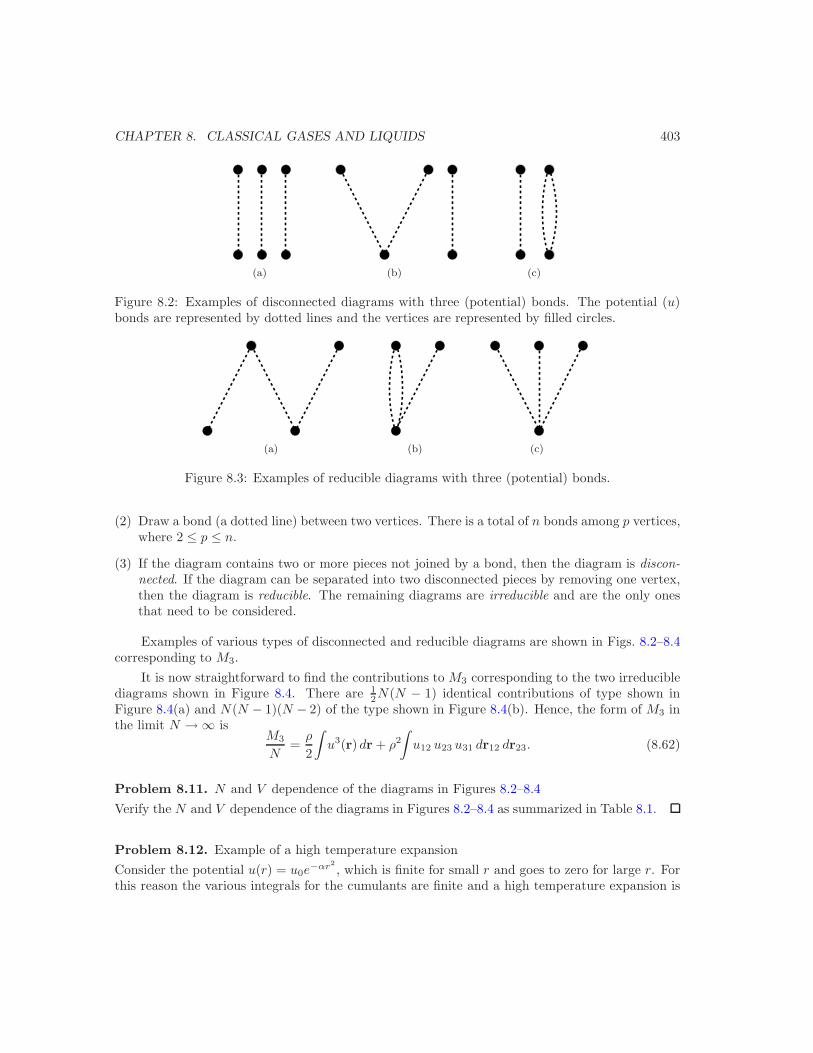
(a) (b) (c)
Figure 8.2: Examples of disconnected diagrams with three (potential) bonds. The potential (u)bonds are represented by dotted lines and the vertices are represented by filled circles.
(a) (b) (c)
Figure 8.3: Examples of reducible diagrams with three (potential) bonds.
(2) Draw a bond (a dotted line) between two vertices. There is a total of n bonds among p vertices,where 2 ≤ p ≤ n.
(3) If the diagram contains two or more pieces not joined by a bond, then the diagram is discon-
nected. If the diagram can be separated into two disconnected pieces by removing one vertex,then the diagram is reducible. The remaining diagrams are irreducible and are the only onesthat need to be considered.
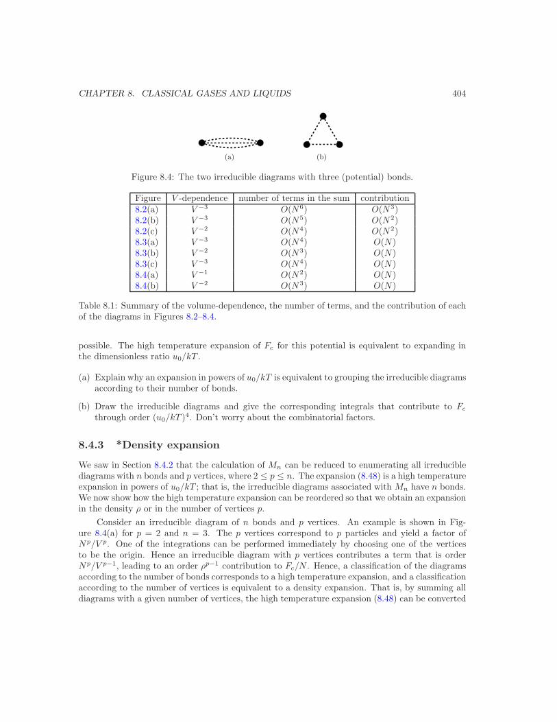
Examples of various types of disconnected and reducible diagrams are shown in Figs. 8.2–8.4corresponding to M3.
It is now straightforward to find the contributions to M3 corresponding to the two irreduciblediagrams shown in Figure 8.4. There are 1
2N(N − 1) identical contributions of type shown inFigure 8.4(a) and N(N − 1)(N − 2) of the type shown in Figure 8.4(b). Hence, the form of M3 inthe limit N → ∞ is
M3
N=ρ
2
∫
u3(r) dr + ρ2
∫
u12 u23 u31 dr12 dr23. (8.62)
Problem 8.11. N and V dependence of the diagrams in Figures 8.2–8.4
Verify the N and V dependence of the diagrams in Figures 8.2–8.4 as summarized in Table 8.1.
Problem 8.12. Example of a high temperature expansion
Consider the potential u(r) = u0e−αr2 , which is finite for small r and goes to zero for large r. For
this reason the various integrals for the cumulants are finite and a high temperature expansion is
CHAPTER 8. CLASSICAL GASES AND LIQUIDS 404
(a) (b)
Figure 8.4: The two irreducible diagrams with three (potential) bonds.
Figure V -dependence number of terms in the sum contribution8.2(a) V −3 O(N6) O(N3)8.2(b) V −3 O(N5) O(N2)8.2(c) V −2 O(N4) O(N2)8.3(a) V −3 O(N4) O(N)8.3(b) V −2 O(N3) O(N)8.3(c) V −3 O(N4) O(N)8.4(a) V −1 O(N2) O(N)8.4(b) V −2 O(N3) O(N)
Table 8.1: Summary of the volume-dependence, the number of terms, and the contribution of eachof the diagrams in Figures 8.2–8.4.
possible. The high temperature expansion of Fc for this potential is equivalent to expanding inthe dimensionless ratio u0/kT .
(a) Explain why an expansion in powers of u0/kT is equivalent to grouping the irreducible diagramsaccording to their number of bonds.
(b) Draw the irreducible diagrams and give the corresponding integrals that contribute to Fcthrough order (u0/kT )4. Don’t worry about the combinatorial factors.
8.4.3 *Density expansion
We saw in Section 8.4.2 that the calculation of Mn can be reduced to enumerating all irreduciblediagrams with n bonds and p vertices, where 2 ≤ p ≤ n. The expansion (8.48) is a high temperatureexpansion in powers of u0/kT ; that is, the irreducible diagrams associated with Mn have n bonds.We now show how the high temperature expansion can be reordered so that we obtain an expansionin the density ρ or in the number of vertices p.
Consider an irreducible diagram of n bonds and p vertices. An example is shown in Fig-ure 8.4(a) for p = 2 and n = 3. The p vertices correspond to p particles and yield a factor ofNp/V p. One of the integrations can be performed immediately by choosing one of the verticesto be the origin. Hence an irreducible diagram with p vertices contributes a term that is orderNp/V p−1, leading to an order ρp−1 contribution to Fc/N . Hence, a classification of the diagramsaccording to the number of bonds corresponds to a high temperature expansion, and a classificationaccording to the number of vertices is equivalent to a density expansion. That is, by summing alldiagrams with a given number of vertices, the high temperature expansion (8.48) can be converted

CHAPTER 8. CLASSICAL GASES AND LIQUIDS 405
(a) (b)
Figure 8.5: (a) The first several irreducible diagrams with two vertices and n = 1, 2, and 3 potentialbonds (dotted lines). (b) The equivalent diagram with one Mayer f bond (solid line).
to an expansion in the density. The result is traditionally written in the form (see (8.12))
− βFcN
=
∞∑
p=1
bp ρp
p+ 1. (8.63)
In the following we will find the form of the first few cluster integrals bp.
We first add the contribution of all the two-vertex diagrams to find b1 (see Figure 8.5(a)).From (8.48) we see that a factor of −β is associated with each bond. The contribution to −βFcfrom all two vertex irreducible diagrams is
∞∑
n=1
(−β)n
n!Mn = N
ρ
2
∞∑
n=1
(−β)n
n!
∫
un(r) dr = Nρ
2
∫
(e−βu(r) − 1) dr. (8.64)
Because B2 = − 12b1 (see (8.13), we recover the result (8.32) that we found in Section 8.2 by a
plausibility argument. Note the appearance of the Mayer f function in (8.64) and that f emergesby summing an infinite number of potential bonds between two particles.
We can now simplify the diagrammatic expansion by replacing the infinite sum of u (potential)bonds between any two particles by f . For example, b1 corresponds to the single diagram shownin Figure 8.5(b), where the solid line represents the Mayer f function.
To find b2 we consider the set of all irreducible diagrams with n = 3 vertices. Some of thediagrams with u bonds are shown in Figure 8.6(a). By considering all the possible combinationsof the u bonds, we can sum up all the irreducible diagrams with three vertices with l12, l23, andl31 bonds. Instead, we will use our intuition and replace the various combinations of u bondsbetween two vertices by a single f bond between any two vertices as shown in Figure 8.6(b). Thecorresponding contribution to b2 is
b2 =1
2!
∫
f12f23f31 dr12 dr23. (8.65)
It can be shown that bp is the sum over all topologically distinct irreducible diagrams amongp+ 1 vertices. For example, b3 corresponds to the four-vertex diagrams shown in Figure 8.7. Thecorresponding result for b3 is
b3 =1
3!
∫
(3f12f23f34f41 + 6f12f23f34f41f13 + f12f23f34f41f13f24) dr2 dr3 dr4. (8.66)

CHAPTER 8. CLASSICAL GASES AND LIQUIDS 406
(a) (b)
Figure 8.6: (a) The first several irreducible diagrams with three vertices and various numbers of ubonds (dotted lines). (b) The corresponding diagram with f -bonds (solid lines).
3
1 2
4
2
1 4
3
3
1 4
2
3
1 2
4
2
1 4
3
3
1 4
2
3
1 2
4
2
1 4
3
3
1 4
2
3
1 2
4
Figure 8.7: The four-vertex diagrams with all the possible different labelings. Note that the bondsare f bonds.
We see that we have converted the original high temperature expansion to a density expan-sion for the free energy and by summing what are known as ladder diagrams. These diagramscorresponding to all the possible u bonds between any two particles (vertices). The result of thissum is the Mayer f function.
The procedure for finding higher order terms in the density expansion of the free energy isstraightforward in principle. To find the contribution of order ρp−1 we enumerate all the irreduciblediagrams with p vertices and various numbers of f bonds. There is only one f bond between anytwo vertices. The enumeration of the cluster integrals bp becomes more and more tedious for largerp, and it becomes increasingly difficult to determine the combinatorial factors such as the factorsof 3, 6, and 1 in (8.66).
8.4.4 Higher order virial coefficients for hard spheres
The values of the first six virial coefficients (not counting B1 = 1) for hard spheres are given inTable 8.2 in terms of the dimensionless parameter
η = πρσ3/6, (8.67)
where σ is the diameter of the spheres. The parameter η can be expressed as
η =N
4π
3
(σ
2
)3
V= ρ
4π
3
(σ
2
)3
. (8.68)
The form of (8.68) shows that η is the fraction of the space occupied by N spheres. For this reason ηis called the packing fraction. The second virial coefficientB2 was calculated in Problem 8.4 for hard
CHAPTER 8. CLASSICAL GASES AND LIQUIDS 407
virial coefficient magnitude
ρB223πρσ
3 = 4ηρ2B3
518π
2ρ2σ6 = 10η2
ρ3B4 18.365η3
ρ4B5 28.24η4
ρ5B6 39.5η5
ρ6B7 56.5η6
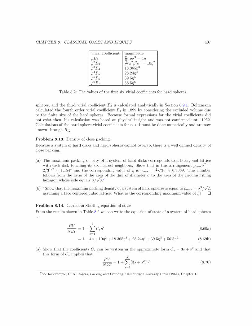
Table 8.2: The values of the first six virial coefficients for hard spheres.
spheres, and the third virial coefficient B3 is calculated analytically in Section 8.9.1. Boltzmanncalculated the fourth order virial coefficient B4 in 1899 by considering the excluded volume dueto the finite size of the hard spheres. Because formal expressions for the virial coefficients didnot exist then, his calculation was based on physical insight and was not confirmed until 1952.Calculations of the hard sphere virial coefficients for n > 4 must be done numerically and are nowknown through B12.
Problem 8.13. Density of close packing
Because a system of hard disks and hard spheres cannot overlap, there is a well defined density ofclose packing.
(a) The maximum packing density of a system of hard disks corresponds to a hexagonal latticewith each disk touching its six nearest neighbors. Show that in this arrangement ρmaxσ
2 =2/31/2 ≈ 1.1547 and the corresponding value of η is ηmax = 1
6
√3π ≈ 0.9069. This number
follows from the ratio of the area of the disc of diameter σ to the area of the circumscribinghexagon whose side equals σ/
√3.7
(b) *Show that the maximum packing density of a system of hard spheres is equal to ρmax = σ3/√
2,assuming a face centered cubic lattice. What is the corresponding maximum value of η?
Problem 8.14. Carnahan-Starling equation of state
From the results shown in Table 8.2 we can write the equation of state of a system of hard spheresas
PV
NkT= 1 +
6∑
s=1
Csηs (8.69a)
= 1 + 4η + 10η2 + 18.365η3 + 28.24η4 + 39.5η5 + 56.5η6. (8.69b)
(a) Show that the coefficients Cs can be written in the approximate form Cs = 3s+ s2 and thatthis form of Cs implies that
PV
NkT= 1 +
∞∑
s=1
(3s+ s2)ηs. (8.70)
7See for example, C. A. Rogers, Packing and Covering, Cambridge University Press (1964), Chapter 1.

CHAPTER 8. CLASSICAL GASES AND LIQUIDS 408
(b) Do the sum in (8.70) and show that
PV
NkT=
1 + η + η2 − η3
(1 − η)3. (8.71)
(Hint: start with the infinite sum∑∞s=0 η
s = (1− η)−1 and take derivatives of both sides withrespect to η.) The form (8.71) is known as the Carnahan-Starling equation of state and is agood approximation to the equation of state found by Monte Carlo simulations.
(c) Use the Carnahan-Starling equation of state (8.71) to derive analytical expressions for theentropy S, energy E, and the Helmholtz free energy F for a hard sphere fluid.
The virial coefficients for a gas of particles interacting via the Lennard-Jones potential can bedone numerically (see Problem 8.30 for a calculation of B2).
8.5 The Radial Distribution Function
Now that we know how to include the interactions between particles to obtain the equation ofstate of a dilute gas, we consider how these interactions lead to correlations between the particles.We know that if the interactions are neglected, the positions of the particles are uncorrelated, andthe probability of finding a particle a distance r away from a particular particle is proportional tothe density ρ. In the following, we will introduce the radial distribution function g(r) as a measureof the correlations between particles due to their interactions. This function is analogous to thespin-spin correlation function introduced in Section 5.5.2.
Suppose that we choose the origin of our coordinate system at a particular particle (say particleone). Then the quantity ρg(r)dr is defined as the mean number of particles that are within thedistance r and r + dr from the origin. That is,
ρg(r) = mean local density a distance r from a given particle. (8.72)
If the gas is dilute, we need to consider only the effect of the interactions between particleone and any other particle and ignore the effects of all the other particles. Because the energy ofinteraction between two particles is u(r), the form of g(r) for a dilute gas is given by
g(r) = e−βu(r), (dilute gas) (8.73)
where e−βu(r) is the probability that another particle is a distance r away. We will derive the lowdensity limit (8.73) in the following. Note that if u(r) = 0, then g(r) = 1, and the mean localdensity equals the mean density ρ.
The radial distribution function g(r) is important because it can be measured experimentallyand in simulations and because the mean energy and mean pressure can be calculated from g(r).We will show that the mean energy is given by
E =3
2NkT +
ρ
2N
∫ ∞
0
u(r)g(r) 4πr2dr, (8.74)
and the mean pressure is given by
CHAPTER 8. CLASSICAL GASES AND LIQUIDS 409
r
∆r
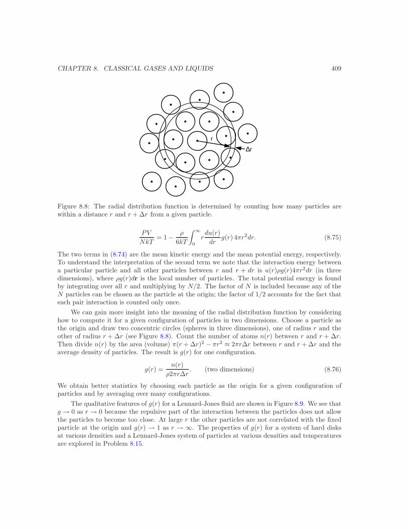
Figure 8.8: The radial distribution function is determined by counting how many particles arewithin a distance r and r + ∆r from a given particle.
PV
NkT= 1 − ρ
6kT
∫ ∞
0
rdu(r)
drg(r) 4πr2dr. (8.75)
The two terms in (8.74) are the mean kinetic energy and the mean potential energy, respectively.To understand the interpretation of the second term we note that the interaction energy betweena particular particle and all other particles between r and r + dr is u(r)ρg(r)4πr2dr (in threedimensions), where ρg(r)dr is the local number of particles. The total potential energy is foundby integrating over all r and multiplying by N/2. The factor of N is included because any of theN particles can be chosen as the particle at the origin; the factor of 1/2 accounts for the fact thateach pair interaction is counted only once.
We can gain more insight into the meaning of the radial distribution function by consideringhow to compute it for a given configuration of particles in two dimensions. Choose a particle asthe origin and draw two concentric circles (spheres in three dimensions), one of radius r and theother of radius r + ∆r (see Figure 8.8). Count the number of atoms n(r) between r and r + ∆r.Then divide n(r) by the area (volume) π(r + ∆r)2 − πr2 ≈ 2πr∆r between r and r + ∆r and theaverage density of particles. The result is g(r) for one configuration.
g(r) =n(r)
ρ2πr∆r. (two dimensions) (8.76)
We obtain better statistics by choosing each particle as the origin for a given configuration ofparticles and by averaging over many configurations.
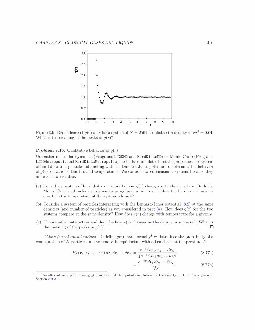
The qualitative features of g(r) for a Lennard-Jones fluid are shown in Figure 8.9. We see thatg → 0 as r → 0 because the repulsive part of the interaction between the particles does not allowthe particles to become too close. At large r the other particles are not correlated with the fixedparticle at the origin and g(r) → 1 as r → ∞. The properties of g(r) for a system of hard disksat various densities and a Lennard-Jones system of particles at various densities and temperaturesare explored in Problem 8.15.
CHAPTER 8. CLASSICAL GASES AND LIQUIDS 410
0.0
0.5
1.0
1.5
2.0
2.5
3.0
0 1 2 3 4 5 6 7 8 9 10
g(r)
r
Figure 8.9: Dependence of g(r) on r for a system of N = 256 hard disks at a density of ρσ2 = 0.64.What is the meaning of the peaks of g(r)?
Problem 8.15. Qualitative behavior of g(r)
Use either molecular dynamics (Programs LJ2DMD and HardDisksMD) or Monte Carlo (ProgramsLJ2DMetropolis and HardDisksMetropolis)methods to simulate the static properties of a systemof hard disks and particles interacting with the Lennard-Jones potential to determine the behaviorof g(r) for various densities and temperatures. We consider two-dimensional systems because theyare easier to visualize.
(a) Consider a system of hard disks and describe how g(r) changes with the density ρ. Both theMonte Carlo and molecular dynamics programs use units such that the hard core diameterσ = 1. Is the temperature of the system relevant?
(b) Consider a system of particles interacting with the Lennard-Jones potential (8.2) at the samedensities (and number of particles) as you considered in part (a). How does g(r) for the twosystems compare at the same density? How does g(r) change with temperature for a given ρ
(c) Choose either interaction and describe how g(r) changes as the density is increased. What isthe meaning of the peaks in g(r)?
∗More formal considerations. To define g(r) more formally8 we introduce the probability of aconfiguration of N particles in a volume V in equilibrium with a heat bath at temperature T :
PN (r1, r2, . . . , rN ) dr1 dr2 . . . drN =e−βUdr1dr2 . . . drN
∫
e−βUdr1 dr2 . . . drN(8.77a)
=e−βUdr1 dr2 . . . drN
QN, (8.77b)
8An alternative way of defining g(r) in terms of the spatial correlations of the density fluctuations is given inSection 8.9.2.

CHAPTER 8. CLASSICAL GASES AND LIQUIDS 411
where U is the total potential energy of the configuration. The quantity PN dr1dr2 . . . drN is theprobability that particle 1 is in the range dr1 about r1, particle 2 is in the range dr2 about r2, etc.Note that the probability density PN (r1, r2, . . . , rN ) is properly normalized.
It is convenient to define the configuration integral QN as
QN =
∫
e−βU dr1 dr2 . . . drN . (8.78)
The configuration integral QN is related to the partition function ZN by
QN = ZN/(N !λ3N ). (8.79)
QN is defined so that QN = V N for an ideal gas.
The probability that particle 1 is in the range dr1 about r1 and particle 2 is in the range dr2
about r2 is obtained by integrating (8.77) over the positions of particles 3 through N :
P2(r1, r2) dr1dr2 =
∫
e−βUdr3 . . . drNQN
dr1dr2. (8.80)
The probability that any particle is in the range dr1 about r1 and any other particle is in therange dr2 about r2 is N(N − 1)P2 dr1dr2. The pair distribution function g(r1, r2) is defined as
ρ2g(r1, r2) = N(N − 1)P2 = N(N − 1)
∫
e−βUdr3 . . . drNQN
. (8.81)
We use ρ = N/V to write g as
g(r1, r2) =(
1 − 1
N
)V 2∫
e−βUdr3 . . . drNQN
. (8.82)
If the interparticle interaction is spherically symmetric and the system is a fluid (a liquid or a gas),then g(r1, r2) depends only on the distance r = |r1 − r2| between particles 1 and 2. We adopt thenotation g(r) = g(r12) and define the radial distribution function g(r) as
g(r) =(
1 − 1
N
)V 2∫
e−βUdr3 . . . drNQN
. (8.83)
Note that (8.83) implies that g(r) = 1−1/N for an ideal gas. We can ignore the 1/N correctionin the thermodynamic limit so that g(r) = 1. From (8.83) we see that the normalization of ρg(r)is given by (for d = 3)
ρ
∫
g(r)4πr2dr = ρ(
1 − 1
N
)
V 2 1
V= N − 1 ≈ N. (8.84)
To determine g(r) for a dilute gas we write g(r) as (see (8.83))
g(r) =V 2
∫
e−βUdr3 . . . drNQN
, (8.85)

CHAPTER 8. CLASSICAL GASES AND LIQUIDS 412
where we have taken the limit N → ∞. At low densities, we can integrate over particles 3, 4,. . . , N , assuming that these particles are distant from particles 1 and 2 and also distant from eachother. Also for almost all configurations we can replace U by u12 in the numerator. Similarly, thedenominator can be approximated by V N . Hence (8.85) reduces to
g(r) ≈ V 2 e−βu12V N−2
V N= e−βu(r), (8.86)
as given in (8.73).
To obtain the relation (8.74) for the mean total energy E in terms of g(r) we write
E =3
2NkT + U, (8.87)
where
U =1
QN
∫
· · ·∫
Ue−βU dr1dr2 . . . drN . (8.88)
We assume that U is given by (8.1) and write U as
U =N(N − 1)
2
1
QN
∫
e−βUu(r12) dr1 . . . drN (8.89a)
=N(N − 1)
2
∫
u(r12)
[∫
e−βU dr3 . . . drNQN
]
dr1dr2. (8.89b)
From (8.82) we see that the term in brackets is related to ρ2g(r1, r2). Hence we we can write U as
U =1
2
∫
u(r12 ρ2g(r1, r2) dr1dr2 =
N2
2V
∫
u(r)g(r)dr (8.90a)
= Nρ
2
∫
u(r)g(r) 4πr2dr. (8.90b)
We assumed three dimensions to obtain (8.90b).
The derivation of the relation (8.75) between the mean pressure and g(r) is more involved.We write the pressure in terms of QN :
P = −∂F∂V
= kT∂ lnQN∂V
. (8.91)
Recall that QN = V N for an ideal gas. For large V the pressure is independent of the shape of thecontainer. For convenience, we assume that the container is a cube of linear dimension L, and wewrite QN as
QN =
∫ L
0
· · ·∫ L
0
e−βU dx1 dy1 dz1 . . . dxN dyN dzN . (8.92)
We first change variables so that the limits of integration are independent of L and let xi = xi/L,etc. This change of variables allows us to take the derivative of QN with respect to V . We have
QN = V N∫ 1
0
. . .
∫ 1
0
e−βUdx1 dy1 dz1 . . . dxN dyN dzN , (8.93)

CHAPTER 8. CLASSICAL GASES AND LIQUIDS 413
where U depends on the separation rij = L[(xi − xj)2 + (yi − yj)
2 + (xi − zj)2]1/2. We now take
the derivative
∂QN∂V
= NV N−1
∫ 1
0
· · ·∫ 1
0
e−βUdx1 . . . dzN
− V N
kT
∫ 1
0
· · ·∫ 1
0
e−βU∂U
∂Vdx1 . . . dzN , (8.94)
where∂U
∂V=
∑
i<j
du(rij)
drij
drijdL
dL
dV=
∑
i<j
du(rij)
drij
rijL
1
3L2. (8.95)
Now that we have differentiated QN with respect to V , we transform back to the original variablesx1, . . . , zN . In the second term of (8.95) we also use the fact that there are N(N − 1)/2 identicalcontributions. In this way we obtain
∂ lnQN∂V
=1
QN
∂QN∂V
=N
V− ρ2
6V kT
∫
r12du(r12)
dr12g(r12) dr1 dr2, (8.96)
and hence
PV
NkT= 1 − ρ
6kT
∫ ∞
0
rdu(r)
drg(r) 4πr2dr. (virial equation of state) (8.97)
The integrand in (8.97) is related to the virial in classical mechanics and is the mean value of theproduct r · F (cf. Goldstein).
∗Density expansion of g(r). The density expansion of g(r) is closely related to the densityexpansion of the free energy. Instead of deriving the relation here, we show only the diagramscorresponding to the first two density contributions. We write
g(r) = e−βu(r)y(r), (8.98)
and
y(r) =∞∑
n=0
ρnyn(r), (8.99)
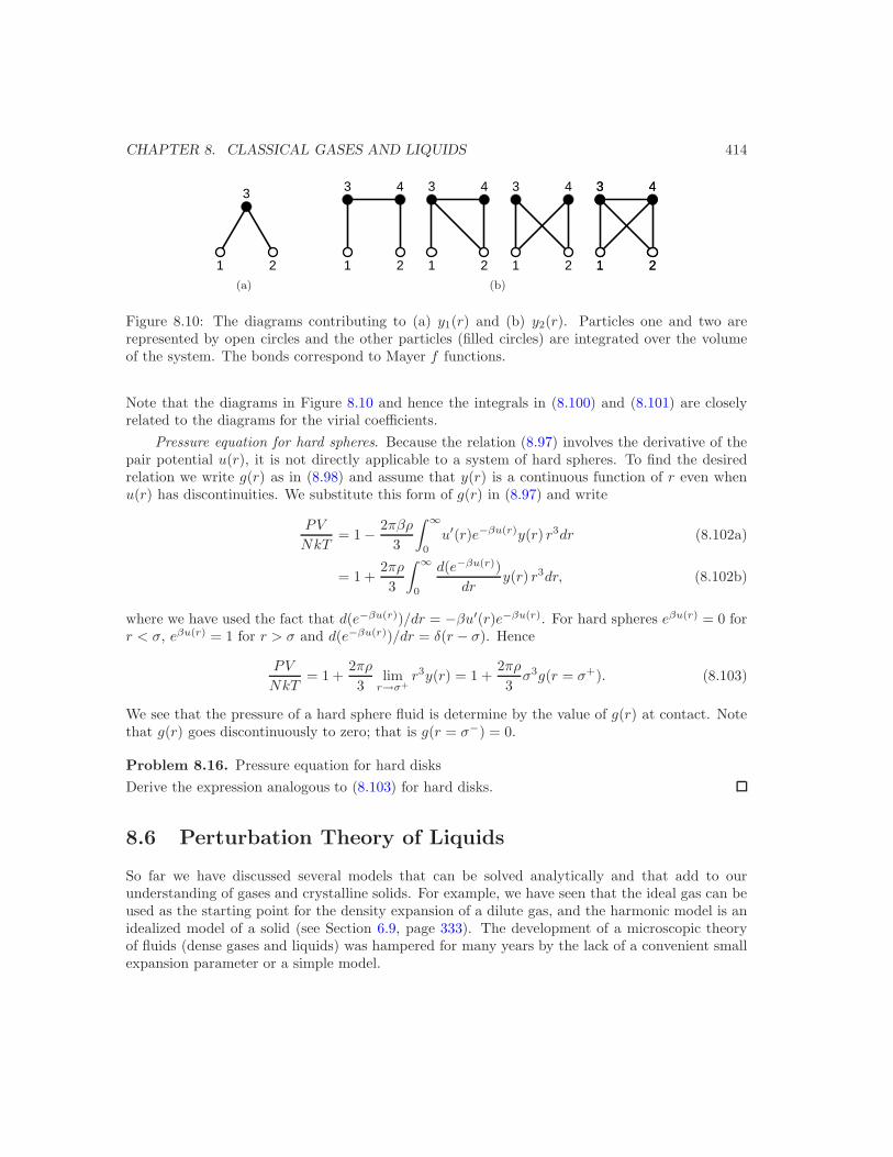
with y0(r) = 1. It is convenient to consider the function y(r) defined by (8.98) instead of thefunction g(r) because y(r) is more slowly varying. The diagrams for y(r) have two fixed pointsrepresented by open circles corresponding to particles 1 and 2. The other particles are integratedover the volume of the system. The diagrams for y1(r) and y2(r) are shown in Figure 8.10. Thecorresponding integrals are
y1(r) =
∫
f(r13)f(r23) dr3, (8.100)
and
y2(r) =1
2
∫
[2f13f34f42 + 4f13f34f42f32 + f13f42f32f14
+ f13f34f42f32f14] dr3dr4. (8.101)
CHAPTER 8. CLASSICAL GASES AND LIQUIDS 414
1 2
3
(a)
1 2
3 4
1 2
3 4
1 2
3 4
1 2
3 4
1 2
3 4
(b)
Figure 8.10: The diagrams contributing to (a) y1(r) and (b) y2(r). Particles one and two arerepresented by open circles and the other particles (filled circles) are integrated over the volumeof the system. The bonds correspond to Mayer f functions.
Note that the diagrams in Figure 8.10 and hence the integrals in (8.100) and (8.101) are closelyrelated to the diagrams for the virial coefficients.
Pressure equation for hard spheres. Because the relation (8.97) involves the derivative of thepair potential u(r), it is not directly applicable to a system of hard spheres. To find the desiredrelation we write g(r) as in (8.98) and assume that y(r) is a continuous function of r even whenu(r) has discontinuities. We substitute this form of g(r) in (8.97) and write
PV
NkT= 1 − 2πβρ
3
∫ ∞
0
u′(r)e−βu(r)y(r) r3dr (8.102a)
= 1 +2πρ
3
∫ ∞
0
d(e−βu(r))
dry(r) r3dr, (8.102b)
where we have used the fact that d(e−βu(r))/dr = −βu′(r)e−βu(r). For hard spheres eβu(r) = 0 forr < σ, eβu(r) = 1 for r > σ and d(e−βu(r))/dr = δ(r − σ). Hence
PV
NkT= 1 +
2πρ
3limr→σ+
r3y(r) = 1 +2πρ
3σ3g(r = σ+). (8.103)
We see that the pressure of a hard sphere fluid is determine by the value of g(r) at contact. Notethat g(r) goes discontinuously to zero; that is g(r = σ−) = 0.
Problem 8.16. Pressure equation for hard disks
Derive the expression analogous to (8.103) for hard disks.
8.6 Perturbation Theory of Liquids
So far we have discussed several models that can be solved analytically and that add to ourunderstanding of gases and crystalline solids. For example, we have seen that the ideal gas can beused as the starting point for the density expansion of a dilute gas, and the harmonic model is anidealized model of a solid (see Section 6.9, page 333). The development of a microscopic theoryof fluids (dense gases and liquids) was hampered for many years by the lack of a convenient smallexpansion parameter or a simple model.
CHAPTER 8. CLASSICAL GASES AND LIQUIDS 415
Simulations of simple liquids have led to the realization that the details of the weak attractivepart of the interparticle interaction and the details of the repulsive part of the interaction alsoare unimportant. As you found in Problem 8.15, the radial distribution function g(r) of a densefluid does not depend strongly on the temperature, and the radial distribution function g(r) for asystem of hard spheres is a good approximation to g(r) for a Lennard-Jones system at the samedensity. Moreover, we can simulate hard sphere systems relatively easily and obtain essentiallyexact solutions for g(r) and the equation of state.
The picture of a dense fluid that is suggested by simulations suggests that the repulsive partof the interaction dominates its structure, and the attractive part of the interaction can be treatedas a perturbation. In the following we will develop a perturbation theory of liquids in which theunperturbed or reference system is taken to be a system of hard spheres (or disks) rather than anideal gas. The idea is that the difference between the hard sphere interaction and a more realisticinteraction can be used as an effective expansion parameter.
We begin by writing the potential energy as
U = U0 + U , (8.104)
where U0 is the potential energy of the reference system, and U will be treated as a perturbation.The configurational integral QN is given by
QN =
∫
· · ·∫
e−β(U0+U) dr1 . . . drN . (8.105)
We multiply and divide the right-hand side of (8.105) by
Q0 =
∫
· · ·∫
e−βU0 dr1 . . . drN , (8.106)
and write
QN =
∫
· · ·∫
e−βU0 dr1 . . . drN
∫
· · ·∫
e−β(U0+U)dr1 . . . drNQ0
(8.107a)
= Q0
∫
· · ·∫
P0 e−βU dr1 . . . drN , (8.107b)
where
P0 =e−βU0
Q0. (8.108)
We see that we can express QN in (8.107b) as the average of exp(−βU) over the referencesystem. We write
QN = Q0
⟨
e−βU⟩
0, (8.109)
and
− βF = ln⟨
e−βU⟩
0=
∞∑
n=1
(−β)nMn
n!. (8.110)
The brackets⟨
. . .⟩
0denote an average over the microstates of the reference system weighted by the
probability P0. We have written M rather than M to distinguish the cumulants for an arbitrary
CHAPTER 8. CLASSICAL GASES AND LIQUIDS 416
reference system from the cumulants defined in Section 8.4.2 for the ideal gas reference system.Note the formal similarity between (8.110) and the expression for Fc in (8.8) and the cumulantexpansion in (8.48).
Problem 8.17. Ideal gas as a reference system
(a) Compare the form of (8.109) and (8.110) for an arbitrary reference system to the form of (8.7)and (8.8), respectively.
(b) Show that if we choose the reference system to be an ideal gas, the expressions (8.109) and(8.110) reduce to (8.7) and (8.8).
We now evaluate the first cumulant M1 in a manner similar to that done to evaluate M1 in(8.49) for a dilute gas. The leading term in (8.110) is
M1 =⟨
U⟩
0=
N∑
i<j=1
⟨
u(rij)⟩
0, (8.111a)
=N(N − 1)
2
1
Q0
∫
· · ·∫
e−βU0 u(r12) dr1 . . . drN . (8.111b)
The radial distribution function of the reference system is given by (see (8.81))
ρ2g0(r12) = N(N − 1)
∫
e−βU0 dr3 . . . drNQ0
. (8.112)
Hence, we can write M1 as
M1 =ρ2
2
∫
u(r12)g0(r12) dr1dr2 (8.113a)
=ρN
2
∫
u(r)g0(r) dr, (8.113b)
and
F = F0 +ρN
2
∫
u(r)g0(r) dr, (8.114)
where F0 in (8.114) is the free energy of the reference system. Note that the form of M1 in (8.113b)is similar to the form of M1 in (8.51b). The difference is that we have included the correlationbetween the particles due to their interaction in (8.113b).
8.6.1 The van der Waals equation
The idea that the structure of a simple liquid is determined primarily by the repulsive part ofthe potential is not new and is the basis of the van der Waals equation of state. We now showhow the van der Waals equation of state can be derived from the perturbation theory we havedeveloped by choosing the reference system to be a system of hard spheres and making somesimple approximations.

CHAPTER 8. CLASSICAL GASES AND LIQUIDS 417
We first assume that g0 has the simple form
g0(r) =
{
0 r < σ
1 r ≥ σ.(8.115)
This approximate form for g0(r) gives
M1 = 2πρN
∫ ∞
σ
u(r) r2dr = −ρaN, (8.116)
where (see (8.35))
a = −2π
∫ ∞
σ
u(r) r2dr. (8.117)
The simplest approximation for F0 is to assume that the effective volume available to a particlein a fluid is smaller than the volume available in an ideal gas. In this spirit we assume that F0 hasthe same form as it does for an ideal gas (see ((6.26), page 299) with V replaced by Veff . We write
F0
NkT= −
[
lnVeff
N+
3
2ln
(2πmkT
h2
)
+ 1]
, (8.118)
whereVeff = V − V0, (8.119)
and
V0 = Nb =1
2N
4πσ3
3. (8.120)
In (8.120) we have accounted for the fact that only half of the volume of a sphere can be assignedto a given particle. The corresponding equation of state with these approximations for M1, F0,and Veff is given by
PV
NkT=
1
1 − bρ− aρ
kT. (8.121)
Equation (8.121) is the familiar van der Waals equation of state. The latter gives results that arein qualitative, but not quantitative agreement with experiment. From the simple approximationswe have made for g0(r) and F0 we can do better.
A much more accurate approximation for the equation of state of liquids is known as theWeeks-Chandler-Andersen theory (see the references). In this approach the interparticle potentialis separated into a reference part and a perturbative part. One way is to separate the potentialinto positive and negative contributions. This choice implies that we should separate the Lennard-Jones potential at r = σ. Another way is to separate the potential at r = 21/6σ so that theforce is separated into positive and negative contributions. This choice is the one adopted by theWeeks-Chandler-Andersen theory. The Lennard-Jones potential is expressed as
uLJ(r) = u0(r) + u(r), (8.122)
CHAPTER 8. CLASSICAL GASES AND LIQUIDS 418
where
u0(r) =
{
uLJ(r) + ǫ r < 21/6σ
0 r ≥ 21/6σ(8.123a)
u(r) =
{
−ǫ r < 21/6σ
uLJ(r) r ≥ 21/6σ(8.123b)
We have added and subtracted ǫ to uLJ(r) for r < 21/6σ so that u0(r) and u(r) are continuous.
Problem 8.18. Qualitative behavior of u(r)
Plot the dependence of u(r) on r and confirm that u(r) is a slowly varying function of r.
Because the reference system in the Weeks-Chandler-Andersen theory is not a system of hardspheres, further approximations are necessary, and the reference system is approximated by hardspheres with a temperature and density-dependent diameter. One way to determine the effectivediameter is to require that the function y(r) defined in (8.98) be the same for hard spheres and forthe repulsive part (8.123a) of the potential. The details will not be given here. What is importantto understand is that a successful perturbation theory of dense gases and liquids now exists basedon the use of a hard sphere reference system.
8.7 *The Ornstein-Zernicke Equation and Integral Equa-tions for g(r)
As mentioned in Section 8.5, we can derive a density expansion for the function y(r), which isrelated to g(r) by (8.98). However, a better approach is to expand a related function that isshorter range. Such a function is the direct correlation function c(r).
To define c(r) it is convenient to first define the pair correlation function h(r) by the relation
h(r) = g(r) − 1. (8.124)
Because g(r) → 1 for r ≫ 1, h(r) → 0 for sufficiently large r. Also h(r) = 0 for an ideal gas.These two properties makes it easier to interpret h(r) rather than g(r) in terms of the correlationsbetween the particles due to their interaction.
We define c(r) by the relation (for a homogeneous and isotropic system):
h(r) = c(r) + ρ
∫
c(|r − r′|)h(r′) dr′. (Ornstein-Zernicke equation) (8.125)
The relation (8.125) is known as the Ornstein-Zernicke equation. Equation (8.125) can be solvedrecursively by first substituting h(r) = c(r) on the right-hand side and then repeatedly substitutingthe resultant solution for h(r) on the right-hand side to obtain
h(r) = c(r) + ρ
∫
c(|r − r′|) c(r′) dr′
+ ρ2
∫∫
c(|r − r′|) c(|r′ − r′′|)c(|r′′ − r′|) dr′dr′′ + · · · (8.126)

CHAPTER 8. CLASSICAL GASES AND LIQUIDS 419
The interpretation is that the correlation h(r) between particles 1 and 2 is due to the directcorrelation between 1 and 2 and the indirect correlation due to increasing numbers of intermediateparticles. This interpretation suggests that the range of c(r) is comparable to the range of thepotential u(r), and that h(r) is longer ranged than u(r) due to the effects of the indirect correlations.That is, c(r) usually has a much shorter range than h(r) and hence g(r).9
Because the right-hand side of the Ornstein-Zernicke equation involves a convolution integral(see (A.11), page 476), we know that we can find c(r) from h(r) by introducing the Fouriertransforms
c(k) =
∫
c(r) eik·r dr, (8.127)
and
h(k) =
∫
h(r) eik·r dr. (8.128)
We take the Fourier transform of both sides of (8.125) and find that
h(k) = c(k) + ρ c(k)h(k), (8.129)
or
c(k) =h(k)
1 + ρh(k), (8.130)
and
h(k) =c(k)
1 − ρc(k). (8.131)
∗Problem 8.19. Properties of c(r)
(a) Write c(r) = c0(r) + ρc1(r) + . . ., and show that c0(r) = f(r) and c1(r) = f(r)y1(r), wherey1(r) is given in (8.100).
(b) We know that g(r) ≈ −βu(r) for βu(r) ≪ 1, as is the case for large r. Show that c(r) = −βu(r)for large r. Hence in this limit the range of c(r) is comparable to the range of the potential.
The Ornstein-Zernicke equation can be used to obtain several approximate integral equationsfor g(r) that are applicable to dense fluids. The most useful of these equations for systems withshort-range interactions is the Percus-Yevick equation. This equation corresponds to ignoring an(infinite) subset of diagrams (and including another subset), but a discussion of these diagramsdoes not add much physical insight.
One way to motivate the Percus-Yevick equation is to note that the lowest order densitycontributions to c(r) are c0(r) = f(r)y0(r) and c1(r) = f(r)y1(r) (see Problem 8.19), wherey0(r) = 1. We assume that this relation between c(r) and y(r) holds for all densities:
c(r) ≈ f(r)y(r) =[
1 − eβu(r)]
g(r). (8.132)
9This assumption does not hold near the critical point.
CHAPTER 8. CLASSICAL GASES AND LIQUIDS 420
Equation (8.132) is correct to first order in the density. If we substitute the approximation (8.132)into the Ornstein-Zernicke equation (8.125), we obtain the Percus-Yevick equation:
y(r) = 1 + ρ
∫
f(r′)y(r′)h(|r − r′|) dr′. (Percus-Yevick equation) (8.133)
We can alternatively express (8.133) as
eβu(r)g(r) = 1 + ρ
∫
[
1 − eβu(r′)]
g(r′)[
g(|r − r′|) − 1]
dr′. (8.134)
Equations (8.133) and (8.134) are examples of nonlinear integral equations.
In general, the Percus-Yevick must be solved numerically. However, it can be solved ana-lytically for hard spheres (but not for hard disks). The analytical solution of the Percus-Yevickequation for hard spheres can be expressed as
c(r) =
− 1
(1 − η)4[
(1 − 2η)2 − 6η(1 + 12η)
2(r/σ) + 12η(1 + 2η)2(r/σ)2
]
(r < σ)
0, (r > σ).(8.135)
Note that the range of c(r) is equal to σ and is much less than the range of g(r).
Given c(r), we can find g(r) by solving the Ornstein-Zernicke equation. The derivation istedious, and we give only the result for g(r) at contact:
g(r = σ+) =1 + 1
2η
(1 − η)2. (8.136)
We can use (8.136) and (8.103) to obtain the corresponding approximate virial equation ofstate for hard spheres. The result is
PV
NkT=
1 + 2η + 3η2
(1 − η)2. (virial equation of state) (8.137)
An alternative way of calculating the pressure is to use the compressibility relation (see (8.200))
1 + ρ
∫
[g(r) − 1] dr = ρkTκ, (8.138)
which can be expressed as (see Section 8.9.3)
(
kT∂ρ
∂P
)−1
= 1 − ρ
∫
c(r) dr. (8.139)
If we substitute the Percus-Yevick result (8.135) into (8.139) and integrate, we find
PV
NkT=
1 + η + η2
(1 − η)3. (compressibility equation of state) (8.140)
If the Percus-Yevick equation were exact, the two ways of obtaining the equation of state wouldyield identical results. That is, the Percus-Yevick equation is not thermodynamically consistent.
CHAPTER 8. CLASSICAL GASES AND LIQUIDS 421
It is interesting that the Carnahan-Starling equation of state for hard spheres (8.71) can be foundby a weighted average of the two approximate equations of state:
PV
NkT=
1
ρkT
[1
3Pv +
2
3Pc
]
, (8.141)
where Pv and Pc are given by (8.137) and (8.140), respectively. The Carnahan-Starling equationof state gives better results than either (8.137) or (8.140).
The Percus-Yevick equation gives reasonable results for g(r) and the equation of state forfluid densities. However, it predicts finite pressures for ηmax ≤ η < 1, even though the maximumpacking fraction ηmax =
√2π/6 ≈ 0.74 (see Problem 8.13).
Problem 8.20. Virial equation of state
Use the form of g(r = σ+) given in (8.136) and the relation (8.103) to derive (8.137) for thepressure equation of state as given by the Percus-Yevick equation.
Another simple closure approximation for the Ornstein-Zernicke equation can be motivatedby the following considerations. Consider a fluid whose particles interact via a pair potential ofthe form
u(r) =
{
∞ (r < σ)
v(r) (r > σ),(8.142)
where v(r) is a continuous function of r. Because u(r) = ∞ for r < σ, g(r) = 0 for r < σ. Forlarge r the Percus-Yevick approximation for c(r) reduces to
c(r) = −βv(r). (8.143)
The mean spherical approximation is based on the assumption that (8.143) holds not just for larger, but for all r. The mean spherical approximation is
c(r) = −βv(r) (r > σ) (8.144a)
and
g(r) = 0, (r < σ) (8.144b)
together with the Ornstein-Zernicke equation.
The hypernetted-netted chain approximation is another useful integral equation for g(r). It isequivalent to setting
c(r) = f(r)y(r) + y(r) − 1 − ln y(r). (hypernetted chain equation) (8.145)
If we analyze the Percus-Yevick and the hypernetted-chain approximations in terms of a di-agrammatic expansion (see Problem 8.34), we that the hypernetted-chain approximation includesmore diagrams than the Percus-Yevick approximation. However, it turns out that the Percus-Yevick approximation is more accurate for hard spheres and other short-range potentials. Incontrast, the hypernetted-chain approximation is more accurate for systems with long-range inter-actions.

CHAPTER 8. CLASSICAL GASES AND LIQUIDS 422
8.8 *One-Component Plasma
We found in Problem 8.7 that the second virial coefficient does not exist if the interparticle potentialu(r) decreases less rapidly than 1/r3 for large r. For this reason we expect that a density expansionof the free energy and other thermodynamic quantities is not applicable to a gas consisting ofcharged particles interacting via the Coulomb potential u(r) ∝ 1/r. We say that the Coulombpotential is long-range because its second moment
∫
r2u(r)r2dr diverges for large r. The divergenceof the second virial coefficient for the Coulomb potential divergence is symptomatic of the fact thata density expansion is not physically meaningful for a system of particles interacting via a long-range potential.
The simplest model of a system of particles interacting via the Coulomb potential is a gasof mobile electrons moving in a fixed, uniform, positive background. The charge density of thepositive background is chosen to make the system overall neutral. Such a system is known as anelectron gas or a one-component plasma (OCP in the literature).
Problem 8.21. Fourier transform of the Coulomb potential
The interaction potential between two particles of charge q is u(r) = q2/r. Show that the Fouriertransform of u(r) is given by
u(k) =4πq2
k2. (8.146)
First find the Fourier transform of1
rer/λ and then take the limit λ→ 0.
Debye-Huckel theory. Debye and Huckel developed a mean-field theory that includes theinteractions between charged particles in very clever, but approximate way. Consider an electronat r = 0 of charge −q. The average electric potential φ(r) in the neighborhood of r = 0 is givenby Poisson’s equation:
∇2φ(r) = −4π[
(negative point charge at origin) + (density of positive uniform background)
+ (density of other electrons)]
. (8.147a)
That is,
∇2φ(r) = −4π[
− qδ(r) + qρ− qρg(r)]
, (8.147b)
where ρ is the mean number density of the electrons and the uniform positive background, andρg(r) is the density of the electrons in the vicinity of r = 0. Equation (8.147b) is exact, but wehave not specified g(r). The key idea is that g(r) is approximately given by the Boltzmann factor(see (8.73))
g(r) ≈ eβqφ(r). (8.148)
If we combine (8.147b) and (8.148), we obtain the Poisson-Boltzmann equation for φ(r):
∇2φ(r) = −4πq[
− δ(r) + ρ− ρ eqβφ(r)]
. (8.149)
For βqφ≪ 1, we may write e−βqφ(r) ≈ 1−βqφ(r) and obtain the linearized Poisson-Boltzmannequation
(∇2 − κ2D)φ(r) = 4πq δ(r), (8.150)
CHAPTER 8. CLASSICAL GASES AND LIQUIDS 423
where κ2D is given by
κ2D = 4πβρq2. (8.151)
The solution to (8.150) that is spherically symmetric can be shown to be (see (9.22), page 440)
φ(r) = −q e−r/λD
r, (8.152)
where λD = 1/κD. The energy of the other elections in the potential φ(r) is ueff(r) = −qφ(r) sothat the effective energy of interaction between two electrons is given by
ueff(r) = q2e−r/λD
r. (8.153)
The result (8.153) shows that the electrons collaborate in such a way as to screen the potentialof a given electron over a distance λD. The quantity λD is called the Debye screening length andis the radius of the cloud of the electrons about any one electron that act to screen the Coulombpotential. The screening of the charge of the electrons is another example of a cooperative effect.
Note that to use statistical arguments, it is necessary that many particles have approximatelythe same potential energy, that is, many particles need to be within the range λD of φ. Thisrequirement can be written as ρλ3
D ≫ 1. This condition holds in the limit of low density and hightemperature.
Problem 8.22. Range of validity of the Debye-Huckel theory
Show that the condition ρλ3D ≫ 1 is equivalent to the condition that the mean interaction energy
between two electrons e2/(r = λD) be much smaller than the mean kinetic energy.
We now determine the radial distribution function g(r) and the thermodynamic properties ofthe one-component plasma. From (8.148) we have
g(r) = eβqφ(r) ≈ 1 − βqφ(r) = 1 − βq2
re−r/λD . (8.154)
Problem 8.23. Thermodynamic properties of the Debye-Huckel theory
(a) The total energy per particle of the one-component plasma is given by
E
N=
3
2NkT +
ρ
2
∫
[g(r) − 1]u(r) dr. (8.155)
The factor of g − 1 rather than g in the integrand is due to the uniform positive background.Use the approximation (8.154) to show that the mean energy per particle can be expressed as
E
N=
3
2kT − 1
2
e2
λD= kT
[3
2− 1
2
e2
λDkT
]
= kT[3
2− ǫ
2
]
, (8.156)
where the dimensionless parameter ǫ is defined as
ǫ ≡ e2
λDkT. (8.157)
CHAPTER 8. CLASSICAL GASES AND LIQUIDS 424
(b) Find a expression similar to (8.156) for the mean pressure.
The form of the right-hand side of (8.156) suggests that the Debye-Huckel theory is equivalentto keeping the first term in an expansion in powers of ǫ, in analogy to the expansion in powers ofthe density for systems with short-range interactions. However, the expansion is more complicatedand involves logarithmic terms in ǫ. For example, the next order terms are proportional to ǫ2 andǫ2 ln ǫ.
Problem 8.24. The Debye-Huckel approximation of the direct correlation function
Use the form (8.154) to find the corresponding Fourier transform h(k). Then use (8.130) to showthat the direct correlation function c(k) in the Debye-Huckel approximation is given by
c(k) = −βu(k). (8.158)
Hence the Debye-Huckel approximation is equivalent to approximating the direct correlation func-tion c(r) by −βu(r), the result for c(r) to lowest order in the potential (see Problem 8.19b).
∗Diagrammatic expansion. We derived the density expansion of the free energy by first doinga high temperature expansion (see Section 8.4.2). Although individual terms in this expansiondiverge at short separations for systems with a strongly repulsive interaction, we found that thedivergence was removed by rearranging the expansion so that all terms of a given density aregrouped together and summed.
As we have discussed, an expansion in terms of the density and the interaction of smallnumbers of particles makes no sense if the interaction is long range. We now discuss how to groupindividual terms in the high temperature expansion so that the divergence at large separations dueto the long-range nature of the Coulomb potential is removed.10
Instead of considering the diagrammatic expansion for the free energy, we consider the hightemperature expansion for g(r), because the latter is easier to interpret physically. It is convenientto write g(r) in the form
g(r) = e−βψ(r), (8.159)
where ψ(r) is the potential of mean force. Note that ψ(r) reduces to u(r) in the limit of lowdensities. Recall that we obtained the low density expansion by first summing all possible potential(u) bonds between two particles. That is, we summed the infinite class of diagrams with themaximum number of bonds for a given number of particles. Because the Coulomb interaction islong-range, it is plausible that we should first sum the infinite class of diagrams corresponding tothe maximum number of particles for a given number of bonds. These diagrams are called ring
diagrams. The first several ring diagrams are shown in Figure 8.11. Because we know that theCoulomb interaction is screened, we expect that we should add up the contributions of all the ringdiagrams before we include the contributions of other diagrams.
The contribution of the ring diagrams to ψ(r) is given by
− βψ(r) = −βu(r) + ρ
∫
[−βu(r13)][−βu(r32)] dr3
+ ρ2
∫
[−βu(r13)][−βu(r34)][−βu(r42)] dr3 dr4 + . . . , (8.160)
10Important early work was done by J. E. Mayer, “The theory of ionic solutions,” J. Chem. Phys. 18, 1426–1436(1950).

CHAPTER 8. CLASSICAL GASES AND LIQUIDS 425
Figure 8.11: The first several ring diagrams for ψ(r). The bonds represent the Coulomb interactionu(r) = e2/r.
where r = |r1−r2|. The structure of the integrals in (8.160) is the same as the convolution integraldiscussed in Section 8.9.1. We follow the same procedure and take the spatial Fourier transformof both sides of (8.160). The result can be written as
− βψ(k) = −βu(k) + ρ[−βu(k)]2 + ρ2[−βu(k)]3 + . . . , (8.161)
where u(k) is the Fourier transform of u(r) = e2/r (see Problem 8.146). Because the terms in(8.161) form a geometric series, we obtain
−βψ(k) =−βu(k)
1 + ρβu(k)=
−β4πe2
k2 + βρ4πe2(8.162a)
= −β 4πe2
k2 + κ2D
, (8.162b)
where κD is given by (8.151). Hence
ψ(k) =4πe2
k2 + κ2D
(8.163)
and
ψ(r) =βe2
rǫ−κDr. (8.164)
From (8.164) we see that the effective interaction is the Debye-Huckel screened potential as ex-pected.
8.9 Supplementary Notes
8.9.1 The third virial coefficient for hard spheres
The third virial coefficient B3 is given by (see (8.10b))
B3 = − 1
3V
∫
f(|r1 − r2|)f(|r1 − r3|)f(|r2 − r3|) dr1dr2dr3. (8.165)
B3 can be calculated for hard spheres by geometrical considerations, but these considerations testone’s geometrical intuition. An easier way is to take advantage of the fact that (8.165) is an

CHAPTER 8. CLASSICAL GASES AND LIQUIDS 426
example of a convolution integral (see Section A.11) and can be expressed in terms of the Fouriertransform of f(r).
Problem 8.25. Evaluation of B3 for hard spheres
(a) Read Appendix A.11 on convolution integrals and show that B3 in (8.165) can be expressedas
B3 = −1
3
∫
d3k
(2π)3f(k)3, (8.166)
where f(k) is the Fourier transform of f(r).
(b) Use (A.46) and the form of f(r) for hard spheres,
f(r) =
{
−1 (0 < r < σ)
= 0 (r > σ),(8.167)
to show that
f(k) = 4πσ3
[
cos kσ
(kσ)2− sin kσ
(kσ)3
]
. (8.168)
(c) *The integral in (8.166) with (8.168)for f(k) can be evaluated numerically or calculated ana-lytically. The result is
B3 =5π2
18σ6. (hard spheres) (8.169)
B4 can also be evaluated analytically for hard spheres, but higher order virial coefficients haveto be evaluated by Monte Carlo methods.
8.9.2 Definition of g(r) in terms of the local particle density
Another way of defining g(r) is in terms of the local particle density. Given the properties of thedelta function δ(x− x0) (see Section A.10), we have that
x0+ǫ∫
x0−ǫ
δ(x − x0) dx = 1, (8.170)
and the integral over any other values of x gives zero. Hence, the integral of the sum∑N
i=1 δ(r−ri)about r over the volume element dr gives the number of particles in the volume element. We definethe local particle density
ρ(r) =N
∑
i=1
δ(r − ri), (8.171)
and the single particle density function

CHAPTER 8. CLASSICAL GASES AND LIQUIDS 427
ρ1(r) =⟨
N∑
i=1
δ(r − ri)⟩
, (8.172)
where⟨
δ(r − r1)⟩
is given by
⟨
δ(r − r1)⟩
=1
QN
∫
δ(r − r1) e−βU(r1,...,rN ) dr1 . . . drN (8.173a)
=1
QN
∫
e−βU(r,r2,...,rN ) dr2 . . . drN . (8.173b)
Similarly, the two-particle distribution function ρ2(r1, r2) is defined as
ρ2(r1, r2) =
N∑
i6=j=1
⟨
δ(r1 − ri)δ(r2 − rj)⟩
. (8.174)
We can use the same reasoning as in (8.173) to show that ρ2 as defined in (8.174) can be writtenas
ρ2(r1, r2) = N(N − 1)
∫
e−βU(r1,r2,r3...rN ) dr3 dr4 . . . drN∫
e−βU(r1,r2,r3...rN ) dr1 dr2 dr3 dr4 . . . drN. (8.175)
If we compare (8.175) and (8.81), we see that we can also express g(r1, r2) as
ρ2g(r1, r2) = ρ2(r1, r2) =∑
i6=j
⟨
δ(r1 − ri)δ(r2 − rj)⟩
. (8.176)
Hence, we see that g(r) is related to the spatial correlations of the density fluctuations in thesystem.
Problem 8.26. One particle distribution function
Use the definition (8.172) and the result (8.173b) to show that ρ1(r1) = ρ for a homogeneoussystem. Hint: let rj = r1 + xj for j 6= 1. Note that the denominator becomes independent ofr1.
8.9.3 X-ray scattering and the static structure function
The mean distance between particles in a typical fluid or solid is the order of 10−10 m. Thesewavelengths are available using neutrons or X-rays. To understand how an elastic scatteringexperiment can probe the static correlations between particles we consider X-ray scattering. Aphoton of wavelength of 10−10 m has an energy of ~ω = hc/λ ≈ 104 eV. This energy is verylarge in comparison to the typical energy of the particles in a liquid which is the order of kT orapproximately 0.1 eV at room temperatures. Hence, the collisions of photons with the particles ina liquid and a solid will leave the photon energies almost unchanged and to a good approximation,the scattering can be treated as elastic.
In the following we will show that the scattered intensity I(θ) of the X-rays is given by
I(θ) ∝ NI0S(k), (8.177)

CHAPTER 8. CLASSICAL GASES AND LIQUIDS 428
where the wave vector k is related to the scattering angle θ and I0 is the intensity of the incomingbeam. The static structure function S(k) is defined as
S(k) =1
N
⟨
N∑
i,j=1
eik·(ri−rj)⟩
. (8.178)
In the following we will derive (8.177) and show that the radial distribution function g(r) is relatedto the Fourier transform of S(k).
To obtain (8.177) we assume that the incoming beam is a plane wave of wave vector q.For simplicity we assume that the incident beam is scattered from an atom at the origin. Thescattered signal is measured as a function of θ, the angle between the incident and scattered beams(see Figure 8.12). The detector receives a (spherical) wave of amplitude f(θ)/R, where R is thedistance of the detector from the origin. The form factor f(θ) depends on the detailed physics ofthe scattering process. Because the scattering is elastic, we have |q′| = |q|.
The amplitude of the wave scattered by an atom at ri has a phase difference of (q′ − q) · rirelative to the wave scattered by the atom at the origin. Hence the scattering amplitude fromatom i at ri is proportional to
f(θ)
Reik·ri , (8.179)
wherek = q′ − q. (8.180)
Because the form factor f(θ) is the same for all atoms, the total scattering amplitude is the sum
A(θ) =f(θ)
R
∑
i
eik·ri . (8.181)
The detector measures the thermal average of the scattering intensity:
I(θ) =⟨
|A(θ)|2⟩
=|f(θ)|2R2
⟨
∑
i,j
eik·(ri−rj)⟩
=|f(θ)|2R2
NS(k), (8.182)
where the static structure function S(k) is defined in (8.178).
The static structure function S(k) is a measure of the correlations between the positions ofthe atoms in the liquid. We now show that S(k) is related to the Fourier transform of g(r). Wefirst divide the sum over i and j in (8.178) into self, i = j, and distinct, i 6= j, contributions. Thereare N of the former and N(N − 1) of the latter. We have
S(k) = 1 +1
NN(N − 1)
⟨
eik·(r1−r2)⟩
(8.183a)
= 1 +N(N − 1)
N
∫
eik·(r1−r2) e−βUdr1 . . . drN∫
e−βU dr1 . . . drN. (8.183b)
If we use the definition (8.81) of g(r1, r2), we can write (8.183b) as
S(k) = 1 +1
N
∫
ρ2g(r1, r2) eik·(r1−r2)dr1dr2. (8.184)
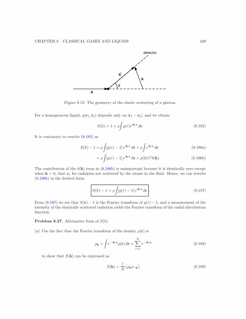
CHAPTER 8. CLASSICAL GASES AND LIQUIDS 429
q
kq′
θ
detector
Figure 8.12: The geometry of the elastic scattering of a photon.
For a homogeneous liquid, g(r1, r2) depends only on |r1 − r2|, and we obtain
S(k) = 1 + ρ
∫
g(r)eik·r dr. (8.185)
It is customary to rewrite (8.185) as
S(k) − 1 = ρ
∫
[g(r) − 1] eik·r dr + ρ
∫
eik·r dr (8.186a)
= ρ
∫
[g(r) − 1] eik·r dr + ρ(2π)3δ(k). (8.186b)
The contribution of the δ(k) term in (8.186b) is unimportant because it is identically zero exceptwhen k = 0, that is, for radiation not scattered by the atoms in the fluid. Hence, we can rewrite(8.186b) in the desired form:
S(k) − 1 = ρ
∫
[g(r) − 1] eik·r dr . (8.187)
From (8.187) we see that S(k) − 1 is the Fourier transform of g(r) − 1, and a measurement of theintensity of the elastically scattered radiation yields the Fourier transform of the radial distributionfunction.
Problem 8.27. Alternative form of S(k)
(a) Use the fact that the Fourier transform of the density ρ(r) is
ρk =
∫
e−ik·rρ(r) dr =
N∑
i=1
e−ik·ri (8.188)
to show that S(k) can be expressed as
S(k) =1
N
⟨
ρkρ−k
⟩
. (8.189)

CHAPTER 8. CLASSICAL GASES AND LIQUIDS 430
(b) Use (8.189) to show that S(k) can be written as
S(k) =1
N
⟨
N∑
i=1
N∑
j=1
e−ik·rieik·rj⟩
(8.190)
=1
N
⟨∣
∣
N∑
i=1
e−ik·ri∣
∣
2⟩. (8.191)
Compressibility equation. In a scattering experiment the beam samples a subset of the totalvolume. Because the number of particles in the subset fluctuates, we need to use the grandcanonical ensemble to describe the measured value of S(k). The energy and pressure equations(8.74) and (8.97) are identical in both ensembles, but the compressibility equation holds only inthe grand canonical ensemble because it relates the integral of g(r) − 1 and hence S(k = 0) tofluctuations in the density.
In Section 6.11 we derived the relation between the isothermal compressibility and the density(number) fluctuations (see (6.238), page 343):
ρκ =1
kT
⟨
N2⟩
−⟨
N⟩2
⟨
N⟩ . (8.192)
We now relate the integral over g(r) to the density fluctuations. In the grand canonical ensemblethe probability density of finding n particular particles with positions r1, . . . , rn in the rangedr1, . . . , drn is given by
Pn(r1, . . . , rn) =
∞∑
N=0
zN
N !ZG
∫
e−βUN drn+1 . . . drN , (8.193)
where z = eβµ. There are N(N − 1) . . . (N −n+ 1) = N !/(N −n)! different sets of particles whichcan correspond to the n particles. Hence, the total probability that any n particles occupy thesevolume elements is given by
Pn(r1, . . . , rn) ≡ ρng(r1, . . . , rn), (8.194a)
=
∞∑
N=0
zN
N − n)!ZG
∫
· · ·∫
e−βUN drN+1, . . . drN . (8.194b)
From the definition of P1 and P2, it follows that
∫
P1(r1) dr1 =⟨
N⟩
, (8.195)
and∫∫
P2(r1, r2) dr1dr2 =⟨
N(N − 1)⟩
. (8.196)
CHAPTER 8. CLASSICAL GASES AND LIQUIDS 431
We can use (8.196) and (8.195) to obtain
∫∫
[
P2(r1, r2) − P1(r1)P1(r2)]
dr1dr2 =⟨
N2⟩
−⟨
N⟩2 −
⟨
N⟩
. (8.197)
The left-hand side of (8.197) is equal to V ρ2∫
[g(r) − 1] dr for a homogeneous system. Hence weobtain
Nρ
∫
[g(r) − 1] dr =⟨
N2⟩
−⟨
N⟩2 −
⟨
N⟩
, (8.198)
or
1 + ρ
∫
[g(r) − 1] dr =
⟨
N2⟩
−⟨
N⟩2
⟨
N⟩ . (8.199)
If we use the relation (8.192), we find the desired relation
1 + ρ
∫
[g(r) − 1] dr = ρkTκ. (compressibility equation) (8.200)
The relation (8.200), known as the compressibility equation, expresses the isothermal compressibil-ity κ as an integral over g(r) and holds only in the grand canonical ensemble. From the relation(8.187) we have
S(k = 0) − 1 = ρ
∫
[g(r) − 1] dr, (8.201)
and hence
S(k = 0) = ρkTκ. (8.202)
Problem 8.28. Value of S(k = 0) in different ensembles
As mentioned, the condition (8.202) on S(k = 0) only applies in the grand canonical ensemble.What is S(k = 0) in the canonical ensemble? Why is the value of S(k = 0) different in these twoensembles?
Alternative form of the compressibility relation. Finally, we express the compressibility relation(8.138) in terms of c(r) rather than h(r) = g(r)−1 by using the Ornstein-Zernicke equation (8.125).We write the latter as
g(r) − 1 = c(r) + ρ
∫
c(|r − r′|)[g(r′) − 1]dr′. (8.203)
and multiply both sides by dr and integrate noting that∫
c(|r − r′|) dr =∫
c(r) dr. We thenrearrange the results to find
∫
[g(r) − 1] dr =
∫
c(r) dr
1 − ρ∫
c(r) dr. (8.204)
Finally we combine (8.204) with (8.138) to find (8.139).

CHAPTER 8. CLASSICAL GASES AND LIQUIDS 432
8.10 Vocabulary
density expansion, virial coefficients, cluster integrals
Mayer f function
cumulant, high temperature expansion
disconnected, reducible, and irreducible diagrams
ladder diagrams, ring diagrams
radial distribution function g(r)
static structure function S(k)
reference theory of liquids
Debye-Huckel theory
Additional Problems
Problem 8.29. Why is the method that we have used to obtain the virial expansion for a classicalfluid not applicable to a quantum system?
Problem 8.30. Temperature dependence of B2
(a) A simpler potential that captures some of the properties of the Lennard-Jones potential is thesquare well potential which is defined as
u(r) =
∞ (r < σ)
−ǫ 0 < r < λσ)
0 (r > λσ),
(8.205)
where σ is the diameter of the hard core part, λσ is the range of the attractive well, and ǫ isthe well depth. Show that for this potential the Mayer function f(r) is given by
f(r) =
−1 (r < σ
g = eβǫ − 1 (r < λσ)
0 (r > λσ),
(8.206)
andB2(T ) =
π
2
[
1 − (λ2 − 1)g]
. (8.207)
(b) Make a plot of the temperature dependence of B2(T ) as given by (8.207) and compare it tothe approximate temperature dependence given by (8.36).
(c) Program SecondVirialCoefficient evaluates the integral over r in (8.32) numerically us-ing a simple numerical method (Simpson’s rule) to determine the T -dependence of B2 forthe Lennard-Jones potential. Compare the numerical results for the Lennard-Jones potentialwith the approximate result in (8.36). At what temperature does B2 vanish? How does thistemperature compare with that predicted by (8.36)?

CHAPTER 8. CLASSICAL GASES AND LIQUIDS 433
Problem 8.31. Inversion temperature of argon
In Section 2.23.2, page 86, we discussed the porous plug or Joule-Thomson process in which agas is forced from a high pressure chamber through a porous plug into a lower pressure chamber.The process occurs at constant enthalpy and the change in temperature of the gas is given bydT = (∂T/∂P )H dP for small changes in pressure. We know that (see (2.218), page 87)
(∂T
∂P
)
H=
1
CP
[
T(∂V
∂T
)
P,N− V
]
. (8.208)
The locus of points (∂T/∂P )H = 0 is called the Joule-Thomson inversion curve. Assume theapproximate equation of state V = NkT/P + NB2 and use your numerical results for B2 fromProblem 8.30 for the Lennard-Jones potential to compute the inversion temperature at which theinversion curve is a maximum. Use σ = 3.4 A and ǫ/k = 120K and compare your result with theexperimental value of 780K.
Problem 8.32. Alternative form of B2
(a) Show that the virial coefficient B2 given in (8.32) can be written in the form
B2 = − 1
6kT
∫ ∞
0
rdu(r)
dre−βu(r)4πr2dr. (8.209)
(b) Assume that g(r) can be written in the form
g(r) = g0 + ρg1(r) + ρ2g2(r) + · · · (8.210)
Use the virial equation of state (8.97) to obtain
PV
NkT= 1 − ρ
6kT
∞∑
n=0
ρn∫ ∞
0
rdu
drgn(r) 4πr2dr. (8.211)
Compare the density expansion (8.9) of PV/NkT with (8.210) and show that
Bn+2 = − 1
6kT
∫ ∞
0
rdu
drgn(r)4πr
2dr. (8.212)
(c) From the result of part (a) show that
g0(r) = e−βu(r). (8.213)
(d) Use the relation (8.97) to find the form of B2 implied by (8.213).
Problem 8.33. Exact equation of state for hard rods
Consider a one-dimensional system of particles confined to a box of length L. The interparticleinteraction is given by
u(x) =
{
∞ (x < σ)
0 (x ≥ σ)(8.214)
This system of hard rods is also known as a Tonks gas.

CHAPTER 8. CLASSICAL GASES AND LIQUIDS 434
(a) Evaluate the virial coefficients B2 and B3. It is possible to do the integrals analytically.
(b) Note that the form of the interaction (8.214) prevents particles from exchanging places, thatis, from changing their order. What is the available “volume” in which the particles can move?Use this consideration to guess the form of the equation of state.
(c) *Calculate the partition function and show that the exact equation of state of a system of hardrods is given by
P
ρkT=
1
1 − η, (8.215)
where η = ρσ and ρ = N/L.
(d) What is the value of the nth virial coefficient that is implied by the form (8.215) of the hardrod equation of state?
∗Problem 8.34. Virial coefficients implied by the Percus-Yevick approximation
Use the approximate results (8.137) and (8.140) for the Percus-Yevick equation of state for hardspheres to determine the virial coefficients implied by the Percus-Yevick equation. How do thesevirial coefficients compare with the exact coefficients given in Table 8.2?
Suggestions for Further Reading
Early work on hard disks was done by B. J. Alder and T. E. Wainwright, “Phase transition inelastic disks,” Phys. Rev. 127, 349–361 (1962). See also A. C. Mitus, H. Weber, and D. Marx,“Local structure analysis of the hard-disk fluid near melting,” Phys. Rev. E 55, 6855–6859(1997).
John A. Barker and Douglas Henderson, “What is “liquid”? Understanding the states of matter,”Rev. Mod. Phys. 48, 587–671 (1976).
R. Brout and P. Carruthers, Lectures on the Many-Electron Problem, Interscience Publishers(1963). Our discussion of cumulants and the virial expansion is based on Chapter 1 of thistext.
D. Chandler, J. D. Weeks, and H. C. Andersen, “The van der Waals picture of liquids, solids andphase transformations,” Science 220, 787–794 (1983).
David Chandler, Introduction to Modern Statistical Mechanics, Oxford University Press (1987).
N. Clisby and B. M. McCoy, “Ninth and tenth order virial coefficients for hard spheres in Ddimensions,” J. Stat. Phys. 122, 15–57 (2006). N. Clisby and B. N. McCoy, “New results forvirial coefficients of hard spheres in D dimensions,” Pramana 64, 775–783 (2005).
Herbert Goldstein, Charles P. Poole, and John L. Safko, Classical Mechanics, third edition,Addison-Wesley (2001).
Jean-Pierre Hansen and Ian R. McDonald, Theory of Simple Liquids, third edition, AcademicPress (2006).

CHAPTER 8. CLASSICAL GASES AND LIQUIDS 435
Mariano Lopez de Haro, Andres Santos, and Santos Bravo Yuste, “A student-oriented derivationof a reliable equation of state for a hard-disc fluid,” Eur. J. Phys. 19, 281–286 (1998).
Joseph Kestin and J. R. Dorfman, A Course in Statistical Thermodynamics, Academic Press(1971). Chapter 7 in this senior/graduate text has a good discussion of the properties of realgases.
Stanislav Labık, Jirı Kolafa, and Anatol Malijevsky, “Virial coefficients of hard spheres and harddisks up to the ninth,” Phys. Rev. E 71, 021105-1–8 (2005).
K. Younge, C. Christenson, A. Bohara, J. Crnkovic, and P. Saulniera, “A model system for exam-ining the radial distribution function,” Am. J. Phys. 72, 1247–1250 (2004). An experimentsuitable for undergraduates that illustrates the meaning of the radial distribution functionfor a system of hard disks is discussed.