Report R82-920009-F

COMPUTATION OF LAMINAR AND TURBULENT FLOW IN 90-DEGREE SQUARE-DUCTAND PIPE BENDS USING THE NAVIER-STOKES EQUATIONS

W. R. Briley, R. C. Buggeln and H. McDonald \Scientific Research Associates, Inc.P.O. Box 498Glastonbury, CT 06033

April 1982

Final Report for Period 1 March 1981 - 28 February 19S2

Approved for Public Release; Distribution UiIfmited

CL ,DTICPrepared for: MAY 10 ?M

OFFICE OF NAVAL RE.SEFARCHLL.t 800 N. Quincy Street

C-40) Arlington, VA 22217 D

82 05-.10 I0,

S4CURITY CLASSIFICATION OF THIS 'E(Wha, Doae Entotwed)

Slength scale. Six different flow cases are considered, c .. ingflow structure and its dependence on geometric and flow paramfT v. -_.LeThe computed results are compared with available experimenta] tts,and the sequence of comparisons helps to establish the accw.,to ay , .n Lchthese flows c.an be predicted by the present method using m., .. att, 'segrids (7 1C,O000 points).

A0cessijn ForNTYS GRA&IDTIC TAB3Unaiaunced r]Justif ~aion .cL_

By-_

Distribi•tion/Availability Codos

Avail and/orDifit Special

SECURITY CLASSIFICATION OF ru,, AGE(Whan Dlata Eri

IPage

7 N1. RODUCTICIN . . . . . . .. . . . . .. . ... . . . . . . . . . . . . . . . 1.

Previous Work ..-. . . . . . . . . . . . . . . .. . 2

THE PRESENT APPROACH . . . . .. . . . ... . . . . . . . . . . . . . . . . . 4

Governing EquaLicns and Coordinate System ............... 4Tur'bu] ence Model. . . .

Phy•iLca-. Boundar, and Initial Conditions ............ ............... 7

SOLUTION PROCEDURE ......................... ............................. 10

Backgr, und ...................... ... ............................. 10Spatial Diffe'encing and Artificial Dissipation ..... ............ .. 11Split LBI Algorithm .......... ........................... 12

Linearization and Time Differencing. ....... ............... ... 12Special Treatment of Diffusive Terms ....... ............... ... 13Consistent Splitting of the LBI Scheme ......... ........... ... 14

COMPUTED RESULTS ..................... .............................. 15

TABLE I ................................................................. 16

Convergence Rate .................... ........................... .. 17

Comparison With Experiment ................ .................... ... 18Flow Structure for Pipe Bend Cases .................. ................ 19Influence of Bouaoary Layer Thickness on Duct Flow .... .......... .. 20

CONCLUDING REMARKS ....................... ........................... .. 21

REFERENCES ........................... ............................... .. 22

FIGURES ............................ .................................. 24

INTRODUCTION

The I low around bends of various cross section and through other curved flow pi.:

!;dges is of conslderable importance in internal flow applications. A very common

UXample Is that of flow through all elbow or other section of curved pipe connecting tw

S.(cLions of straight pipe. Other examples include that of flow in curved ducts of re(

t;angular or other cross section and flow in more general smoothly-curved passages.

Althbough such geometries are unavoidable in many instances to achieve compact and/or

I iglitweight designs, they are sources of complex secondary flows, losses, and variablh.

licit tLransfer rates which may affect overall performance or present other design con-

striaights. In other instances, the presence of geometries which produce high total.

presý;iiru losses or heat tLransfer may be quite intentional, but accompanied by a need

Ior dLtailcd understanding and/or predictive techniques.

The underlying physical mechanisms present in flows of this type are clearly

lctic nodatd by secondary flow theory (reviewed for example by Hawthorne [1,2] and lorlo..1

& lakshmiinarayana [3]). In its simplest form, the secondary flow is generated by tivin i-

hlg a primary flow in which viscous or other forces upstream have produced a non-zero

velocity gradient normal to the plane of curvature. Fluid with above (/below) average

nioiiiei.tuili migrates to the outside (/inside) of the bend as a result of the radial pre;.-

-u're gradients produced by turning the flow. This phenomenon is quantified by second~l'%

I low theory as the generation of streamwise krorticity from transverse vorticity which

has been produced upstream. The secondary velocities are usually quite large (a sub-

t-iait ial fraction of the primary velocity) and are influenced by several factors sucth

.is I low deflection, strength of inlet vorticity, and thickness of shear regions.

Although the secondary flow is generated by an inviscid mechanism, its strength

and subsequent development are influenced in varying degrees by viscous effects.

E'irLhi-rmore, since strong deflections may occur over a short distance, such flows irt,

usually of a transition type and never become fully developed or assume any convenielt

similarLty form. By analogy with external flows, the flow often behaves an an inviscid!

flow In a central core region, with viscous effects limited to regions near solid

boundaries. Unlike most external flow problems, however, the inviscid core region is

often not an irrotational potential flow but is rotational with a complex interaction

occurring between the two flow regions. Furthermore, as the flow passes through suc-

ce0,ssive flow passages, new viscous and thermal boundary layers develop beneath pre-

vious boundary layers, and the distinction between rotational inviscid and viscous

boundary layer regions becomes tenuous.

Previous Work

A number of previous investigations have computed flow through stronngly curved

ducts using approximate forms of the governing equations.

Pratap atLd Spalding [4] have considered turbulent flow in a stron;iv ,_-uvd duc:t

using their "partially parabolic" calculation procedure and a two-equa: ion/walt-fu~ic:LI,.,

Lurbulenlce model. Ghia and Sokhey [5] have computed laminar flow In ducts of strong

curvature using a parabolized form of the Navier-Stokes equations. Kreskovsky, Briley

and McDonald [6] have recently employed an approximate initial-value analysis for

visicous primary and secondary flows to compute laminar and turbulent flow iil strongly

curved ducts, using a one-equation turbulence model with viscous sublayer resolution.

Humphrey, Taylor and Whitelaw [7,8] have obtained laser-Doppler anemometry measurements

of laminar and turbulent flow in a square duct of strong curvature, and also performed

numerical calculations using a version of the fully-elliptic calculation procedure

developed at Imperial College by Gosman, Pun, Patankar and Spalding. Further extensive

'Adculations including heat transfer effects have been made recently by Yee and

1Humphrey [9].

In view of the general complexity of flow in curved ducts and pipes, including

the likely occurrence of flow separation, analysis by numerical solution of the

Navier-Stokes equations is both attractive and viable provided efficient numerical

methods are used. This approach was recently employed by the authors [10,11] co study

laminar and turbulent flow in curved ducts, pipes, and two-dimensional channels. This

study concentrated on the square-duct geometry and flow conditions for which detailed

measurements have been obtained by Taylor, Whitelaw and Yianneskis [12]. In this study,

mesh resolution tests and validation of inflow/outflow boundary conditions were per-

o'rned on tie two-dimensional channel problem. Solutions for laminar and turbulent

flow on corresponding square ducts having the same curvature as the channels were

computed and corpared with measurements from [12]. Good qualitative and reasonable

quantitative agreement between solution and experiment was obtained.

In the present investigation, further extensive calculations were performed

,ising the same computational method as in [10,11]. Six flow cases including both

laminar and turbulent flow in curved pipes and square ducts are evaluated and compared

with available experimental measurements. The laminar square duct of curvature ratio

2.3 (radius of curvature R to hydraulic diameter d) considered in [10,11] was recomputed

to test its sensitivity to the grid distribution and other solution parameters. Two

turbulent calculations for this s.-ur_ geometry, but having different inlet boundary layer

thicknesses are evaluated. One of these cases has a fu ly-developed inflow and was

2

chosen because it is one of the evaluation cases for the 1980-81 Stanford Conference

on Complex Turbulent Flows for ccmparison of computation and experiment. Two pipe

bends are considered;, one laminar and one turbulent, each having a curvature ratio of

2.8. These are compared with the recent measurements of Taylor, Whitelaw and Yianneskis

[131, Finltly, turbulent flow in a sharp elbow of curvature ratio 1.0 is considered.

V

3'

THE PRESENT APPROACH

The present approach is the numerical solution of the compressible Reynolds-

averaged Navier-Stokes equations in the low Mach number regime (M = 0.05) for which

they approximate the flow of a liquid. The governing equations are solved using an

efficient and noniterative time-dependent linearized block implicit (LBI) scheme. With

proper treatment of boundary conditions, this algorithm provides rapid convergence which

is not significantly degraded by the extreme local mesh resolution which is believed to

be necessary for the near-wall sublayer region in turbulent flows. The computational

method has been described by the authors in a previous study of flow in duct and pipe

bends [10,11]. For completeness, an updated account of the method is included here.

Governing Equations and Coordinate System

The compressible Navier-Stokes equations in general orthogonal coordinates are

solved using analytical coordinate data for a system of coordinates aligned with the

duct geometry. The compressible time-dependent Navier-Stokes equations are written in

orthogonal coordinates in the form given by Hughes and Gaylord [14]. Terms which are

identically zero in the coordinate system used are omitted. The first-derivative flux

terms are written in conservation form, and for economy the stagnation enthalpy is

assumed constant. The definition of stagnation enthalpy and the equation of state

for a perfect gas can then be used to eliminate pressure and temperature as dependent

variables, and solution of the energy equation is unnecessary. The continuity and

three momentum equations are solved with density and the three velocity components

aligned with the coordinates as dependent variables.

The coordinate system is shown in Fig. 1 and consists of an axial coordinate x,

parallel to a curved duct centerline (which lies in the Cartesian x-y plane), and

general orthogonal coordinates x 2 , x 3 in transverse planes normal to the centerline.

Straight extensions are included upstream and diwnstream of the bend. If the axial

coordinate x denotes distance along the centerline and if K(xI) = i/R(x1 ) is the

centerlIne curvature, then the metric scale factor hI for the axial coordinate direction

is given by h- 1 + K(xI) AR(x 2 , x3 ), where AR E r-R is independent of xI. The trans-

verse metric factors are given by h2 - h 3 - 1 for rectangular (Cartesian) cross sections

and by h2 - 1, h3 W x2 for circular (polar) cross sections. The quantity AR is given

by AR - x3 and AR - x 2 cos x 3 for Cartesian and polar cross sections, respectively.

The centerline curvature K is discontinuous when a straight segment of a duct joins a

constant radius segment. To remove the associated coordinate singularity, the flow

4

geometry is smoothed over an axial distance of o. duct diameter. This is accomplished

using a fifth-order polynomial variation in K which matches function value, first and

second derivatives of K at the end points of the smoothing region. Analytical coordinate

transformations due to Roberts [15] were used to redistribute grid points and thus

improve resolution in shear layers. Derivatives of geometric data were determined

analytically for use in the dif'erance equations. A nonuniform mesh aistribution was

employed for the axial coordi Ite xI to concentrate grid points inside the curved

section of the duct or pipe. Representative grids for the cross sectional planes are

shown in Fig. 2.

Turbulence Model

The turbulence model used falls into the category of one-equation turbulence

models discussed by Launder and Spalding [16], and parallels the method given by

Shamroth and Gibeling [17]. This model requires solution of a single partial dif-

ferential equation governing turbulence kinetic energy k, in conjunction with a

specified length scale k. A turbulent viscosity V t is obtained from the Prandtl-1/2

Kolmogorov constitutive relationship v t a k k . The turbulent viscosity pt is

assumed to be isotropic, and the stress tensor in the ensemble-averaged equation is

determined by adding the turbulent viscosity to the molecular viscosity v to obtain

the total effective viscosity p e = p + lt. Given an estimate of the length scale at

the edge of the viscous layer and its streamwise growth rate, a distribution of mixing

length within the viscous layer can be obtained from semi-empirical relationships

widely used in two- and three-dimensional boundary layer calculations. To estimate

the axial growth rate of the shear layer, a boundary layer momentum integral procedure

which neglects axial curvature but includes blockage effects is used. The final

turbulence model provides for resolution of the viscous sublayer region near walls.

The equation governing turbulence kinetic energy is given by Launder and

Spalding [18] for Cartesian coordinates and is rewritten in the present orthogonal

coordinate system. The turbulent viscosity is obtained from the Prandtl-Kolmogorovrelation reltio c k2 1/4 1/2

lit c Ik A /E - i Pk I 1

where the dissipation rate c is given by

S(2)= c 3 k IL

5

For high Reynolds number flow, c is approximately 0.09. For low Reynolds number and

in the viscouL sublayer, c is given a prescribed dependenze on turbulence Reynolds

number R in the manner suggested by McDonald and Fish [19] for transitional boundary

layer flows. In [19], the turbulence Reynolds number R was appropriately defined asT

an integral average across the boundary layer. Here and following [17], it iF convenient

to define RT as the local ratio of turbulent to laminar viscosity R T it /P. The

structural coefficient c is given in [19] as c = 4(a1)2, where

al = a f(R ) / (I + 6.66 a (f(R )-l)] (3)1 0 T 0 T

0

f(RT)= R 0.22 R $lT T T (4)6.8lR + 6.143 R -40

with a cubic polynomial curve fit for values of R between 1 and 40.

It remains to specify a length scale distribution appropriate for the problem

under consideratio,:. The length scale distribution is adapted from previous turbulence

models for turbulent boundary layzas and taken to be the conventionally defined mixing

length of Prandtl. The distribution of mixing length given by McDonald and Fish [19]

has proven effective for a wide range of two-dimensional turbulent boundary layers and

is easily adapted for present use. This distribution is given by

X = I t. tanh (Kd/Z) (5)

where Z is mixing length, Z. is an outer-region value of mixing length, d is distance

from the wall, K is the von Karman constant (taken here as 0.41), and I is a

sublayer damping function given by

= pl/2 [(d+-23)/8] (6)

d+ isdfnd +yd 1/2Here, P is the normal probability function and d is defined by d = d(T/r) /v,

where T is shear stress and v is kinematic viscosity. For equilibrium bcundary layers,

to is observed to have a constant value of about 0.09 6, where 6 is the local boundary

layer thickness.

The length scale distribution of Eq. (5) is adapted for present use by taking d as

distance to the nearest wall and by assigning L., a dfstribution based on two-dimensional

momentum integral estimates of the boundary layer growth rates. The computed estimates

of boundary layer growth were obtained from a simple integral prediction scheme which

neglects axial curvature, rather than an attempt to scan the intermediate transient

solutions of the Navier-Stokes equations to determine some ill-defined boundary layer

6

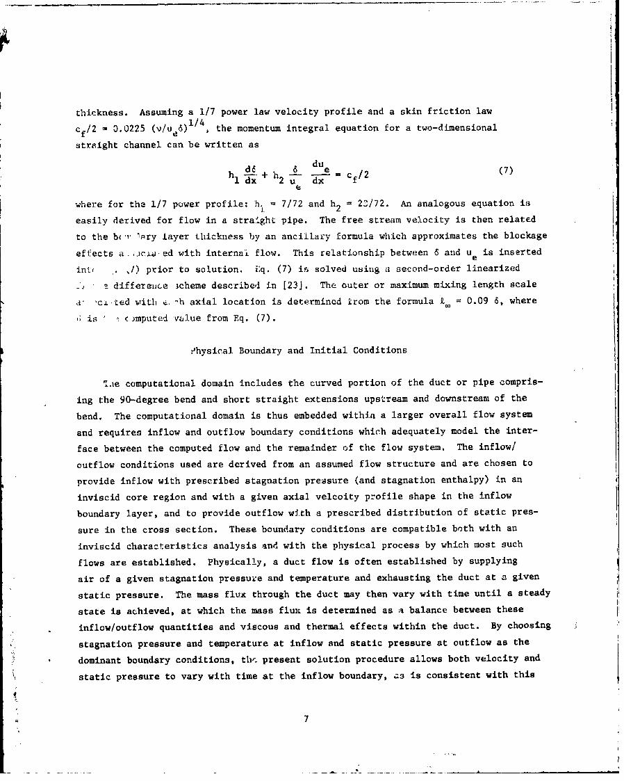
thickness. Assuming a 1/7 power law velocity profile and a skin friction law

cf/2 - 0.0225 (v/ue6) /4, the momentum integral equation for a two-dimensional

straight channel can be written as

dud6h A e /2 (7)

l dx 2 u dx Cf

where for the 1/7 power profile: h. = 7/72 and h2 22/72. An analogous equation is

easily derived for flow in a straight pipe. The free stream velocity is then related

to the b ,r' ry layer thickness by an ancillary formula which approximates the blockage

effects a. jc.a.ed with internal flow. This relationship between 6 and ue is inserted

in/) prior to solution. FEq. (7) is solved using a second-order linearized

a z difference 3cheme described in [23]. The outer or maximum mixing length scale

a' 'ct ted with e.-h axial location is determined from the formula t = 0.09 6, where

is c.nmputed value from Eq. (7).

Ahysical Boundary and Initial Conditions

lie computational domain includes the curved portion of the duct or pipe compris-

ing the 90-degree bend and short straight extensions upstream and downstream of the

bend. The computational domain is thus embedded within a larger overall flow system

and requires inflow and outflow boundary conditions which adequately model the inter-

face between the computed flow and the remainder of the flow system. The inflow/

outflow conditions used are derived from an assumed flow structure and are chosen to

provide inflow with prescribed stagnation pressure (and stagnation enthalpy) in an

inviscid core region and with a given axial velcoity profile shape in the inflow

boundary layer, and to provide outflow with a prescribed distribution of static pres-

sure in the cross section. These boundary conditions are compatible both with an

inviscid characteristics analysis and with the physical process by which most such

flows are established. Physically, a duct flow is often established by supplying

air of a given stagnation pressure and temperature and exhausting the duct at a given

static pressure. The mass flux through the duct may then vary with time until a steady

state is achieved, at which the mass flux is determined as a balance between these

inflow/outflow quantities and viscous and thermal effects within the duct. By choosing

stagnation pressure and temperature at inflow and static pressure at outflow as the

dominant boundary conditions, thr. present solution procedure allows both velocity and

static pressure to vary with time at the inflow boundary, as is consistent with this

7

physical process. As a consequence, pressure waves are transmitted upstream through

the inflow boundary during the transient flow process and are not reflected back into

the computational domain. The reflection of pressure waves at an inflow boundary

when velocity and pressure are fixed in time has often been cited as a cause of

either instability or slow convergence in other investigations. These boundary

conditions are discussed in more detail in [20]. The specific treatment of initial

and boundary conditions used here is outlined below.

The initial and boundary conditions are devised from estimates of the potential

flow velocity Ul1(X1, x 2, x3 ) for the duct, a mean boundary layer thickness 6(x1 ) for

shear layers on transverse duct or pipe walls, and finally from an estimate of the

blockage correction factor B(xI) for the core flow velocity due to the boundary layer

growth. The potential flow velocity is approximated as uniform flow in straight

segments of the duct and as Cr- 1 in curved segments. Taking C as (R0 - Ri)/£n(Ro/R.)

and d2/8[R- (R 2-d 2/4) /2] leads to a unit mass flux for rectangular and circular cross

sections, respectively. Here, Ri and R0 are the radii to the inner and outer walls

of the duct, R = (Ri + Ro)/7, and d is the pipe diameter (cf. Fig. 1). Distributions

of 6(x1 ) and B(x1 ) are determined by recourse to the simple one-dimensional momentum

integral analysis mentioned in describing the turbulence model. Finally, a shear

layer velocity profile shal- f(Y/6), o5f:l is chosen for each problem, where j is a

parameter indicative of distance from a wall. For laminar flow cases, von Karman

polynomial velocity profiles were used. For turbulent flow cases, these velocity

profile shapes were taken from the analytical fit of Musker (21] to the Coles type

of profile which matches 6 and cf from the momentum-integral calculations. The

initial values of velocity components ul, u 2, u3 are given by

Ul = UI B(x1 ) f [Y6(x 1)]

U2 =U 3 - 0

In the pipe flow calculations, estimates of the inflow radial velocity u 2 were

available and were used as initial conditions. The details of this procedure are

not critical and are omitted, since except for tho shape and thickness of the inlet

boundary layer profile, these results serve only as a convenient method for selecting

initial conditions. A reasonably accurate estimate for the pressure drop which willproduce the desired flow rate must be made using any convenient source, such as a

Moody diagram, data correlations, momentum integral analysis, or other computed

results. A smooth axial distribution of pressure which matches this pressure drop

is then assigned a,,d adjusted to approximate local curvature of the flow geometry.

8

4

This completes specification of the initial conditions. It is noted that although

these initial conditions do take into account several relevant features of the flow,

the important effects of strong secondary flows and their distortion of the primary

flow are completely neglected. The resulting inLtial flow is thus a simple but

relatively crude approximation to the final flow field.

At the inflow boundary, a "two-layer" boundary condition Is devised such that

stagnation pressure p0 is fixed in the core flow region and an axial velocity pro-

file shape ul/Ue - f(y/) is set within shear layers. Here, ue is the local edge

velocity which varies with time and is adjusted after each time step to the value

consistent with p and the local edge static pressure determined as part of the

solution. The transverse velocity components u 2 and u3 were also specified at

inf7low. For the pipe flow cases, u3 was set to zero, and the radial velozity u2

was given a smooth distribution consistent with the boundary layer thickness and

estimated axial pressure drop. For the duct flow cases, u2 and u3 were extrapolated

until the initial impulsive transients had passed and were then held fixed. The

rentining inflow condition is 92 cp /n - g (x2, x3), where n denotes the normalcoordinate direction and cp is pressure coefficient referred to reference conditions.

The quantity g is computed from the initial conditions with cp defined as l-(BU ) 2 ,

its value from the potential flow corrected for estimated ulockage. For outflow

conditions, the static pressure is impxied, and second normal derivatives cf each

ve.ocity component are set to zero. At no-slip walls, all velocity components are

set to zoro, and the remaining condition used is Dp/an = 0, where p is pressure.

The condition ;p/Dn = 0 at a no-slip surface approximates the normal momentum

equation to order Re 1 fcL viscous flow at high Reynolds number. Finally, the three-

dimensional flow cases are assumed to be symmetric about the plane containing the

curved duct centerline, and symmetry conditions are imposed on this boundary.

9

-l

SOLUTION PROCEDURE

Background

The solution procedure employs a consistently-split linearized block implicit

(LBI) algorithm which has been discussed in detail by the authors in [22,23]. There

are two important elements of this method:

(1) the use of a noniterative formal time linearization to produce

a fully-coupled linear multidimensional scheme which is written

in "block implicit" form; and

(2) solution of this linearized coupled scheme using 4 consistent

"splitting" (ADI scheme) patterned after the Douglas-Gunn 1241

(1964) treatment of scalar ADI schemes.

The method is thus referred to as a split linearized block implicit (LBI) shceme.

The method has several attributes:

(1) the noniterative linearization is efficient;

(2) the fully-coupled linearized algorithm eliminates instabilities

and/or extremely slow convergence rates often attributed to

methods which employ ad hoc decoupling and linearization

assumptions to identify nonlinear coefficients which are then

treated by lag and update techniques;

(3) the splitting or ADI technique produces an efficient algorithm

which is stable for large time steps and also provides a means

for convergence acceleration for further efficiency in computing

steady solutions;

(4) intermediate steps of the splitting are consistent with the

governing equations, and this means that the "physical" boundary

conditions can be used for the intermediate solutions. Ot':'r

splittings which are inconsistent: can have severe difficulties ii,

satisfying physical boundary conditionp [231.

(5) the convergence rate and overe" efficiency of the algorithm are

much less sensitive to mesh refinement and redistribution than

algorithms based on explicit schemes or which employ ad hoc

decoupling and linearization assumptions. This is important for

accuracy and for computing turbulent flows with viscous sublayer

resolution; and

.4 10

(6) the method is general and is specifically designed for the

complex systems of equations which govern multiscale viscous

flow in complicated geometries.

This same algorithm was later considered by Beam and Warming [25], but the ADI split-

ting was derived by approximate faetorization instead of the Douglas-Gunn procedure.

They refer to the algorithm as a "delta form" approximate factorization scheme.

This scheme replaced an earlier non-delta form scheme [26], which has inconsistent

intermediate steps.

Spatial Differencing and Artificial Dissipation

The spatial differencing procedures used are a straightforward adaption of

those used in [22] and elsewhere., Three-point central difference formulas are used

for spatial derivat,'-s, includiag the first-derivative convection and pressuregradient terms. This has an advantage over one-sided formulas in flow calculations

subject to "two-point" boundary conditions (virtually all viscous or subsonic flows),

in that all boundary conditions enter the algorithm implictly. In practical flow

calculations, artificial dissipation is usually needed and is added to control high-

frequency numerical oscillations which otherwise occur with the central-difference

fcrmula.

In the present investigation, artificial (anisotropic) dissipation terms of

the form2

S--. (8)2 2

J h 2 ax2hj xj

are added to the right-hand side of each (k-th) component of the momentum equation,

where for each coordinate direction xj, the artificial diffusivity dj is positive

and is chosen as the larger of zero and the local quantity v (a ReA -1)/Re. Here,

the local cell Reynolds number Re AX for the J-th direction is defineA by

ReAx mRe pujI Axj/Pe (9)

This treatment lowers the formal accuracy to 0 (Ax), but the functional form is such

that accuracy in representing physical shear stresses in thin shear layers with small

normal velocity is not seriously degraded. This latter property follows from the

anisotropic form of the dissipation and the combination of both small normal velocity

r 11

and small grid spacing in thin shear layers. A value of 0.5 was used for a in the

present calculations. Values lower than 0.5 have been used to good effect in two

space dimensions [27,28), but it has not yet been possible to investigate the role

of smaller a values in three space dimensions, although it is believed that lower

values of a would also be beneficial here.

Split LBI Algorithm

Linearization and Time Differencing

The system of governing equations to be solved consists of five equations:

continuity, three components of momentum and the turbulence kinetic energy equation

in five dependent variables: p, u,, u2 , u3 , and k. Using notation similar to that

in [22], at a single grid point this system of equations can be written in the

f o l w n8o m H ( O)/ at - D ( f) + S W~ (10)

where 0 is the column-vector of dependent variables, H and S are column-vector

algebraic functions of 0, and D is a column vector whose elements are the snatial

differential operators which generate all spatial derivatives appearing in the

governing equation associated with that element.

The solution procedure is based on the following two-level implicit time-

difference approximations of (10):

(Hn+l - Hn)/At .S(Dn+l + Sn+l) + (-8) (Dn +S) (11)

Hn+1 n+l n+1 nwhere, for example, H denotes H(O ) and At - t -T . The parameter B

(0.5 < 0 ý 1) permits a variable time-centering of the scheme, with a truncation

error of order [At 2, (a - 1/2) At].

A local time linearization (Taylor expansion about *n) of requisite formal

accuracy is introduced, and this serves to define a linear differential operator L

(cf. [22]) such that

Dn+l . Dn + Ln (0n+l n + 0 (At2 (12)

Similarly,

(13)Hn+l H n + (M/ao)n (0n.rl n + 0 (At2

sn+l S n + (aS/I8)n (On+l n + 0 (At2 (14)

12

Eqs. (12-14) are inserted into Eq. (II) to obtain the following system which is

linear in 0n+l

(A - BAt ,,n) (,n+. n) = At (,n + n) (15)

and which is termed a linearized block implicit (LBI) scheme. Here, A denotes a

square matrix defined by

A E (aH/ ,)n - $At (BSS/)" (16)

Eq. (15) has 0 (At) accuracy unless H *, in which case the accuracy is the same as

Eq. (11).

Special Treatment of Diffusive Terms

The time differencing of diffusive terms is modified to accomodate cross-derivative

Lerms and also turbulent viscosity and artificial dissipation coefficients which depend

on the solution variables. Although formal linearization of the convection and pres-

sure gradient terms and the resulting implicit coupiing of variables is critical to

the stability and rapid convergence of the algorithm, this does not appear to be

important for the turbulent viscosity and artificial dissipaticn coefficients. Since

the relationship between p e and d and the mean flow variables is not conveniently

linearized, these diffusive coefficients are evaluated explicitly at tn during each

time step. Notationally, this is equivalent to neglecting terms proportional to

ale /D4 or add/ao in L n, which are formally present in the Taylor expansion (12), butn nretaining all terms proportional to vt or d in both L and D

It has been found through extensive experience that this has little if any effect

on the performance of the algorithm. This treatment also has the added benefit that

the turbulence model equatiors (in this instance the turbulence kinetic energy equation)

can be decoupled from the system of mean flow equations by an appropriate matrix par-

titioning (cf. [23]) and solved separately in each step of the ADI solution procedu':e.

This reduces the block size of the block tridiagonal systems which must be solved in

each step and thus reduces the computational labor.

In addition, the viscous terms in the present formulation include a number of

spatial cross-derivative terms. Although it is possible to treat cross-derivative

terms implicitly within the ADI treatment which follows, it is not at all convenient

to do so, and consequently, all cross-derivative terms are evaluated explicitly at tn.

For a scalar model equation representing combined convection and diffusion, it has

been shown by Bema and Warming [29] that the explicit treatment of cross-derivative

terms does not degrade the unconditional stability of the present algorithm. To

13

preserve notational simplicity, it is understood that all cross-derivative terms

appearing in Ln are neglected but are retained in Dn. It is important to note that

neglecting terms in Ln has no effect on steady solutions of Eq. (15), since

P n+l-,n = 0 and thus Fq. (15) reduces to the steady form of the equations:

Dn + Sn 0 0. Aside from stability considerations, the only effect of neglecting

terms in Ln is to introduce an 0 (At) truncation error.

Consistent Srlitting of the LBI Scheme

To obtain an efficient algorithm, the linearized system (15) is split using

ADI techniques. To obtain the split scheme, the multidimensional operator L is

rewritten as the sum of three "one-dimensional" sub-operators Li (i - 1, 2, 3) each

of which contains all terms having derivatives with respect to the i-th spatial

coordinate. The split form of Eq. (15) can be derived either as in [22, 23] by

following the procedure described by Douglas and Gunn 124] in their generalization

and unification of scalar AnT cchemes, or using approximate factorization as in [25].

For the present system of equations, the split algorithm is given by

(A - OAtLn) ( * - n) . At (Dn + Sn) (17a)

(A - OAtLn) n ) - A(,* -,n) (17b)

(A - OAtL ) (0n+l_ *n) - A (0 **- n) (17c)w neo

where 4)and a) re consistent intermediate solutions [22, 12]. If spatial deriva-

tives appearing in Li and D are replaced by three-point difference formulas, as

indicated previously, then each step in Eqs. (17a-c) can be solved by a block-

cridiagrnal elimination.

Combining Eqs. (17a-c) gives

(A - BAtL n) A-1 (A - OAtLn) A-1 (A - $AtL•) (n0n+l - *n)

1 (18)

- At (Dn + Sn)

which approximates the unsplit scheme (15) to 0 (At 2). Since the intermediate steps

are also consistent approximations for Eq. (15', physical boundary conditions can be

used for 4) and 4) [22, 231. Finally, since the Li are homogeneous operators, it

follows from Eqs. (17a-c) that steady solutions have the property that 4 n+1** #nan- and satisfy

D + S 0 (19)

The steady solution thus depends only on the spatial difference approximation used

for (19) and does not depend on the solution algorithm itself.

14

COMPUTED RESULTS

Solutions for three-dimensional laminar and turbulent flow in 90-degree bends

having strong curvature and both circular and square cross sections are presented

here. To assess the degree of accuracy obtainable in this type of three-dimension•a•

flow calculation, it is obviously valuable to have experimental measurements for

comparison. Fortunately, laser-Doppler anemometry measurements have recently becont'

available [7, 8, 12, 13] for several laminar and turbulent square duct and pipe bhnth;.

Computed results for six different flow cases are included here, and the relevant flov

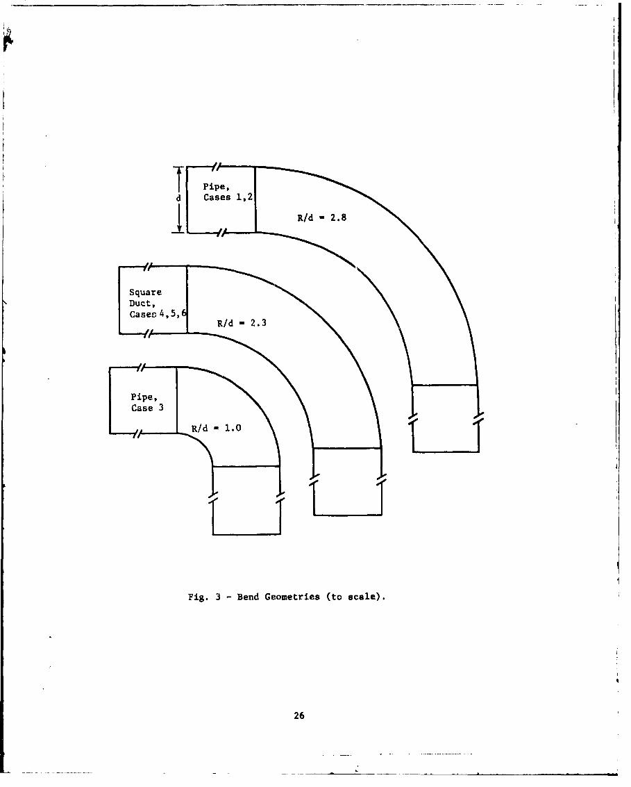
parameters describing these cases are given in Table I. Each of the three bend

geometries considered is shown to scale in Fig. 3. The cases include both laminar

and turbulent flow in a pipe bend of curvature 2.8 (cases I and 2) and in a squarc

duct of curvature 2.3 (cases 4 and 5). Measurements are given by Taylor, Whtelnw .1i

Yianneskis both for the pipe bend [13] and for the curved duct (12].

15

00

r* 0 00

0h 0- 0

x 0% 0 0%%

ON Os4 N LnPX r- C4 C 4-I N 00 00 c0o .

~ 0 00 c0 co 00 Go

0 100

9v 0 0ý 0 0D

4JU~i

00 00 M

C-C)

0 0

S. 0.

V4* 14$4 ~U 1

on Ln -4

16

The other cases include a pipe elbow configuration (Case 3), which has a curvature

of 1.0, but is otherwise identical to Case 2, and a curved duct (Case 6) which is

identical to Case 5 except that it has a nominally fully-developed inflow velocity

profile. The latter flow case was measured by Humphrey, Taylor and Whitelaw [81

and was included as one of the evaluation cases for the 1980-81 Stanford conference

on Complex Turbulent Flows.

A vast amount of information is obtained from the computation of six three-

dimensional flow cases, and only selected, representative results can be included

here. The present approachi to this problem is as follows: First, the computed

axial velocity is compared with experimental measurements in each of the five cases

!or which data is available. Next, each of the three pipe bend cases (1 - 3) is

presented in a sequence of plots designed to show the developing flow structure.

The structure of square-duct flows was consid~ered in more detail in [10, 11].

Finally, a comparison is made of the two turbulent curved duct flows which differ

only in the inflow boundary layer thickness.

Convergence Rate

Before proceeding to the discussion of computed flow behavior, an indication is

given of the degree and rate of convergence obtained in these calculations. Turbulent

flows, particularly in three dimensions, are especially difficult to compute because

of the very high degree of mesh redistribution required to resolve viscous sublayer

regions. Since peak secondary flow velocities often occur within or near the viscous

sublayer, resolution of the viscous sublayer is believed necessary to obtain an

adequate representation of the overall flow, but poses a computational problem for

which rapid convergence is difficult to achieve. The complicated flow structure in

curved ducts and pipes, which includes strong secondary flows and their resulting

distortion of the primary flow, also contributes to the difficulty of these flows.

The present computational method employs variable time steps to accelerate

convergence, as discussed in (30]. Several procedures for time step selection are

presently under evaluation, but typically small time steps are used initially during

the elimination of impulsive transients, followed by larger time steps and the ryclic

use of a sequence of time steps. In addition, a smaller time step was used near the

leading edge than elsewhere in the flow field. Small time steps are effective in

reducing high (spatial) frequency error components, while large time steps are

effective in reducing low frequency errors.

17

An indication of both the degree and rate of convergence obtained for the three-

pipe fI-w calculations (which are representative cases) is shown in Fig. 4. For

comparison, a curve representative of the convergence behavior typically obtained for

two-dimensional turbulent flow cases is also shown. Although the present convergence

rate is noticeably slower than that observed using this same algorithm in other

calculations, it is adequate for present purposes. The present calculations were

terminated as shown in Fig. 4. for reasons of economy, since it appeared that the

observed changes in the solution at this point were of minor significance and would

not alter any of the conclusions drawn from these results.

Comparison With Experiment

Computed contours of axial velocity are compared with experimental measurements

in Figs. 5 - 9. To aid in the comparison, contour values shc;,.n for the computed

solutions are the same as has been shown for the measuremtris. The computed velocities

were normalized by the mean (bulk) velocity as determined by a second-order numerical

integration of the computed solution. This calculation indicated tha t global mass

conservation was satisfied by all computed solutions to within one per cent at each

axial location. In comparing these results with the measurements, the normalized

mass flux (as evidenced by peak and centerline velocity) did not appear to match in

some cases. To aid in the comparison, the computed contours shown in Figs. 5 - 9

were renormalized to provide a nominal matching of centerline velocity at the first

measured station. Downstream stations were adjusted by this same factor. This

renormalization led to adjustment of the computed velocities by the following amounts:

Case 2 - 3.6%, Case 4 - 7.4%, Case 6 - 4%. No adjustment was required for Case 1,

and the computed mass flux was not checked for Case 5.

All of the flow cases considered here develop strong secondary flows as a result

of turning and these secondary flows result in considerable distortion of the primary

flow, particularly near the inside of the bend. This distortion of the primary flow

is the principal method of judging the agreement between measured and computed results

in Figs. 5 - 9. Both a comparison of the duct flows with two-dimensional channel flow

having the same curvature and also limited mesh refinement studies were given in a

previous study [10, l1j.

In Fig. 5, the computed results for laminar pipe flow are in 'rery good general

agreement with the measurements. The turbulent pipe flow predictions in Fig. 6 also

agree reasonably well with measurements, although the predicted flow distortion is

18

somewhat less localized than that measured. Since the laminar calculations employ

no physical assumptions beyond those of the Navier-Stokes equations, the level of

agreement is indicative of the numerical truncation error and experimental error.

The difference between the level of agreement for laminar and turbulent predictions

is at least partly an indication of error in the turbulence model. The predictions

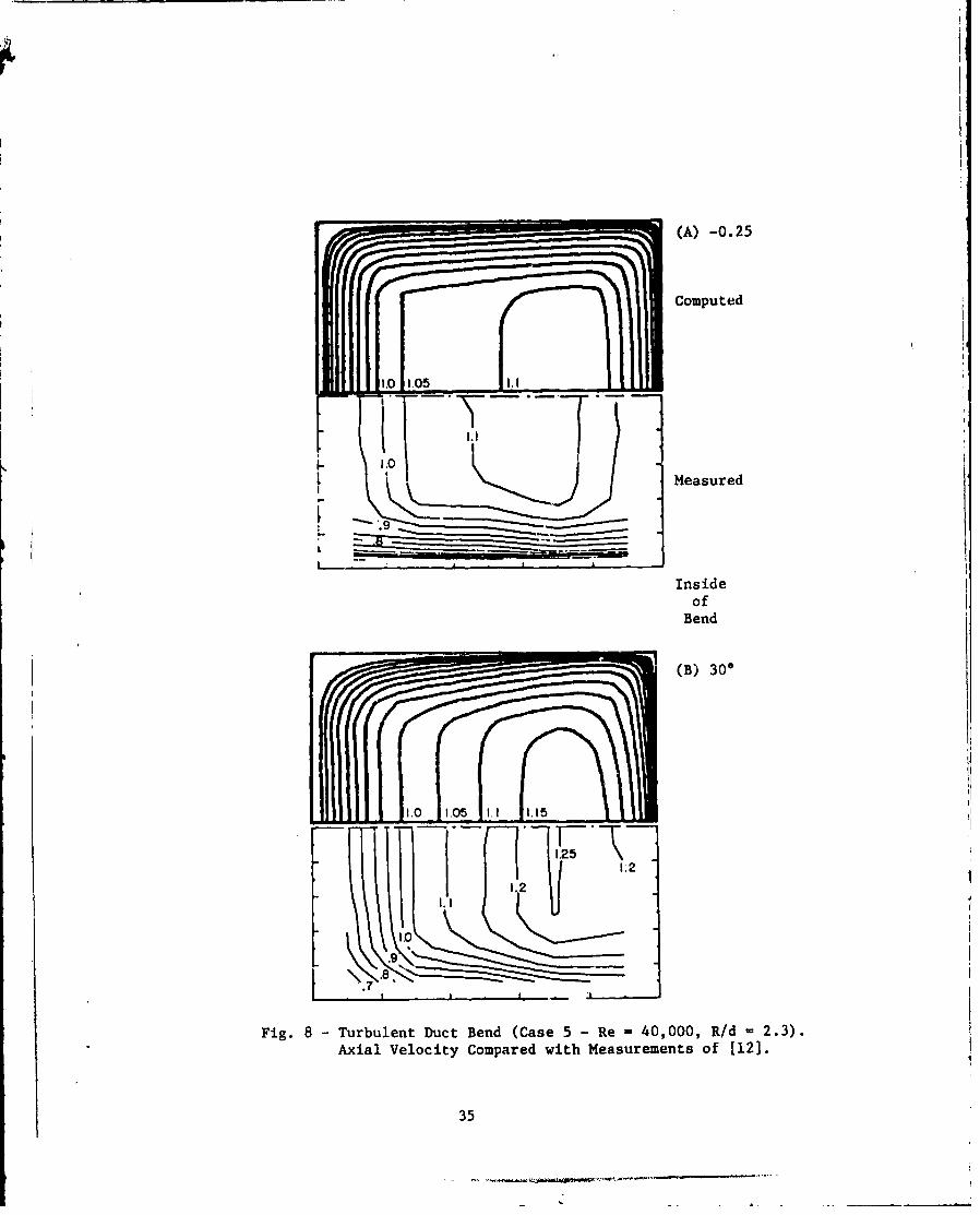
for the three duct flow cases in Figs. 7 - 9 are in good qualitative and reasonable

quantitative agreement with the measurements, although the agreement is not as good

as was obtained in the pipe flow cases. This may be partly due to the increased

difficulty of grid resolution (cf. Fig. 2) in the center of the duct, since two

grid-stretching transformations are needed for the square cross section, as opposed

to one for the circular pipe. It is also worth noting that the computed velocity

contours in Fig. 9a in the straight section 2.5 duct widths upstream of the bend

do not display the "corner distortion" found in the measurements. This distortion is

the result of weak "stress driven" secondary flows, and its absense in the computed

results is attributed to the assumption of an isotropic turbulent viscosity in the

turbulence model.

Flow Structure for Pipe Bend Cases

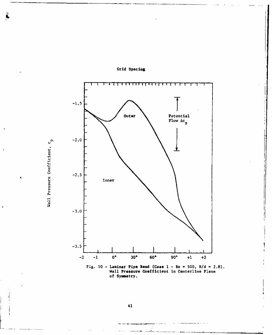
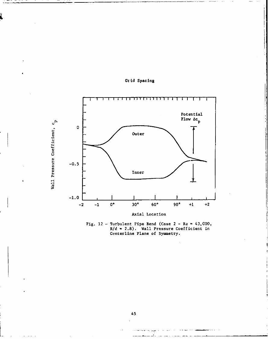
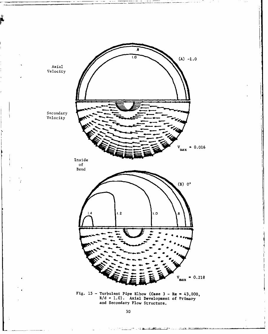
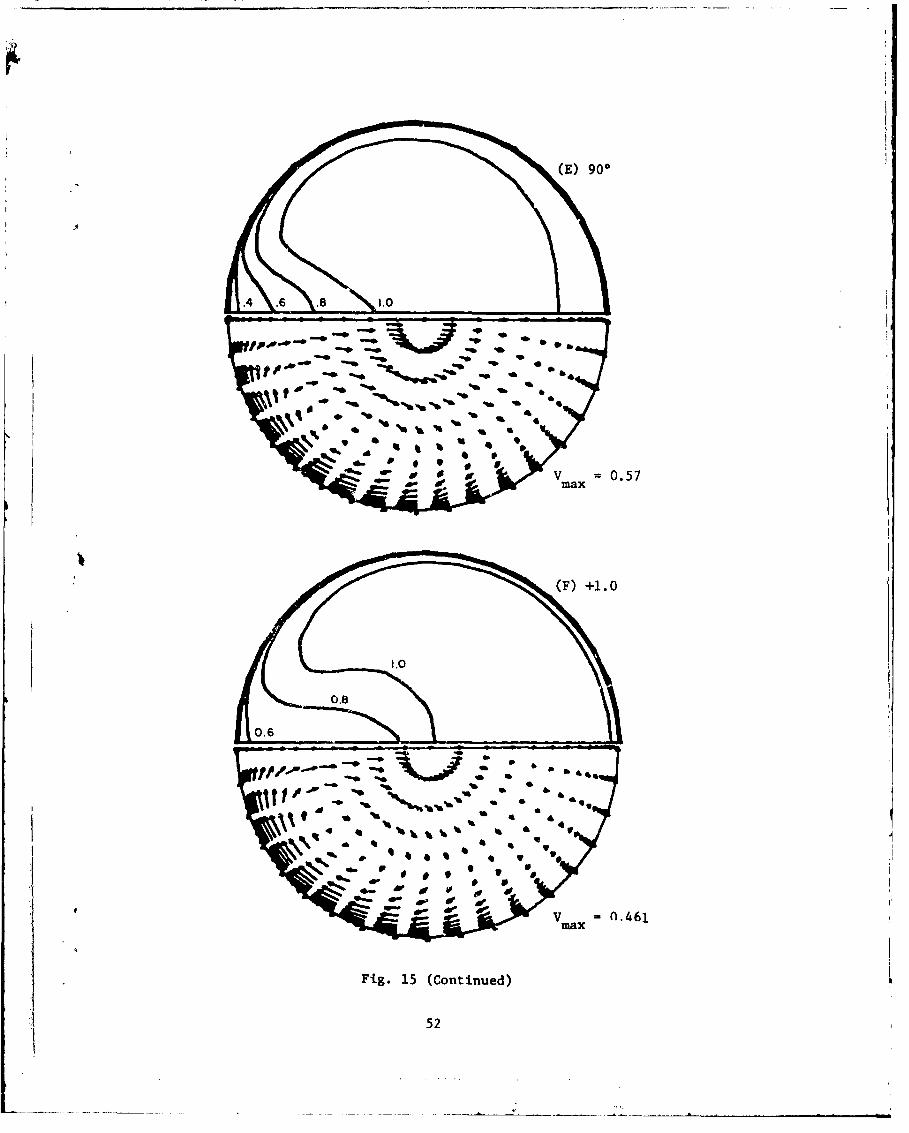
A sequence of plots is given in Figs. 10 - 15 for each of the three pipe flow

cases. These figures are designed to show the flow structure as it develops at

successive axial locations for each computed solution, the axial distribution of

pressure coefficient referred to reference conditions and bulk velocity at the inner

and outer wall locations in the plane of the centerline is first given. The pressure

coefficient provides an indication of the extent of influence of the flow in the bend

on the flow in the upstream and downstream straight extensions. The distribution of

grid points is included in these plots. Also shown is the difference in pressure

coefficient, Ac p, which would occur for a potential flow with velocity inversely

proportional to radius, in a bend of the same curvature.

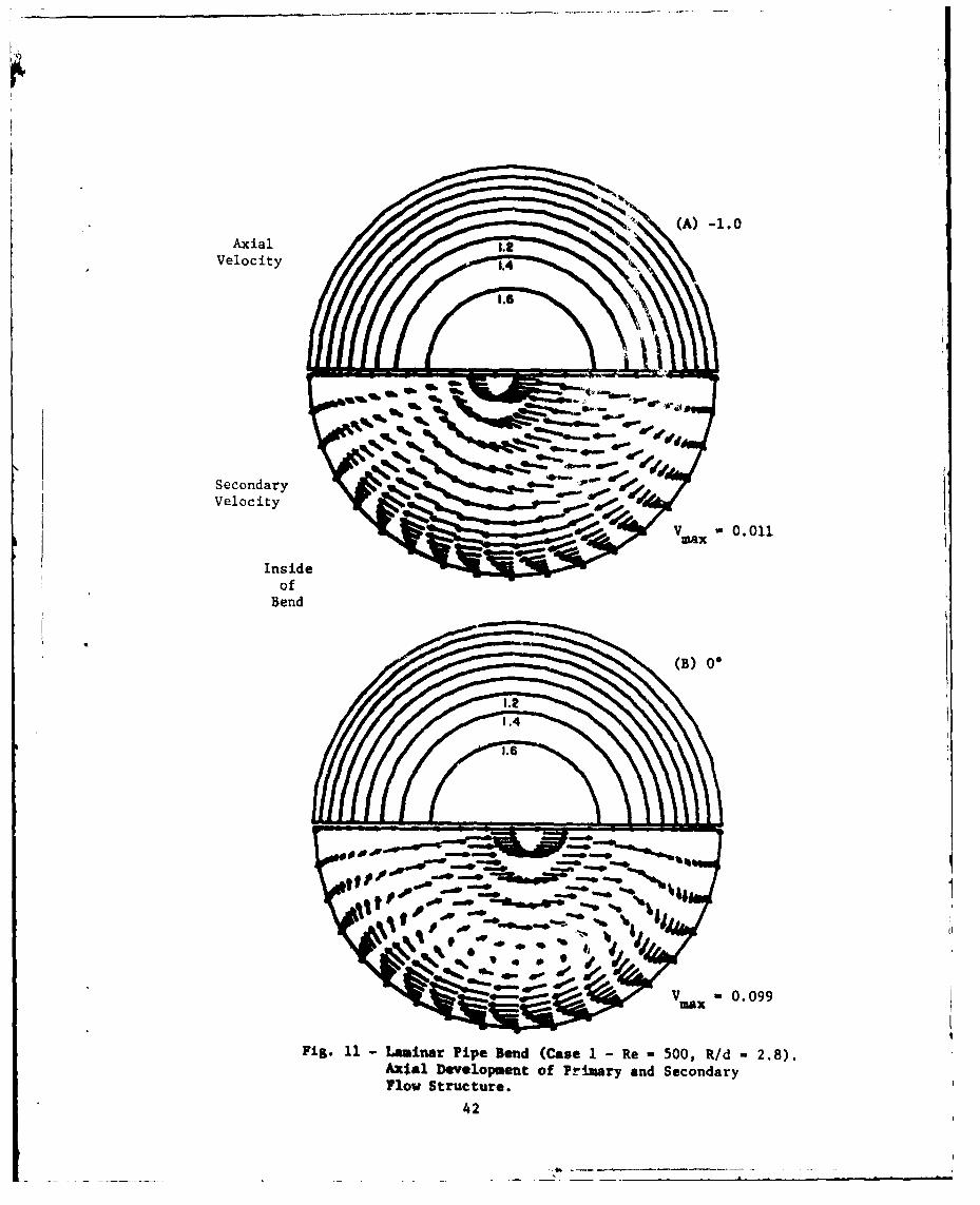
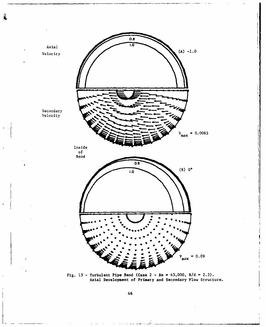
Following the pressure coefficient, a sequence showing the primary and secondary

velocity distributions at successive axial locations is given. The same contour

values are shown throughout Figs. 10 - 15; the vector magnitudes are renormalized

for each plot and thus indicate only flow direction and relative magnitude within

each plot. The strength of the secondary flows is shown by giving the magnitude of

the peak velocity-, VMAX, within the vector plot.

19

Comparing the laminar and turbulent cases in Figs. 10 -13, the laminar flow

is seen to have a mush larger pressure drop (viscous loss) and higher peak axial

velocity than the turbulent case. The secondary flows are of similar strength,

reaching about 40 per cent of the mean axial velocity. The turbulent pipe elbow

case (Figs. 14, 15) has an inflow identical to that of Case 2, but there are

considerable differences in flow development, as a result of the strong curvature.

The radial pressure gradient across the bend is very large (Fig. 14), and the

secondary velocities are over 60 per cent of the mean axial velocity. In addition,

the peak axial velocity is larger ( _- 1.6) than the 2,.3 curvature case, and occurs

near the inside of the bend rather than the outside. Somewhat surprisingly, the

only flow separation present was of very limited extent and is not visable' in the

plots. This occurred near the 90-degree location, on the inner side of the pipe

bend.

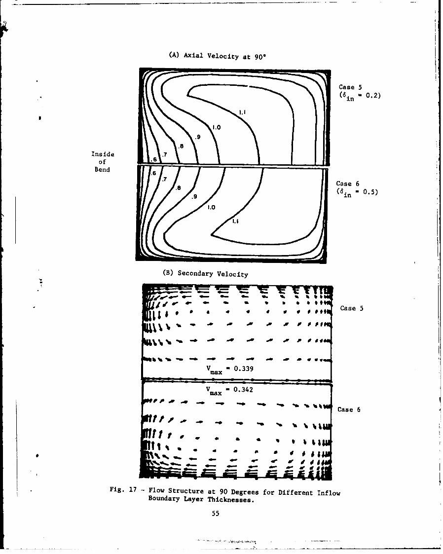
Influence of Boundary Layer Thickness on Duct Flow

The axial and secondary velocity distributions at 60 and 90 degrees are

compared in Figs. 16 - 17 for the two turbulent duct flows (cases 5, 6) with dif-

ferent inlet boundary layer thickness, 6 in' The computed flow structure is not very

sensitive to this parameter, and the most notable difference is that the distortion

of the az:ial velocity produces a thinner shear layer on the outer wall for case 6

with 6 in '0.5. Finally, the pressure coefficient for these two cases is shown in

Fig. 18. The pressure field remains largely two dimensional, although there is some

three-dimensional distortion associated with the corner '.Lrtex flow on the inside of

the bend.

20

CONCLUDING REMARKS

Three-dimensional laminar and turbulent flow within 90-degree bends of strong

curvature and both circular and square cross section has been studied by numerical

solution of the compressible Reynolds-averaged Navier-Stokes equations. Straight

extensions upstream and downstream of the bend are included in the computed flow

region. It is believed that the physical processes involved require the viscous

sublayer to be resolved, and the computational approach provides for this

resolution. Six different flow cases were considered, and the results were

evaluated by comparison with experiment measurements. In general, very good quali-

tative and reasonable quantitative agreement between solution and experiment was

observed. The developing flow structure and its dependence on geometric and flow

parameters was also studied.

Collectively, this sequence of experimeuital comparisons helps to establish

the accuracy with which these flows can be predicted by the present method using

moderately coarse grids ( ;10,000 grid points). With some allowance made for the

complexity of the flow and the difficulty of both computing and measuring flows of

this type, the agreement between computed and measured results is regarded as

generally very good. The sources of disagreement are believed attributable to

numerical truncation error and to a lesser extent the turbulence model.

21

REFERENCES

1. Hawthorne, W.R.: The Applicability of Secondary Flow Analyses to the Solutionof Internal Flow Problems, Fluid Mectanics of Internal Flow, ed. G. Sovran,(Elsevier), 1967, p. 263.

2. Hawthorne, W.R.: Research Frontiers in Fluid Dynamics, eds. R.J. Seeger andG. Temple, (Interscience), 1965, p. 1.

3. Horlock, J.H. and Lakshminarayana, B.: Secondary Flows; Theory, Experiment andApplication in Turbomachinery Aerodynamics, Annual Rev. Fluid Mech., Vol. 5,1973, p. 247.

4. Pratap, V.S. and Spalding, D.B.: Fluid Flow and Heat Transfer in Three-Dimensional Duct Flows, Int. J. Heat & Mass Transfer, Vol. 19, 1976, p. 1183.

5. Ghia, K.N. and Sokhey, J.S.: Laminar Incompressible Viscous Flow in CurvedDucts of Rectangular Cross-Sections, J. Fluid Engr., Vol. 99, 1977, p. 640.

6. Kreskovsky, J.P., Briley, W.R. and McDonald, H.: Prediction of Laminar andTurbulent Primary and Secondary Flows in Strongly Curved Ducts, NASA CR-3388,February 1981.

7. Humphrey, J.A.C., Taylor, A.M.K. and Whitelaw, J.H.: Laminar Flow in a SquareDuct of Strong Curvature, J. Fluid Mech., Vol. 83, 1977, p. 509.

8. Humphrey, J.A.C., Whitelaw, J.H. and Yee, G.: Turbulent Flow in a Square Ductwith Strong Curvature, J. Fluid Mech., 103, 443, 1981.

9. Yee, G. and Humphrey, J.A.C.: Developing Laminar Flow and Heat Transfer inStrongly Curved Ducts of Rectangular Cross-Section. ASME Paper 79-WA/HT-15,1979.

10. Buggeln, R.C., Briley, W.R. and McDonald, H.: Computation of Laminar andTurbulent Flow in Curved Ducts, Channels and Pipes Using the Navier-StokesEquations, SRA Report R80-920006-F, December 1980.

11. Buggeln, R.C., Briley, W.R. and McDonald, H.: Solution of the Navier-StokesEquations for Three-Dimensional Turbulent Flow with Viscous Sublayer Resolution.AIAA Paper No. 81-1023, 1981.

12. Taylor, A.M.K.P., Whitelaw, J.H. and Yianneskis, M.: Measurements of Laminarand Turbulent Flow in a Curved Duct with Thin Inlet Boundary Layers,Imperial College Report FS/80/29, 1980.

13. raylor, A.M.K.P., Whitelaw, J.H. and Yianneskis, M.: Curved Ducts withSecondary Motion; Velocity Measurements of Developing Laminar and TurbulentFlow (to be published in J. Fluid Engineering).

14. Hughes and Gaylord: Basic Equations of Engineering Sciace. Schaum Publishing Co.

22

1j. Roberts, G.O.: Computational Meshes for Boundary Layer Problems. Proc. 2ndInt. Conf. Num. Meth. Fluid Dynamics, (Springer-Verlag), 1971, '. 171.

16. Launder, B.E. and Spalding, D.B.: Mathematical Models of Turbulence.Academic Prcss, 1972.

17. Shamroth, S.J. and Gibeling, H.J.: The Prediction of the Turbulent Flow FieldAbout an Isolated Airfoil, AIAA Paper 79-1543, 1979. Also, NASA CR-3183, 1979.

18. Launder, B.E. and Spalding, D.B.: The Numerical Computation of Turbulent Flows.Computer Methods in Applied Mechanics and Engineering, Vol. 3, 1974, p. 269.

19. McDonald, H. and Fish, R.W.: Practical Calculations of Transitional BoundaryLayers. International Journal of Heat and Mass Transfer, Vol. 16, No. 9,1973, pp. 1729-1744.

20. McDonald, H. and Briley, W.R.: Some Observations on Numerical Solutions ofthe Three-Dimensional Navier-Stokes Equations. Symposium on Numerical andPhysical Aspects of Aerodynamic Flows. Cal. State Univ. (Long Beach), 1981.

21. Musker, A.J.: Explicit Expression for the Smooth Wall Velocity Distribution

in a Turbulent Boundary Layer. AIAA Journal, Vol. 17, 1979, p. 655.

22. Briley, W.R. and McDonald, H.: Solution of the Multidimensional Compressible

Navier-Stokes Equations by a Generalized Implicit Method. J. of Comp. Physics,Vol. 234, Aug. 1977, p. 372.

23. Briley, W.R. and McDonald, 1E.: On the Structure and Use of Linearized BlockADI ant Related Schemes. J. Comp. Physics, Vol. 34, 1980, p. 54.

24. Douglas, J. and Gunn, J.E.: A General Formulation of Alternating DirectionMethods. Numerische Math., Vol. 6, lq 6 4, p. A28.

25. Beam, R.M. and Warming, R.F.: An Implicit Factored Scheme for the CompressibleNavier-Stokes Equations. AIAA Journal, Vol. 16, April 1978, p. 393.

26. Beam, R.M. and Warming, R.F.: An Implicit Finite-Difference Algorithm forHyperbolic Systems in Conservation Law Form. Journal of Computational Physics,Vol. 22, Sept. 1976, p. 87.

27. Shamroth, S.J., McDo id, H. and Briley, W.R.: A Navier-Stokes Solution forTransonic Flow Throtbh a Cascade. SRA Report R79-920007-F, 1979.

28. McDonald, H., Shamroth, S.J. and Briley, W.R.: Transonic Wlows with ViscousEffects. Transonic Shock and Multidimensional Flows: Advances in ScientificComputing. R.E. Meyer, Ed., Academic Press, New York, 1982.

29. Beam, R.M. and Warming, R.F.: Alternating Direction Implicit Methods forParabolic Equations with a Mixed Derivative. SIAM J. Sci. Stat. Comp.,Vol. 1, 1980, p. 131.

30. McDonald, H. and Briley, W.R.: Computational Fluid Dynamic Aspects of InternalFlows. AIAA Paper No. 79-1445, 1979.

23

x2

Ri x3

4~x3

R____ R r-R

(a) Plane of Centerline (b) Plane Normal toCurvature Centerline

Fig. 1 - Schematic of Coordinate System.

24

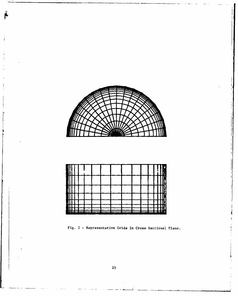
IHl I

Fig. 2 - Representative Grids in Cross Sectional Plane.

25

T Pipe,

F C3ses 1, Gmr ( sl[ , _ R/d 2.8 "

Square

Duct,Cases, 4, 5,( =

Pipe,

Case 3

Fig. 3 -Bend Geometries (to scale).

26

107

3

Pipe Bend

10

103

0 100

Number of Iterations

Fig. 4 -Convergence Rate for Selected Cases.

27

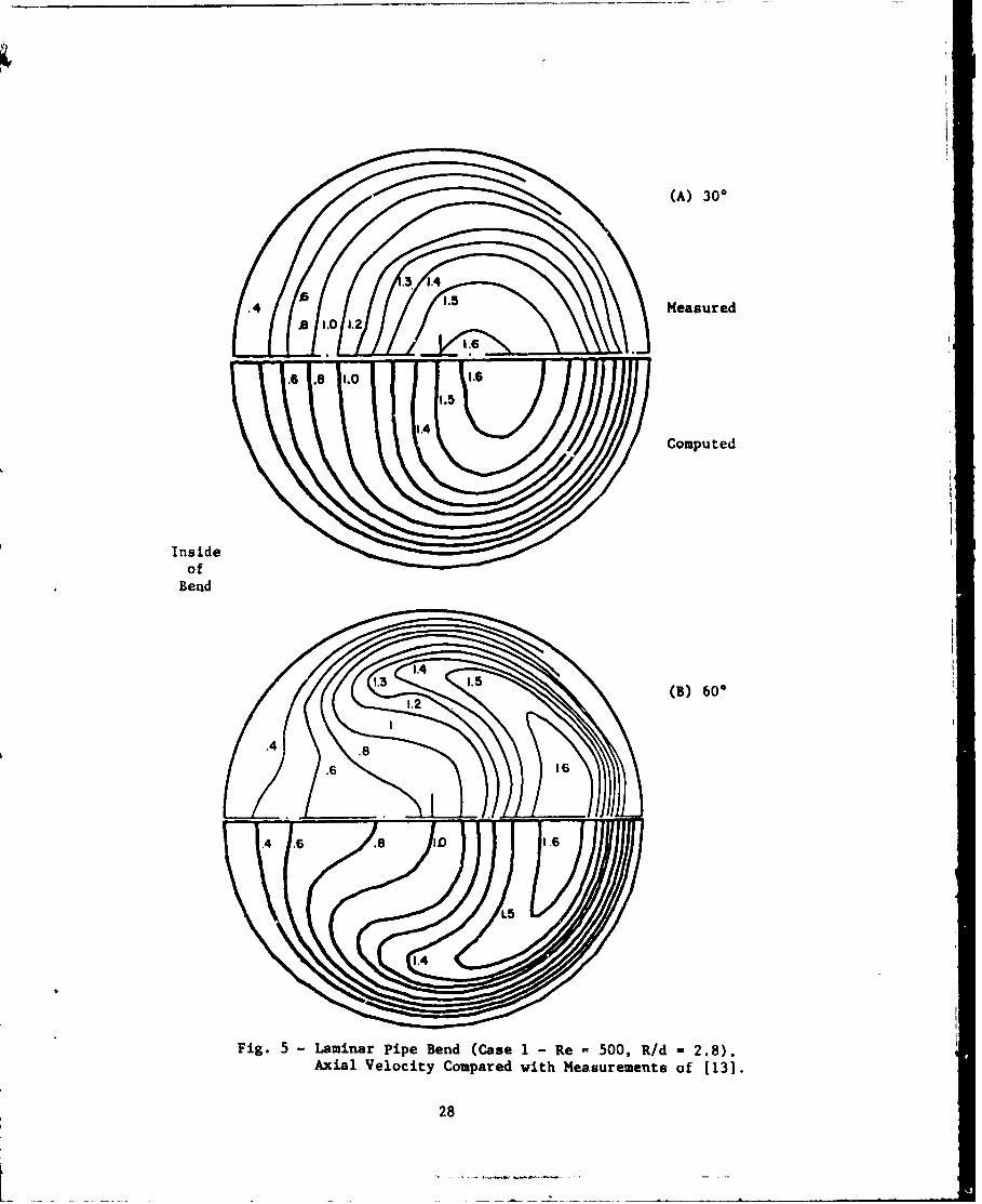
(A) 300

.4 z 1.5Measured

Computed

Insideof

Benid

(B) 600

128

1.2 Cc) 750

(D.01.

.4.

1.29

(A) 30*

6 Measured

1.2 1.1 1.0 .9 .8 S

Computed

Insideof

Bend

(B) 60*

Fig. 6 - Turbulent Pipe Bend (case 2 - Re -43,000,Rid - 2.8). Axial Velocity Compared withMeasurements of [131.

30

(C) 75-

.8.9 1.0 1.1

.........

1.15 (D) + 1.0

Fig. 6 (Continued)

31

(A) -0. 25

Computed

1.4 Measured

Insideof

Bend

(B) 300

Fig. 7 -Laminar Duct Bend (Case 4 -Re -790, R/d 2.3).Axial Velocity Compared with measurements of [121.

32

'p71.5

'1.6

S(D) 77.50

..8\ .61.4 -.

Fig. 7 (Continued)

33

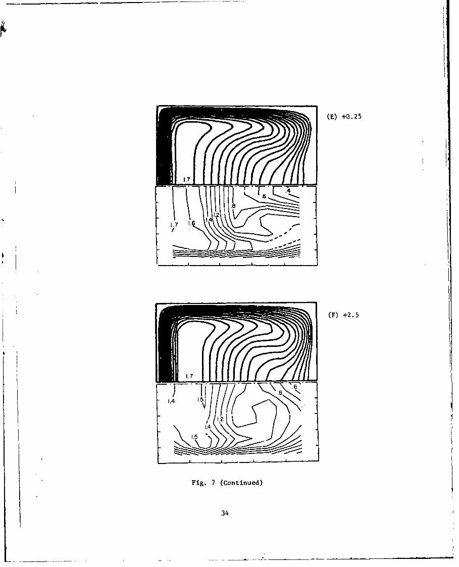
(E) +0.25

1.7

/ . 61

S12

_1..

(F) +2.5

1.7[4.8 6

'K-

Fig. 7 (Continued)

34

(A) -0.25

Computed

1.0 5 _ _ II , _. _

9 Measured

Inside

ofBend

(B) 30'

..7 .8

Fig. 8 - Turbulent Duct Bend (Case 5 - Re - 40,000, R/d - 2.3).Axial Velocity Compared with Measurements of [12].

35

(C) 600

10 1.05 1.1

r I I ,,III.• .

(D) 77.50

10 1.05

• I ,

Fig. 8 (Continued)

36

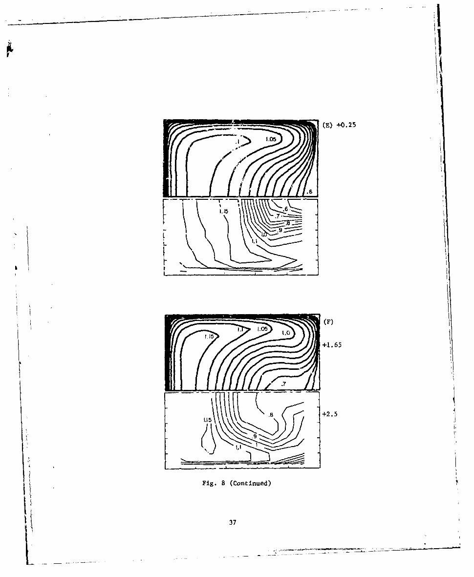
(E) +0.25

J= • " ==='•t. 1.0 5

iL1.65

1 .15 '

I. Fig. 8 (Continued)

S37

Insidef

(A) -2.5Bend ..0

1.2

Measured Computed

Outside (B) O0

ofBend

.3.2

1.2 1.22

Fig. 9 - Turbulent Duct Bend (Case 6 - Re - 40,000, R/d 2.3).Axial Velocity Compared with Measurements of [8].

38

(C) 450

Fi. 2 (Cntnud

399

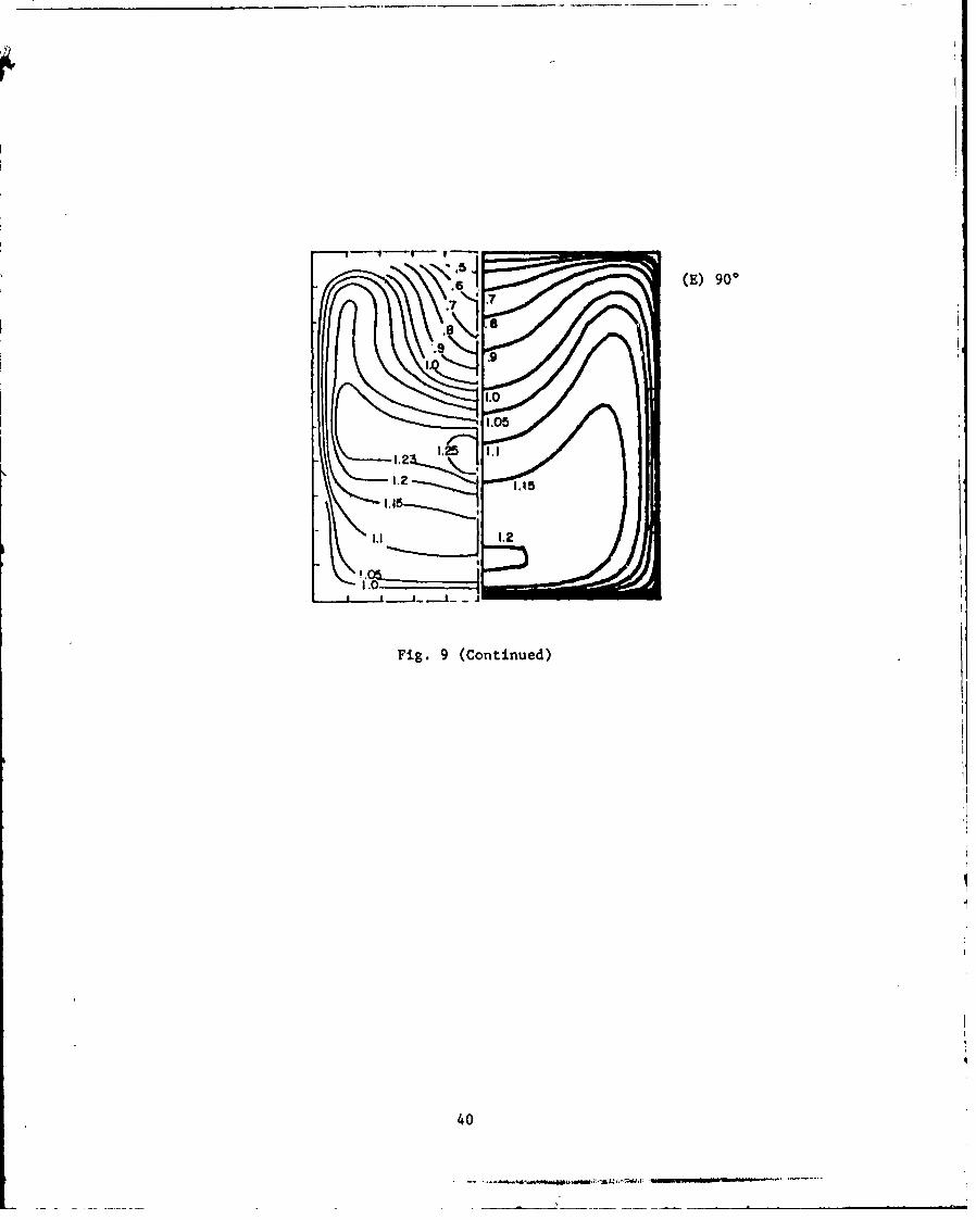
"(E) 900

I.8

I..9

Fig. 9 (Continued)

40

Grid Spacint

-1,5

OutotrntialFlow Ac.

p

-2.0

U

4.J

S-2.5

SInner

aJ

P-4

:3:

-3.0

-3.5 I

-2 -1 00 30* 60* 901 +1 +2

Fig. 10 - Laminar Pipe Bend (Case I - Re - 500, R/d - 2.8).Wall Pressure Coefficient in Centerline Planeof Symmetry.

41

AxialVelocity1.

Velocity

Insideof

Bend

~(B 0*0

Owl%. Devlomet WOf Vrmr and Secodar

Flow Structure.

42

(C) 30*

II

Naa

143

.6 .8 12hC6 .6

7;, 00V .0 0.19

a v ~~max 0 9

1.4e

1.0

dd 00 6

A.,

Fig. 11 (Continued)

44

Grid Spacing

~~I I i I I I'IIII II I I I II IIII I I1 I 11

Potential0 Flow AcU p

o Outer

U

S~Inner

r-4

-1.0

-2 -1 0 30* 600 900 +1 +2

Axial Location

Fig. 12 -Turbulent ripe Bend (Case 2 - Re -43,000,R/d - 2.8). Wall Pressure Coefficient inCenterline Plane of Symmetry.

45

Axial

Velocity

Secondary 6~

Velocity \'~~~q~iZ

of

Ben

b V

W

Fig. 13 -Turbulent Pipe Bend (Case 2 -Re --43,000, R/d 2.3).Axial Development of Primary and Secondary Flow Structure.

46

tow

a~ _ a

4I

d .7

& w

.4b

900

-- 3

0 &

lb 4

V 0.215max

Fi. 13(Cn.nud

48 4

Grid Spacing

I I I I I !I IlIIIlIll~ll I I I I ... I' I ' I -

1.0Potential

Flow AcOuter

0

U -1.0

1JInner

U.44

0 -2.0U

U)

$4

-3.0 I I I I-2 - 0 900 +1 +2 +3 +4 +5

Axial Location

Fig. 14 - Turbulent Pipe Elbow (Case 3 - Re 43,000,R/d = 1.0). Wall Pressure Coefficient inCenterline Plane of Symmetry.

49

AxialVelocity

Sec ondary- -Velocity ~ *

of

R/d4 1.0) Axia Deeomn 8o rmr

506

dV n. ''

-(C) 30

1.6 1.41.2 1.0.8 .

510.1

4-

Ar max

44

Fig. 15 (Continued)

52

I..

Fig. 15 (Continued)

53

(A) Axial Velocity at 600

Case 5(6 in -0.2)

Inside 1110 9.of -

B end 1110 .

Case 6( 6 in -0.5)

(B) Secondary Velocity

0- d6 0 Caztse 5

W.u av W. -w a. 4 ad~e

psV mx=0.428

max Casue 6

"" qk_ a 0'a d

Fig. 16 - 'Flow Structure at 60 Degrees for Different

Inf low Boundary Layer Thicknesses.

(A) Axial Velocity at 90o

Case 5(6i 0.2)

.8Inside

Bend .

.7 Case 6.9 (6 in 0.5)

I.0

1.1

(B) Secondary Velocity

Case 5

V 0.339

Vmax 0.342

~P ' - -Case 6

1k,.. - ~ d.

Fig. 17 -Flow Structure at 90 Degrees for Different Inf lowBoundary Layer Thicknesses.

55

(A) Pressure Coefficient at 600

-.6 Case 5(6i 0.2)

.7

-. 6 -. 5 -.A -.3 -.2 -1 0 .1 __

-. 6 .5 -4 -3 -. -.1 0 2 Case 6(6 in 0.5)

(B) Pressure Coefficient at 900

5 ~Case 5

- -2 -0

-. 4-.-.

Case 6

Fig. 18 -Pressure Coefficient for Different

Inlet Boundary Layer Thicknesses.

56

DISTRIBUTION LIST (Continued)Page Eight

Professor J.F. Thompson Dr. S. BeusMississippi State University Bettis Atomic Power LaboratoryDepartment of Aerophysics and P.O. Box 79

Aerospace Engineering West Mifflin, PA 15122State College, MS. 39762

Mr. M. Lubert

AFDRD-AS/M General Electric CompanyU.S. Air Force Knolls Atomic Power Laboratory

The Pentagon P.O. Box 1072Washington, DC 20330 Schnectady, NY 12301

Air Force Office of ScientificResearch/NA

Building 410Bolling AFBWashington, DC 20332

Naval Air Systems CommandCode 03Washington, DC 20361

Naval Air Systems CommandCode 03BWashington, DC 20361

Naval Air Systems CommandCode 310Washington, DC 20361

Mr. Raymond F. SiewertNaval Air Systems CommandCode 320DWashington, DC 20361

Naval Air Systems CommandCode 5301Washington, DC 2036]

Mr. Robert J. HansenNaval Research LaboratoryCode 8441Washington, DC 20375

Mr. Walter EngleNaval Sea Systems CommandCode 08Washington, DC 20362

DISTRIBUTION LIST (Continued)Page Seven

Professor Ronald W. Yeung Mr. John L. HessMassachusetts Institute of Technology Douglas Aircraft CompanyDepartment of Ocean Engineering 3855 Lakewood BoulevardCambridge, MA 02139 Long Beach, CA 90801

Professor Allen Plotkin Dr. H.K. ChengUniversity of Maryland University of Southern CaliforniaDepartment of Aerospace Engineering University ParkCollege Park, MD 20742 Department of Aerospace Engineering

Los Angeles, CA 90007Professor J.M. Burgers

University of Maryland Professor J.J. StokerInstitute of Fluid Dynamics New York University

and Applied Mathematics Courant Institute ofCollege Park, MD 20742 Mathematical Sciences

251 Mercer StreetDr. Robert K.-C. Chan New York, NY 10003JAYCOR1.401 Camino Del Mar Librarian, Aeronautical LaboratoryDel Mar, CA 92014 National Research Council

Montreal RoadDr. Robert H. Kraichnan Ottawa 7, CanadaDublin, NH 03444

Professor Norman J. ZabuskyMr. Dennis Bushnell University of PittsburghNASA-Langley Research Center Department of MathematicsLangley Station and StatisticsHampton, VA 23365 Pittsburgh, PA 15260

Techiical Library Technical LibraryNaval Ordnance Station Naval Missile CenterIndian Head, MD 20640 Point Mugu, CA 93041

Professor S.F. Shen Dr. Harvey SegurCornell University Aeronautical Research AssociatesSibley School of Mechanical of Princeton, Inc.

and Aerospace Engineering 50 Washington RoadIthaca, NY 14853 Princeton, NJ 08540

Mr. Marshall P. Tulin Professor S.I. ChengHydronautics, Incorporated Princeton University7210 Pindell School Department of Aerospace andLaurel, MD 20810 Mechanical Sciences

The Engineering QuadrangleDr. J.C.W. Rogers Princeton, NJ 08540The Johns Hopkins UniversityApplied Physics Laboratory Dr. T.F. ZienJohns HopkilLs Road Naval Surface Weapons CenterLaurel, MD 20810 White Oak Laboratory

Room 427-544Silver Spring, MD 20910

DISTRIBUTION LIST (Continued)Page Six

Dr. Gary Chapman Dr. Nils SalvesenAmes Research Center David W. Taylor Naval Ship ResearchMail Stop 227-4 and Development CenterMoffett Field, CA 94035 Code 1552

Bethesda, MD 20084

Deputy DirectorTactical Technology Office Mrs. Joanna W. SchotDefense Advanced Research David W. Taylor Naval Ship Research

Projects Agency and Development Center1400 Wilson Boulevard Code 1843Arlington, VA 22209 Bethesda, MD 20084

Professor Alexandre J. Chorin Dr. George R. IngerUniversity of California Virginia Polytechnic InstituteCenter for Pure and Applied Mathematics and State University

Berkeley, CA 94720 Department of Aerospace andOcean Engineering

Professor Joseph L. Hammack, Jr. Blacksburg, VA 24061University of CaliforniaDepartment of Civil Engineering Dr. Ali H. NayfehBerkeley, CA 94720 Virginia Polytechnic Institute

and State UniversityProfessor Paul Lieber Department of Engineering MechanicsUniversity of California Blacksburg, VA 24061Department of Mechanical EngineeringBerkeley, CA 94720 Professor C. C. Mei

Massachusetts Institute of TechnologyDr. Harvey R. Chaplin, Jr. Department of Civil EngineeringDavid W. Taylor Naval Ship Research Cambridge, MA 02139

and Development CenterCode 1600 Professor David J. BenneyBethesda, MD 20084 Massachusetts Institute of Technology

Department of MathematicsDr. Francois N. Frenkiel Cambridge, MA 02139David W. Taylor Naval Ship Research

and Development Center Professor Phillip MandelCode 1802.2 Massachusetts Insitute of TechnologyBethesda, MD 20084 Department of Ocean Engineering

Cambridge, MA 02139

Mr. G'.ne H. Gleissner

David W. Taylor Naval Ship Research Professor J. Nicholas Newmanand Development Center Massachusetts Institute of Technology

Code 1800 Department of Ocean EngineeringBethesda, MD 20084 Room 5-324A

Cambridge, MA 02139Dr. Pao C. PienDavid W. Taylor Naval Ship Research Professor Francis Noblesse

and Development Center Masachusetts Institute of TechnologyCode 1521 Department of Ocean EngineeringBethesda, MD 20084 Cambridge, MA 02139

DISTRIBUTION LIST (Continued)Page Five

Professor L. Gary Leal Dr. Jack W. HoytCalifornia Insitute of Technology Naval Ocean Systems CenterDivision of Chemistry and Chemical Engineering Code 2591Pasadena, CA 91125 San Diego, CA 92152

Professor H.W. Liepmann Professor Richard L. PfefferCalifornia Insitute of Technology Florida State UniversityGraduate Aeronautical Laboratories Geophysical Fluid Dynamics InstitutePasadena, CA 91125 Tallahassee, FL 32306

Professor A. Roshko Dr. Denny R.S. KoCalifornia Institute of Technology Dynamics Technology, Inc.Graduate Aeronautical Laboratories 22939 Hawthorne Boulevard, Suite 200Pasadena, CA 91125 Torrance, CA 90505

Dr. Leslie M. Mack Professor Thomas J. HanrattyJet Propulsion Laboratory University of Illinois atCalifornia Institute of Technology Urbana-ChampaignPasadena, CA 91103 Department of Chemical Engineering

205 Roger Adams LaboratoryProfessor K.M. Agrawal Urbana, IL 61801Virginia State CollegeDepartment of Mathematics Air Force Office of ScientificPetersburg, VA 23803 Research/NA

Building 410Technical Library Balling AFBNaval Missile Center Washington, DC 20332Point Mugu, CA 93041

Professor Hsien-Ping PaoProfessor Francis R. Hama The Catholic University of AmericaPrinceton University Department of Civil EngineeringDepartment of Mechanical and Washington, DC 20064

Aerospace EngineeringPrinceton, NJ 08540 Dr. Phillip S. Klebanoff

National Bureau of StandardsDr. Joseph H. Clarke Mechanics SectionBrown University Washington, DC 20234Division of EngineeringProvidence, RI 02912 Dr. G. Kulin

National Bureau of StandardsProfessor J.T.C. Liu Mechanics SectionBrown University Washington, DC 20234Division of EngineeringProvidence, RI 02912 Dr. J.0. Elliot

Naval Research LaboratoryChief, Document Section Code 8310Redstone Scientific Information Center Washington, DC 20375Army Missile CommandRedstone Arsenal, AL 35809 Mr. R.J. Hansen

Naval Research LaboratoryCode 8441Washington, DC 20375

DISTRIBUTION LIST (Continued)Page Four

Professor S.I. Pai Mr. Steven A. OrszagUniversity of Maryland Cambridge Hydrodynamics, Inc.Institute of Fluid Dynamics 54 Baskin Road

and Applied Mathe•-tics Lexington, MA 02173College Park, MD -20742

Professor Tuncer CebeciComputation and Analyses Laboratory California State UniversityNaval Surface Weapons Center Mechanical Engineering DepartmentDahlgren Laboratory Long Beach, CA 90840Dahlgren, VA 22418

Dr. C.W. HirtDr. Robert H. Kraichnan University of CaliforniaDublin, NH 03444 Los Alamos Scientific Laboratory

P.O. Box 1663Professor Robert E. Falco Los Alamos, NM 87544Michigan State UniversityDepartment of Mechanical Engineering Professor Frederick K. BrowandEast Lansing, MI 48824 University of Southern California

University ParkProfessor E. Rune Lindgren Department of Aerospace EngineeringUniversity of Florida Los Angeles, CA 90007Department of Engineering Sciences231 Aerospace Engineering Building Professor John LauferGainesville, FL 32611 University of Southern California

University ParkMr. Dennis Bushnell Department of Aerospace EngineeringNASA Langley Research Center Los Angeles, CA 90007Langely StationHampton, VA 23365 Professor T.R. Thomas

Teesside PolytechnicDr. A.K.M. Fazle Hussain Department of Mechanical EngineeringUniversity of Houstci Middlesbrough TSI 3BA, ENGLANDDepartment of Mechanical EngineeringHouston, TX 77004 Dr. Arthur B. Metzner

University of DelawareProfessor John L. Lumley Department of Chemical EngineeringCornell University Newark, DE 19711Sibley School of Mechanical

and Aerospace Engineering Professor Harry E. RauchIthaca, NY 14853 The Graduate School and University

Center of the City UniversityProfessor K.E. Shuler of New YorkUniversity of California, San Diego Graduate Center: 33 West 42 StreetDepartment of Chemistry New York, NY 10036La Jolla, CA 92093

Mr. Norman M. NilsenDr. E.W. Montroll Dyntec CompanyPhysical Dynamics, Inc. 5301 Laurel Canyon Blvd., Suite 201P.O. Box 556 North Hollywood, CA 91607La Jolla, CA 92038

DISTRIBUTION LIST (Continued)Page Three

Librarian Station 5-2 Dr. Charles Watkins, HeadCoast Guard Headquarters Mechanical Engineering DepartmentNASSIF Building Howard University400 Seventh Street, SW Washington, DC 20059Washington, DC 20591

Professor W.W. WillmarthLibrary of Congress The University of MichiganScience and Technology Division Department of Aerospace EngineeringWashington, DC 20540 Ann Arbor, MI 48109

Dr. A.L. Slafkosky Office of Naval ResearchScientific Advisor Code 481Commandant of the Marine Corps 800 N. Quincy StreetCode AX Arlington, VA 22217Washington, DC 20380

Professor Richard W. MiksadMaritime Administration The University of Texas at AustinOffice of Maritime Technology Department of Civil Engineering14th & E Streets, NW Austin, TX 78712Washington, DC 20230

Professor Stanley CorrsinMaritime Administration The Johns Hopkins UniversityDivision of Naval Architecture Department of Mechanics and14th & E Streets, NW Materials SciencesWashington, DC 20230 Baltimore, MD 21218

Dr. G. Kulin Professor Paul LieberNational Bureau of Standards University of CaliforniaMechanics Section Department of Mechanical EngineeringWashington, DC 20234 Berkeley, CA 94720

Naval Research Laboratory Professor P.S. VirkCode 2627 Massachusetts Institute of TechnologyWashington, DC 20375 6 copies Department of Chemical Engineering

Cambridge, MA 02139LibraryNaval Sea Systems Command Professor E. Mollo-ChristensenCode 09GS Massachusetts Institute of TechnologyWashington, DC 20362 Department of Meteorology

Room 54-1722Mr. Thomas E. Peirce Cambridge, MA 02139Naval Sea Systems CommandCode 03512 Professor Patrick LeeheyWashington, DC 20362 Massachusetts Institute of Technology

Department of Ocean EngineeringMr. Stanley W. Doroff Cambridge, MA 02139Mechanical Technology, Inc.2731 Prosperity Avenue Professor Eli ReshotkoFairfax, VA 22031 Case Western Reserve University

Department of Mechanical andAerospace Engineering

Cleveland, OH 44106

DISTRIBUTION LIST (Continued)Page Two

Library The Society of Naval Architects and

Naval Weapons Center Marine EngineersChina Lake, CA 93555 One World Trade Center, Suite 1369

New York, NY 10048Technical LibraryNaval Surface Weapons Center Technical LibraryDahlgren Labcratory Naval Coastal System Laboratory

Dahlgren, VA 22418 Panama City, FL 32401

Technical Documents Center Professor Theodore Y. Wu

Army Mobility Equipment Research Center California Insitute of Technology

Building 315 Engineering Science Department

Fort 13elvoir, VA 22060 Pasadena, CA 91125

Technical Library DirectorWebb Institute of Naval Architecture Office of Naval Research Western

Glen Cove, NY 11542 Regional Office1030 E. Green Street

Dr. J.P. Breslin Pasadena, CA 91101Stevens Institute of TechnologyDavidson Laboratory Technical Library

Castle Point Station Naval Ship Engineering CenterHoboken, NJ 07030 Philadelphia Division

Philadelphia, PA 19112

Professor Louis LandweberThe Univcrsity of Iowa Army Research OfficeInstitute of Hydraulic Research P.O. Box 12211Iowa City, IA 52242 Research Triangle Park, NC 27709

R.E. Gibson Library EditorThe Johns Hopkins University Applied Mechanics ReviewApplied Physics Laboratory Southwest Research InstituteJohns Hopkins Road 8500 Culebra RoadLaurel, MD 20810 San Antonio, TX 78206

Lorenz G. Straub Library Technical LibraryUniversity of Minnesota Naval Ocean Systems CenterSt. Anthony Falls Hydraulic Laboratory San Diego, CA 92152Minneapolis, MN 55414

ONR Scientific Liaison GroupLibrary American Embassy - Room A-407Naval Postgraduate School APO San Francisco 96503Monterey, CA 93940

LibrarianTechnical Library Naval Surface Weapons CenterNaval Underwater Systems Center White Oak LaboratoryNewport, RI 02840 Silver Spring, MD 20910

Engineering Societies Library Defense Research and Development Attache345 East 47th Street Australian EmbassyNew York, NY 10017 1601 Massachusetts Avenue, NW

Washington, DC 20036

DISTRIBUTION LIST FOR UNCLASSIFIEDTECHNICAL REPORTS AND REPRINTS ISSUED UNDER

CONTRACT NOOO14-81-C-0377 TASK 062-648

All addressees receive one copy unless otherwise specified

Defense Technical Information Center NASA Scientific and TechnicalCameron Station Information FacilityAlexandria, VA 22314 12 copies P.O. Box 8757

Baltimore/WashingtonProfessor Bruce Johnson International AirportU.S. Naval Acaderay Maryland, 21240Engineering DepartmentAnnapolis, MD 21402 Professor Paul M. Naghdi

University of CaliforniaLibrary Department of Mechanical EngineeringU.S. Naval Academy Berkeley, CA 94720Annapolis, MD 21402

LibrarianTechnical Library University of CaliforniaDavid W. Taylor Naval Ship Research Department of Naval Architecture

and Development Center Berkeley, CA 94720Annapolis LaboratoryAnnapolis, MD 21402 Professor John V. Wehausen

University of CaliforniaProfessor C.-S. Yih Department of Naval ArchitectureThe Universit~y of Michigan Berkeley, CA 94720Department of Engineering MechanicsAnn Arbor, MI 48109 Library

David W. Taylor Naval Ship ResearchProfessor T. Francis Ogilvie and Development CenterThe University of Michigan Code 522.1Department of Naval Architecture Bethesda, ND 20084

and Marine EngineeringAnn Arbor, MI 48109 Mr. Justin H. McCarthy, Jr.

David W. Taylor Naval Ship ResearchOffice of Naval Research and Development CenterCode 200B Code 1552800 N. Quincy Street Bethesda, MD 20084Arlington, VA 22217 3 copies

Dr. William B. MorganOffice of Naval Research David W. Taylor Naval Ship ResearchCode 438 and Development Center800 N. Quincy Street Code 1540Arlington, VA 22217 Bethesda, MD 20084

Of fice of Naval Research DirectorCode 473 Office of Naval Research Eastern/Central800 N. Quincy Street Building 114, Section D -Regional OfficeArlington, VA 22217 666 Slimmer Street

Boston, MA 02210