C:/kalev/Documents and Settings/kalev/My Documents ... · in probability. The course starts with...

UNIVERSITY OF TARTU

INSTITUTE OF MATHEMATICAL STATISTICS

Martingales

Lecture notes

Fall 2016

Kalev Parna

J. Liivi 2, 50409 Tartu,

Email: [email protected]

1

These lecture notes give an overview of martingales and their use in financial

mathematics. It assumes that the reader has passed a measure theoretic course

in probability. The course starts with introducing the concept of conditional ex-

pectation, followed by a treatment of discrete time martingales. Then continuous

time martingales are covered, including Brownian motion. The stochastic integral

is defined and Ito formula is shown. The theory is applied for pricing of options

by considering classical Black-Scholes model.

The notes are mainly based on the following books.

D. Williams. Probability with Martingales. Cambridge University Press, 1995.

Chapters 9, 10, 11, 12

A. Etheridge.A Course in Financial Calculus. Cambridge University Press, 2004.

D. Lamperton, B. Lapeyre. Introduction to Stochastic Calculus Applied to Fi-

nance. Chapman & Hall, 1996.

2

English - Estonian dictionary

Probability space (Ω,F ,P) - toenaosusruum

random variable - juhuslik suurus

conditional probability - tinglik toenaosus

expectation (mean value) - keskvaartus

variance - dispersioon

conditional expectation - tinglik keskvaartus

G- measurable - G-mootuv

filtration - filtratsioon

adopted to filtration - filtratsioonile kohandatud

martingale - martingaal

submartingale - submartingaal

supermartingale - supermartingaal

fair game - oiglane mang, aus mang

unfair game - ebaoiglane mang

previsible process - ennustatav protsess (ettenahtav protsess)

gamble - hasartmang

stopping time - peatumisaeg

stopped martingale - peatatud martingaal

stake on game n - panus mangus n

martingale transform - martingaalteisendus

stochastic integral - stohhastiline integraal

convergence theorem - koondumisteoreem

upcrossing - ulestous (loigu labimine altpoolt ules )

forward convergence theorem - ettepoole koondumise teoreem

bounded - tokestatud

Doob decomposition - Doobi lahutus

quadratic variation - ruutvariatsioon

uniform integrability - uhtlane integreeruvus

Brownian motion - Browni liikumine (= Wieneri protsess)

random walk - juhuslik ekslemine

3

central limit theorem - tsentraalne piirteoreem

stationary increments - statsionaarsed juurdekasvud

drift - triiv, trend

trajectory (path) - trajektoor

martingales with continuous time - pideva ajaga martingaalid

variation - variatsioon

semimartingale - semimartingaal

cross-variation - ristvariatsioon

change of measure - moodu vahetus

option - optsioon

maturity - taitmisaeg

payoff function - maksefunktsioon

option pricing - optsiooni hindamine (hinnastamine)

volatiliy - volatiilsus

stock price - aktsia hind

discounted price - diskonteeritud hind

4

1 Introduction

Martingales in simple words

A martingale is a mathematical model for a ’fair’ game. What is a fair game?

Consider the following example. A die is thrown and you earn 1 eur if the result is

1, 2, or 3, and you lose the same amount if the result is 4, 5, or 6. Your expected

win is therefore 0 (= 1· 12−1· 1

2), which means that you can not earn systematically

any additional money (random gains, both positive or negative, still possible).

Denote by Yn your total win after the game n, Yn = X1 +X2 + ...+Xn where Xi

is the win in game i (each Xi = +1 or −1). The random process Yn obtained in

this way is a martingale. (Such a process is also known under the name ”simple

random walk”.)

What is typical for a martingale? As in the example above, the martingale makes

steps whose average length is equal to 0. The consequence is that given the

current value Yn, the next value Yn+1 is in average the same as the current value

Yn. Mathematically, it is expressed by writing E(Yn+1|Yn) = Yn. The expression

on the left-hand side of the last equality is called ’conditional expectation’ of Yn+1

given Yn - one of the main concepts in our course.

How can one benefit from martingales? Suppose the process we are interested

in is a martingale. Then, if we know its today’s value, we also know something

very important about its tomorrow’s value - namely, we know that tomorrow’s

mean value is exactly the same as today’s value (which we know!). However, on

financial markets, any information about the future is very useful. Therefore, in

our course we will try to identify martingales in our market models, in order to

solve important pricing problems (e.g. option pricing).

Martingales have been intensively studied since 1940’s (Doob, Ito stochastic cal-

culus). They have been used in financial economics since 1970’s due to pioneering

works by F. Black and M. Scholes (Noble Prize to R. Merton and M. Scholes for

a new method to determine the value of derivatives).

5

Basic concepts of probability used in this course

Random experiment (trial) is an action whose consequence is not predeter-

mined.

Space of elementary events (sample space) Ω is the set of all possible outcomes

of the random trial. Each element ω in Ω is called an elementary event (sample

point).

σ-algebra of events (event space) F is a collection of subsets of Ω satisfying:

1. ∅,Ω ∈ F

2. if A1, A2, . . . ∈ F , then also ∪iAi ∈ F

3. if A ∈ F , then also A ∈ F .

Remark: From 1.-3. it follows that F is also closed w.r.t. intersections of its

elements: if Ai ∈ F then also ∩iAi ∈ F .

All elements of the event space F are called events.

Ex.1. Let us throw a die. Then Ω = 1, 2, . . . , 6 and we can define F as a

collection of all possible subsets of Ω, i.e. F = 2Ω, which contains 26 = 64

elements.

Ex.2. In the previous example, suppose you are betting on the result of a die

throw: you win or lose 1 euro depending on whether the outcome is an odd

number (1, 3, 5) or even number (2, 4, 6). Then you can use a simpler event space,

namely F = ∅,Ω, 1, 3, 5, 2, 4, 6.

In the latter example, we say that event space F is generated by the event A =

1, 3, 5, and we write F = σ(A). This is the smallest σ- algebra which contains

the subset A. σ-algebras can also be generated in a more sophisticated way (see

below σ-algebras induced by random variables).

6

Probability (probability measure) P is a function on F satisfying:

1. P(A) ≥ 0 for each A ∈ F

2. P(∅) = 0, P(Ω) = 1

3. if A1, A2, . . . do not intersect and each Ai ∈ F , then P(∪iAi) =∑

i P(Ai).

The triple (Ω,F ,P) is called a probability space.

Borel sets and Borel σ-algebra:

Consider a special case where Ω is the real line R (imagine that we are throwing

random point to the real line, or we measure yearly profit or loss of an enterprise).

Consider all possible intervals [a, b], a < b. The collection of all such intervals is

not a σ-algebra by itself (why?), and we have to add other necessary subsets in

order to get the requirements 1-3 fulfilled. For example, we have to add all unions

of intervals, their complements etc. Finally, we see that also open intervals (a, b)

must be included, together with their unions etc. The smallest σ-algebra which

contains all the intervals above is called Borel σ-algebra, and it is denoted by

B. Each element B of B is called a Borel set. We can say that the Borel σ-

algebra B is generated by the class K of all intervals, and we write B = σ(K).

Random variables

Let (Ω,F ,P) be a given probability space. Let X be a function X : Ω → R.

For a Borel set B we can consider its inverse image X−1(B) = ω : X(ω) ∈ B.Depending on the function X such an inverse set can be an event (i.e. X−1(B) ∈F), or not. The function X is called measurable (w.r.t. F) if for each Borel set

B ∈ B its inverse set X−1(B) ∈ F . Measurable functions are also called random

variables.

Example. The function X defined by

X(ω) =

+1, if ω = 1, 3, 5

−1, if ω = 2, 4, 6

7

is measurable w.r.t. the σ-algebra F1 = ∅,Ω, 1, 3, 5, 2, 4, 6 but it is not

measurable w.r.t. F2 = ∅,Ω, 1, 2, 3, 4, 5, 6.Remark: We see that X is measurable w.r.t. F if the value of X is changed only

on the borders of subsets of F .

Each random variable X generates its σ-algebra σ(X) which is the collection of

all subsets of the form X−1(B), where B is a Borel subset:

σ(X) = X−1(B) : B ∈ B.

Note that always σ(X) ⊂ F (sub-σ–algebra).

Example: Ω = all students in the classroom.Let X(ω) = 0, if ω =male student, and X(ω) = 1, if ω =female student.

Then σ(X) consists of 4 subsets (which ones?)

Distribution function of X is defined as F (t) = PX ≤ t ≡ ω : X(ω) ≤ t

Expectation (or expected value)

There are two important special classes of RV’s - discrete and continuous RV’s.

A discrete random variable has at most countably many different values

x1, x2, . . ., with respective probabilities p1, p2, . . .. The expectation of a discrete

RV is calculated as EX =∑

i xipi.

A continuous random variable has density function fX(x) = F ′(x), its expec-

tation is calculated as EX =∫∞−∞ xf(x)dx

These two formulas are special cases of the general formula of expectation:

EX =

∫

Ω

X(ω)P(dw) =

∫

Ω

XdP

which is called Lebesgue integral (here X is an arbitrary RV).

Alternative notation is EX =∫xdF (x) - Stiltjes integral.

8

2 Conditional expectation

2.1 Conditional expectation with respect to discrete ran-dom variable

Let (Ω,F ,P) be a probability space and X, Z two discrete random variables with

values x1, x2, . . . , xm ja z1, z2, . . . , zn, respectively. From elementary probability

theory the conditional probability is known to be:

P(X = xi|Z = zj) =P(X = xi, Z = zj)

P(Z = zj),

and conditional expectation of X with respect to the random event Z = zj is

E(X|Z = zj) =∑

xiP(X = xi|Z = zj).

Conditional expectation of a random variable X with respect to another random

variable Z is defined as a (new) random variable Y = E(X|Z), given by the

equation

if Z(ω) = zj, then Y (ω) = E(X|Z = zj) := yj.

It is useful to look at this in a new way. The random variable Z generates (cre-

ates) a σ-algebra G = σ(Z) consisting of sets of the form 1 Z ∈ B, B ∈ B,where B is the Borel σ-algebra. As in our case Z is discrete, each set Z ∈ Bis a union of some Gj’s and G = σ(Z) consists of all possible unions of the sets

Gj (the total number of such unions is 2n, including the empty set ∅). Since the

conditional expectation Y is (similarly to Z) is constant on subsets Gj, then for

each B ∈ B also Y −1(B) ∈ G or, in other words,

Y is G −measurable. (1)

1By notation Z ∈ B we mean the set ω : Z(ω) ∈ B := Z−1(B), i.e. inverse image of aBorel subset B.

9

Next, since Y takes constant value yj on the subset Gj, we have

∫

Gj

Y dP = yjP(Z = zj) =∑

i

xiP(X = xi|Z = zj)P(Z = zj)

=∑

i

xiP(X = xi, Z = zj) =

∫

Gj

XdP.

Since each G ∈ G is a union of certain Gj’s, then, by summing up respective

integrals, we get ∫

G

Y dP =

∫

G

XdP, ∀G ∈ G. (2)

Results (1) and (2) suggest the following central definition of modern probability.

2.2 Conditional expectation

Theorem 1. (Kolmogorov, 1933) Let (Ω,F ,P) be a probability space and X

a random variable with E(|X|) < ∞. Let G ⊂ F be a sub-σ-algebra. Then there

exists a random variable Y such that

(a) Y is G-measurable,

(b) E(|Y |) < ∞,

(c)∫GY dP =

∫GXdP, ∀ G ∈ G.

If Y is another random variable with these properties then Y = Y a.s., that is

P(Y = Y ) = 1. Each random variable Y with properties (a)–(c) is called the

conditional expectation of X w.r.t. G and we write Y = E(X|G) a.s.

Remark. The random variables with properties (a)–(c) are also called the ver-

sions of conditional expectation E(X|G). It follows that all versions are pair-wiseequal a.s.

Notation. If G = σ(Z), then we usually write E(X|Z) instead of E[X|σ(Z)].

10

Proof of Theorem1. We apply Radon-Nikodym theorem: If µ and ν are σ-

finite measures and ν ≪ µ, then there exists a non-negative function f (density)

such that ν(A) =∫Afdµ for each A ∈ F . If g is another such density, then

µf 6= g = 0.

Suppose first that X ≥ 0. Denote ν(G) :=∫GXdP, G ∈ G. Then ν ≪ P

and by R-N theorem there exists a (G-measurable) function Y ≥ 0 such that∫GY dP = ν(G) ≡

∫GXdP. If X can also take negative values, then we use the

decomposition X = X+ −X− and apply R-N separately for two parts, thus ob-

taining Y + and Y − and define Y = Y + − Y −.

Interpretation of conditional expectation. A random experiment is exer-

cised. Suppose we do not know the outcome ω exactly but, instead, we know

about each event G ∈ G whether it occurred or not (i.e. whether ω ∈ G or not).

Then Y (ω) = E(X|G)(ω) is the expected value of X given such an information. If

G is trivial σ-algebra ∅,Ω, it does not give any additional information about ω

(since ∅ never occurs and Ω always occurs), and then the conditional expectation

reduces to the (ordinary) expected value, E(X|G)(ω) = E(X) for all ω.

Conditional expectation as the best G-measurable prediction of X.

If E(X2) < ∞, then the conditional expectation Y = E(X|G) is orthogonal

projection of X onto the space L2(Ω,G,P). In other words, Y minimizes the

expression E(X − Y )2 over all possible G-measurable functions (i.e. amongst all

predictors which can be computed from the available infornmation G).

11

2.4 Proofs of properties of conditional expectation

The proofs are based on the definition of conditional expectation and correspond-

ing properties of the expected value (integral).

The proofs of properties (a)–(c) are left to the reader.

Property (d). Let X ≥ 0 and Y = E(X|G). Suppose, contraversially, thatP(Y < 0) > 0. Then there exists an n such that the set G = Y < −1/n has

positive probability, and hence 2

0 ≤ E(X;G) = E(Y ;G) < − 1

nP (G) < 0.

We reached a contradiction.

Property (e). Let Yn = E(Xn|G). Then for positivity of conditional expec-

tation we have that 0 ≤ Y1 ≤ Y2 ≤ . . .. Define Y = lim supYn. Then Y is

G-measurable and Yn ↑ Y a.s.. Show that Y = E(X|G). For that, we apply

monotone convergence theorem to both sides of the equality

E(Yn;G) = E(Xn;G), G ∈ G.

The result is E(Y ;G) = E(X;G), ∀G ∈ G.

Property (f). Denote

Yn = infm≥n

Xn, Y = limn→∞

Yn ≡ lim infXn.

Then Yn ↑ Y and by (e) we have E(Yn|G) ↑ E(Y |G). Therefore

E(lim infXn|G) = E(Y |G) = lim inf E(Yn|G) ≤ lim inf E(Xn|G) a.s.

where the inequality comes from the property (d).

2E(X;G) denotes the integral

∫GXdP

13

Property (g). Apply the property (f) to sequences Xn + V and V −Xn .

Property (h).

Property (i) follows immediately from the definition.

Property (j).

14

3 Martingales

3.1 Filtered spaces. Adopted processes

Let (Ω,F ,P) be a probability space.

Definition 1. An increasing family of sub-σ-algebras Fn, n ≥ 0 satisfying

F0 ⊆ F1 ⊆ . . . ⊆ F

is called filtration.

Denote

F∞ := σ

(⋃

n

Fn

)⊆ F .

Intuitive idea. The concept of filtration is used to express the growth of infor-

mation in time. At time n the information about ω consists precisely of the values

of all Fn-measurable functions Z(ω). Usually Fn is the natural filtration

Fn = σ(W0,W1, . . . ,Wn)

of some random (stochastic) process Wn, and then the information about ω

which we have at time n is the current history of the process i.e.

W0(ω),W1(ω), . . . ,Wn(ω)

(from which ω can not be determined uniquely, as a rule).

Definition 2. We say that the random process X = (Xn : n ≥ 0) is adopted to

the filtration Fn if for each n, Xn is Fn -measurable.

Intuitive idea. If X is adopted, then its value Xn(ω) is known to us at time

n. Usually, Fn = σ(W0,W1, . . . ,Wn) and Xn = fn(W0,W1, . . . ,Wn) for some

measurable function fn.

15

3.2 Martingale, supermartingale, submartingale

Definition 3. A process X is called martingale (relative to Fn ) if

1. X is adopted,

2. E|Xn| < ∞,

3. E(Xn|Fn−1) = Xn−1 a.s. (n ≥ 1).

Supermartingale is defined similarly, except that 3. is replaced by

E(Xn|Fn−1) ≤ Xn−1 a.s. (n ≥ 1)

and a submartingale is defined with 3. replaced by

E(Xn|Fn−1) ≥ Xn−1 a.s. (n ≥ 1).

A supermartingale decreases on average, a submartingale increases on average in

time.

Note that X is martingale if it is both supermartingale and submartingale. As-

suming that X0 ∈ L1(Ω,F ,P), X is martingale if and only if X − X0 has the

same property. The same is true for supermartingales and submartingales. So

we can focus attention on processes with X0 = 0.

If X is for example a supermartingale, then the Tower Property (i) shows that

for m < n,

E(Xn|Fm) = E(Xn|Fn−1|Fm) ≤ E(Xn−1|Fm) ≤ . . . ≤ Xm a.s.

3.3 Examples of martingales

Example 1. Sums of independent zero-mean RV’s.

Let X1, X2, . . . be a sequence of independent RVs with E|Xk| < ∞, ∀k and

EXk = 0, ∀k.

16

Define S0 = 0, F0 = ∅,Ω and

Sn =n∑

i=1

Xi, n ≥ 1, , Fn = σ(X1, X2, . . . , Xn), n ≥ 1.

Then S = (Sn : n ≥ 0) is martingale relative to filtration Fn (show that!).

Example 2. Products of non-negative independent RVs of mean 1.

Let X1, X2, . . . be a sequence independent non-negative RVs with Xk ≥ 0 ja

EXk = 1, ∀k.

Define M0 = 1, F0 = ∅,Ω and

Mn =n∏

i=1

Xi, Fn = σ(X1, X2, . . . , Xn).

Then the process X = (Xn : n ≥ 0) is martingale relative to Fn (show that!).

Naide 3. Accumulating data about a random variable

Let Fnn≥0 be our filtration and let ξ ∈ L1(Ω,F ,P) (it means that ξ is inte-

grable, E|ξ| < ∞.). Define Mn = E(ξ | Fn) (’some version of CE’). The random

variable Mn is a ’coarse’ (Fn-measurable) version of ξ, i.e. the best prediction of

ξ given the information available to us at time n, which becomes more and more

precise as n → ∞. Show that the process M = (Mn : n ≥ 0) is a martingale. By

the Tower Property of CE, we have (a.s.)

E(Mn|Fn−1) = E(ξ|Fn|Fn−1) = E(ξ|Fn−1) = Mn−1.

Hence M is a martingale.

Later we will be able to show that

Mn → M∞ := E(ξ|F∞), a.s.

3.4 Fair and unfair games

Let Xn −Xn−1 be your net winnings per unit stake in game n (n ≥ 1) in a series

of games, played at times n = 1, 2, . . . . There is no game at time 0. A simple

17

example is obtained by a series of coin tosses where the outcome of the toss at

time k is

∆k =

+1, if head

−1, if tail

and Xn =∑n

k=1∆k.

In the martingale case

(a) E(Xn −Xn−1|Fn−1) = 0, (game series is fair)

and in the supermartingale case

(b) E(Xn −Xn−1|Fn−1) ≤ 0, (game series is unfavorable to you).

Note that we have the case (a) if the coin is symmetric, and case (b) if −1 is

more probable than +1.

3.5 Predictable process, gambling strategy

Definition 4. A process C = (Cn : n ≥ 1) is called predictable,3 if Cn is

Fn−1-measurable ( n ≥ 1).

One can think about Cn as your stake on game n. You have to decide on the

value of Cn based on the history up to (and including) time n − 1. This is the

intuitive meaning of the predictable character of C. Your winnings on game n

are Cn · (Xn −Xn−1) and your total winnings up to time n are

Yn =n∑

i=1

Ci(Xi −Xi−1) =: (C •X)n. (3)

Note that Y0 = (C •X)0 := 0 and Yn − Yn−1 = Cn(Xn −Xn−1).

3also called previsible

18

The process C •X is called the martingale transform of X by C. This is the

discrete analogue of the stochastic integral∫C dX. Stochastic-integral theory is

one of the greatest achievements of the modern theory of probability.

Theorem 2. (You can’t beat the system)

(i) If C is a bounded (|Cn| ≤ K < ∞, ∀n) predictable process and X is martingale,

then C •X is a martingale null at 0.

(ii) If, in addition, C is a non-negative and X is a supermartingale, then C •Xis a supermartingale null at 0.

Remark. Assertions (i) and (ii) ramain valid when the boundedness of C is

replaced by the condition that E|Cn(Xn −Xn−1)| < ∞, ∀n ≥ 1.

Proof. Let C be bounded and previsible and let X be adopted. Let Y = C •X.

Then, by the property (j) (’Take out what is known’) of conditional expectation,

we have

E[Yn − Yn−1 | Fn−1] = E[Cn(Xn −Xn−1) | Fn−1] = CnE[Xn −Xn−1 | Fn−1]. (4)

If X is a martingale, then E(Xn − Xn−1 | Fn−1) = 0, and by the equality (4)

Y = C• is also a martingale. If Cn ≥ 0 and X is a supermartingale, then from

(4) it follows that

E[Yn − Yn−1 | Fn−1] ≤ 0,

and thus C •X is also a supermartingale.

19

4 Stopping times

Definition 5. A map T : Ω → 0, 1, . . . ;∞ is called a stopping time, if

T ≤ n ∈ Fn ∀n ∈ 0, 1, . . . ,∞

or, eqvivalently,

T = n ∈ Fn ∀n ∈ 0, 1, . . . ,∞.

Exercise. Show that the two conditions above are equivalent.

Note that T can be ∞.

Intuitive idea. T is a time when you can decide to stop playing the game.

Whether or not you stop immediately after the nth game depends only on the

history up to (and including) time n i.e. T = n ∈ Fn.

Example. Let A be an adopted process and let B be a Borel set. Then

T = infn : An ∈ B

– the time of the first entry into the set B – is a stopping time.

By convention, inf∅ = ∞, so that T = ∞ means the process A never enters

set B.

Example. Let Xn be a series of die throws, and let Sn = X1 +X2 + . . .+Xn.

Convince yourself that

L := supn : Sn ≤ 100

is NOT a stopping time.

20

4.1 Stopped martingales

Let X be a random process (a (super)martingale, for example) and let T be a

stopping time. For simplicity, we denote

T ∧ n = minT, n.

The process XT := (XT∧n : n ≥ 0) is called a stopped process. The stopped

process remains constant after the stopping time T . Show that stopping does not

change the martingale (or supermartingale) property of X.

Theorem 3. If X is a martingale (supermartingale) and T is a stopping time

then the stopped process XT = (XT∧n : n ≥ 0) is a martingale (supermartin-

gale) again.

Proof. The proof is based on Theorem 2. For that, we present the stopped process

as a total winnings process. Suppose you always bet 1 unit and quit playing at

(immediately after) time T ; it means your ’stake process’ is CT where

CTn (ω) =

1, if n ≤ T (ω);0, otherwise.

Now, let’s consider the ’winnings process’ CT •X with value at time n equal to

(CT •X)n =n∑

i=1

CTi (Xi −Xi−1) = XT∧n −X0 = XT∧n.

We see that, indeed, the stopped process XT∧n can be regarded as a winning

process. Clearly CT is bounded (by 1) and non-negative. Moreover, CT is pre-

visible because ∀n CTn = 0 = T ≤ n − 1 ∈ Fn−1. Now Theorem 2 part (i)

applies and XT∧n is a martingale. If the initial process X is a supermartingale,

part (ii) of the same theorem gives the result.

21

4.2 Doob’s Optional Stopping Theorem

It is important to know whether the martingale property EXn = EX0 (or respec-

tive supermartingale property EXn ≤ EX0) remains true when n is replaced by a

stopping time T. The main difference between two cases is that n is constant but

T is a random variable which depends on trajectory (on ω). The expected value

EXn is calculated over all trajectories at the same time n, while in case of EXT

each trajectory is taken into account at its individual (random) time moment

T = T (ω).

Theorem 4. (Doob’s Optional Stopping Theorem)

a) Let T be a stopping time and let X be supermartingale. Then each of the

following conditions ensures that XT is integrable and EXT ≤ EX0 :

(i) T is bounded (T ≤ K),

(ii) X is bounded (∃K : |Xn| ≤ K, ∀n ≥ 0) and T < ∞ a.s.

(iii) ET < ∞ and for some K > 0 |Xn −Xn−1| ≤ K, ∀n ≥ 1.

(iv) X ≥ 0 and T < ∞ a.s.

b) If T is a stopping time, X is a martingale and at least one of the conditions

(i)-(iii) is satisfied , then EXT = EX0.

Proof

Part a). Under the condition (i) the proof is simplest. Consider the stopped

process XT = (XT∧n, n ≥ 0). As trajectories of XT remain constant after the

stopping time T and as T ≤ K, we have XT ≡ XTT = XT

K , from which EXT =

EXTK . At the same time, by Theorem 3, XT is a supermartingale, and therefore

EXTK ≤ EXT

0 ≡ EX0. Hence also EXT ≤ EX0, as needed.

Under each of conditions (ii) – (iv) first observe that T < ∞ a.s. However, the

latter ensures that the stopped process XT converges:

XTn = XT∧n → XT a.s., (5)

22

as n → ∞. To proceed, in case (ii) use the Lebesgue theorem of dominated

convergence (DOM) which gives

limn

EXTn = EXT a.s. (6)

Again, as XT is a supermartingale, for each n we have EXTn ≤ EX0. Then, due

to (6), we also have EXT ≤ EX0, as needed.

In case of (iii) we first use

|XT∧n −X0| = |T∧n∑

k=1

(Xk −Xk−1)| ≤ KT

showing that XT has an integrable upper bound. Then, again the Lebesgue

theorem applies and the rest is the same as in case (ii).

In the case (iv) apply Fatou Lemma giving

E(lim infn

XTn ) ≤ lim inf

n(EXT

n )

Due to (5), the LHS is equal to EXT and the RHS is less than EX0 (for XT being

a martingale). Therefore, we have EXT ≤ EX0 again.

The part b) follows from a) (applied twice), since if X is a martingale then both

X and −X are supermartingales.

Corollary 1. Let M be a martingale such that for some K1 > 0 we have |Mn −Mn−1| ≤ K1 ∀n ≥ 1. Let C be a predictable process such that |Cn| ≤ K2 for some

K2 > 0. If T is a stopping time such that ET < ∞, then

E(C •M)T = 0.

Comment. The theorem says that when you play with bounded stake and the

win in a single game is also bounded, you quit the game with zero average.

Proof. By Theorem 2 the process

(C •M)n =n∑

i=1

Ci(Mi −Mi−1)

23

is a martingale. By Theorem 3, the stopped process (C•M)Tn is also a martingale,

and its increments are bounded:

Ci(Mi −Mi−1) ≤ |Ci||Mi −Mi−1| ≤ K2 ·K1.

Now Theorem 4 part b) case (iii) gives E(C •M)T = E(C •M)0 = 0.

In order to use Optional Stopping Theorem one has to show that T < ∞ and

sometimes ET < ∞. The following Lemma can be used for such a purpose.

Lemma 1. Let T be a stopping time such that for some N ∈ N and ε > 0 the

following inequality holds:

P(T ≤ n+N | Fn) ≡ E(IT≤n+N | Fn) > ε p.k. ∀n ≥ 1,

Then ET < ∞.

Sketch of the proof:

First we show, by means of mathematical induction, that P(T > kN) ≤ (1− ε)k.

Indeed, let us assume that it holds for k − 1, i.e. P(T > (k − 1)N) ≤ (1− ε)k−1.

Then

P(T > kN) = P(T > kN |T > (k − 1)N)) ·P(T > (k − 1)N))

= (1− ε)(1− ε)k−1 = (1− ε)k.

Now, using the fact that the probabilities P(T > k) decrease when k grows, and

grouping them by N , the expected value of T can be estimated as

ET =∞∑

k=0

P(T > k) ≤∞∑

k=0

NP(T > kN) ≤ N

∞∑

k=0

(1− ε)k =N

ε< ∞.

24

5 The Convergence Theorem

Many applications of martingales are based on their convergence property. Let

X be a random process. Let a and b, a < b be some real numbers. We denote by

UN [a, b](ω) the largest k such that there exist 0 ≤ s0 < t0 < s1 < t1 < . . . < sk <

tk ≤ N for which

Xsi < a, Xti > b ∀i ∈ 0, 1, . . . , N.

The number UN [a, b](ω) is called the number of upcrossing of [a,b] made by the

trajectory Xn(ω) by time N . The function UN [a, b] is FN -measurable (why?).

Lemma 2. (Doob’s Upcrossing Lemma) Let X be a supermartingale. Then

(b− a)EUN [a, b] ≤ E[(XN − a)−].

Proof

The idea is to use Theorem 2 (’You can’t beat the system!’). For that, we define

0–1 stakes by C1 = IX0<a,

Ci = ICi−1=0∩Xi−1<a + ICi−1=1∩Xi−1≤b, i ≥ 2.

The process C is previsible, bounded and non-negative, thus by the Theorem 2

the process Y = C •X with YN =∑N

i=1Ci(Xi −Xi−1) is also a supermartingale.

Therefore we have E(YN) ≤ E(Y0) = 0.

25

a

b

X

s......................

s.

.................................................................................

s.

....................................................

s.

.................................................................................................

s.

....................................................

s....................................

s.

................................................

s.

.....................................................................................(XN − a)−

0

Y

s......................

s.

.................................................................................

s.

....................................................

s.

.................................................................................................

s.

....................................................

s....................................

s.

................................................

s.

.....................................................................................

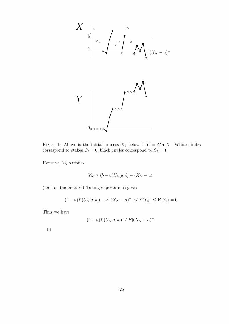
Figure 1: Above is the initial process X, below is Y = C • X. White circlescorrespond to stakes Ci = 0, black circles correspond to Ci = 1.

However, YN satisfies

YN ≥ (b− a)UN [a, b]− (XN − a)−

(look at the picture!) Taking expectations gives

(b− a)E(UN [a, b])− E[(XN − a)−] ≤ E(YN) ≤ E(Y0) = 0.

Thus we have

(b− a)E(UN [a, b]) ≤ E[(XN − a)−].

26

Define U∞[a, b] = limN→∞ UN [a, b].

We say that a process X is bounded in L1 if there exists a constant K such that

E|Xn| ≤ K for each n = 1, 2, ... or, equivalently, K := supn E(|Xn|) < ∞.

Lemma 3. Let X be a supermartingale bounded in L1 (i.e. supn E(|Xn|) < ∞).

Then for any a, b ∈ R, a < b, we have

P(U∞[a, b] = ∞) = 0.

Proof

By Lemma 2 we have

(b− a)EUN [a, b] ≤ E[(XN − a)−] ≤ |a|+ E(|XN |) ≤ |a|+K < ∞, ∀N ≥ 1.

Letting N → ∞ and using Monotone Convergence Theorem (MON) we have

EU∞[a, b] < ∞. But then it must be that

P(U∞[a, b] = ∞) = 0.

Theorem 5. (Doob’s Forward Convergence theorem)

Let X be a supermartingale bounded in L1 (i.e. K = supn E|Xn| < ∞). Then,

almost surely, the limit X∞ := limn→∞ Xn exists and is finite.

Proof

Note that

A = ω : Xn(ω) does not converge to a limit in [−∞; +∞]= ω : lim inf

nXn(ω) < lim sup

nXn(ω)

= ∪a,b∈Q:a<bω : lim infn

Xn(ω) < a < b < lim supn

Xn(ω)

= ∪a,b∈Q:a<bω : U∞[a, b](ω) = ∞.

27

Since A is a countable union of subsets ω : U∞[a, b](ω) = ∞ of zero-probability

(previous Lemma applies!), we see that P(A) = 0, whence

limn

Xn exists a.s. in [−∞; +∞].

Show now that −∞ and ∞ are in fact excluded, i.e. limn Xn can only take finite

values a.s. Indeed, by Fatou’s Lemma we have

E(|X∞|) = E(lim infn

|Xn|) ≤ lim infn

E(|Xn|) ≤ K < ∞,

so that P(|X∞| < ∞) = 1.

Corollary 2. If X is a non-negative supermartingale, then, almost surely, the

limit X∞ := limn→∞Xn exists and is finite.

Proof. Non-negative X is bounded in L1, since E|Xn| = EXn ≤ E0 for each n.

Now Theorem 5 applies.

28

6 Martingales bounded in L2

One of the easiest ways of proving that a martingale M is bounded in L1 (needed

in Doob’s Convergence Theorem!) is to prove that it is bounded in L2 in the sense

that supnE(X2n) < ∞. (This is based on the simple fact that |Xn| ≤ X2

n + 1,

showing that E(X2n) < ∞ implies E|Xn| < ∞.)

Let M = (Mn : n ≥ 0) be a L2-martingale. Then for any time moments

0 ≤ s ≤ t ≤ u ≤ v the increments Mt − Ms and Mv − Mu are uncorrelated

(orthogonal in L2):

E[(Mt −Ms)(Mv −Mu)] = E[E((Mt −Ms)(Mv −Mu) | Fu)]

= E[(Mt −Ms)E(Mv −Mu) | Fu)] = 0,

since E(Mv −Mu | Fu) = 0 in the martingale case. Now the simple formula

Mn = M0 +n∑

i=1

(Mi −Mi−1) (7)

expresses Mn as the sum of uncorrelated terms, and therefore we obtain

E(M2n) = E(M2

0 ) +n∑

i=1

E(Mi −Mi−1)2. (8)

Note that all terms on the right-hand side are non-negative, so that the second

moment (and also the variance) of Mn grow monotonically together with n.

Theorem 6. Let M be a L2-martingale. Then

(a) M is bounded in L2 if and only if

∞∑

k=1

E(Mk −Mk−1)2 < ∞. (9)

(b) If M is bounded in L2, then Mn → M∞ a.s. and in L2.

Proof. (a) For (8) the L2-boundedness of M is equivalent to (9). (b) Suppose now

(9) holds. Then M is bounded in L2, hence also in L1. By Doob’s Convergence

Theorem we have that Mn → M∞ =: lim infMn a.s.. Show now the convergence

29

in L2, meaning that limn E(M∞ −Mn)2 = 0. For orthogonality of increments we

have

E(Mn+r −Mn)2 =

n+r∑

k=n+1

E(Mk −Mk−1)2.

Letting r → ∞ and applying Fatou’s Lemma, we obtain

E(M∞ −Mn)2 = E(lim inf

r(Mn+r −Mn)

2) ≤ lim infr

E(Mn+r −Mn)2

=∞∑

k=n+1

E(Mk −Mk−1)2,

which tends to 0 when n → ∞ (the residual sum of a convergent series!). Hence

limn

E(M∞ −Mn)2 = 0,

so that Mn → M∞ in L2.

30

7 Doob Decomposition. Quadratic Variation

Theorem 7. (Doob decomposition)

(a) Let X be an adopted process, with Xn ∈ L1, ∀n. Then X can be represented

in the form

X = X0 +M + A,

where M is a martingale null at 0, and A is a previsible process null at 0. More-

over, this decomposition is unique up to the a.s. equivalence in the sense that

if X = X0 + M ′ + A′ is another such decomposition, then PM = M ′, A =

A′, ∀n = 1.

(b) The process X is a submartingale if and only if the process A is increasing

a.s.

Proof. (a) Define

A0 = 0,

An =n∑

i=1

E(Xi −Xi−1 | Fi−1), n ≥ 1,

and

Mn = Xn −X0 − An.

Show that A and M satisfy the conditions stated in the theorem. Obviously, A

is predictable (An ∈ Fn−1). Check that M is a martingale:

E(Mn −Mn−1 | Fn−1) = E(Xn −Xn−1 − (An − An−1) | Fn−1) (10)

= E(Xn −Xn−1 − (Xn −Xn−1) | Fn−1) (11)

= 0. (12)

Thus M is a martingale.

(b) If X is a submartingale, then E(Xi −Xi−1 | Fi−1) ≥ 0, ∀i, and we have

An =n∑

i=1

E(Xi −Xi−1 | Fi−1) ≥ An−1, (13)

so that A is increasing.

31

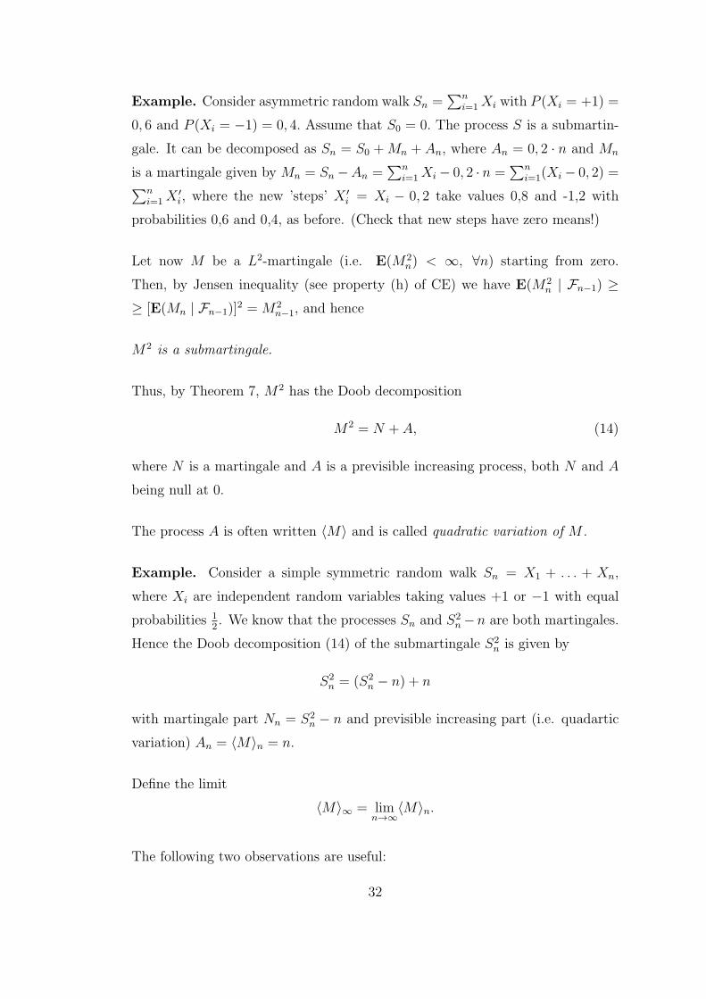
Example. Consider asymmetric random walk Sn =∑n

i=1 Xi with P (Xi = +1) =

0, 6 and P (Xi = −1) = 0, 4. Assume that S0 = 0. The process S is a submartin-

gale. It can be decomposed as Sn = S0 +Mn + An, where An = 0, 2 · n and Mn

is a martingale given by Mn = Sn −An =∑n

i=1 Xi − 0, 2 · n =∑n

i=1(Xi − 0, 2) =∑n

i=1 X′i, where the new ’steps’ X ′

i = Xi − 0, 2 take values 0,8 and -1,2 with

probabilities 0,6 and 0,4, as before. (Check that new steps have zero means!)

Let now M be a L2-martingale (i.e. E(M2n) < ∞, ∀n) starting from zero.

Then, by Jensen inequality (see property (h) of CE) we have E(M2n | Fn−1) ≥

≥ [E(Mn | Fn−1)]2 = M2

n−1, and hence

M2 is a submartingale.

Thus, by Theorem 7, M2 has the Doob decomposition

M2 = N + A, (14)

where N is a martingale and A is a previsible increasing process, both N and A

being null at 0.

The process A is often written 〈M〉 and is called quadratic variation of M .

Example. Consider a simple symmetric random walk Sn = X1 + . . . + Xn,

where Xi are independent random variables taking values +1 or −1 with equal

probabilities 12. We know that the processes Sn and S2

n−n are both martingales.

Hence the Doob decomposition (14) of the submartingale S2n is given by

S2n = (S2

n − n) + n

with martingale part Nn = S2n − n and previsible increasing part (i.e. quadartic

variation) An = 〈M〉n = n.

Define the limit

〈M〉∞ = limn→∞

〈M〉n.

The following two observations are useful:

32

(i) M is bounded in L2 if and only if E〈M〉∞ < ∞.

Indeed, since E(M2n) = E(An) is increasing in n, we have supE(M2

n) = E〈M〉∞.

(ii) 〈M〉n − 〈M〉n−1 = E(M2n −M2

n−1 | Fn−1) = E[(Mn −Mn−1)2 | Fn−1].

Indeed, since E(Mn−1Mn | Fn−1) = Mn−1E(Mn | Fn−1) = M2n−1, we can write

E(M2n −M2

n−1 | Fn−1) = E(M2n − 2Mn−1Mn + 2Mn−1Mn −M2

n−1 | Fn−1)

= E(M2n − 2Mn−1Mn +M2

n−1 | Fn−1)

= E[(Mn −Mn−1)2 | Fn−1].

- the conditional variance of the increment of M .

33

8 Brownian motion

8.1 Transition to continuous time.Brownian motion.

So far, we have studied martingales with discrete time, t = 0, 1, 2, . . .. The

simpliest example was Simple Random Walk (SRW). In finance, however, it is

also useful to consider processes with continous time, where the time parameter

t ∈ R+ = [0,∞). For example, stock prices can change at any time instant within

a business day. Among random processes with continous time one of the most

important is so-called Brownian motion. Brownian motion is a simple continuous

stochastic process that is widely used in physics and finance for modeling random

behavior that evolves over time. Examples of such behavior are the random

movements of a molecule of gas or fluctuations in an asset’s price.

Brownian motion gets its name from the botanist Robert Brown (1828) who

observed in 1827 that tiny particles of pollen suspended in water moved erratically

on a microscopic scale; but he was not able to determine the mechanisms that

caused this motion. The physicist Albert Einstein published a paper in 1905

explaining that the motion was caused by water molecules randomly bombarding

the particle of pollen, and thus helping to firmly establish the atomic theory of

matter. Later on, starting in 1918, American mathematician Norbert Wiener

created a precise mathematical model for this phenomena. This is what we will

study now.

In order to define the Brownian motion, we start from Simple Random Walk

(SRW) and let its step sizes (both time step and space step) to go to 0. Denote

Xt = ∆x · (X1 +X2 + . . .+X[ t∆t

]),

where

Xi =

+1, with probability 1

2,

−1, with probability 12,

34

∆x - space step size,

∆t - time step size,

t∆t

- the number of time steps in the time interval [0, t].

SinceX1, X2, . . . , X[ t∆t

] are independent identically distributed (IID) random vari-

ables with mean value EXi = 0 and variance DXi = 1, then for each ∆x and

∆t we have EXt = 0 and DXt = (∆x)2[ t∆t]. When ∆t → 0,∆x → 0, then the

number of summands [ t∆t] increases unboundedly and according to the Central

Limit TheoremXt

∆x√

[ t∆t]

D→ N (0, 1).

By choosing the relationship between ∆x and ∆t such that (∆x)2

∆t= const =: C2

we get, on the limit, that Xt ∼ N (0, C√t). The limiting process Xt preserves

some important features of SRW:

(i) The increments of Xt are independent i.e. for 0 ≤ s ≤ t ≤ u ≤ v the

increments Xt −Xs and Xv −Xu are indpendent r.v. (the same is valid for

any n time intervals).

(ii) The increments of Xt are stationary i.e. the distribution of Xs+t −Xs only

depends on t (and not on s).

These properties suggest the following definition.

Definition 6 (Brownian motion). The random process Wt, t ≥ 0 is called

Brownian motion (Wieneri process), if

(i) W (0) = 0,

(ii) for all t > 0 the r.v. Wt ∼ N (0, C√t), where C > 0 is a constant,

35

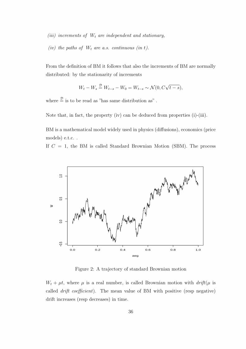
(iii) increments of Wt are independent and stationary,

(iv) the paths of Wt are a.s. continuous (in t).

From the definition of BM it follows that also the increments of BM are normally

distributed: by the stationarity of increments

Wt −WsD= Wt−s −W0 = Wt−s ∼ N (0, C

√t− s),

whereD= is to be read as ”has same distribution as” .

Note that, in fact, the property (iv) can be deduced from properties (i)-(iii).

BM is a mathematical model widely used in physics (diffusions), economics (price

models) e.t.c. .

If C = 1, the BM is called Standard Brownian Motion (SBM). The process

0.0 0.2 0.4 0.6 0.8 1.0

−0.5

0.00.5

1.0

aeg

W

Figure 2: A trajectory of standard Brownian motion

Wt + µt, where µ is a real number, is called Brownian motion with drift(µ is

called drift coefficient). The mean value of BM with positive (resp negative)

drift increases (resp decreases) in time.

36

8.2 Some properties of Brownian motion

1) Finite-dimensional distributions of SBM

The joint distribution of (Wt1 ,Wt2 , . . . ,Wtn) where 0 < t1 < t2 < . . . < tn can

easily be calculated.

For each ti the density of Wti is

fWti(x) =

1√2πti

e− x2

2ti ,

provided that C = 1. Since the equalities

Wt1 = x1

Wt2 = x2

. . .Wtn = xn

are equivalent to the equalities

Wt1 = x1

Wt2 −Wt1 = x2 − x1

. . .Wtn −Wtn−1 = xn − xn−1

and since the increments Wt1 ,Wt2 − Wt1 , . . . ,Wtn − Wtn−1 are independent, we

have

fWt1 ,...,Wtn(x1, . . . , xn) =

= fWt1 ,Wt2−Wt1 ,...,Wtn−Wtn−1(x1, x2 − x1, . . . , xn − xn−1) =

= fWt1(x1) · fWt2−Wt1

(x2 − x1) · . . . · fWtn−Wtn−1(xn − xn−1) =

=1√2πt1

e−x1

2

2t1 · 1√2π(t2 − t1)

e− (x2−x1)

2

2(t2−t1) · . . . · 1√2πtn − tn−1

e− (xn−xn−1)

2

2(tn−tn−1) .

The formula obtained can be used for many purposes.

37

2) Conditional distribution.

Let’s use the formula above to solve one particular problem. Suppose we know

that at time t BM has taken value Wt = B. Let s be an earlier time, s < t.

What is the conditional distribution of Ws given the event Wt = B? It is known

that the conditional density is the ratio of joint density and the density of the

condition, we can calculate

fWs|Wt(x|B) =

fWs,Wt(x,B)

fWt(B)

=

=

1√2πs

· ex2

2s · 1√2π(t−s)

· e(B−x)2

2(t−s)

1√2πt

· eB2

2t

= . . . =1√

2π st(t− s)

· e−t(x−B s

t )2

2s(t−s) .

Hence, the conditional distribution of Ws is normal distribution with mean B · st

and variance s(t−s)t

.

3) First passage time.

Let W0 = 0 and a > 0. We are interested in the time which elapses before BM

attains the level a. We call it the first passage time to the point a and denote

Ta = infT : Wt = a. Ta is a random variable since its value depends on the

path of BM (on ω.) Let’s find its distribution function FTa(t) = PTa ≤ t.

Using the formula of total probability, we have:

PWt ≥ a = PWt ≥ a|Ta ≤ t · PTa ≤ t+ PWt ≥ a|Ta > t · PTa > t.

For symmetry of normal distribution PWt ≥ a|Ta ≤ t = 12. At the same time

obviously PWt ≥ a|Ta > t = 0. Therefore PWt ≥ a = 12PTa ≤ t, and

PTa ≤ t = 2PWt ≥ a.

Since Wt ∼ N(0,√t), we have

FTa(t) = PTa ≤ t = 2

1√2πt

∫ ∞

a

e−x2

2t dx = 2[1− Φ

(a√t

)].

If a < 0, then by symmetry PTa ≤ a = 2[1− Φ(

|a|√t

)].

If a = 0, then T0 = 0. Taking all together, we have that, for any a,

PTa ≤ t = 2[1− Φ

( |a|√t

)]. (15)

38

By differentiating the distribution function above, one gets the density function

of Ta. For a > 0 it calculates as

fTA(t) = F ′

Ta(t) = −2ϕ(

a√t) · (−a

2) · t− 3

2 =a√2πt3

e−a2/2t.

This distribution is called inverse Gaussian distribution (also Wald distribution).

From (15) it is also seen that if t → ∞, then

P(Ta < ∞) = limt→∞

P(Ta ≤ t) = 1. (16)

4) Maxima of Brownian motion .

If a > 0, then Pmax0≤s≤t Ws ≥ a = PTa ≤ t = 2[1− Φ(

|a|√t

)].

If a < 0, then Pmax0≤s≤t Ws ≥ a = 1.

5) Brownian motion between two boundaries

Let A > 0, B > 0. Let us find the probability that, starting from 0, BM reaches

level A before −B. Recall that in the case of SRW the answer to the same

question is BA+B

. As the same answer remains true for any time and space steps

sizes, we have

PWt reaches A before − B = PTA < TB =B

A+ B.

39

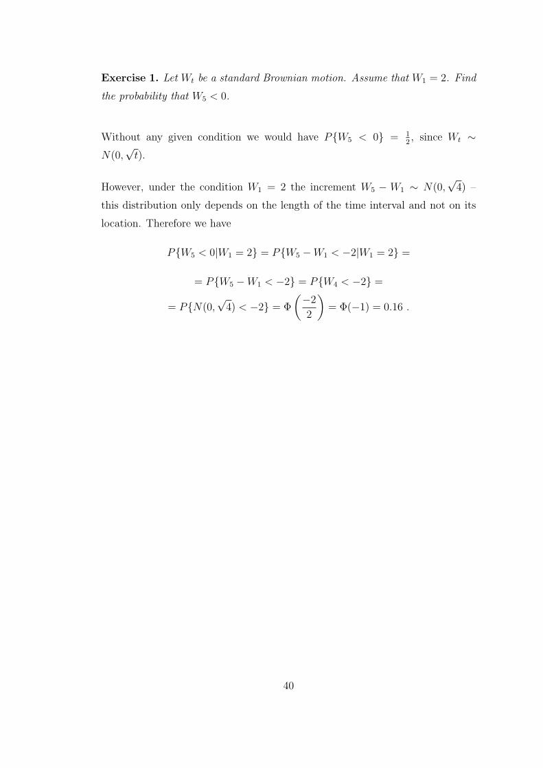
Exercise 1. Let Wt be a standard Brownian motion. Assume that W1 = 2. Find

the probability that W5 < 0.

Without any given condition we would have PW5 < 0 = 12, since Wt ∼

N(0,√t).

However, under the condition W1 = 2 the increment W5 − W1 ∼ N(0,√4) –

this distribution only depends on the length of the time interval and not on its

location. Therefore we have

PW5 < 0|W1 = 2 = PW5 −W1 < −2|W1 = 2 =

= PW5 −W1 < −2 = PW4 < −2 =

= PN(0,√4) < −2 = Φ

(−2

2

)= Φ(−1) = 0.16 .

40

9 Martingales with continous time

Many important concepts and results that are known for martingales with discrete

time can be transferred to continuous time without any major change.

Let (Ω,F ,P) be a probability space and let t be a real-valued parameter inter-

preted as time. Most often, t takes values from the half-line R+ or finite interval

[0, T ].

Definition 7. A family of σ-algebras Ft, t ≥ 0 is called a filtration, if

1) all its members Ft are sub-σ-algebras of F and, 2) for s < t one has Fs ⊆ Ft.

As in the case of dicsrete time, we are mainly interested in the natural filtration

FXt , t ≥ 0, generated by a random process X. As before, FX

t contains the

information induced by the random process X within the time interval [0, t]. It

means that an event A ∈ FXt if and only if one can decide whether A ocurred or

not on the basis of the trajectory Xs, 0 ≤ s ≤ t that the process X generates

by time t.

Definition 8. If Yt, t ≥ 0 is a random process such that for each t the random

variable Yt is Ft-measurable, then it is said that the process Y is adopted to

filtration Ft, t ≥ 0.

Examples:

1. The random process Zt =∫ t

0Xsds is adopted to the filtration FX

t , t ≥0, since knowing the path of X within time interval [0, t] is sufficient to

determine Zt.

2. The process Mt = max0≤s≤t Ws is adopted to the filtration FWt , t ≥ 0.

3. The process Zt = W 2t+1 −W 2

t is not adopted to the filtration FWt , t ≥ 0.

Similarly to discrete time we define martingales with continous time.

41

Definition 9. Let (Ω,F ,P) be a probability space endowed with a filtration

Ft, t ≥ 0. A random process Mt, t ≥ 0 is called a martingale, if

1. M is adopted to the filtration Ft, t ≥ 0,

2. E|Mt| < ∞, ∀t

3. for any s ≤ t we have E(Mt|Fs) = Ms a.s.

If the equality in 3. is replaced by the inequality ≤ (or ≥), then we speak about

a supermartingale (respectively submartingale).

Remark: Similarly, a martingale can be defined on a finite time interval [0, T ].

In the following mostly the filtration FWt , t ≥ 0, generated by a standard

Brownian motion W , is used.

Very important continous time martingales are related to Brownian motion.

Lemma 4. Let Wt be a standard Brownian motion and let Ft, t ≥ 0 be the

filtration induced by W. Then

1. Wt is a martingale,

2. W 2t − t is a martingale,

3. exp(σWt − σ2

2t) is a martingale (called exponential martingale).

Proof: The proofs resemble each other. Consider, for example, the process

Mt = W 2t − t. Obviously, E|Mt| < ∞. Find now

E(W 2t −W 2

s |Fs) = E[(Wt −Ws)2 + 2Ws(Wt −Ws)|Fs)]

= E[(Wt −Ws)2|Fs] + 2WsE[(Wt −Ws)|Fs]

= t− s.

So that

E(W 2t − t|Fs) = E(W 2

t −W 2s +W 2

s − (t− s)− s|Fs)

= (t− s) +W 2s − (t− s)− s = W 2

s − s,

42

and thus the process W 2t − t is a martingale.

Definition 10. A random variable T is called a stopping time with respect to the

filtration Ft, t ≥ 0, if for each t ≥ 0 the event T ≤ t ∈ Ft.

Let’s introduce a more general concept of local martingale.

Definition 11. A process Xt, t ≥ 0 is local martingale, if there exists a se-

quence of stopping times Tn, n = 1, 2, . . . such that the stopped process Xt∧Tn, t ≥

0 is a martingale for each n and

P[ limt→∞

Tn = ∞] = 1.

Every martingale is a local martingale (how to choose Tn?), however, a local

martingale need not be a martingale. This is the reason why we will assume

some boundedness condition to be satisfied in the following.

It is very useful to have a ’continuous’ version of Doob’s convergence theorem.

However, for that the trajectories of the martingale must be ’nice’ enough. In all

our examples below the trajectories are right continuous and have left limits or,

in short, cadlag (in French: continues a droite, limites a gauche ).

For example, continuous functions (like trajectories of Brownian motion) are au-

tomatically cadlag.

Theorem 8. (Stopping theorem in continous time)

If Mt, t ≥ 0 is a cadlag martingale w.r.t. the filtration Ft, t ≥ 0 and τ1, τ2

are bounded stopping times, τ1 ≤ τ2 ≤ K, then

E|Mτ2 | < ∞

and

E(Mτ2|Fτ1) = Mτ1 , P− a.s. (17)

Note: Let τ is a bounded stopping time. Then, by choosing τ1 = 0, τ2 = τ, and

by taking expectations from both sides in (17), we have EMτ = EM0.

43

We next consider an interesting application of the stopping theorem.

Lemma 5. Let Wt be a standard Brownian motion and let Ta be the first passage

time of level a, Ta = inft ≥ 0 : Wt = a. Then for any θ > 0

E[e−θ Ta

]= e−

√2θ|a| (18)

Proof. Assume that a ≥ 0 (the case a < 0 can be handled by symmetry).

Consider the martingale Mt = exp(σWt − σ2t/2). As the stopping time Ta is

not bounded, Theorem 8 does not apply directly. Instead, let’s consider bounded

stopping times τ1 = 0 and τ2 = Ta ∧ n. Then, by Theorem 8, we have

E(MTa∧n) = EM0 = 1, ∀n.

Show now that EMTa= limn E(MTa∧n). First recall that Ta < ∞ a.s. (cf the

formula (16)), hence starting from some value of n we have Ta < n and therefore

MTa∧n → MTaa.s.

At the same time the stopped martingale MTa∧n is bounded from both sides:

indeed, for WTa∧n ≤ a we have

0 ≤ MTa∧n = exp

(σWTa∧n −

σ2

2(Ta ∧ n)

)< eσa.

Therefore the bounded convergence theorem applies, giving us

EMTa= lim

nE(MTa∧n) = 1.

From the other side, by the definition ofMt, the expectation EMTacan be written

as

EMTa= E

[e(σa−

12σ2Ta)

].

Hence we have

1 = E[e(σa−

12σ2Ta)

],

and by choosing σ2 = 2θ, we obtain the required formula (18).

The Lemma above can be used, for example, for the calculation of ETa. (Expected

value of Ta can be expressed via its moment generating function m(θ) = E(eθTa),

namely, ETa = m′(0).) Try to show that ETa = ∞!

44

10 Stochastic integral

Our aim here is to give a meaning to the integral∫ t

0Xs dMs, where X is an

adopted process and M is a martingale, e.g. Brownian motion. This new integral

is rather different from the classical Stiltjes integral. In fact, we have already done

a useful piece of work in this direction when considering discrete time martingales.

For discrete time martingales we have defined the martingale transform as the

process

Yn =n∑

i=1

Ci(Xi −Xi−1) =: (C •X)n,

which was interpreted as the total winnings of a player after the game n (recall

that Ci is the stake of the player on game i and Xi − Xi−1 is the net winnings

per unit stake in game i.) Most importantly, we have shown (Theorem 2) that

if the process Ci is predictable and X is a martingale, then the process Y is a

martingale again. At the same time, the formula of the martingale transform

above looks like a certain integral sum. Our next task is to define similar concept

(stochastic integral) for continuous time martingales. Stochastic integral is an

efficient tool to solve problems in various areas, including option pricing.

We first show that it is not possible to integrate with respect to continuous time

martingales in a traditional manner i.e. path-wise (as Riemann- Stiltjes integral).

10.1 Variation. Quadratic variation of Brownian motion

Let us consider a function f of a real variable. Variability of the function f

within the interval [a, b] can be described by dividing the interval into smaller

subintervals using cutting points a = t0 < t1 < . . . < tn = b and by summing up

the absolute values of the increments |f(ti)− f(ti−1|. Instead of absolute values,

one could also use the squares, cubes etc. In order to avoid the dependence of

the result on the interval partition method, we allow the number of cut-points n

to approach infinity. We thus reach the following definition.

45

Definition 12. The p-variation of a function f over the interval [a, b] is defined

as

V arp(f ; a, b) = lim sup‖πn‖→0

n∑

i=1

|f(ti)− f(ti−1)|p,

where πn is a partition of [a, b] by cutting points a = t0 < t1 < . . . < tn = b, and

‖πn‖ is the length of the longest subinterval of πn.

It is easy to see that when f is continuous and the partition is fine enough, so

that the increments |f(ti)− f(ti−1| are small numbers (smaller than 1), then the

higher is the order p the less is the result. Thus for p > q the p-variation is less

than the q-variation.

At the same time, while studying martingales, we have used the term ’quadratic

variation’: the quadratic variation of a martingale M was a predictable process A

such that the difference M2−A is again martingale. For example, for a standard

Brownian motion W the process W 2t − t is a martingale, and hence t is the

quadratic variation of standard Brownian motion. The question arises whether

such a coincidence of terminology is justified. The positive answer is provided by

the following lemma. Consider a partition of the interval [0, t]

πn : 0 = t0 < t1 < . . . < tn = t

and let us denote

∆i = ti − ti−1, i = 1, 2, . . . , n

∆Wi = Wti −Wti−1,

Qn(t) =n∑

i=1

(Wti −Wti−1)2 =

n∑

i=1

(∆Wi)2.

Lemma 6. The following (mean-square) convergence takes place:

E[Qn(t)− t]2 → 0, n → ∞.

Proof. The increments of Brownian motion ∆Wi are independent and ∆Wi ∼N(0,

√∆i). Therefore

EQn(t) =n∑

i=1

E(∆Wi)2 =

n∑

i=1

∆i = t.

46

At the same time the variance

D(Qn(t)) =n∑

i=1

D((∆Wi)2) =

n∑

i=1

[E(∆Wi)4 −∆2

i ].

It is well known that the 4-th order moment of a N(0, 1)– distributed random

variable is 3, thus E(W 41 ) = 3. Hence, by taking into account the stationarity of

increments, we have

E(∆Wi)4 = E(Wti −Wti−1

)4 = EW 4ti−ti−1

= EW 4∆i

= E(√

∆iW1

)4= 3∆2

i ,

from which

D(Qn(t)) = 2n∑

i=1

∆2i .

Therefore, if ‖πn‖ = max∆i → 0, then

D(Qn(t)) ≤ 2‖πn‖ ·n∑

i=1

∆i = 2t ‖πn‖ → 0.

Since

D(Qn(t)) = E(Qn(t)− t)2,

the proof is completed.

Now it is not difficult to show that the variation (1-variation) of Brownian motion

is unbounded.

Corollary. The trajectories of Brownian motion have a.s. unbounded variation,

i.e. V ar1(W ; 0, t) = ∞.

Proof. Obviously, the following inequalities are valid:

Qn(t) =n∑

i=1

(∆Wi)2

≤ maxi

|∆Wi| ·n∑

i=1

|∆Wi|

≤ maxi

|∆Wi| · V ar1(W ; 0, t). (19)

We now let ‖πn‖ = max∆i → 0. Since the trajectories of Brownian motion are

uniformly continuous in the interval [0, t], we have the convergence maxi |∆Wi| →

47

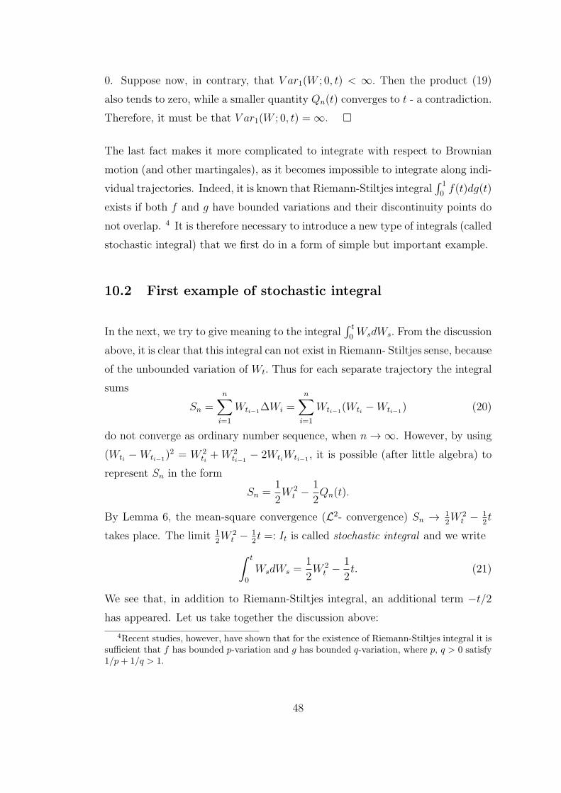
0. Suppose now, in contrary, that V ar1(W ; 0, t) < ∞. Then the product (19)

also tends to zero, while a smaller quantity Qn(t) converges to t - a contradiction.

Therefore, it must be that V ar1(W ; 0, t) = ∞.

The last fact makes it more complicated to integrate with respect to Brownian

motion (and other martingales), as it becomes impossible to integrate along indi-

vidual trajectories. Indeed, it is known that Riemann-Stiltjes integral∫ 1

0f(t)dg(t)

exists if both f and g have bounded variations and their discontinuity points do

not overlap. 4 It is therefore necessary to introduce a new type of integrals (called

stochastic integral) that we first do in a form of simple but important example.

10.2 First example of stochastic integral

In the next, we try to give meaning to the integral∫ t

0WsdWs. From the discussion

above, it is clear that this integral can not exist in Riemann- Stiltjes sense, because

of the unbounded variation of Wt. Thus for each separate trajectory the integral

sums

Sn =n∑

i=1

Wti−1∆Wi =

n∑

i=1

Wti−1(Wti −Wti−1

) (20)

do not converge as ordinary number sequence, when n → ∞. However, by using

(Wti −Wti−1)2 = W 2

ti+W 2

ti−1− 2WtiWti−1

, it is possible (after little algebra) to

represent Sn in the form

Sn =1

2W 2

t − 1

2Qn(t).

By Lemma 6, the mean-square convergence (L2- convergence) Sn → 12W 2

t − 12t

takes place. The limit 12W 2

t − 12t =: It is called stochastic integral and we write

∫ t

0

WsdWs =1

2W 2

t − 1

2t. (21)

We see that, in addition to Riemann-Stiltjes integral, an additional term −t/2

has appeared. Let us take together the discussion above:

4Recent studies, however, have shown that for the existence of Riemann-Stiltjes integral it issufficient that f has bounded p-variation and g has bounded q-variation, where p, q > 0 satisfy1/p+ 1/q > 1.

48

• For each separate trajectory Wt(ω) the integral sum Sn(ω) does not con-

verge.

• At the same time, the average of Sn (over all ω) is equal to It =12W 2

t − 12t,

so that E(Sn − It) = 0 for each n.

• Sn fluctuates around the process It and its deviation from It vanishes when

n increases to infinity: for each t we have E(Sn − It)2 → 0 (convergence in

L2).

Thus the stochastic integral It is a random process which is not necessarily close

to the integral sum Sn for each separate trajectory, but it works well (as much as

possible) for all trajectories simultaneously.

It is important to note, that the integral sum Sn =∑n

i=1 Wti−1(Wti −Wti−1

) is a

martingale transform and therefore (by Theorem 2) it is a martingale. We also

know that the limit process It =12W 2

t − t2is a martingale (see Lemma 4, assertion

2)).

Comment: If we define Sn slightly differently from (20), Sn =∑n

i=1 Wti∆Wi,

using ti = (ti−1 + ti)/2 (instead of ti−1), the process Sn stops to be a martingale.

The integral obtained by such an alternative construction is called Stratonovich

integral and it has useful technical applications.

We now proceed to a more general definition of the stochastic integral. In doing

that we do not restrict ourselves with integration merely w.r.t. the Brownian

motion.

10.3 Definition of stochastic integral

In order to define a stochastic integral in general case, we follow the standard

scheme:

1) the stochastic integral is first defined for ”simple” processes (resembles a mar-

tingale transform),

49

2) a general process is represented as the limit of simple processes,

3) the stochastic integral of a general process is defined as the limit of integrals

of respective simple processes.

10.3.1 Stochastic integral of simple process

Let T = [0,∞) and let Ft, t ∈ T be a filtration. Let M be a continuous square

integrable martingale w.r.t. the filtration Ft, t ∈ T.

Definition 13. The process η is called a simple process if there exists a finite

number of time instances 0 = t0 < t1 < · · · < tn = ∞ and random variables

ξi, i = 1, 2, . . . , n, with finite variances such that ξi is Fti−1-measurable for each

i and

ηt =n∑

i=1

I[ti−1,ti)(t)ξi.

Definition 14. The stochastic integral of a simple process η with respect to a

martingale M is defined as the process

Intt =

∫ t

0

ηs dMs : =nt∑

i=1

ξi(Mti −Mti−1) + ξnt+1(Mt −Mtnt

)

≡n∑

i=1

ξi(Mt∧ti −Mt∧ti−1),

where nt is an integer such that tnt≤ t < tnt+1.

Notice that the last formula has the structure of a martingale transform (3).

Therefore, by Theorem 2, the process Intti is a martingale as well.

It is easy to see that by choosing η ≡ 1, we obtain an useful formula

∫ t

0

dMs = Mt −M0,

as in the case of classical R-S integral.

50

10.3.2 Stochastic integral of continuous process

Let M be a martingale and let Z be an adopted and continuous process such that

E(

∫ t

0

Z2s d〈M〉s) < ∞ ∀t > 0.

Definition 15. The stochastic integral of a process Z with respect to a martingale

M is defined as the limit (in L2)

Intt =

∫ t

0

Zs dMs = lim‖πn‖→0

n∑

i=1

Zti−1(Mti −Mti−1

),

where πn is a partition of [0, t] into n subintervals:

0 = t0 < t1 < · · · < tn = t.

Theorem 9. Stochastic integral has following properties:

(i) The process (Intt)t∈[0,∞) is a square integrable martingale.

(ii) The quadratic variation of Int is the process

〈Int〉t =∫ t

0

Z2s d〈M〉s.

Proof: The properties are relatively easy to prove for simple processes. The

second property is known as isometry.

Generally speaking, the definition above is not suitable for immediate calcu-

lations, except for simple processes. (The same is true for classical Riemann

integral!). Therefore certain rules have been worked out to calculate stochastic

integrals in practice. Here the central role is played by so called Ito formula.

51

11 Ito formula and its applications

Consider an stochastic process Xt, which can be decomposed as

Xt = X0 + Vt +Mt, (22)

where

– Mt is a martingale with continuous trajectories that have non-zero quadratic

variation, V ar2 > 0 (such trajectories are called ’rough’, e.g. Brownian motion),

– Vt is an adopted process with continuously differentiable (or ’smooth’) trajecto-

ries that have finite variation, V ar1 < ∞, and zero quadratic variation, V ar2 = 0.

Such processes Xt are called semimartingales.

We are interested in an expression for the increment f(Xt) − f(X0) for some

functions f .

In classical analysis, it is known that if Xt is a ”common” process (e.g. with

continuously differentiable trajectories) then the Newton-Leibnizi formula gives

f(Xt)− f(X0) =

∫ t

0

f ′(Xs)dXs.

However, for more general processes (22) the answer is different, as shows the Ito

formula below.

11.1 Ito formula

Let f be twice continuously differentiable function. Then

f(Xt)− f(X0) =

∫ t

0

f ′(Xs)dVs +

∫ t

0

f ′(Xs)dMs +1

2

∫ t

0

f ′′(Xs)d〈M〉s . (23)

The second integral at the right hand side of Ito formula is a stochastic integral,

whereas the other two are traditional (Riemann-Stiltjes) integrals. Hence, the

stochastic integral can be expressed in terms of usual integrals. This is why the

52

Ito formula is so important.

Example 1. Let Wt be standard Brownian motion and Xt = Wt (i.e. the

decomposition (22) contains only the martingale part while X0 = Vt = 0. Using

Ito formula, show that∫ t

0WsdWs = 1

2W 2

t − 12t (that, in fact, we know already

from before) (21).)

Hint: Take f(x) = x2.

The proof of Ito formula. We present only the basic idea of the proof. For

simplicity, let Vt = 0 and let Mt = Wt - a standard Brownian motion. Since the

quadratic variation is 〈W 〉s = s, we need to show that

f(Xt)− f(X0) =

∫ t

0

f ′(Xs)dWs +1

2

∫ t

0

f ′′(Xs)ds. (24)

Let us consider a partition of the interval [0, t] by points 0 = t0 < t1 < . . . < tn =

t. Then

f(Xt)− f(X0) ≡n∑

i=1

[f(Xti)− f(Xti−1

)].

In each subinterval we apply usual Taylor’s formula:

f(Xt)− f(X0) =n∑

i=1

f ′(Xti−1)(Wti −Wti−1

) +1

2

n∑

i=1

f ′′(Xξi)(Wti −Wti−1)2,

where ξi ∈ [ti, ti−1]. When the partition gets finer, so that the maximum length of

subintervals tends to zero, the first sum converges (in mean square) to stochastic

integral∫ t

0f ′(Xs)dWs. At the same time, in the second term the square of the

increment of the Brownian motion (Wti − Wti−1)2 can be approximated by its

mean value ∆i = ti − ti−1 (related calculations were made in the proof of the

lemma 6 where it came out that the variance D((Wti − Wti−1)2) = 2∆2

i → 0).

Therefore, the second term can be approximated by the expression

12

∑ni=1 f

′′(Xξi)∆i, which converges to usual integral 12

∫ t

0f ′′(Xs)ds.

53

Example 2. A widely used model in financial mathematics to describe the

behaviour of a stock price St is the following:

dSt = St (µdt+ σdWt), (25)

where

µ shows relative change of the price per time unit (a constant in this model),

dWt is the random part of the price change, that within a short time interval ∆t

behaves like an increment of a Brownian motion ,

σ shows the importance of the random component in the development of the price

(volatility parameter).

The relationship above is, in fact, a short notation of the following equation:

St − S0 =

∫ t

0

Ssµds+

∫ t

0

SsσdWs. (26)

The equation (25) is called stochastic differential equation (SDE) . Our aim is to

solve this SDE for St. It turns out that the easiest way to do that is first to find

ln(St/S0).

Hint: apply Ito formula for f(x) = lnx.

54

11.2 Ito formula in differential form

df(Xt) = f ′(Xt)dXt +1

2f ′′(Xt)d〈M〉t . (27)

The formula (27) comes immediately from the Ito formula (23), being simply

its shorter (and more convenient) notation. Here the expression d〈M〉t is the

usual differential of the function 〈M〉t , however dXt is a symbol of (nn stochastic

differential), whose precise meaning is given by the notion of stochastic integral∫ t

0f ′(Xs)dXs.

Example 3. Solve the problem in Example 2, using the differential form of Ito

formula.

55

11.3 A generalization of Ito formula

Let the function f also depend on time, f = f(Xt, t), where the process Xt

is still of the form (22). Assuming that the function f(x, t) is smooth enough

(sufficiently times differentiable), the following formula is valid:

df(Xt, t) =∂f

∂t(Xt, t) dt+

∂f

∂x(Xt, t) dXt +

1

2

∂2f

∂x2(Xt, t) d〈M〉t . (28)

Example 4. Assume that a stock price St behaves in accordance with the

following model:

dSt = St (rdt+ σdWt),

where r is the risk free interest rate and σ is the price volatility. Show that then

the discounted price process e−rtSt is a martingale.

Hint: use f(x, t) = e−rtx.

56

Example 5. Find d (e−rtV (St, t)), where V (s, t) is known twice continuously

differentiable function and the price process St is driven by the equation dSt =

St (rdt+ σdWt).

Hint: Take f(s, t) = e−rtV (s, t).

57

The result is the following stochastic differential equation

d (e−rtV (St, t)) = e−rt

[−rV (St, t) +

∂V

∂t+ rSt

∂V

∂s+

1

2S2σ2∂

2V

∂s2

]dt+e−rtσSt

∂V

∂sdWt

Corrollary: If the function V = V (s, t) satisfies the relationship

∂V

∂t+ rs

∂V

∂s+

1

2s2σ2∂

2V

∂s2− rV = 0, ∀s, t (29)

then the coefficient of the term dt becomes zero and the result is the martingale

d (e−rtV (St, t)) = e−rtσSt∂V

∂sdWt.

We have discovered a relationship between random processes (SDE) and differ-

ential equations (PDE). The formula (29) is called Black-Scholes equation.

The fact that, under some circumstances, e−rtV (St, t) is a martingale can be used

to solve several problems in financial mathematics. This is based on exploiting

the martingale’s property to keep its mean value over the time. Let us consider

an example of this type.

Example 6. Option pricing

58

11.4 Ito formula for functions of several variables

Consider a function of several variables in the form f(x1, x2, . . . , xn, t), for exam-

ple∑n

i=1 xi+t.Our aim is to find the stochastic differential d f(X1t, X2t, . . . , Xnt, t).

We first introduce the concept of cross-variation.

Definition 16. The cross-variation of martingales M and N is the process

〈M,N〉t =1

4(〈M +N〉t − 〈M −N〉t) .

Some most important properties of cross-variation are:

1. 〈M,M〉t = 〈M〉t. (It suffices to take M = N in the definition)

2. If Int1t =∫ t

0ξs dMs ja Int2t =

∫ t

0ηs dNs, then

〈Int1, Int2〉t =∫ t

0

ξsηs d〈M,N〉s.

3. For independent Brownian motions 〈W1,W2〉t = 0.

Ito formula for functions of several variables

If f is twice continuously differentiable function, then

d f(X1t, X2t, . . . , Xnt, t) =∂f

∂t(−→X t, t) dt+

n∑

i=1

∂f

∂xi

(−→X t, t) dXit +

+1

2

n∑

i=1

n∑

j=1

∂2f

∂xi∂xj

(−→X t, t) d〈Mi,Mj〉t

where Xit is of the form Xit = Xi0 + Vit +Mit,

V is a term with ’nice’ properties (having finite variation), and M is a martingale.

Naide 7.

59

12 Change of measure. Girsanov’s theorem

12.1 Options

An option is a contract between a buyer and a seller that gives the buyer of

the option the right, but not the obligation, to buy or to sell a specified asset

(underlying) on or before the option’s expiration time, at an agreed price, the

strike price. In return for granting the option, the seller collects a payment (the

premium) from the buyer. Granting the option is also referred to as ”selling” or

”writing” the option. A call option gives the buyer of the option the right but

not the obligation to buy the underlying at the strike price. A put option gives

the buyer of the option the right but not the obligation to sell the underlying at

the strike price.

If the buyer chooses to exercise this right, the seller is obliged to sell or buy the

asset at the agreed price. If the option may only be exercised at expiration time

T then it is called European option. An American option, in contrary, may be

exercised on any trading day on or before expiration.

The price of the underlying St can rise by time T higher than strike price K. In

such case the owner of the option at time T executes his right to buy shares at

price K and sells them at the market price, earning ST − K per share. At the

same time, the seller of the option can lose the same amount of money, provided

he does not undertake anything during the option period. However, as we will

see below, the seller can take measures to avoid the loss.

Since the option never results in negative value, more exactly, at time T its value

is C(ST ) := max(ST − K, 0) , then it is natural that in return for granting the

option, the seller collects a payment (the premium) from the buyer. We see two

problems related to options:

• What is the fair price of the option (at the time of writing it but also at

any later time since we may want to sell the option on)?

60

• How can the seller (writer) of the option avoid possible loss caused by an

unfavorable change of the price of the underlying?

12.2 Option pricing

The basis for pricing an option is so called parity principle. According to that

principle, the fair price is the amount of money X0 such that if the seller, starting

trading with that amount at time 0 and using appropriate trading strategy, can

reach the same value XT at time T as the option itself , i.e. XT = C(ST ) =

max(ST −K, 0).

It is not difficult to show that when the option is priced differently from X0, there

will be a possibility for arbitrage where one side of the agreement (the buyer or

the seller) can earn a risk free profit.

In the following we assume that the stock price St is driven by the model

d St = St (µdt+ σ dWt), (30)

where µ is a constant component of the return, called drift, and σ is a constant

showing the importance of the random component of the return, called volatility.

Now consider an investor (= seller of the option) who invests the amount X0 at

time 0 partly in shares and puts the rest of the money onto a bank account with

risk free interest rate r. Then he starts trading the same stock putting the money

earned to the bank accunt and taking the money necessary for purchase of shares

from the same account (self-financing portfolio).

Let η(t) be the number of shares owned by the investor at time t. Then the value

Xt of the portfolio at time t consists of two parts: the value of shares η(t) · St

plus the money in the bank Xt − η(t)St. Let’s find the increment of the value of

such portfolio during a short time interval dt:

dXt = r [Xt − η(t)St] dt+ η(t) · dSt.

61

By using Ito formula and the market model (30) one can also calculate the change

of the discounted wealth:

d(e−rtXt) = η(t)d(e−rtSt)

(show this!). From here it is seen that as soon as the discounted price process

e−rtSt is a martingale, so does the discounted wealth e−rtXt. However, any mar-

tingale keeps its mean value over the time. Hence, its (non-random) initial value

X0 is equal to the mean value at any later time epoch, including time T :

X0 = e−r0X0 = E(e−rTXT ) = E(e−rTC(ST )) (31)

Only one question remains: whether the discounted price process e−rtSt is a martingale?

In order to decide that, we will find its stochastic differential, using Ito formula:

d (e−rtSt) = e−rtSt σ

(µ− r

σdt+ dWt

).

The result will definitely be a martingale if µ = r, since then the right hand side

reduces to the stochastic integral w.r.t. Wt, which is, as we know, a martingale.

However, it turns out that even when µ 6= r the whole expression in the brackets

in the last formula, Wt =µ−rσ

t+Wt, can be regarded as a martingale. For that, it

is only necessary to redefine appropriately the probabilities of the trajectories of

the initial Brownian motion Wt. In other words, the measure P must be changed

in such a way that Wt is martingale with respect to the new measure Q. How

this can be achieved? This possibility is granted by Girsanov’s Theorem (also

called Cameron-Martin Theorem) which also indicates the relationship between

the old and new meausres.

Theorem 10. (Girsanov’s Theorem)

Let Wt be a standard Brownian motion w.r.t. probability space (Ω, Ftt≥0, P).

Let Wt =∫ t

0θs ds+Wt, where the process θ is adopted to the filtration Ft and

satisfies the requirement E(e

12

∫ T

0 θ2sds)< ∞.

Then there exists a probability measure Q such that Wt is a standard Brownian

motion w.r.t. that measure. The measure Q is related to P via the formula

62

Q(A) =∫AMT (ω)P(dω), where

Mt = exp

(−∫ t

0

θs dWs −1

2

∫ t

0

θ2sds

).

The measure Q is called risk neutral or martingale measure. Let us apply Gir-

sanov’s Theorem in our case where we have θt ≡ µ−rσ. The assumption

E(e

12

∫ T

0 θ2sds)< ∞ is clearly fulfilled. Thus the existence of the martingale mea-

sure Q is guaranteed, and the option price is the expected value w.r.t. to that

new measure Q :

X0 = e−r0X0 = EQ(e−rTC(ST )). (32)

Finally, let’s explain the term ”risk neutral measure”. As

dWt = dWt −µ− r

σdt,

the market model (30) reduces (after simple calculations) to

d St = St (rdt+ σ dWt). (33)

The formula differs from the model (30) only in that µ is replaced by the risk

free interest rate r. We see that in the case of the measure Q the average return

of the stock price is equal to the risk free interest rate r. Hence the term interest

”risk neutral measure”.

Some remarks on how to calculate the option price as the expected value X0 =

EQ(e−rTC(ST )). Basically, there are two possibilities for that:

1. Simulation where a large number of price trajectories is generated, in

accordance with the market model (33). For each trajectory C(ST ) is found,

the results are averaged and multiplied by the discounting factor e−rT .

2. Analytical calculation of the expectation. This is only possible for some

simple pay-off functions C(St), like for example European type options. In

the latter case the result is well known as Black-Scholes pricing formula.

(a good exercise!)

63

C:/kalev/Documents and Settings/kalev/My Documents ... · in probability. The course starts with...

Documents

Transcript of C:/kalev/Documents and Settings/kalev/My Documents ... · in probability. The course starts with...