CJASR-12-13-119

Caspian Journal of Applied Sciences Research, 1(11), pp. 71-82, 2012

Available online at http://www.cjasr.com

ISSN: 2251-9114, ©2012 CJASR

71

A Novel Method for Determination of Grinding Wheel Loading

Hamed Adibi1, Seyed Mehdi Rezaei

2,٭ , Ahmed Aly Diaa Mohammed Sarhan

3

1, 2

Department of Mechanical Engineering, Amirkabir University of Technology, Tehran, Iran 1, 2

New Technology Research Center, Amirkabir University of Technology, Tehran, Iran

1,3Center of Advanced Manufacturing and Material Processing, Department of Engineering Design and

Manufacture, Faculty of Engineering, University of Malaya, Kuala Lumpur, 50603, Malaysia 3Department of Mechanical Engineering, Faculty of Engineering, Assiut University, Assiut, 71516, Egypt

*Corresponding Author: [email protected]

Wheel surface condition plays an important role in the grinding operation. Wheel loading which is chip

accumulation in the space between grains leads to the deterioration of wheel cutting ability and causes excessive

force and temperature. Identification of wheel loading is an important issue for optimizing the dressing intervals

but it can be a time consuming and an expensive process. A novel technique based on digital image processing to

determine the loading areas over the surface of CBN vitrified grinding wheels using the toolbox of MATLAB is

presented in this paper. The optical characteristics of the metal chips, the abrasive grains and wheel bond are

considered. Edge detection by means of Sobel method is applied to distinguish the wear flat area and chip metal

loading debris. Morphological operations including dilation and erosion procedure are applied to process the

image and calculate the ratios of the loading areas over the wheel surface. Experiments were performed to

examine the repeatability of the proposed technique. The results were verified by the use of a scanning electron

microscope.

Key words: Grinding, Wheel loading, Image processing.

1. INTRODUCTION

Due to the property of difficult-to-cut materials,

grinding is one of the effective machining methods

for superalloys (Zhong et al., 2001; Teichera et al.,

2008). In grinding of such ductile materials,

frequently removed chips may adhere into

porosities between abrasive grains or weld on top

of cutting grains which is called wheel loading

(Liu et al., 2007; Cai et al., 2003). This

phenomenon leads to dull wheel grains which

results in increased rubbing and excessive

vibration.

It raises the cutting force, temperature and

reduces wheel life (Cameron et al., 2010). CBN

vitrified grinding wheels provide an ideal solution

for many applications because of the possibility of

the wheel porosity and structure control in vitreous

bonds (Teichera et al. 2008; Wei et al., 2010).

However, this type of wheel is prone to loading

particularly in grinding of superalloys (Liu et al.

2007; Zhong and Hung, 2000). Dressing operation

must be applied optimally to prevent serious

detrimental damage to workpiece along with

improving of the wheel life. However for this kind

of wheel, frequent dressing should be avoided as it

is time consuming and expensive. Therefore, wheel

condition must be monitored periodically. Most

methods applied, monitor the grinding wheel

condition and utilize a touch-trigger probe

inspection. Sakamoto et al (1998) fitted a laser

micrometer directly on the wheel head of a CNC

surface grinder. Wheel loading was evaluated

qualitatively by comparing the profile of wheel

surface and micro-observation of the ground

surface. Mokbel and Maksoud (2000) applied

acoustic emission technique to monitor the

condition of grinding wheel. The inherent

sensitivity of acoustic-emission-based monitoring

is a serious problem of this method. Srivastava et

al applied X-Ray fluorescence technique for

loading measurement (Srivastava et al., 1985).

High energy was utilized by an X-Ray source to

determine wheel loading in grinding of lead and

mild-steel. Kim and Ahn used eddy current and

laser displacement sensors to measure loading on

the working wheel surface and the topography of

the dressed wheel to decide a proper dressing

interval (Kim and Ahn, 1999).

The most important limitation of these

techniques is the cost of equipments. Other wheel

monitoring techniques including chemical

detection, calorimetry, spectroscopy,

magnetization and radiotracing have been reported

but are all time consuming and expensive

processes (Mokbel and Maksoud, 2000 , Srivastava

et al. 1985, Kim and Ahn, 1999, Mao et al., 2010 ,

Lauer-Schmaltz and Konig,1980, Dornfeld et al.,

2003, Konig and Lauer-Schmaltz,1980). Today,

machine vision and digital image processing have

Adibi et al.


72

benefited the industries that employ it. As long as

computer processing speed continues to increase

while the cost of storage memory continues to

drop, the field of digital image processing will

grow. These widespread applications include

quality control in manufacturing (Mersmann,

2011), tool monitoring in machining processes

(Castejon et al., 2007) surface roughness control

(Al-Kindi and Shirinzadeh, 2007), wheel wear

monitoring in grinding operation (Lachance et al.,

2004; Yasui et al., 2001; Hosokawa and Yasui,

1996 ; Feng and Chen, 2007) and many others.

Image processing had been applied for examining

of grinding wheel surface condition by some

researchers (Lachance et al., 2004, Yasui et al.,

2001). (Yasui et al., (2001) developed a system for

extracting the cutting edge of a grinding wheel for

examination of the surface condition using Image

processing technique and had been applied for

calculating the cutting edge ratio. Feng applied this

technique for surface condition monitoring of

Al2O3 wheel (Feng and Chen, 2007). Lachance et

al used image processing for the measurement of

wear flat area of grinding wheels (Lachance et al.,

2004). This method was developed with a new

technique called region growing as a

supplementary solution for the detection of wear

flat areas. Although, scanning electron microscope

(SEM) is one of the best ways for observation of

wheel surface but it is very expensive and is not

practical for automated measurement.

In this paper, a new technique based on image

processing using Toolbox of MATLAB for chip

loading identification on CBN vitrified wheel is

presented. Due to fine chips and related loading

debris in grinding with CBN wheels, a portable

digital microscope with high resolution equipped

with adjustable LED light source is applied. Light

properties and optical characteristics of metal

loaded debris, abrasive grains and vitreous bond

were investigated to distinguish the chip loaded

debris from others. Edge detection, image

normalization, dilation and erosion process were

applied to process the image to calculate the ratios

of the loading areas over wheel surface. SEM

observations were used to assess the outcome of

this technique. Statistical analysis was used to

obtain the number of required images. Experiments

were also conducted to investigate the efficiency of

the technique in term of repeatability.

2. PROPERTIES OF LIGHT

The optical properties of crystals are obtained

using x-ray diffraction and direct chemical

analyses. These properties are the most reliable

tool available to distinguish and identify materials.

The optical properties depend on the manner that

visible light is transmitted through the crystal and

thus are dependent on crystal structure, crystal

symmetry, and chemical composition of the

materials (Nelson, 2012). Light is electromagnetic

radiation that has properties of waves. The

electromagnetic spectrum can be separated into

several bands founded on the wavelength of the

light waves. Visible light represents a slender

group of wavelengths between about 380 to 730

nm (Peatross and Ware, 2011). Human eyes

interpret these wavelengths as special colors. If

only a single wavelength come into the eyes, they

are interpreted as a certain color. As shown in

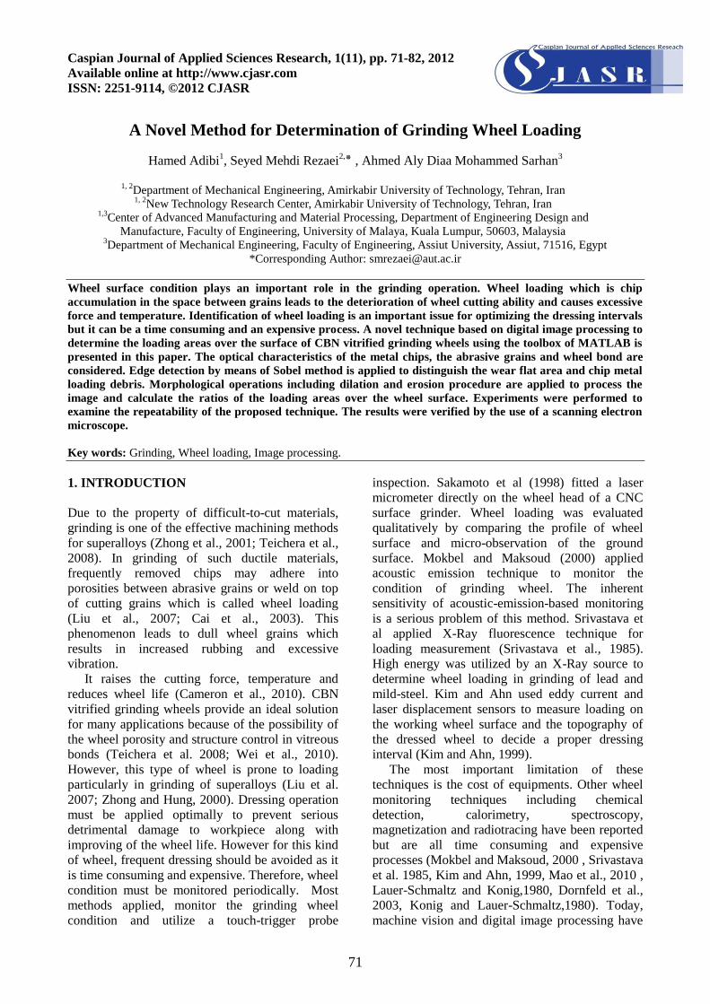
Fig.1, when light strikes an interface between two

substances with different refractive indices, it will

be reflected off the interface at the same entrance

angle. Alternatively it will be transmitted through

the substance with different refractive index which

depends on the transparency of the substance

(Peatross and Ware, 2011). The vitrified bond of

the wheel contains glass compositions of alumina-

silicate system. Abrasive grains are Cubic boron

nitride which is synthesized at pressures above 4.5

GPa and temperatures above 1500 K (Dou et al.,

2006). The light wavelength range which is

transparent to SiO2 is 0.2–4.5 μm. For Al2O3 this

is 0.15– 6.5 μm, therefore Al2O3 and SiO2 are

relatively transparent to the visible light (Feng and

Chen, 2007). Pure CBN is highly transparent or

slightly amber and can transmit over 99% of the

light with wavelengths in the range of 250-900 nm

(Song et al., 2010; Eremets et al., 1995). Different

colors can be produced depending on defects or an

excess of boron (less than 1%) (Haines et al.,

2001). Defects attributed to the effect of doping

solvent-catalysts (i.e. Li, Ca, or Mg nitrides) with

Al, B, Ti, or Si induces a change in the

morphology and color of CBN crystals (Bocquillon

et al., 1993). However, the CBN crystal is

transparent and the clogged metal chips on the

wheel cutting surface are opaque. Workpieces

ground were Inconel 738 in this investigation.

Therefore, when the light irradiates the CBN

vitrified wheel surface, metal chips adhered on it

reflect light robustly and appear brighter than other

area as shown in Fig.2. Image processing

technique applies this principle to calculate the

amount of chip loaded over the wheel surface.


73

3. PROPERTIES OF LIGHT

The procedure of proposed image processing

technique to analyze the captured image of the

wheel surface can be categorized in three stages.

Edge detection, Image segmentation and

Morphological operations are described separately

in the following sections.

3.1. Edge detection

Edge detection is the process of locating and

identifying sharp discontinuities in an image. The

discontinuities are sudden changes in pixel

intensity which characterize boundaries of the

object in an image. Edge detection has been used

by object recognition, target tracking,

segmentation, etc (Gonzalez et al., 2010). Several

edge detection methods are in use. Beside this

diversity, the majority of commonly used methods

are alike. Derivative operators are applied on

images and compute the gradient of several

directions and combine the result of each gradient.

The values of the gradient magnitude and

orientation are estimated using differentiation

masks. The magnitude of this derivative can be

used to detect the presence of the edges. These

several methods of edge detection include Sobel,

Prewitt, Roberts, and Canny. Sobel which is a

popular method was used in this work due to its

simplicity and common uses. In addition, the Sobel

operator holds a smoothing effect to reduce noise

which is one of the reasons for its popularity

(Gonzalez et al., 2010). Matlab contains various

toolboxes like image toolbox that has many

functions and algorithms. The function used in this

work was Standard Sobel operator and includes the

following steps.

Step 1: Convolution with gradient (Sobel) mask

Step 2: Magnitude of gradient.

Step 3: Thresholding.

First step is based upon a differentiation

operator that approximates the gradient of the

image intensity. As shown in Fig. 3, any point on

the Cartesian grid has its eight neighbor’s image

intensity or pixel value. Technically, this

differentiation operator using two convolutions

(one horizontal and one vertical) with a minimal

size kernel (3x3) to get local gradients from which

the gradient magnitude can be computed. The

directional derivative estimates vector G and was

defined as intensity difference divided by distance

to the neighbor. It is noted that the neighbors group

into antipodal pairs: (a , i ), (b , h), (c , g), (f , d).

The vector sum for this gradient estimate is

(Gonzalez et al., 2010):

0,1.1,0.

1,1.

1,1. dfhb

RR

ia

RR

gcG

(1)

Where 2R . This vector is obtained as

hbiagcdfiagcG 2/,2/ (2)

The resultant formula is given as follows (see, for

detail (Gonzalez et al., 2010) :

hbiagcdfiagcGG 2,.2.2 (3)

The weighting functions according to Fig. 4 for x

and y components were obtained by using the

above vector. In the second step the magnitude of

the derivative is calculated by the above masks.

The values can be used to detect the presence of

the edges of objects in the third step.

Fig. 1: Light striking between interface of different substance

3.2. Image segmentation

Image segmentation is a fundamental

processing step for many image processing

applications. There are many algorithms used for

image segmentation. Some of them segment an

image manually while others can segment

automatically (Meyer, 1992). Several general

purpose algorithms and techniques are available

for image segmentation. These techniques often

have to be combined with domain knowledge in

order to effectively solve an image segmentation

problem for a problem domain. The most common

method of image segmentation is the threshold

r

Refracte

d

Ray

i i Entranc

ed

Ray

Reflecte

d

Ray

Adibi et al.


74

technique. This method is based on a clip-level (or

a threshold value) to turn a gray-scale image into a

binary image. The key of this method is to decide

on the threshold value. Several popular methods

are used in industry including the maximum

entropy method, Otsu's method (maximum

variance), K-Means clustering and many others

(Gonzalez et al., 2010, Meyer, 1992). During the

thresholding process, individual pixels in an image

are labeled as "object" if their pixel value are

greater (or smaller) than threshold value. Other

pixels are labeled as "background".

Characteristically, an object pixel value is assigned

―1‖ while a background pixel value is assigned

―0.‖ Finally, a binary image is created by coloring

each pixel white or black, depending on a pixel's

label. Several different methods for choosing a

threshold exist. Users can manually choose a

threshold value, or a thresholding algorithm can

compute a value automatically. This is known as

automatic thresholding. A sophisticated and more

reliable approach might be to create a histogram of

the image pixel intensities and use the valley point

as the threshold. The histogram approach assumes

that there is some average value for the

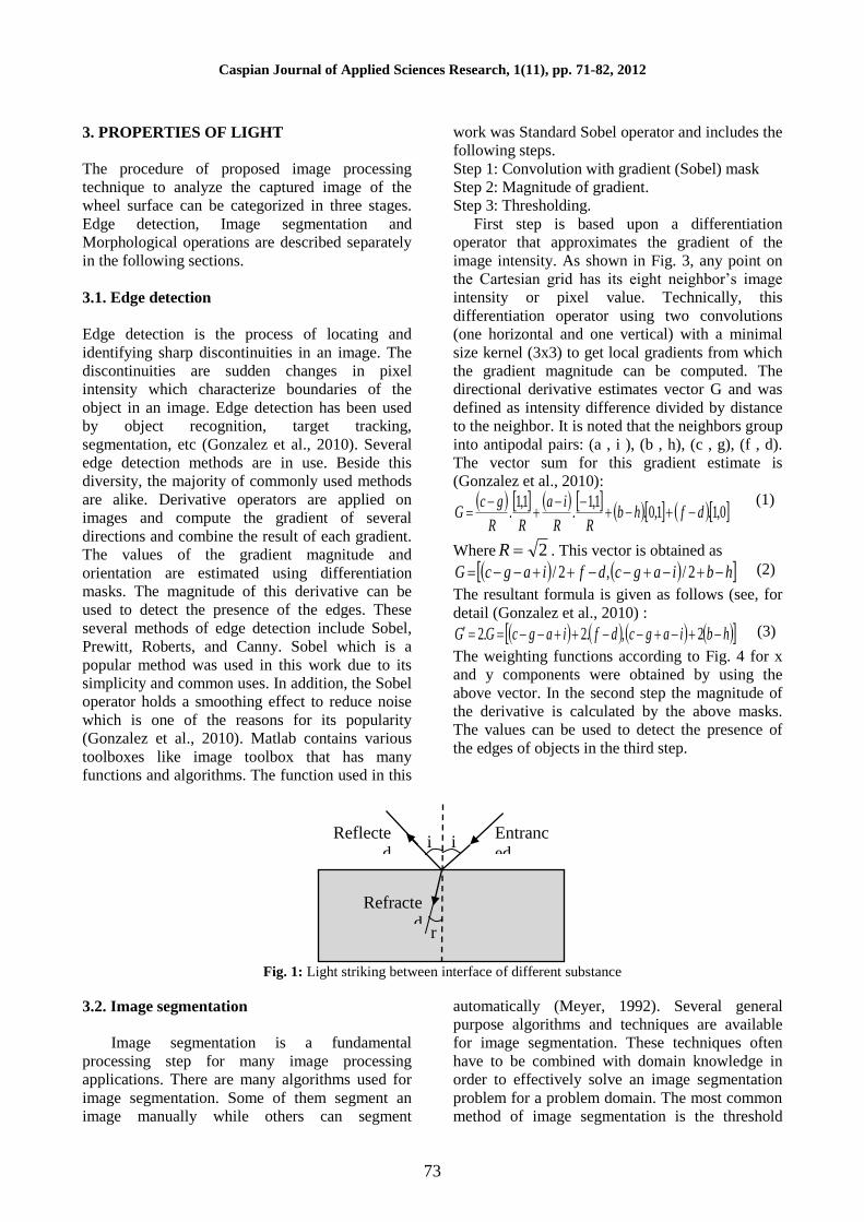
background and object pixels. A typical gray

scaled image of wheel surface is shown in Fig. 5.

The histogram of pixel value along the line A – B

is plotted in Fig. 5(b). The vertical axis of the

graph represents the pixel value. The magnitudes

of 0 and 255 correspond to black and white pixels,

respectively. It is evident that the pixel values of

metal loaded area are higher than 120

approximately. But the actual pixel values have

some variation around these average values.

However, this may be computationally expensive

and it is difficult to select an accurate threshold.

One method that is relatively simple and does not

require any specific knowledge of the image was

used in this work. It is also robust against image

noise. The iterative method was used in this work

is as follow:

(1) An initial threshold (T) is chosen; this can be

done randomly. (It was chosen 120 according to

histogram plot Fig. 5b in this study).

(2) The image is segmented into object and

background pixels as described above, creating

two sets:

G1 = {f(m,n) if f(m,n) >T} (object pixels)

G2 = {f(m,n) if f(m,n) ≤T} (background

pixels) (note, f(m,n) is the value of the pixel

located in the mth column, n

th row)

(3) The average of each set is computed.

M1 = average value of G1

M2 = average value of G2

(4) A new threshold is created that is the average

of M1 and M2

T′ = (M1 + M2)/2

Step 2 is used again with a new threshold

computed in step four. This is repeated until the

new threshold matches the one before convergence

was reached. This iterative algorithm is a special

one-dimensional case of the K-means clustering

algorithm, which has been proven to converge at a

local minimum (Meyer, 1992).

Fig. 2: CBN vitrified wheel surface image captured with digital microscope

20 µm

Metal

Loading

Debris

CBN grain

Vitrified

Bond


75

3.3. Binary morphological operations

Morphology is a widespread set of image

processing operations with process images based

on shapes. In a morphological operation, the value

of each pixel in the output image is based on a

comparison of the corresponding pixel in the input

image with its neighbors. The most basic

morphological operations are dilation and erosion

which were used in this work. In the

morphological dilation and erosion operations, the

state of any given pixel in the output image is

determined by applying a rule to the corresponding

pixel and its neighbors in the input image. Dilation

(sometimes called ―Minkowsky addition‖) is

defined as follows.

A ⊕ B = {c | c = a + b for some a ∈ A

and b ∈ B} (4)

Dilation works much like convolution: A kernel

is slide to each position in the image and at each

position ―apply‖ (union) the kernel. In the case of

morphology, this kernel B is called the structuring

element. This is useful for decomposing a single

large dilation into multiple smaller ones. Erosion

which is sometimes called ―Minkowsky

subtraction‖ is defined as follows.

AӨ B = {x | x + b ∈ A for every b ∈ B} (5)

Unlike dilation, erosion is not commutative.

After edge detection, the edges of segments

become some disconnected lines accompanied

with interior gap. They should be connected to

form the closed shapes by image dilation

processing step. A few noisy edges can also be

seen which are eliminated by image erosion

processing step.

By using the above image processing methods,

the features of loading areas can be extracted and

loading surfaces are identified. The following

demonstrates how edge detection is used. Image

segmentation and binary morphology to identify

loading of grinding wheel are described.

A b c

D e f

G h i

Fig. 3: Cartesian grid - eight neighbors for any point

+1 +2 +1

0 0 0

-1 -2 -1

+1 0 -1

+2 0 -2

+1 0 -1

(b) Y-direction (a) X-direction

Fig. 4: unit vector specifying the derivative’s direction

(b). histogram of intensity value along a line A-B. (a). Gray scaled Image

Fig. 5: Pixel Values of Image

A B

Adibi et al.


76

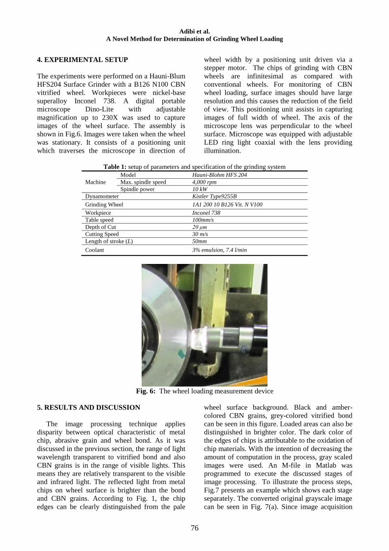
4. EXPERIMENTAL SETUP

The experiments were performed on a Hauni-Blum

HFS204 Surface Grinder with a B126 N100 CBN

vitrified wheel. Workpieces were nickel-base

superalloy Inconel 738. A digital portable

microscope Dino-Lite with adjustable

magnification up to 230X was used to capture

images of the wheel surface. The assembly is

shown in Fig.6. Images were taken when the wheel

was stationary. It consists of a positioning unit

which traverses the microscope in direction of

wheel width by a positioning unit driven via a

stepper motor. The chips of grinding with CBN

wheels are infinitesimal as compared with

conventional wheels. For monitoring of CBN

wheel loading, surface images should have large

resolution and this causes the reduction of the field

of view. This positioning unit assists in capturing

images of full width of wheel. The axis of the

microscope lens was perpendicular to the wheel

surface. Microscope was equipped with adjustable

LED ring light coaxial with the lens providing

illumination.

Table 1: setup of parameters and specification of the grinding system

Machine

Model Hauni-Blohm HFS 204

Max. spindle speed 4,000 rpm

Spindle power 10 kW

Dynamometer Kistler Type9255B

Grinding Wheel 1A1 200 10 B126 Vit. N V100

Workpiece Inconel 738

Table speed 100mm/s

Depth of Cut 20 μm

Cutting Speed 30 m/s

Length of stroke (L) 50mm

Coolant 3% emulsion, 7.4 l/min

Fig. 6: The wheel loading measurement device

5. RESULTS AND DISCUSSION

The image processing technique applies

disparity between optical characteristic of metal

chip, abrasive grain and wheel bond. As it was

discussed in the previous section, the range of light

wavelength transparent to vitrified bond and also

CBN grains is in the range of visible lights. This

means they are relatively transparent to the visible

and infrared light. The reflected light from metal

chips on wheel surface is brighter than the bond

and CBN grains. According to Fig. 1, the chip

edges can be clearly distinguished from the pale

wheel surface background. Black and amber-

colored CBN grains, grey-colored vitrified bond

can be seen in this figure. Loaded areas can also be

distinguished in brighter color. The dark color of

the edges of chips is attributable to the oxidation of

chip materials. With the intention of decreasing the

amount of computation in the process, gray scaled

images were used. An M-file in Matlab was

programmed to execute the discussed stages of

image processing. To illustrate the process steps,

Fig.7 presents an example which shows each stage

separately. The converted original grayscale image

can be seen in Fig. 7(a). Since image acquisition


77

may lead to noisy images, preprocessing

operations are usually performed before edge

detection. The most common preprocessing step in

image processing applications is image

normalization. Image normalization refers to

eliminating image variations (such as noise,

illumination, or occlusion) that are related to

conditions of image acquisition and are unrelated

to object identity.

(b) Normalized image (a) Original grey scaled image

(d) The consequence of dilation (c) edge detection

(f) The consequence of erosion (e) Holes in closed contour regions were filled

Fig.7: Steps of image processing of grinding wheel surface

Adibi et al.


78

The result of normalization of current example

is shown in Fig. 7(b). Edge segmented image by

Sobel operator can be seen in Fig. 7(c). Compared

to the original image, gaps can be seen in the lines

and areas surrounding the loading regions of the

gradient mask. As discussed before, these gaps will

disappear if the Sobel operated image is dilated.

The consequence of dilation is shown in Fig. 7(d).

The dilated gradient mask clearly shows the loaded

regions, but there are still holes in the interior of

the regions. To fill these holes any closed contour

pixels in images should be filled as shown in Fig.

7(e). Finally, in order to make the segmented

object look natural, the loaded areas were

smoothened by eroding the image which the

resulted image is shown in Fig. 7(f).

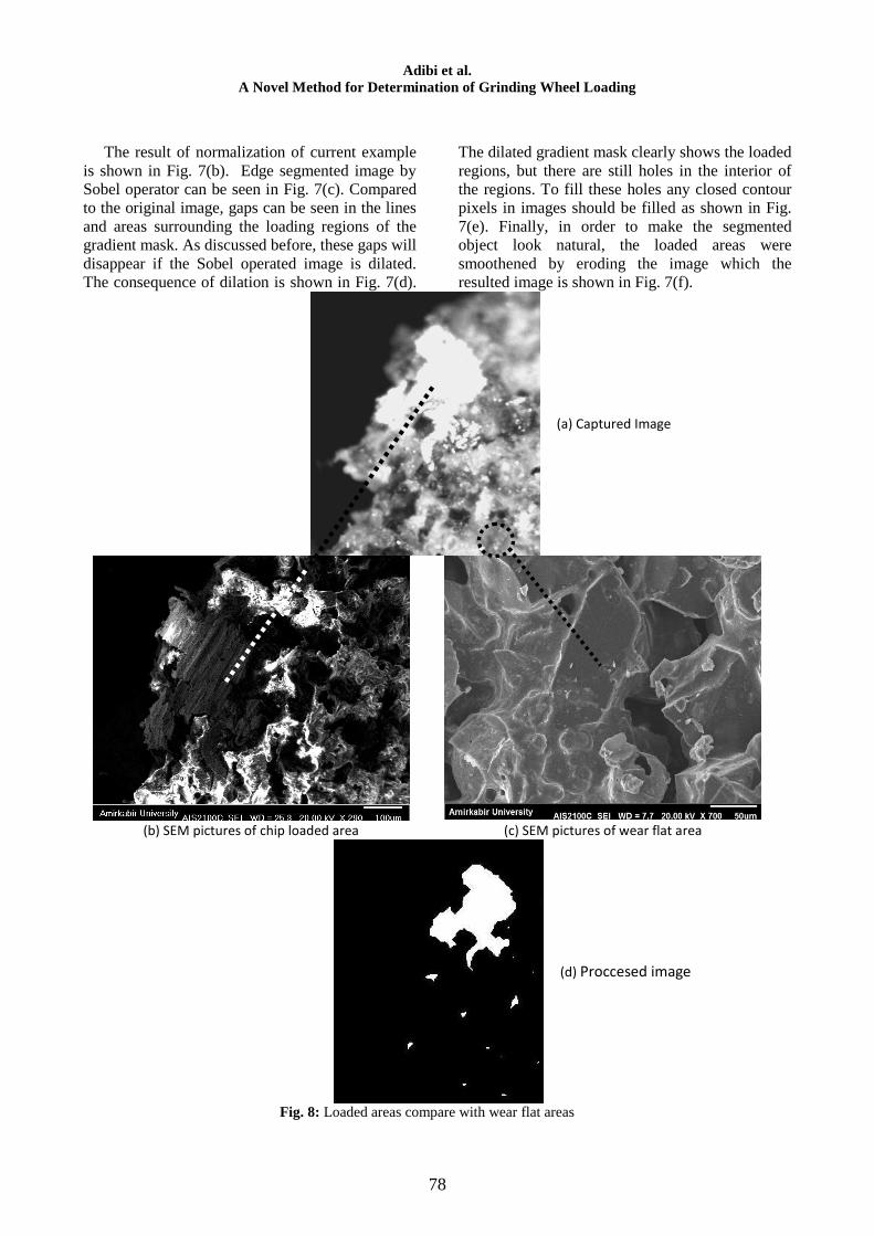
(a) Captured Image

(b) SEM pictures of chip loaded area (c) SEM pictures of wear flat area

(d) Proccesed image

Fig. 8: Loaded areas compare with wear flat areas


79

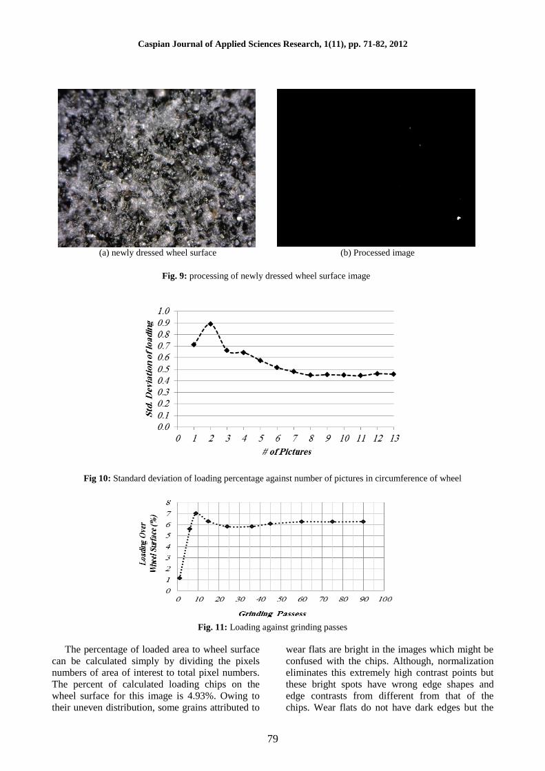
(a) newly dressed wheel surface (b) Processed image

Fig. 9: processing of newly dressed wheel surface image

Fig 10: Standard deviation of loading percentage against number of pictures in circumference of wheel

Fig. 11: Loading against grinding passes

The percentage of loaded area to wheel surface

can be calculated simply by dividing the pixels

numbers of area of interest to total pixel numbers.

The percent of calculated loading chips on the

wheel surface for this image is 4.93%. Owing to

their uneven distribution, some grains attributed to

wear flats are bright in the images which might be

confused with the chips. Although, normalization

eliminates this extremely high contrast points but

these bright spots have wrong edge shapes and

edge contrasts from different from that of the

chips. Wear flats do not have dark edges but the

Adibi et al.


80

loaded areas have dark edges. By applying the

iterative method for thresholding, high bright grain

spots attributed to wear flats and also vitreous bond

can be ruled out. To observe the wheel surface

more clearly, a section of wheel surface was cut

and was observed under SEM. As it can be seen in

Fig. 8, CBN grains seem different from loaded

chips. Figure 8(d) shows the processed image

which does not include the wear flat area. This is

due to different light reflected by CBN. The

iterative method for determination of threshold

value also eliminates the regions attributed to wear

flats.

Figure (9) shows the image of a newly dressed

wheel surface. Figure 9(a) is the original image

and 9(b) is the processed gradient mask image. The

ratio of loading of a fresh wheel surface is

calculated to be 0.0604% in Fig. 9. The error is

less than 0.1% which is acceptable in surface

monitoring for grinding wheels.

To investigate the minimum number of pictures

collected around the wheel circumference and

reach steady state of the standard deviation of the

loading percentage, grinding tests were carried out.

Setup parameters and specification of the grinding

system is presented in Table 1. Positioning

assembly, as mentioned above, traverses the

microscope in the width direction of the wheel.

Four images in each circumferential location were

captured to cover the full width. This process was

done on several circumferential locations.

Numbers of locations at wheel circumference

ranging from three to thirteen were considered.

Each image was processed and average standard

deviations were calculated. In Figure 10 standard

deviation of loading percentage against number of

picture locations are plotted. After eight pictures in

circumference of the wheel, standard deviation

remained constant. Therefore eight locations from

circumference and four images for each location

across the width of the wheel were chosen to

determine the amount of wheel loading.

To investigate the repeatability of the process,

the average and standard deviation of loading

percentage were calculated for different initial

location of image capturing in the wheel

circumference. The results are shown in Table. 2.

A significant change is not seen for each condition.

The steadiness of average value for more than

eight numbers of pictures also shows good

repeatability of the method.

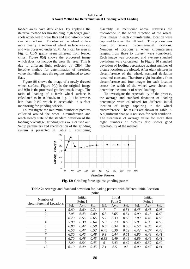
Fig. 12: Grinding force against grinding passes

Table 2: Average and Standard deviation for loading percent with different initial location

point

Number of

circumferential Locations

Initial

Point 1

Initial

Point 2

Initial

Point 3

%L Avr. Std. %L Avr. Std. %L Avr. Std.

1 5.80 5.80 0.71 7 7 0.51 6.45 6.45 0.05

2 7.05 6.43 0.89 6.3 6.65 0.54 5.90 6.18 0.60

3 6.79 6.55 0.66 5.7 6.33 0.68 7.00 6.45 0.55

4 5.90 6.39 0.64 5.9 6.23 0.65 5.95 6.33 0.55

5 6.80 6.47 0.58 6.8 6.34 0.58 6.50 6.36 0.48

6 6.50 6.47 0.52 6.45 6.36 0.52 6.42 6.37 0.43

7 6.30 6.45 0.48 6.9 6.44 0.51 6.80 6.43 0.41

8 6.70 6.48 0.45 6.83 6.49 0.49 6.89 6.49 0.41

9 7.00 6.54 0.45 6 6.43 0.49 6.80 6.52 0.40

10 6.10 6.49 0.45 7.1 6.5 0.5 6.00 6.47 0.41


81

11 6.91 6.53 0.44 6.2 6.47 0.48 6.60 6.48 0.39

12 5.90 6.48 0.46 6.87 6.5 0.48 6.20 6.46 0.38

13 6.90 6.51 0.46 6.35 6.49 0.46 7.00 6.50 0.39

Average Value 6.50 6.49 6.50

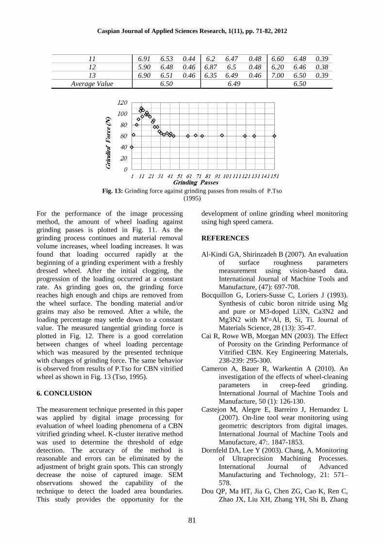
Fig. 13: Grinding force against grinding passes from results of P.Tso

(1995)

For the performance of the image processing

method, the amount of wheel loading against

grinding passes is plotted in Fig. 11. As the

grinding process continues and material removal

volume increases, wheel loading increases. It was

found that loading occurred rapidly at the

beginning of a grinding experiment with a freshly

dressed wheel. After the initial clogging, the

progression of the loading occurred at a constant

rate. As grinding goes on, the grinding force

reaches high enough and chips are removed from

the wheel surface. The bonding material and/or

grains may also be removed. After a while, the

loading percentage may settle down to a constant

value. The measured tangential grinding force is

plotted in Fig. 12. There is a good correlation

between changes of wheel loading percentage

which was measured by the presented technique

with changes of grinding force. The same behavior

is observed from results of P.Tso for CBN vitrified

wheel as shown in Fig. 13 (Tso, 1995).

6. CONCLUSION

The measurement technique presented in this paper

was applied by digital image processing for

evaluation of wheel loading phenomena of a CBN

vitrified grinding wheel. K-cluster iterative method

was used to determine the threshold of edge

detection. The accuracy of the method is

reasonable and errors can be eliminated by the

adjustment of bright grain spots. This can strongly

decrease the noise of captured image. SEM

observations showed the capability of the

technique to detect the loaded area boundaries.

This study provides the opportunity for the

development of online grinding wheel monitoring

using high speed camera.

REFERENCES

Al-Kindi GA, Shirinzadeh B (2007). An evaluation

of surface roughness parameters

measurement using vision-based data.

International Journal of Machine Tools and

Manufacture, (47): 697-708.

Bocquillon G, Loriers-Susse C, Loriers J (1993).

Synthesis of cubic boron nitride using Mg

and pure or M3-doped Li3N, Ca3N2 and

Mg3N2 with M'=Al, B, Si, Ti. Journal of

Materials Science, 28 (13): 35-47.

Cai R, Rowe WB, Morgan MN (2003). The Effect

of Porosity on the Grinding Performance of

Vitrified CBN. Key Engineering Materials,

238-239: 295-300.

Cameron A, Bauer R, Warkentin A (2010). An

investigation of the effects of wheel-cleaning

parameters in creep-feed grinding.


Manufacture, 50 (1): 126-130.

Castejon M, Alegre E, Barreiro J, Hernandez L

(2007). On-line tool wear monitoring using

geometric descriptors from digital images.


Manufacture, 47:. 1847-1853.

Dornfeld DA, Lee Y (2003). Chang, A. Monitoring

of Ultraprecision Machining Processes.

International Journal of Advanced

Manufacturing and Technology, 21: 571–

578.

Dou QP, Ma HT, Jia G, Chen ZG, Cao K, Ren C,

Zhao JX, Liu XH, Zhang YH, Shi B, Zhang

Adibi et al.


82

TC (2006). Light emission from cBN crystal

synthesized at high pressure and high

temperature. Applied Physics Letters, id.

154102, 88(15).

Eremets MI, Gautheir M, Polian A, Chervin JC,

Besson JM (1995). Optical properties of

cubic boron nitride. PHYSICAL REVIEW

B, The American Physical Society, 52: 8854-

8863.

Feng Z, Chen X (2007). Image processing of

grinding wheel surface. International Journal

of Advanced Manufacturing Technology, 32:

27–33.

Gonzalez RC, Woods RE (2010). Digital Image

Processing. Prentice Hall, 2010.

Haines J, Leger JM, Bocquillon G (2001).

Synthesis and design of superhard materials.

Annual Review of Materials Research, 31: 1.

Hosokawa A, Yasui H (2000). Characterization of

the grinding wheel Surface by Means of

Image Processing (1st report). JSPE, 62 (9):

1297–1301.

Kim SH, Ahn JH (1999). Decision of dressing

interval and depth by the direct

measurement. Journal of Materials

Processing Technology, 1999, Vol. 88, pp.

190–194.

Konig W, Lauer-Schmaltz H (1978). Loading of

the wheel phenomenon and measurement.

Annals of the CIRP, 27: 217–220.

Lachance S, Bauer R, Warkentin A (2004).

Application of region growing method to

evaluate the surface condition of grinding

wheels. International Journal of Machine

Tools & Manufacture, 44(7-8): 823–829.

Lauer-Schmaltz, H. ; Konig, W. Phenomenon of

Wheel Loading Mechanisms in Grinding.

Annals of CIRP, 1980, Vol. 29, pp. 201-206.

Liu Q, Xun C, Nabil G (2007). Assessment of

Al2O3 and superabrasive wheels in nickel-

based alloy grinding. International Journal of

Advanced Manufacturing Technology, 940–

951.

Mao C, Zhou ZX, Ren YH, Zhang B (2010).

Analysis and FEM Simulation of

Temperature Field in Wet Surface Grinding,

Materials and Manufacturing Processes,

25(6): 399-406.

Mersmann C (2011). Industrializing metrology—

Machine vision integration in composites

production. CIRP Annals - Manufacturing

Technology, 60: 511-514.

Meyer F (1992). Color image segmentation.

Maastricht, The Netherlands in Proc. Int.

Conf. Image Processing, 303 – 306.

Mokbel AA, Maksoud TMA (2000). Monitoring of

the condition of diamond grinding wheels

using acoustic emission technique, Journal of

Materials Processing Technology, 101(1–3):

292–297.

Nelson S A (2012).

http://www.tulane.edu/~sanelson/geol211.

[Online] Tulane University. [Cited: Feb. 16,

2012.]

Peatross J, Ware M (2011). Physics of Light and

Optics. [ed.] C. online textbook.

Sakamoto H, Shimizu S, Kato D (1998).

Evaluation of Loading Behavior of Grinding

Wheel Based on Working Surface

Topography. Journal of the Japan Society of

Precision Engineering, 64(9): 1320-1324.

Li S, Lijie C, Hao L, et al. (2010). Large Scale

Growth and Characterization of Atomic

Hexagonal Boron Nitride Layers. NanoLett,

10 (8): 3209–3215.

Srivastava AK, Ram KS, Lal GK (1985). A new

technique for evaluating wheel loading.

International Journal of Machine Tools Des.

& Res., 25: 33-38.

Teichera U, Künanz K, Ghosh A, Chattopadhyay

AB (2008). Performance of Diamond and

CBN Single-Layered Grinding Wheels in

Grinding Titanium, Materials and

Manufacturing Processes, 23(3).

Tso PL (1995). Study on the grinding of Inconel

718. Journal of Materials Processing

Technology, 55: 421-426.

Wei J, Zhang Q, Xu Z, Lyu (2010). Study on

precision grinding of screw rotors using

CBN wheel, International Journal of

Precision Engineering and Manufacturing

International Journal of Precision

Engineering and Manufacturing, 11 (5): 651-

658.

Yasui H, Hiraki Y, Sakata M (2001). Development

of Automatic Image Processing System for

Grinding Wheel Surface. J. Japan society

for prec. Eng., 67.

Zhong Z, Hung NP (2000). Diamond Turning and

Grinding of Aluminum-Based Metal Matrix

Composites, Materials and Manufacturing

Processes , Volume 15(6): 853-865.

Zhong Z, Ramesh K, Yeo SH (2010). Grinding of

nickel-based supper-alloys and advances

ceramics, Materials and Manufacturing

Processes, 16 (2): 195-207.

CJASR-12-13-119

Documents

Transcript of CJASR-12-13-119