Christopher Nantista

2011 Linear Collider Workshop of the Americas (ALCPG11)

University of Oregon, EugeneMarch 20, 2011

.…………………….

First, I’d like to offer congratulations to our KEK colleagues on their DRFS development and successful S1-Global work (which I hope we’ll get to hear more about soon), and our prayers for a swift recovery from the impact of recent events.

Ganbatte, Nihon!

Reviewand Developments

KLYSTRON CLUSTER BUILDING

CTOCTO CTOCTO

ACCELERATOR TUNNEL

2.05 km of linac powered per 2-cluster shaft. 12 shafts total for both linacs.

Klystron Cluster Scheme• Main linac rf power is produced in surface buildings and brought

down to and along the tunnel in low-loss circular waveguide.• Many modulators and klystrons are “clustered” to minimize

surface presence and number of required shafts.• Power from a cluster is combined and then tapped off in equal

amounts at 3-cryomodule (RDR rf unit) intervals.

• equipment accessible for maintenance

• tunnel size smaller than for other one-tunnel options

• underground electrical power and heat load significantly reduced

ADVANTAGES

Concepts by Holabird/Root

Two clusters can be housed in one building (feeding upstream and downstream).

10 MW, 1.6 ms MBK’s (multi-beam klystrons) powered by 120 kV RDR or Marx modulators.

An initial low power (bunch number) installation, should include klystrons furthest from the shaft, allowing their combining waveguide circuit to remain intact when more sources are added. This likely requires full size building construction.

KCS Surface Buildings

from Vic Kuchler

KCS Main Waveguide

TE01 mode

30

201

201

200 )/(

1

akakZ

Rs

E

0.480 m (18.90”)

For long distance, high-power rf transmission, use the TE01 mode in circular waveguide.

• No surface electric field → high power handling capacity• Attenuation falls quickly with radius → low loss achievable• Extensive experience from NLC pulse compression, power distribution R&D

WC1890

evacuated or pressurized

Waveguide Diameter (m)

Pow

er A

ttenu

atio

n O

ver

1 km

--- copper--- aluminum

A novel waveguide device was developed for coupling into and out of the circular TE01 mode waveguide without creating large surface fields.

Combining and Distributing Power

CTO (Coaxial Tap-Off)

For combining, the tap-offs are used in reverse.Proper phase and relative amplitude needed for match (mismatched power goes to circulators).

determines coupling

Couplings ranging from ~1 to 1/33 are required.

CTO’s of increasing coupling every ~38 m

C =~1/27 C =~1/26 C =~1/2 C =~1

…

Tunnel Cross-SectionCTO

Replace vacuum windows w/ smaller pressure windows.Eliminate combiner and add two high-power circulators.

Local RF Power Distribution SchemePower from each CTO is distributed along a 3-CM, 26 cavity rf unit through a local PDS. Distribution is tailored to accommodate gradient limits of cavities.

Original VTO (Variable Tap-Off) Pair-Feeding Concept

• manually adjustable by pairs• requires pair sorting• circulators can be eliminated

Alternate Scheme w/ Folded Magic-T’s and Motorized U-Bend

Phase Shifters• remotely adjustable by pairs• requires pair sorting• circulators can be eliminated

Folded Magic-T’s and Motorized U-Bend s for Each Cavity

• remotely adjustable by cavity• no pair sorting required• circulators required

CTOcustomizable

coupler feed 1 feed 2

hybridload

quad

every ~38 m

With 12 rf units* moved from the RTML to each of the main linacs and 4 more in the e- linac to compensate for undulator losses, they have 294 and 290 rf units, respectively.

The following would seem to be a reasonable modified KCS layout.

-- main facilities shaft-- additional KCS shaft

27 27 2727 27 27 27 27 27

e- beam

27

Shafts and RF Units* per KCS

24

27 27 2727 27 27 27 27 272720

e+ beam

undulator

~2.05 km

*rf unit 3 cryomodules = 26 cavities

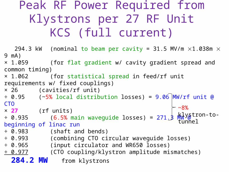
294.3 kW (nominal to beam per cavity = 31.5 MV/m 1.038m 9 mA)× 1.059 (for flat gradient w/ cavity gradient spread and common timing)× 1.062 (for statistical spread in feed/rf unit requirements w/ fixed couplings)× 26 (cavities/rf unit)÷ 0.95 (~5% local distribution losses) = 9.06 MW/rf unit @ CTO× 27 (rf units)÷ 0.935 (6.5% main waveguide losses) = 271.3 MW @ beginning of linac run÷ 0.983 (shaft and bends)÷ 0.993 (combining CTO circular waveguide losses)÷ 0.965 (input circulator and WR650 losses)÷ 0.977 (CTO coupling/klystron amplitude mismatches)

284.2 MW from klystrons

~8% klystron-to-tunnel

Peak RF Power Required from Klystrons per 27 RF Unit KCS (full current)

With 31 klystrons and 30 on, we have 290.3 MW available (2.2% to spare).

However, we also need 7% (5% usable) overhead for LLRF to be harnessed via phase control of the rf drives, oppositely dephased in pairs, such that the combined power is reduced as P = Pmax cos2 f, with f nominally 15˚.

Klystrons Needed per 27 Unit KCS (full current)

However, we want to be robust against a single klystron failure per system. With N sources combined in a passive network, failure of one source leaves combined the equivalent of (N-1)2/N sources.

The calculation/estimate suggests we need 284.2 MW worth of klystron power.At 10 MW each, 29 klystrons would give us 290 MW (2.0% to spare).

The maximum power requirement rises to 284.2 MW ÷ 0.933 = 304.6 MW,

With 33 klystrons and one off, we have 310.3 MW (1.9% to spare).

f -fV2n V2n-1

Vtot

(30 klystrons for the 24 unit KCS and 25 klystrons for the 20 unit KCS)

TOTAL: 20×33 + 30 + 25 = 715 klystrons installed (693 on)

27 Unit KCS Average Power Diagram (full current)

cavity reflection loads

distribution end loads

local distribution waveguide

main KCS tunnel waveguide

shaft & bends

combining waveguide (CTO’s)

klystron waveguides

klystron collector (.65)

modulator (.95)

beam

“wall plug” power supplies (.92)

1.001 MW(31.5MV/m1.038m9mA0.969ms5Hz26cav/unit27units)

4.408

4.055

3.852

2.504

2.416

2.399

2.080

2.044

1.911

1.816

1.710

1.001

combining loads

4.408 MW

353 kW

203 kW

1.348 MW

87.6 kW

17.0 kW

319 kW

35.4 kW

133.2 kW

95.6 kW

105.8 kW

708.8 kW

heat loadsflow (MW)

tunnel

320 MW peakIncludes power mismatched due to spare and overhead misphasing.

beam (~23%)

Reduced Beam Current

( ) 11/

2ln2 −⎥⎦

⎤⎢⎣

⎡−+=+=

==

BBce

birf

Bcecbrf

fnVQeRN

ttt

feVNVIP

ω

Halving the number of bunches in the ILC beam pulse is adopted as a way to reduce the initial cost of the machine. The direct impact on the luminosity is ameliorated by introduction of a traveling focus scheme. In this reduced beam current “low power” scenario, site power is reduced, along with water cooling requirements.

Additionally, for the high-power rf system, the amount of installed rf production equipment can be significantly reduced.

The impact depends on the bunch frequency, fB, which affects:

beam pulse current: Ib = Nee fB

beam pulse duration: tb = (nB – 1) fB-1

rf power per cavity:

rf pulse duration:

and thus

KCS Low PowerKCS is very flexible. Combining tens of klystrons allows us to adjust installed power with relatively fine granularity.

Simply eliminating every other bunch (halving fB) maintains the beam duration and halves the current, cutting in half the required peak power. However, it also doubles the cavity fill time. , thereby increasing the required rf pulse width at full gradient by 38%.

It’s preferable to adopt parameters which allow use of the modulators and klystrons developed for full RDR beam specifications, i.e. to stay within the ~1.6 ms pulse width. This can be achieved by reducing the bunch spacing to increase the current to 0.69 I0. The rf peak power required at the cavities is reduced from that for the full beam by this factor.

Fixed tb:

Fixed trf:

beamfill

-- full beam-- ½ current-- retains rf pulse width

(Prf → ½ Prf0, trf → 1.38 trf0)

(Prf → 0.69 Prf0, trf → trf0)

With 22 klystrons and 21 on, we have 200.5 MW available (2.2% to spare).

However, we also need 7% (5% usable) overhead for LLRF to be harnessed via phase control of the rf drives, oppositely dephased in pairs, such that the combined power is reduced as P = Pmax cos2 f, with f nominally 15˚.

Klystrons Needed per 27 Unit KCS (1/2 bunches)

However, we want to be robust against a single klystron failure per system. With N sources combined in a passive network, failure of one source leaves combined the equivalent of (N-1)2/N sources.

Scaling from the full current case, we need (0.69×284.2=) 196.1 MW worth of klystron power. At 10 MW each, 20 klystrons would give us 200 MW (2.0% to spare).

The maximum power requirement rises to 196.1 MW ÷ 0.933 = 210.2 MW,

With 23 klystrons and one off, we have 210.4 MW (0.12% to spare).

f -fV2n V2n-1

Vtot

(21 klystrons for the 24 unit KCS and 18 klystrons for the 20 unit KCS)

TOTAL: 20×23 + 21 + 18 = 499 klystrons installed (477 on) 30.2% reduced from full current

bb

cbirf

cbrf

tI

V

QRttt

VIP

+=+=

=

/2ln2

ω

RDR-Like Fallback Low PowerWith the KCS and DRFS schemes in development, an RDR-like layout w/ 10 MW klystrons, modulators, etc. in the (enlarged) single tunnel is considered the fallback plan.

For half bunches operation, one could double the bunch spacing and install half the modulators and klystrons, each feeding 6 CM’s, rather than 3.

This would double the fill time, increasing the required rf pulse width by 38%.The installed modulators and klystrons would then be overspec.ed for the upgrade.

FULL BEAM

HALF BEAM

Prf → ½ Prf0

trf → 1.38 trf0 every other klystron omitted

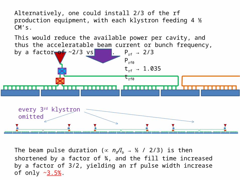
Alternatively, one could install 2/3 of the rf production equipment, with each klystron feeding 4 ½ CM’s.

This would reduce the available power per cavity, and thus the acceleratable beam current or bunch frequency, by a factor of ~2/3 vs. RDR.

The beam pulse duration ( nB/Ib → ½ / 2/3) is then shortened by a factor of ¾, and the fill time increased by a factor of 3/2, yielding an rf pulse width increase of only ~3.5%.

every 3rd klystron omitted

Prf → 2/3 Prf0

trf → 1.035 trf0

250 GeV/beam

# of bunches

bunch spacing

beam current

beam duration

rf peak power

fill time, ti

rf pulse duration

full beam 2625 369.2 ns 9 mA 0.969 ms 294.2 kW 0.595 ms 1.564 ms

½ bunches A 1313 738.5 ns 4.5 mA 0.969 ms 147.1 kW 1.190 ms 2.159 ms (up 38%)

½ bunches B KCS

1313 535.1 ns 6.21 mA 0.702 ms 203.0 kW 0.862 ms 1.564 ms

½ bunches B RDR

1313 553.8 ns 6 mA 0.727 ms 196.1 kW 0.893 ms 1.619 ms (up 3.5%)

-- full beam 0%-- ½ bunches A 40.6%-- ½ bunches B (KCS) 1.9%-- ½ bunches B (RDR) 5.5%

@ 31.5 MV/m cryo load increase*

* Only includes dynamic load of fundamental rf in cavity. Additional contributions come from coupler (linear w/ power and time) and HOM (current dependent).

Parameter Summary

Parameter choice also impacts cryogenic load.

Installation for Reduced BunchesKCS:• Everything in the tunnel is installed.• 69.8 % (499/715) of high power rf production equipment (klystrons,

modulators, power supplies, etc.) in KCS surface buildings, upstream from shaft, with main waveguide runs traversing the region where the rest will go.

• 68.8% (477/693) of “wall plug” power for main linac high power rf.• 75%* of water cooling capacity for heat load from high power rf.

RDR-Like Fallback:• 66.7 % of high power rf production equipment in the linac tunnels,

with additional power dividers and waveguide.• 69% (1.035 × 2/3) of “wall plug” power for main linac high power rf.• ~ 75%* of water cooling capacity for high power rf heat load.

HPRF heat load distribution (from slide 12):above ground – 68.3%below ground – 31.2% (65.7% fixed, 34.3% power dependent)

HPRF heat load reduction factor:above ground – 0.69below ground – (0.657 + 0.343×0.69) = 0.894Total – (0.683×0.69 + 0.312×0.894 ) = 0.750

-- full beam-- ½ bunches A-- ½ bunches B (KCS)-- ½ bunches B (RDR)

Heat Load Breakdown for KCSThe rf energy deposited per pulse into the cavity reflection loads (circulator loads), being the product of Prf (Ib) and ti (Ib

-1),is, for a given gradient, constant across the parameter sets.

For the RDR-like layout the total reduction is the same, 0.75, all below ground.

Transition to Full Beam CurrentKCS:• Upgrade is all above ground.• Install remaining 31% of “wall plug” power capacity.• Install remaining 25% of cooling capacity.• Install remaining 30.2% of high-power rf hardware in the KCS

buildings. Most, up to the point of connecting the sources into the main waveguide, can be done while running.

RDR-Like Fallback:• Install remaining 31% of “wall plug” power capacity.• Install remaining 25% of cooling capacity.• Install remaining 33.3 % of high-power rf hardware in the linac tunnels.

ILC is shut down during installation.

Low ECM OperationAnother design change was the relocation of the undulator for e+ production from the middle to the end of the e- linac, closer to the damping rings. This poses a problem.

For sufficient positron production, the e- beam needs to be @ 150 GeV.

The physics specifications for the ILC call for running at various center-of-mass energies:

500 GeV, 350 GeV, 250 GeV, 230 GeV, and 200 GeV.

Previously, for the operation points < 300 GeV c.o.m., the e- beam could be decelerated from 150 GeV after the undulator; with the undulator at the end, it can’t be.

Solution:For 250 GeV c.o.m. and below, run e- linac at double rep. rate, 10 Hz, alternating between 150 GeV pulses for e+ production and half the desired ECM for collisions.

To retain luminosity for ECM ≤ 250 GeV (≤125 GeV/beam), run e- linac (only) @ 10Hz, alternating between 150 GeV for e+ production and the desired collision energy.

In this scheme, because the cavity couplers are mechanical, QL cannot be optimized for both gradients, but is set for the 150 GeV gradient (150/250 × 31.5 MV/m = 18.9 MV/m).

For flat gradient during the alternating lower cavity voltage (VL) pulses the needed input power and the residual cavity reflection (during the beam) are given by:

PL = ¼ (1 + VL/V150)2 P150 = 0.8403, 0.7803, 0.6944 P150 @ 125, 115, 100 GeV

Pr = ¼ (1 VL/V150)2 P150 = 0.694%, 1.36%, 2.78% P150 @ 125, 115, 100 GeV

Fill: const. power, PL,

OR

const. fill time, ti, PLi = (VL/V150)2 P150

( )i

LiL t

VVt

2ln

/1ln 150+= = 0.8745, 0.8210, 0.7370 ti150 @ 125, 115, 100 GeV

= 0.6944, 0.5878, 0.4444 P150 @ 125, 115, 100 GeV

To fill the cavity by beam arrival, one must also either toggle the timing or step the power level during the pulse (between fill and beam).

10 Hz Running Considerations

or

Ib = KVa3/2,

Pmod = IbVa = KVa

5/2

SLAC/KEK Toshiba 10 MW MBK

For 125 GeV beam, one needs 5 MW per tube (vs. 10 MW for 250 GeV), Vmod can be lowered from 117 kV to 94 kV, reducing modulator peak power to (94/117)5/2 = 0.579 × the nominal value.Also, pulse width is reduced by a factor of [(125/250)×.595ms + .969ms]/1.564 ms = 0.810 pulse energy reduced by factor of ~0.469.

For the 150 GeV pulses, Vmod = 99.5kV, and this factor becomes .667×.848 = 0.565, and for the alternate 125 GeV pulse .579 ×.819 = 0.474

So the power load factor for the e- linac running at 10 Hz is about 0.565 + 0.474 = 1.039, a slightly increased demand. This can be avoided by running at 9.6 Hz, instead. For both linacs combined, the HLRF power load is downby (1.039 + 0.469)/2 = 0.754.

Impact on Power Requirements

(e+ linac)(e- linac)

At lower gradients, reduce modulator voltage and increase pulse rate so that nominal average modulator input power not exceeded. → charging power supplies would see the same or smaller load (which is roughly constant), and the AC power capacity would not have to be increased.

Effect on Modulator Charging

Discharge less energy per pulse at increased rep rate.

Time

Mod

ulat

orCe

ll Vo

ltage

Same Slope Discharge Level Differs Every Other Pulse5 Hz 10 Hz

Additional line ripple introduced by alternating discharge levels would need to be reduced in the site electrical distribution system.

R & D

Marx Modulator and Toshiba MBK Operation

Blue: no droop compensationGreen: with only delay cells Red: with delay cells and Vernier

The Toshiba 10 MW MBK is being run into loads for lifetime testing while itself providing a load for testing of SLAC’s 120kV, 140A, 1.6 ms, 5Hz Marx modulator.

SLAC P2 Marx: Progress Highlights*

Cell Output CurrentCell Output VoltageMain IGBT Vce

PWM Inductor Current

Demonstrated Active Droop Compensation Scheme

Load CurrentMain IGBT Vce

Load Voltage

Demonstrated FaultTolerance

loadarc

140A @ 4kV

PWMcurrent

* from Mark Kemp

A second generation Marx modulator is in development at SLAC.

SLAC P2 Marx: Progress Highlights• Primary progress to-date at cell level

• All hardware has been prototyped• Controls firmware has been written, but is not in final form• All cell fabrication drawings have been finalized• Cell has been tested in (nearly) all anticipated operating scenarios

(nominal, fault, peak power, peak cell voltage, peak output average power, operation into stiff current source)

• Full modulator quantities of cells are currently being fabricated• >95% farmed out to industry• All in-house by end of April• Final assembly at SLAC9-10 feet (2.8 – 3.1 m)

4-5 feet(1.2 – 1.5 m)

• Overall modulator status• Modulator being assembled• Able to hold cells mid-April• Start of full modulator testing by June.• Application manager software undergoing

updates with final implementation to be in EPICS.• Design aspects

• Single side access• No oil• No transformer• N+2 redundancy /w automatic reconfiguration• Active correction scheme• Cell diagnostic and prognostic capability

• Modulator Height: 7-8 feet (2.1 – 2.4 m)• Located separately is double-bay power supply

rack• Cells are air cooled. Heat is removed via

air/water heat exchanger.

U-bend Phase Shifter for Local Power Tailoring in PDS

A folded magic-T provides convenient port orientations.

1 2

3

Cavity-to-cavity spread in sustainable gradient make it desirable to be able to tailor the local power distribution along the cryomodules.

The VTO allowed manually-set fixed tailoring to matched pairs of cavities.

As a more flexible alternative, a pressurizable U-bend phase shifter with motor-controlled feed through was developed, for use in pairs between folded magic-T’s.

Opposite phase adjustment varies the split at ports 2&3, without changing the output phases.

(in-line phase shifters still used to adjust phase at cavity couplers)

U-bend Phase Shifter Testing

max reflection: ~0.025% (-36 dB)

mean loss: ~0.51% (-.0221 dB)

No breakdowns were detected during 8 hours running in 1bar N2 @ 2MW.

Cold

Tes

tH

ot T

est

Eight such phase shifters have been fabricated for the second PDS for Fermilab’s NML facility. The first 2-feed PDS module is ready for testing.

Fully Adjustable PDSFor ILC, w/ large (±20%) gradient limit spread, individual cavity adjustment of the power division can be achieved via the below PDS layout.Cost and power losses will be increased, however, over pair-wise division due to doubling the number of power division units and including circulators.

CTO (Coaxial Tap-Off)

A pair of 3-dB CTO’s.

A CTO connecting WR650 waveguide to 0.48 m-diameter circular waveguide.

0.349 m

Inner view showing wrap-around slots.

CTO Cold Test

@1.300 GHz:R = -20.43 dB (0.906%)T = -0.0843 dB (98.08%)

@1.3036 GHz:R = -27.84 dB (0.164%)T = -0.0421 dB (99.04%)

red – reflectionblue – transmissionyellow – loss

We tested our CTO’s as back-to-back launchers:

This initial test indicates good performance of the CTO’s, the 36 MHz offset of the optimum being attributable to deliberate endcap undermachining (for intended shim tuning and remachining). Further tests with a ¼-wave spacer were deferred for schedule reasons.

Shorting one circular port of a 3dB CTO at the proper distance, converts it into a mode launcher (or partial coupler).

launcher coupler

for resonant testfor transmission test

Klystron Cluster Scheme TestsResonantly power a 10 m long 0.48 m diameter aluminum pipe,

pressurized (1atm N2), to 300 MW TE01 mode field equivalent, in 1 ms pulses.

No Breakdown for more than 50 hours

550 kW input corresponds to 75 MW traveling waves, creating a standing-wave pattern with peak fields equivalent to 300 MW one way.

Faya Wang

Time of Position 2 markers (T1,T2) are ~ 1 ms later than those from Position 1, which suggest events are much closer to Position 1 (5 m / 5100 m/s ~ 1 ms) T1 T2

Acoustic Sensor Breakdown Localization

CTO 21

550 KW input power yields 300 MW equivalent surface fields in the pipe - see bkdn every ~ 15 hours, maybe from CTO or upstream – rate seems very pressure dependent

‘Big Pipe’ Operation

Problem believed to have been waveguide switch near klystron.Further testing is underway.

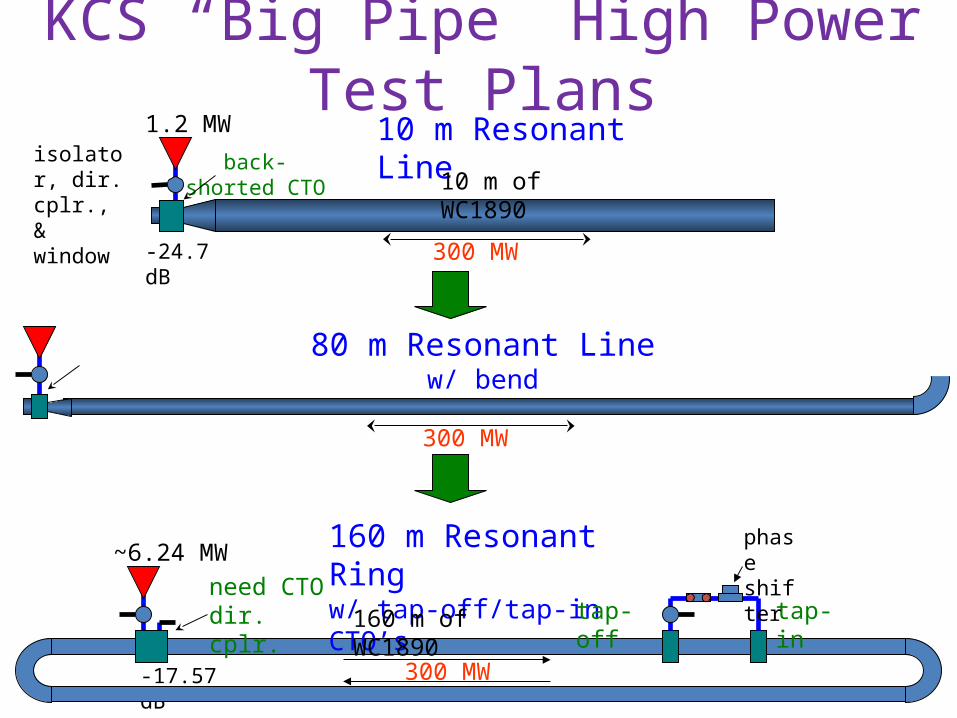
10 m Resonant Line1.2 MW

300 MW-24.7 dB

10 m of WC1890back-shorted

CTO

160 m Resonant Ringw/ tap-off/tap-in CTO’s

~6.24 MW

300 MW-17.57 dB

160 m of WC1890need CTO dir. cplr. tap-off tap-in

phase shifter

80 m Resonant Linew/ bend

isolator, dir. cplr., & window

300 MW

KCS “Big Pipe” High Power Test Plans

“Big Pipe” Resonant Ring LayoutIn End Station B

G. Bowden

Cooling added for phase stability

90˚ Bend for KCS Main Waveguide

1.73 m @ L-band

@ 300 MW: |Es

max| = ~3.684 MV/m |Hs

max| = ~8.377 kA/m|S21|2 = 99.69% (w/o wall losses)Highest parasitic excitation: -28.1 dB

~1.04 m

Complicated taper requires wire e.d.m. of 10.4”-thick aluminum.

SLAC X-band TE01 bend:

Tantawi, Dolgashev, Nantista

For KCS, we need to bend the main rf waveguide at full power through multiple 90˚ bends to bring it down to and along the linac tunnel. Demonstration of such a bend is crucial to establishing the feasibility of KCS.

Our best option seems to be a scaled, modified version of the current standard SLAC bend used in X-band work. Multi-stage linear cross-section tapers convert the circular TE01 mode into the rectangular TE20 mode, which is preserved through a swept bend.

Scaled w/ simplified mid-section

A mechanical design/fabrication plan for this bend is in underway.Optimization of a possible alternate design is being simultaneously pursued.

D=0.3348 m

Compact U-bend version for resonant ring

Summary: Responses to Changes(for KCS option)

Single Tunnel Main Linacs:

KCS - surface buildings, shafts, large waveguide, & CTO’s

±20% Gradient Spread:

overhead for spread in PDS feed requirements

local power division (remotely) controllable by cavity?

Low Power (half bunches):

adjust bunch spacing to maintain rf pulse width

reduced initial installation of rf sources (same building size?)

reduced electrical and cooling requirements

Undulator Relocation:

10 Hz operation of e- linac for low ECM runs to maintain e+ production