Christof Douma

Functional Reactive Programming

What are reactive systems?Transformational vs. Reactive

● Transformational systems compute output from an input and then terminate. Examples: UUAG, GHC, Latex.

● Reactive systems respond to stimuli in order to bring about desirable effects in their environment. Examples: Proxima, Mozilla, Quake, Space Invaders.

Why Functional Reactive Programming?

● Functional programming has usually been applied to build transformational systems.

● Usually imperative paradigms are adopted when building reactive systems.

● FRP is a new paradigm to program reactive systems in a functional language.

● Useful for Embedded Domain Specific Languages

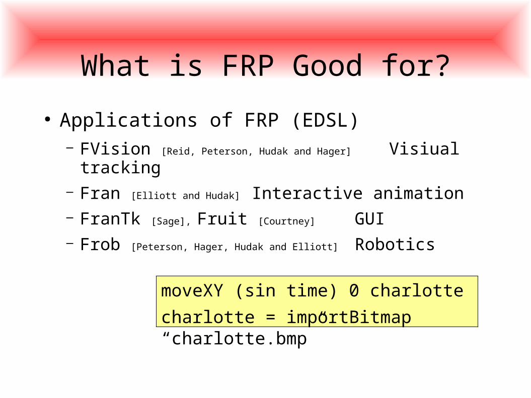
What is FRP Good for?

● Applications of FRP (EDSL)– FVision [Reid, Peterson, Hudak and Hager] Visiual tracking– Fran [Elliott and Hudak] Interactive animation– FranTk [Sage], Fruit [Courtney] GUI– Frob [Peterson, Hager, Hudak and Elliott] Robotics

moveXY (sin time) 0 charlotte

charlotte = importBitmap “charlotte.bmp”

FRP Pardigm

● FRP has two key abstractions● Continuous time-varying values● Discrete streams of events

● Uses combinators that hide detail about timing and synchronization

Signal a = Time -> a

Signal Functions

● Signals can be manipulated directly● Problem: Time- and space-leaks

– Time leaks occur in real-time systems when a computation does not “keep up” with the current time, this requiring “catching up” at a later time.

● Solution: Use Signal Functions– Signals are not fist class values anymore

SF a b = Signal a -> Signal b

Signal Function Example

● An example, the sin function: Floating a => SF a a

time

time

Composing FRP programs

● Complex programs can be build by composing simpler programs

● Current implementation uses the Arrow class– change of name: AFRP

arr :: (a -> b) -> SF a b

(>>>) :: SF a b -> SF b c -> SF a c

first :: SF a b -> SF (a,c) -> SF (b,c)

AFRP Example

● Travel returns a SF that generates a constant signal v while the distance d hasn't yet been travelled.

travel :: Distance -> Velocity -> SF Velocity Velocity

travel d v = integral >>> arr (\d2 -> if d2 < d then v else 0)(note the lack of explicite time)

Composing AFRP programs

● more Arrow combinators

second :: SF a b -> SF (c,a) (c,b)

(<<<) :: SF b c -> SF a b -> SF a c

(&&&) :: SF a b -> SF a c -> SF a (b,c)

(***) :: SF a b -> SF c d -> SF (a,c) (b,d)

loop :: SF (a,c) (b,c) -> SF a b

Arrows vs Monads

● IO Programs are a composition of actions with the details of the state are hidden from the user. It is ran at the top level by an interpreter

● AFRP programs is a composition of signal function with the details of the signals hidden from the user. It is ran at the top level by an interpreter

● Monads composition must be linear● Arrows composition is not linear

AFRP Primitive Signal Functions

identity :: SF a a

constant :: n -> SF a b

integral :: SF Double Double

derivative:: SF Double Double

time :: SF a Time

arr2 :: (a -> b -> c) -> SF (a,b) c

Discrete Events

● Events can be user input as well as domain-specific sensors, interrupts, etc.

● Events are represented as signals of the Event datatype

Event a = NoEvent | Event a

edge :: SF Bool (Event ())

hold :: SF (Event a) a

Discrete events (2)

● Operations on event streams include– mapping, filtering, merging, etc.– Switching of reactive behavior (next slide)

tag :: Event a -> b -> Event b

mergeBy :: (a->a->a) -> Event a -> Event a -> Event a

accum :: a -> SF (Event (a->a)) (Event a)

after :: Time -> b -> SF a (Event b)

repeatedly :: Time -> b -> SF a (Event b)

Switching

● read as: 'Behave as sf1 until the first event in es occurs. Then bind the event value to e and behave as sf2.'

● Note: The time flow restart when switch is made into the new SF.

switch :: SF a (b, Event c) -> (c -> SF a b) -> SF a b

sf1 && es `switch` (\e -> sf2)

Switch Example

travel :: Distance -> Velocity -> SF Velocity Velocitytravel d v = switch (constant v &&& wayTooFar) (\_ -> constant 0)

where wayTooFar = integral >>> arr (>=d) >>> edge

switch :: SF a (b, Event c) -> (c -> SF a b) -> SF a b

(&&&) :: SF a b -> SF a c -> SF a (b,c)

Arrow Syntax

travel d v = forward `switch` stopwhere

stop _ = contant 0forward = proc iv -> do

td <- integral -< ive <- edge -< (td >= d)returnA -< (v,e)

● Preprocessor translate arrow symtax into Haskell with first, arr, (<<<) and loop Arrow operators

Switch Semantics

● Two questions arise about switching semantics:– Does the switch happen exactly at the event time, or

infinitesimally after?– Does the switch happen just for the first event, or for

every event in an event stream?

switch, dSwitch :: SF a (b, Event c) -> (c -> SF a b) -> SF a b

rSwitch, drSwitch :: SF a b -> SF (a, Event (SF a b)) b

Recursive Signal Functions● Suppose incrVel :: SF RobotInput (Event ()) generates

'commands' to increments the velocity of a robot.● concider:

vel :: Velocity -> SF RobotInput Velocityvel v0 = proc inp -> do

rece <- incrVel -< inpv <- drSwitch (constant v0) -< (inp, e `tag`

constant (v+1))returnA -< v● Note that vel is recursively defined, which requires:

– The use of the rec keyword– The use of a delayed switch (drSwitch)

Running the program

● To execute a program we need to connect the SF to the outside world

● Approximate the Continuous-time model

reactimate :: IO (DTime,a) -- sense-> (b -> IO ()) -- actuate-> SF a b-> IO ()

AFrob

Programming Robots with AFRP

AFrob

● AFRob is an EDSL - written in AFRP - for programming robots. It includes a robot simulator.

● AFRob models robots with two wheels and two independent motors. These are called SimBots.

● Each SimBot has a bumper switch, a range object finder, an animate object tracker.

● Each SimBot is controlled by a Signal Function

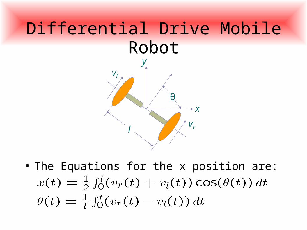
Differential Drive Mobile Robot

θ

l

vl

vr

y

x

● The Equations for the x position are:

Simbot X position

● Assume that:

xSF :: SF SimbotInput DistancexSF = proc inp -> do vr <- vrSF -< inp vl <- vlSF -< inp theta <- thetaSF -< inp i <- integral -< (vr+vl) * cos theta returnA -< (i/2)

vrSF,vlSF :: SF SimbotInput SpeedthetaSF :: SF SimbotInput Angle

● we can write x(t) in AFRP as:

Robot Input Signals

class HasRobotStatus i wherersBattStat :: i -> BatteryStatusrsStuck :: i -> Bool

class HasOdometry i whereodometryPosition :: i -> Position2odometryHeading :: i -> Heading

instance HasRobotStatus SimbotInputinstance HasOdometry SimbotInput

Robot Output Signals

class MergeableRecord o => HasDiffDrive o whereddBrake :: MR oddVelDiff :: Velocity -> Velocity -> MR oddVelTR :: Velocity -> RotVel -> MR o

class MergeableRecord o => HasTextConsole o wheretcoPrintMessage :: Event String -> MR o

mrFinalize :: MergeableRecord o => MR o -> omrMerge :: MergeableRecord o => MR o -> MR o -> MR o

instance HasDiffDrive SimbotOutputinstance HasTextConsole SimbotOutput

Robot Properties

class HasRobotProperties i whererpType :: i -> RobotTyperpId :: i -> RobotIdrpDiameter :: i -> LengthrpAccMax :: i -> AccelerationrpWSMax :: i -> Speed

instance HasRobotProperties SimbotProperties

● Static information about the capabilities of a robot

Robot Controllers

Type SimbotController = SimbotProperties -> SF SimbotInput

SimbotOutput

rcStop :: SimbotControllerrcStop rps = constant (mrFinalize ddBrake)

rcBlind :: SimbotControllerrcBlind rps =

let max = rpWSMax rpsin constant (mrFinalize $ ddVelDiff (max/2)

(max/2))

● A stationary simbot:

● A simbot that goes at ½ of the maximum speed:

Running in Circles

rcTurn :: Velocity -> SimbotControllerrcTurn vel rps = let

vMax = rpWSMax rpsrMax = 2 * (vMax – vel) / rpDiameter rpsin constant (mrFinalize $ ddVelTR vel rMax)

● A simbot that goes at ½ of the maximum speed:

● Simbots cannot turn arbitrarily fast – it depends on their speed. The maximum rotational velocity is:

Another Example Robot Controller

rdDumb :: RobotControllerrcDumb rps = proc sbi -> do

iAmStuck <- rsStuck -< sbirec let sig = (sbi, iAmStuck `tag` constant (-

velo)) velo <- drSwitch (constant maxVel) -< sigreturnA -< mrFinalize $ ddVelDiff velo velo

where maxVel = rpWSMax rps

drSwitch :: SF a b -> SF (a,Event (SF a b)) btag :: Event a -> b -> Event b

● A simbot which reverses when hitting something

Running in a Virtual World

runSim :: Maybe WorldTemplate -> -- virtual world SimbotController -> -- simbot A’s SimbotController -> -- simbot B’s IO () -- does the work

type WorldTemplate = [ObjectTemplate]data ObjectTemplate =

OTBlock { otPos :: Position2 } -- Square obstacle | OTVWall { otPos :: Position2 } -- Vertical wall | OTHWall { otPos :: Position2 } -- Horizontal wall | OTBall { otPos :: Position2 } -- Ball | OTSimbotA { otRId :: RobotId, -- Simbot A robot otPos :: Position2, otHdng :: Heading } | OTSimbotB { . . . } -- Simbot B robot

Demo Programmodule MyRobotShow whereimport AFrob -- AFrob libraryimport AFrobRobotSim -- the simulator

main :: IO ()main = runSim (Just world) rcA rcB

world :: WorldTemplateworld = ...

rcA, rcB, rcB1, rcB2:: SimbotControllerrcA = ... -- controller for simbot A’s

rcB rProps = case rpId rProps of -- controller for simbot B’s 1 -> rcB1 rProps -- (showing here how to deal 2 -> rcB2 rProps -- with multiple simbots)

● where r is the range-finder reading, d is the desired distance, and K

p and K

d are the

proportionate and derivative gains, respectively.

Follow the Wall

● To follow a wall, we use a range finder to sense the distance to the wall.

● It can be shown (for small deviations) that the rotational velocity should be:

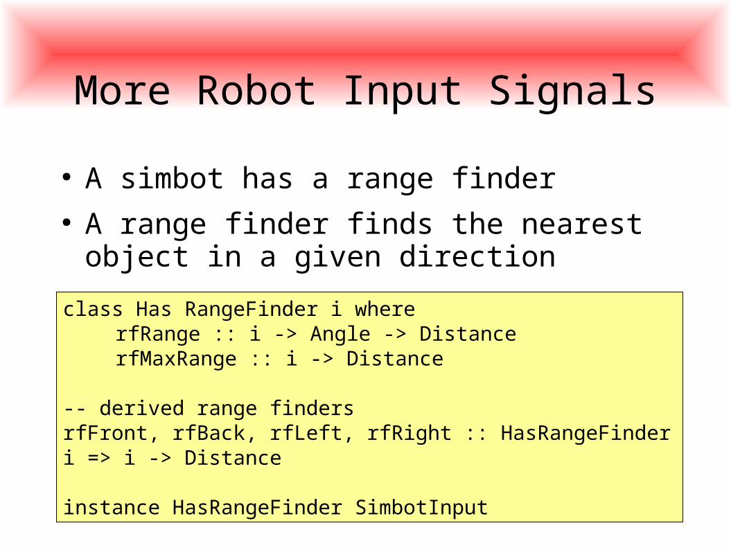
More Robot Input Signals

class Has RangeFinder i whererfRange :: i -> Angle -> DistancerfMaxRange :: i -> Distance

-- derived range findersrfFront, rfBack, rfLeft, rfRight :: HasRangeFinder i => i -> Distance

instance HasRangeFinder SimbotInput

● A simbot has a range finder● A range finder finds the nearest object in a given

direction

Follow the Wall Controller

● This leads to the controller:

rcFollowLeftWall :: Velocity -> Distance -> SimbotControllerrcFollowLeftWall v d _ = proc sbi -> do let r = rfLeft sbi dr <- derivative -< r let omega = kp*(r-d) + kd*dr kd = 5 kp = v*(kd^2)/4 -- achieves “critical damping” returnA -< mrFinalize (ddVelTR v (lim 0.2 omega))

Systems with Dynamic Structure

● All objects are Signal Functions

● Objects can be added and removed

● We need combinators that can change the signal network at runtime

– So far we modelled systems where the signal network is static

Dynamic Collections in AFRP

● AFRP has special combinators for this purpose

parB :: Functor col => col (SF a b) -> SF a (col b)

par :: Functor col => (forall sf.(a->col sf->col (b,sf)))-> col (SF b c) -> SF a (col c)

pSwitch :: Functor col => (forall sf.(a->col sf->col (b,sf)))

-> col (SF b c) -> SF (a,col c) (Event d)-> (col (SF b c) -> d -> SF a (col c))-> SF a (col c)

Learn more?

● Look at the webiste– http://www.haskell.org/yampa/– http://www.haskell.org/frp/

● example application– The Yampa Arcade [Antony Courtney, Henrik Nilsson and John

Peterson, 2003]

– Robot Soccer (included in the yampa package)