Child poverty in Japan: comparing the accuracy of … poverty by consumption < poverty by income?...

Child poverty in Japan:

comparing the accuracy of alternative

measures

Oleksandr Movshuk

Department of Economics,University of Toyama, Japan

[email protected]

Workshop on the Use of Micro-data from Official Statistics,

Institute of Statistical Mathematics, Tokyo

November 21, 2014

Outline

1 Motivation

2 Data and definitions

3 Child poverty rates by income and consumption

4 Why poverty by consumption < poverty by income?

5 Tests for an accurate poverty measure

6 Conclusion

2 /33

Motivation

Alternative resource measures of poverty

Poverty can be evaluated with different resourcemeasures, such as:

Disposable incomeConsumption (either total expenditures or only non-durableexpenditures)Net worth

Income continues to be the most often used measure of

poverty

But for several reasons, consumption may be a better

measure of poverty

3 /33

Motivation

Advantages of using consumption as a poverty

measure

Theoretical advantage

According to the permanent-income hypothesis, it is consumption that

reflects the life-long resources of households. With short-term income

shocks, households could smooth-out their consumption by borrowing.

Income in this case would underestimate the true living conditions

Practical advantage

Compared with income, consumption could have a smaller

measurement error, especially among poor households (Meyer and

Sullivan (2012a, 2012b), Brewer and O’Dea (2012))

4 /33

[email protected]

Motivation

Related literature I

Cutler and Katz (1992, 1993) draw attention to the

conceptual advantages of consumption for measuring

poverty

Using the U.S. household data, they discovered that the

poverty rate with consumption was lower than poverty

rates with income

The finding has been repeatedly replicated for:

the United States (Meyer Sullivan (2012b))the United Kingdom (Brewer et al. (2006))Canada (Brzozowski and Crossley (2011))Japan (Ohtake, Kohara (2011,2013))

5 /33

Motivation

Related literature II

To explain the lower rates of consumption-based poverty,three possible explanations were proposed in theliterature (Meyer, Sullivan (2012b), Brewer et al. (2013)):

1 Under-reporting of incomes (which would inflate thenumber of income-poor households)

2 Over-reporting of consumption expenditures (which wouldreduce the number of consumption-poor households)

3 Use of financial assets or debt to smooth householdconsumption in response to negative income shocks. If thisexplanation is correct, households should run down theirfinancial assets, or add new debts

6 /33

Motivation

Related literature III

Meyer, Sullivan (2012b) and Brewer et al. (2013)

examined these possible explanations with the U.S. and

U.K. data, respectively, and found empirical support for

the first explanation (i.e., income under-reporting)

For Japanese data, Ohtake and Kohara (2011,2013)

mentioned the possibility of consumption smoothing

among poor households, but did not examine the

explanation empirically

In this paper, I will compare child poverty rates in Japan

according to income and consumption, and examine

which of these measures is superior for identifying

materially-disadvantaged children

7 /33

Data and definitions

Data

I used household data from the National Survey of Family

Income and Expenditure (NSFIE)

The survey collects data from a representative sample of

around 50,000 Japanese households

Data include detailed information on household members,

their income sources, numerous expenditure categories,

the stock and flow of household balance sheets, etc., etc.

Probably, the most detailed household survey in the world

I used data from 4 waves of the NSFIE (1989, 1994, 1999,

and 2004)

8 /33


Sample size

Table: Change in the sample size with data cleaning

1. Original sample size 192,599

2. Less: households, marked for unreliable income information 189,107

3. Less: households with negative income or consumption 189,036

4. Less: households with zero income or consumption 189,035

5. Less: household with married household head, younger than 20 years old 188,679

9 /33


Variables and definitions

Resource measures1 Disposable income (total income from all sources less taxes

and social security contributions)2 Total consumption expenditures3 Non-durable consumption (i.e., total consumption less

durable categories)

Child poverty rate was the share of children who lived

below the poverty line

Poverty line was 50% of median equalised

income/consumption

The equivalence scale was the square root of household

size

10 /33

Child poverty rates by income and consumption

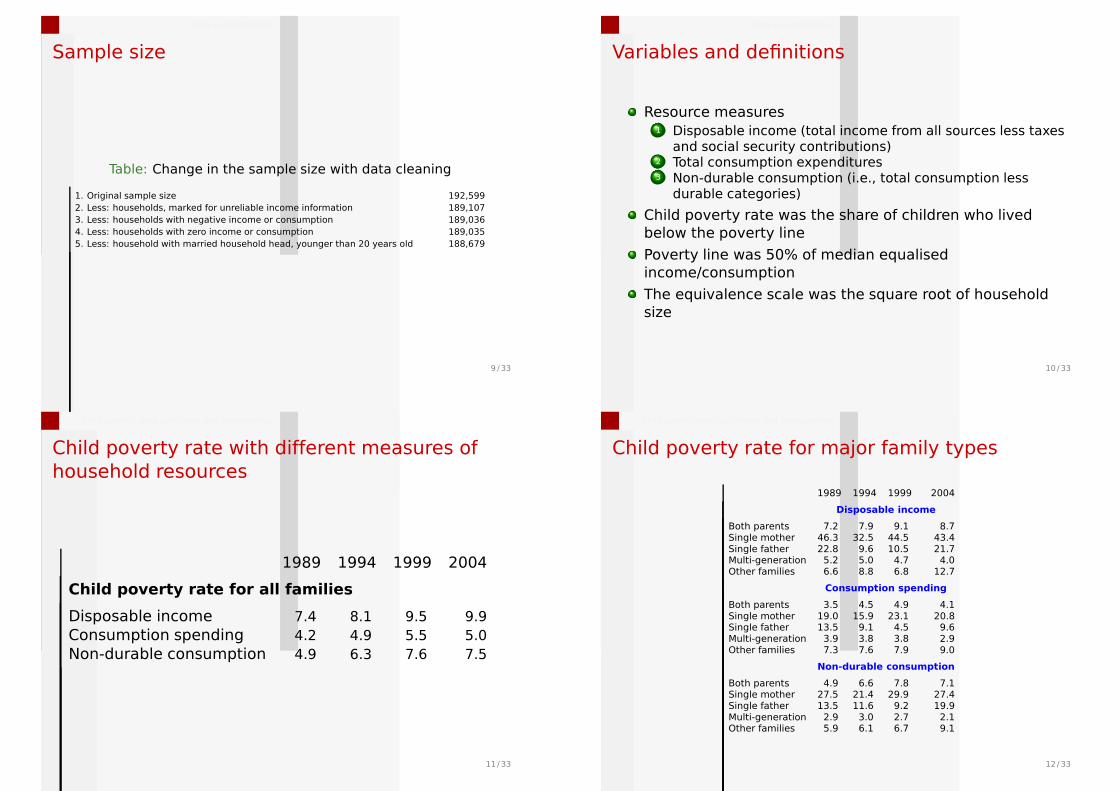
Child poverty rate with different measures of

household resources

1989 1994 1999 2004

Child poverty rate for all families

Disposable income 7.4 8.1 9.5 9.9

Consumption spending 4.2 4.9 5.5 5.0

Non-durable consumption 4.9 6.3 7.6 7.5

11 /33


Child poverty rate for major family types

1989 1994 1999 2004

Disposable income

Both parents 7.2 7.9 9.1 8.7Single mother 46.3 32.5 44.5 43.4Single father 22.8 9.6 10.5 21.7Multi-generation 5.2 5.0 4.7 4.0Other families 6.6 8.8 6.8 12.7

Consumption spending


Non-durable consumption


12 /33

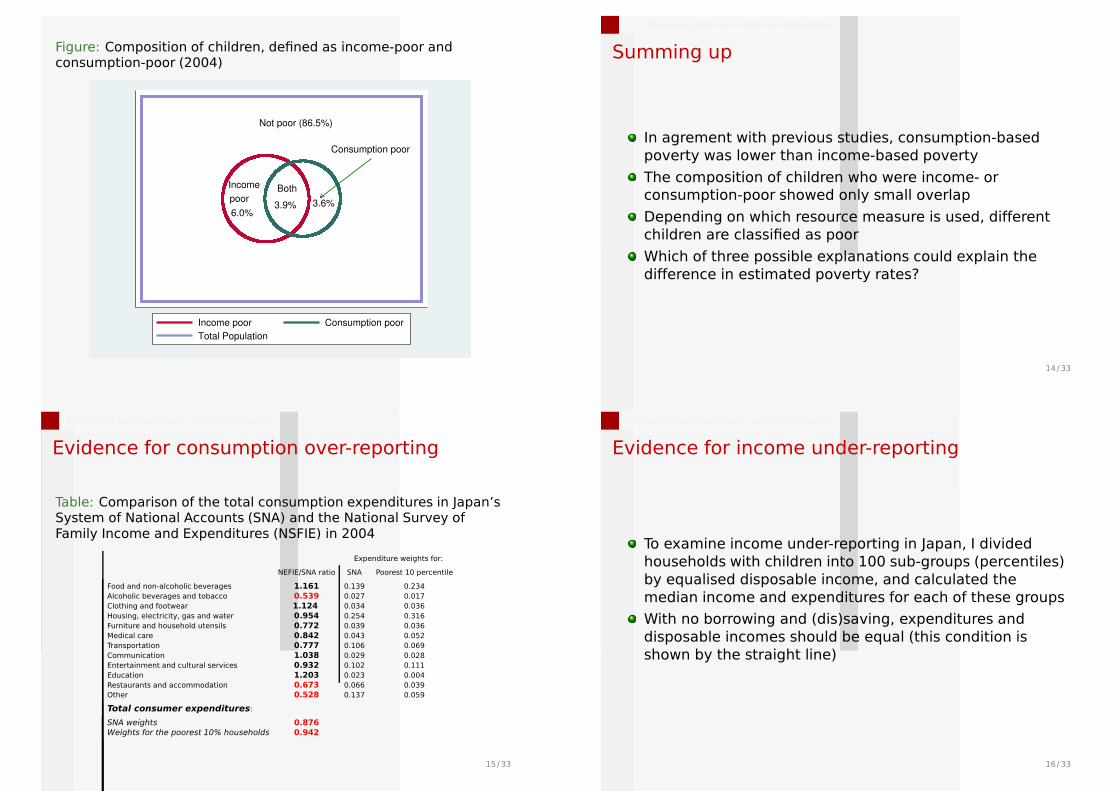
Figure: Composition of children, defined as income-poor andconsumption-poor (2004)

Income

6.0%

Consumption poor

3.6%3.9%

Not poor (86.5%)

poorBoth

Income poor Consumption poor

Total Population


Summing up

In agrement with previous studies, consumption-based

poverty was lower than income-based poverty

The composition of children who were income- or

consumption-poor showed only small overlap

Depending on which resource measure is used, different

children are classified as poor

Which of three possible explanations could explain the

difference in estimated poverty rates?

14 /33

Why poverty by consumption < poverty by income?

Evidence for consumption over-reporting

Table: Comparison of the total consumption expenditures in Japan’sSystem of National Accounts (SNA) and the National Survey ofFamily Income and Expenditures (NSFIE) in 2004

Expenditure weights for:

NEFIE/SNA ratio SNA Poorest 10 percentile

Food and non-alcoholic beverages 1.161 0.139 0.234

Alcoholic beverages and tobacco 0.539 0.027 0.017

Clothing and footwear 1.124 0.034 0.036

Housing, electricity, gas and water 0.954 0.254 0.316

Furniture and household utensils 0.772 0.039 0.036

Medical care 0.842 0.043 0.052

Transportation 0.777 0.106 0.069

Communication 1.038 0.029 0.028

Entertainment and cultural services 0.932 0.102 0.111

Education 1.203 0.023 0.004

Restaurants and accommodation 0.673 0.066 0.039

Other 0.528 0.137 0.059

Total consumer expenditures:

SNA weights 0.876

Weights for the poorest 10% households 0.942

15 /33


Evidence for income under-reporting

To examine income under-reporting in Japan, I divided

households with children into 100 sub-groups (percentiles)

by equalised disposable income, and calculated the

median income and expenditures for each of these groups

With no borrowing and (dis)saving, expenditures and

disposable incomes should be equal (this condition is

shown by the straight line)

16 /33

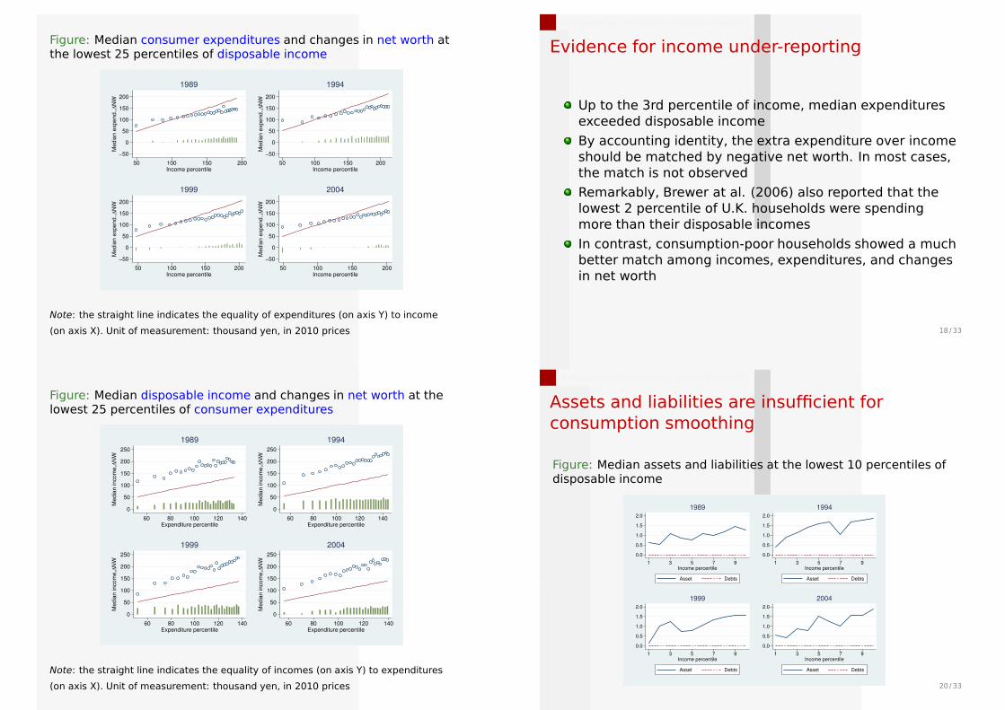
Figure: Median consumer expenditures and changes in net worth atthe lowest 25 percentiles of disposable income

−50

0

50

100

150

200

Media

n e

xpend.,

∆N

W

50 100 150 200Income percentile

1989

−50

0

50

100

150

200

Media

n e

xpend.,

∆N

W


1994

−50

0

50

100

150

200

Media

n e

xpend.,

∆N

W


1999

−50

0

50

100

150

200

Media

n e

xpend.,

∆N

W


2004

Note: the straight line indicates the equality of expenditures (on axis Y) to income

(on axis X). Unit of measurement: thousand yen, in 2010 prices


Evidence for income under-reporting

Up to the 3rd percentile of income, median expenditures

exceeded disposable income

By accounting identity, the extra expenditure over income

should be matched by negative net worth. In most cases,

the match is not observed

Remarkably, Brewer at al. (2006) also reported that the

lowest 2 percentile of U.K. households were spending

more than their disposable incomes

In contrast, consumption-poor households showed a much

better match among incomes, expenditures, and changes

in net worth

18 /33

Figure: Median disposable income and changes in net worth at thelowest 25 percentiles of consumer expenditures

0

50

100

150

200

250

Media

n incom

e,∆

NW

60 80 100 120 140Expenditure percentile

1989

0

50

100

150

200

250

Media

n incom

e,∆

NW


1994

0

50

100

150

200

250

Media

n incom

e,∆

NW


1999

0

50

100

150

200

250

Media

n incom

e,∆

NW


2004

Note: the straight line indicates the equality of incomes (on axis Y) to expenditures

(on axis X). Unit of measurement: thousand yen, in 2010 prices


Assets and liabilities are insufficient for

consumption smoothing

Figure: Median assets and liabilities at the lowest 10 percentiles ofdisposable income

0.0

0.5

1.0

1.5

2.0

1 3 5 7 9Income percentile

Asset Debts

1989

0.0

0.5

1.0

1.5

2.0


Asset Debts

1994

0.0

0.5

1.0

1.5

2.0


Asset Debts

1999

0.0

0.5

1.0

1.5

2.0


Asset Debts

2004

20 /33


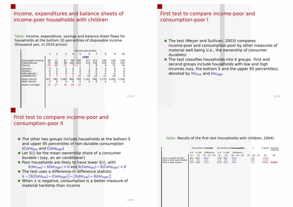
Income, expenditures and balance sheets of

income-poor households with children

Table: Income, expenditure, savings and balance sheet flows forhouseholds at the bottom 10 percentiles of disposable income(thousand yen, in 2010 prices)

Income percentiles

1 2 3 4 5 6 7 8 9 10

1989

Disposable income 49 73 87 99 108 117 123 128 134 139Expenditures 75 99 98 106 110 114 116 119 122 125Saving -29 -26 -11 -7 -1 3 8 9 11 14

d(Asset)+ 0 4 0 0 6 7 8 9 8 3d(Debt)+ 0 0 0 0 0 0 0 0 0 0d(RealAsset) = 0 0 0 0 0 0 0 0 0 0d(NetWorth) 0 7 1 1 10 10 13 11 14 8

Asset (stock) 617 545 1,069 858 769 1,101 992 1,170 1,456 1,254Debt (stock) 0 0 0 0 0 0 0 0 0 0

Asset coverage 14 27 42 44 37

21 /33

Tests for an accurate poverty measure

First test to compare income-poor and

consumption-poor I

The test (Meyer and Sullivan, 2003) compares

income-poor and consumption-poor by other measures of

material well-being (i.e., the ownership of consumer

durables)

The test classifies households into 4 groups. First and

second groups include households with low and high

incomes (say, the bottom 5 and the upper 95 percentiles),

denoted by Inclow and Inchigh

22 /33


First test to compare income-poor and

consumption-poor II

The other two groups include households at the bottom 5

and upper 95 percentiles of non-durable consumption

(Conslow and Conshigh)

Let S(i) be the mean ownership share of a consumer

durable i (say, an air conditioner)

Poor households are likely to have lower S(i), withS(Inclow)− S(Inchigh) < 0 and S(Conslow)− S(Conshigh) < 0

The test uses a difference-in-difference statistic

λ =�

S(Conslow)− Conshigh)�

−

�

S(Inclow)− S(Inchigh)�

When λ is negative, consumption is a better measure of

material hardship than income

23 /33

Table: Results of the first test (households with children, 2004)

Percentiles of income Percentiles of consumption λ p-value Favoredmeasure

0–5 5–100 Difference 0–5 5–100 Difference

(1) (2) (3) = (1)− (2) (4) (5) (6) = (4)− (5) (7) = (6)− (3) (8) (9)

Have a system kitchen 18.2 58.5 -40.3 14.8 58.7 -44.0 -3.6 0.054Have a solar water heater 3.1 7.6 -4.5 2.2 7.6 -5.4 -0.9 0.271Have a water heater 27.9 54.8 -27.0 21.0 55.2 -34.2 -7.2 <0.001 Cons.

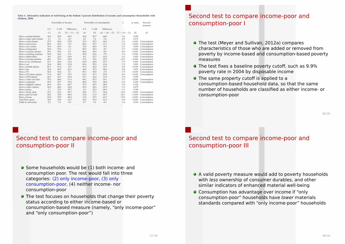
Table 6. Alternative indicators of well-being at the bottom 5 percent distribution of income and consumption (households withchildren, 2004).

Percentiles of income Percentiles of consumption λ p-value Favored

measure

0–5 5–100 Difference 0–5 5–100 Difference

(1) (2) (3) = (1)− (2) (4) (5) (6) = (4)− (5) (7) = (6)− (3) (8) (9)

Have a system kitchen 18.2 58.5 -40.3 14.8 58.7 -44.0 -3.6 0.054Have a solar water heater 3.1 7.6 -4.5 2.2 7.6 -5.4 -0.9 0.271Have a water heater 27.9 54.8 -27.0 21.0 55.2 -34.2 -7.2 <0.001 ConsumptionHave a microwave 89.5 93.4 -3.9 82.6 93.7 -11.1 -7.2 <0.001 ConsumptionHave a rice cooker 78.3 82.5 -4.2 72.9 82.8 -9.9 -5.7 0.005 ConsumptionHave a refrigerator 92.8 93.9 -1.1 85.5 94.3 -8.7 -7.7 <0.001 ConsumptionHave a vacuum cleaner 94.1 94.2 -0.1 86.6 94.6 -8.0 -8.0 <0.001 ConsumptionHave a washing machine 94.0 94.2 -0.2 86.8 94.6 -7.8 -7.6 <0.001 ConsumptionHave a dishwasher 8.6 23.5 -14.9 4.5 23.7 -19.2 -4.3 0.001 ConsumptionHave a sewing machine 48.1 72.0 -23.9 37.2 72.6 -35.5 -11.5 <0.001 ConsumptionHave an air conditioner 72.1 84.4 -12.2 65.0 84.8 -19.7 -7.5 0.001 ConsumptionHave a car 76.4 88.8 -12.4 69.6 89.2 -19.6 -7.2 0.001 ConsumptionHave a mobile phone 87.1 91.6 -4.5 79.3 92.0 -12.7 -8.2 <0.001 ConsumptionHave a fax 35.4 56.9 -21.6 30.6 57.2 -26.6 -5.0 0.031 ConsumptionHave a TV 92.6 92.4 0.1 85.1 92.8 -7.8 -7.9 <0.001 ConsumptionHave a CD stereo player 71.4 86.7 -15.3 63.3 87.1 -23.8 -8.5 <0.001 ConsumptionHave a DVD player 22.7 32.7 -10.0 19.1 32.9 -13.9 -3.9 0.055Have a video recorder 75.5 86.8 -11.3 68.1 87.2 -19.1 -7.7 <0.001 ConsumptionHave a computer 45.5 78.7 -33.2 40.8 79.0 -38.2 -5.0 0.030 ConsumptionHave a (digital) camera 60.6 85.3 -24.7 57.5 85.5 -28.0 -3.2 0.136Have a video camera 44.2 68.6 -24.4 43.3 68.6 -25.4 -1.0 0.679Have a piano 7.1 32.9 -25.7 6.0 32.9 -26.9 -1.2 0.349Have a study desk 55.7 76.4 -20.7 42.8 77.1 -34.4 -13.6 <0.001 ConsumptionHave a plot of land 24.2 70.8 -46.5 10.8 71.5 -60.7 -14.1 <0.001 ConsumptionHave a house 24.8 74.0 -49.2 12.0 74.7 -62.7 -13.5 <0.001 ConsumptionTotal floor space 36.9 53.6 -16.7 32.4 53.9 -21.5 -4.8 <0.001 ConsumptionChild in university 2.2 7.6 -5.3 0.7 7.6 -6.9 -1.6 0.016 Consumption

Note: the table compares income- and consumption-poor households with children at the bottom 5 percent of household distribution. For income and consumption, I used


Second test to compare income-poor and

consumption-poor I

The test (Meyer and Sullivan, 2012a) compares

characteristics of those who are added or removed from

poverty by income-based and consumption-based poverty

measures

The test fixes a baseline poverty cutoff, such as 9.9%

poverty rate in 2004 by disposable income

The same property cutoff is applied to a

consumption-based household data, so that the same

number of households are classified as either income- or

consumption-poor

26 /33



consumption-poor II

Some households would be (1) both income- and

consumption poor. The rest would fall into three

categories: (2) only income-poor, (3) only

consumption-poor, (4) neither income- nor

consumption-poor

The test focuses on households that change their poverty

status according to either income-based or

consumption-based measure (namely, “only income-poor”

and “only consumption-poor”)

27 /33



consumption-poor III

A valid poverty measure would add to poverty households

with less ownership of consumer durables, and other

similar indicators of enhanced material well-being

Consumption has advantage over income if “only

consumption-poor” households have lower materials

standards compared with “only income-poor” households

28 /33

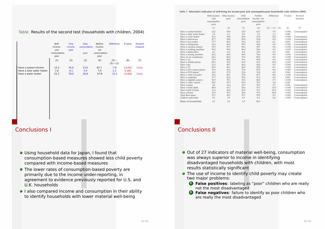
Table: Results of the second test (households with children, 2004)

Both

income-

and

consumption-

poor

Only

income-

poor

Only

consumption-

poor

Neither

income-

nor

consumption-

poor

Difference P-value Favored

measure

(1) (2) (3) (4) (5) =

(3)− (2)

(6) (7)

Have a system kitchen 12.2 30.9 23.0 62.7 -7.8 <0.001 Cons.

Have a solar water heater 1.8 6.1 4.9 7.9 -1.1 0.280

Have a water heater 21.2 39.0 26.8 57.8 -12.2 <0.001 Cons.

Table 7. Alternative indicators of well-being for income-poor and consumption-poor households with children (2004).

Both income-

and

consumption-

poor

Only income-

poor

Only

consumption-

poor

Neither

income- nor

consumption-

poor

Difference P-value Favored

measure

(1) (2) (3) (4) (5) = (3)− (2) (6) (7)

Have a system kitchen 12.2 30.9 23.0 62.7 -7.8 <0.001 ConsumptionHave a solar water heater 1.8 6.1 4.9 7.9 -1.1 0.280Have a water heater 21.2 39.0 26.8 57.8 -12.2 <0.001 ConsumptionHave a microwave 87.7 94.8 85.4 93.8 -9.4 <0.001 ConsumptionHave a rice cooker 77.7 80.5 74.4 83.2 -6.1 0.002 ConsumptionHave a refrigerator 91.6 94.5 85.5 94.4 -9.0 <0.001 ConsumptionHave a vacuum cleaner 92.9 95.7 86.2 94.7 -9.6 <0.001 ConsumptionHave a washing machine 93.0 95.6 86.4 94.6 -9.2 <0.001 ConsumptionHave a dishwasher 4.2 13.1 8.4 25.3 -4.7 0.001 ConsumptionHave a sewing machine 42.2 60.0 50.0 74.4 -9.9 <0.001 ConsumptionHave an air conditioner 69.2 80.4 70.9 85.6 -9.6 <0.001 ConsumptionHave a car 72.9 85.6 79.1 89.8 -6.5 <0.001 ConsumptionHave a mobile phone 85.3 92.2 81.8 92.2 -10.4 <0.001 ConsumptionHave a fax 31.0 49.7 40.4 58.6 -9.3 <0.001 ConsumptionHave a TV 90.9 94.1 86.0 92.8 -8.1 <0.001 ConsumptionHave a CD a stereo player 70.0 81.6 73.4 87.8 -8.2 <0.001 ConsumptionHave a DVD player 18.9 27.9 23.4 33.8 -4.5 0.026 ConsumptionHave a video recorder 73.0 84.7 75.8 87.7 -8.8 <0.001 ConsumptionHave a computer 37.7 62.6 55.6 81.5 -6.9 0.002 ConsumptionHave a (digital) camera 56.5 78.1 70.6 86.8 -7.5 <0.001 ConsumptionHave a video camera 42.9 57.2 55.4 70.1 -1.8 0.443Have a piano 4.8 16.4 12.7 35.2 -3.7 0.024 ConsumptionHave a study desk 48.8 63.7 50.4 79.1 -13.3 <0.001 ConsumptionHave a plot of land 11.4 43.0 22.0 76.1 -21.0 <0.001 ConsumptionHave a house 12.5 45.7 24.9 79.3 -20.8 <0.001 ConsumptionTotal floor space 31.7 42.7 37.7 55.5 -5.0 <0.001 ConsumptionChild in university 0.5 3.8 0.9 8.3 -2.8 <0.001 Consumption

Share of households 4.7 5.5 5.5 84.3

Note: the table compares characteristics of households that are added to poverty by income- and consumption-based poverty measures. For income and consumption, I used disposable

Conclusion

Conclusions I

Using household data for Japan, I found that

consumption-based measures showed less child poverty

compared with income-based measures

The lower rates of consumption-based poverty are

primarily due to the income under-reporting, in

agreement to evidence previously reported for U.S. and

U.K. households

I also compared income and consumption in their ability

to identify households with lower material well-being

31 /33

Conclusion

Conclusions II

Out of 27 indicators of material well-being, consumption

was always superior to income in identifying

disadvantaged households with children, with most

results statistically significant

The use of income to identify child poverty may createtwo major problems:

1 False positives: labeling as “poor” children who are reallynot the most disadvantaged

2 False negatives: failure to identify as poor children whoare really the most disadvantaged

32 /33

Conclusion

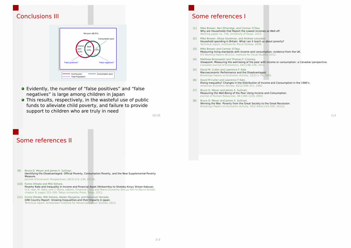
Conclusions III

Income

6.0%

Consumption poor

3.6%3.9%

Not poor (86.5%)

poorBoth

False positives? False negatives?

Income poor Consumption poor

Total Population

Evidently, the number of “false positives” and “false

negatives” is large among children in Japan

This results, respectively, in the wasteful use of public

funds to alleviate child poverty, and failure to provide

support to children who are truly in need33 /33

Some references I

[1] Mike Brewer, Ben Etheridge, and Cormac O’Dea.Why are Households that Report the Lowest Incomes so Well-off.Working paper no. 736, University of Essex, 2013.

[2] Mike Brewer, Alissa Goodman, and Andrew Leicester.Household spending in Britain: What can it teach us about poverty?Technical report, Institute for Fiscal Studies, 2006.

[3] Mike Brewer and Cormac O’Dea.Measuring living standards with income and consumption: evidence from the UK.IFS Working Papers W12/12, Institute for Fiscal Studies, 2012.

[4] Matthew Brzozowski and Thomas F. Crossley.Viewpoint: Measuring the well-being of the poor with income or consumption: a Canadian perspective.Canadian Journal of Economics, 44(1):88–106, 2011.

[5] David M. Cutler and Lawrence F. Katz.Macroeconomic Performance and the Disadvantaged.Brookings Papers on Economic Activity, 22(2):1–74, 1991.

[6] David M Cutler and Lawrence F Katz.Rising Inequality? Changes in the Distribution of Income and Consumption in the 1980’s.American Economic Review, 82(2):546–551, 1992.

[7] Bruce D. Meyer and James X. Sullivan.Measuring the Well-Being of the Poor Using Income and Consumption.Journal of Human Resources, 38:1180–1220, 2003.

[8] Bruce D. Meyer and James X. Sullivan.Winning the War: Poverty from the Great Society to the Great Recession.Brookings Papers on Economic Activity, 45(2 (Fall)):133–200, 2012a.

1 / 2

Some references II

[9] Bruce D. Meyer and James X. Sullivan.Identifying the Disadvantaged: Official Poverty, Consumption Poverty, and the New Supplemental PovertyMeasure.Journal of Economic Perspectives, 26(3):111–136, 2012b.

[10] Fumio Ohtake and Miki Kohara.Poverty Rate and Inequality in Income and Financial Asset (Hinkonritsu to Shotoku Kinyu Shisan Kakusa).In K. Iwai, M. Seko, and Y. Okina, editors, Financial Crisis and Macro Economy (Kin-yu Kiki to Macro Keizai),chapter 8, pages 253–285. Tokyo University Press, Tokyo, 2011.

[11] Fumio Ohtake, Miki Kohara, Naoko Okuyama, and Katsunori Yamada.GINI Country Report: Growing Inequalities and their Impacts in Japan.Technical report, Amsterdam Institute for Advanced Labour Studies, 2013.

2 / 2

Child poverty in Japan: comparing the accuracy of … poverty by consumption < poverty by income?...

Documents

Transcript of Child poverty in Japan: comparing the accuracy of … poverty by consumption < poverty by income?...