An ESRC Research Group

Subjective well-being poverty versus income poverty and capabilities poverty?

GPRG-WPS-003

Geeta Gandhi Kingdon and John Knight

Global Poverty Research Group

Website: http://www.gprg.org/

The support of the Economic and Social Research Council (ESRC) is gratefully acknowledged. The work was part of the programme of the ESRC Global Poverty Research Group.

1

Subjective well-being poverty versus income poverty and capabilities poverty?

GPRG-WPS-003

by

Geeta Gandhi Kingdon and John Knight

Global Poverty Research Group Centre for the Study of African Economies

Department of Economics University of Oxford

December 2004

Correspondence: Geeta G. Kingdon, Department of Economics, University of Oxford, Oxford OX1 3UQ, United Kingdom; tel: 00 44 1865 271065; email: geeta.kingdon@economics.ox.ac.uk Acknowledgements: We would like to thank John Helliwell for stimulating discussions about the ideas in this paper. In addition to workshop participants at the GPRG workshop, Oxford, and seminar participants at the Wellbeing in Developing Countries (WeD) Research Group at Bath University, we would like to thank Alan Krueger, Allister McGregor, Wendi Olsen, John Toye and an anonymous referee for helpful comments on the paper. Any errors are ours. The support of the Economic and Social Research Council (ESRC) is gratefully acknowledged. The work was part of the programme of the ESRC Global Poverty Research Group.

2

Well-being poverty versus income poverty and capabilities poverty?

Abstract

The conventional approach of economists to the measurement of poverty in poor countries is to use measures of income or consumption. This has been challenged by those who favour broader criteria for poverty and its avoidance. These include the fulfilment of ‘basic needs’, the ‘capabilities’ to be and to do things of intrinsic worth, and safety from insecurity and vulnerability. This paper asks: to what extent are these different concepts measurable, to what extent are they competing and to what extent complementary, and is it possible for them to be accommodated within an encompassing framework? There are two remarkable gaps in the rapidly growing literature on subjective well-being. First, reflecting the availability of data, there is little research on poor countries. Second, within any country, there is little research on the relationship between well-being and the notion of poverty. This paper attempts to fill these gaps. Any attempt to define poverty involves a value judgement as to what constitutes a good quality of life or a bad one. We argue that an approach which examines the individual’s own perception of well-being is less imperfect, or more quantifiable, or both, as a guide to forming that value judgement than are the other potential approaches. We develop a methodology for using subjective well-being as the criterion for poverty, and illustrate its use by reference to a South African data set containing much socio-economic information on the individual, the household and the community, as well as information on reported subjective well-being. We conclude that it is possible to view subjective well-being as an encompassing concept, which permits us to quantify the relevance and importance of the other approaches and of their component variables. The estimated subjective well-being functions for South Africa contain some variables corresponding to the income approach, some to the basic needs (or physical functioning) approach, some to the relative (or social functioning) approach, and some to the security approach. Thus, our methodology effectively provides weights of the relative importance of these various components of subjective well-being poverty.

3

1. Introduction

Empirical research by economists on poverty in developing countries has generally been

concerned with its measurement in terms of income and consumption. Behind this metric lies

the concept of utility, or welfare, which people are assumed to derive from income and

consumption. Yet there has been little attempt to measure poverty in terms of reported utility,

i.e. subjectively perceived welfare. In this paper we shall explore the latter approach,

attempting to gain insights from new research on the economics of happiness for

understanding poverty in developing countries.

Economic research on reported happiness (or subjective well-being - we use the terms

interchangeably) is sparse and recent but growing rapidly. It is apparent from this literature

that there are two important gaps to be filled. First, reflecting the availability of data, there is

little research on subjective well-being on poor countries (Diener and Biswas-Diener, 2000)1.

Second, within any country, there is little research on the relationship between subjective

well-being and conventional measures of poverty. The purpose of this paper is to help bridge

these two gaps.

Some theoretical research on poverty in developing countries has eschewed income or

consumption as the evaluative criterion. Alternative criteria have been put forward, some in a

form which eschews utility as the evaluative criterion, e.g. the fulfilment of basic needs and

the extent of peoples’ capabilities to be and to do things of intrinsic worth. Such approaches

suggest a broader set of measures for assessing poverty than just income and consumption,

including public provision of non-marketed services, such as sanitation, health care and

education (inputs) or healthiness, life expectancy and literacy (outputs). While retaining utility

as our evaluative criterion, and using subjectively perceived well-being as our measure of

utility, we shall propose a method of incorporating not only income or consumption but also

other determinants of the quality of life (such as these) into the analysis of poverty.

In this paper we shall consider the relationship between what we shall call “subjective well-

being poverty” and poverty as it is otherwise measured in poor countries. The paper is

1 Ravallion and Lokshin (2001) and Graham and Pettinato (2002) are rare exceptions.

4

methodological in emphasis, setting out the issues, the appropriate methods and the data

requirements for a programme of research.

Section 2 will provide a review of the literature on happiness, explaining the solid results so

far and the hypotheses that they suggest for the study of poor people in poor countries.

Section 3 provides the methodology, explaining the estimation of subjective well-being

functions, their relationship to income functions, and their relationship to various other

concepts of poverty. The argument is illustrated in Section 4 with an available data set, the

SALDRU national household survey for South Africa, 1993. Section 5 draws conclusions

from the analysis.

2. Literature Survey

This section contains four parts. We start with relevant aspects of the literature on subjective

well-being, and then turn to relevant aspects of the literature on poverty. We examine the

research on the interface between these two topics and, finding little, we put the case for

exploring the subjective well-being approach to poverty.

There is a good survey of the literature on economic aspects of happiness – some of it

interdisciplinary and some by non-economists – by Frey and Stutzer (2002). Their evaluation

of this growing field is upbeat and their prognosis is promising. Layard (2003a), in surveying

the field, takes an even more sanguine view: “The scientific study of happiness is only just

beginning. It should become a central topic in social science”. Much of the research has

involved the estimation of happiness functions, in which happiness (subjectively rated on an

ordinal or cardinal scale) is the dependent variable and various socio-economic characteristics

of the individual, household or community are used as explanatory variables. Some of the

research relates to particular countries (generally advanced economies), using either cross-

section or panel data sets; and some covers many countries, normally using comparable data

sets derived from the World Values Survey.

The main findings from the general literature are the following. First, happiness increases

with absolute income, ceteris paribus, but not proportionately and at a diminishing rate (Frey

and Stutzer, 2002). Moreover, differences in income explain only a small proportion of the

variation in happiness among people. The importance of income appears to vary among

5

countries: happiness levels are lowest in the poorest countries but the relationship between

income and happiness is weak beyond a fairly low international level of income per capita.

This is consistent with the argument that happiness depends in part on the gratification of

certain absolute biological and psychological needs (Veenhoven, 1991).

The limited role of absolute income is further suggested by the fact that income and happiness

are positively related in cross-section but not in time-series studies. For instance, in the United

States and in Japan, real income per capita increased over time but the mean happiness score

remained constant. It is possible that mean happiness did not rise over time because aspiration

levels adjusted to, and so rose along with, mean incomes in the society, and happiness varied

positively with income but negatively with aspirations (Easterlin, 2001). The second main

finding, therefore, is that happiness depends on relative income, defined by the reference

group or the reference time that people have in mind.

This finding is consistent with the long-established literature on relative deprivation

(Duesenberry, 1949; Runciman, 1966). Perceptions of subjective well-being depend on the

context: people compare themselves with others in society or with themselves in the past, and

they feel deprived if they are doing less well than the comparator. This raises the questions:

what comparisons do people make; how wide are the orbits of comparison? Duesenberry

(1949) stressed previous income or consumption, and better-off people, as the frames of

reference. Runciman (1966) suggested informational and social reasons why the frame of

reference can be narrow. Perceptions of relative deprivation are expected to reduce happiness.

It is also possible that perceptions of relative advantage will raise happiness. Thus, a person’s

position in the income distribution of the relevant reference group may govern happiness.

Happiness might be responsive to income ranking over the range (say, below the median) in

which people feel relatively deprived, or it might increase monotonically throughout the

income distribution.

Absolute and relative incomes are not the only economic determinants of happiness. Being

unemployed is found to reduce happiness independently of its effect on income (Clark and

Oswald, 1994; Winkelmann and Winkelmann,1998). The general unemployment rate also has

a depressing effect, suggesting that having a higher risk of becoming unemployed reduces

happiness. Another indication of economic insecurity is inflation: countries and periods with

higher inflation display lower happiness, ceteris paribus (Di Tella et al, 2001). Subjective

6

well-being is influenced by several factors that are non-economic or potentially so, such as

age, sex, marital status, health status, education, social capital, religion, and social and

political institutions (Helliwell, 2002).

We turn to the literature on poverty. Sen (1983) introduced the concept of a person’s

“capabilities” to be and to do things of intrinsic worth, i.e. resources adequate to achieve a

specified set of “functionings”. He argued that absolute deprivation in terms of a person’s

capabilities can imply relative deprivation in terms of income, resources or commodities, e.g.

for taking part in the life of the community, for the avoidance of shame, or for the

maintenance of self-respect. He favoured the capability to function as the criterion for

assessing the standard of living, and by implication poverty, rather than the utility that might

be derived from using that capability. Thus, Sen eschewed the “welfarist” approach to

poverty with its underlying assumption that the evaluative criterion is the utility that people

derive from goods and services. However, he neither offered a practical criterion for

evaluating the various capabilities to function nor sought any aggregation of the social values

of the separate capabilities.

Atkinson and Bourguignon (1999) use the same framework but from a welfarist perspective.

They regard poverty as “inadequate command over economic resources” but view this as an

intermediate concern, the ultimate concern being in terms of “capabilities” in the sense of

Sen. The absolute set of capabilities translates into a set of goods requirements which is

relative to a particular society and its standard of living. This leads them to formulate a

concept in line with the World Bank’s World Development Report (1990, p.26), that a

“…poverty line can be thought of as comprising two elements: the expenditure necessary to

buy a minimum level of nutrition and other basic necessities and a further amount that varies

from country to country, reflecting the cost of participating in the everyday life of the

society”. There is a hierarchy of capabilities. The first concerns physical functioning and

requires a set of goods fixed in absolute terms; this capability has priority. The second

capability concerns social functioning and requires a set of goods that depends on the mean

level of income. These authors see capabilities and functionings as contributing to welfare,

but they do not consider subjective well-being as the measure of welfare nor do they explicitly

adopt an encompassing approach.

7

Attempts have been made to compare and combine different measures of poverty. For

instance, Laderchi et al (2003) examine and contrast four different approaches to the

definition of poverty (not including the subjective well-being approach). They show

empirically that there is little overlap in individuals falling into the different types of poverty,

for instance (their definitions of) income poverty and capabilities poverty. They favour

aggregation of the various dimensions of poverty but conclude that “in general there is no

right way of aggregating” (p.246). Clark (2004) espouses the capabilities approach to poverty

but, on the basis of a South African case study of poor peoples’ perceptions of a good life,

reaches the qualitative conclusion that both income and utility are important components of

functioning.

Little has yet been written on the interface between subjective well-being and poverty.

Ravallion and colleagues have pioneered the use of subjective perceptions in the analysis of

poverty in developing countries. Pradhan and Ravallion (2000) use household surveys for

Jamaica and Nepal which ask whether total consumption (or consumption of food, or housing,

etc.) is adequate for household minimum needs. This enables them to estimate “subjective

poverty lines”. They compare these with objective poverty lines and note interesting

differences, e.g. a greater subjective than objective urban-rural difference in poverty, and

greater perceived than actual household scale economies in consumption.

Ravallion and Lokshin (2001, 2002) use a household panel data set for Russia which asked

people to classify themselves on a nine-step ladder along a dimension from “poorest” to

“rich”. Households are ranked both according to their subjective poverty/wealth status and

according to their income (normalised by the relevant objective poverty line). The two

rankings are significantly positively correlated but the matching is nevertheless weak: many

who classify themselves as subjectively poor are not objectively so, and vice versa. The

reason for the discrepancy is explored by incorporating into the subjective ranking equation

such factors as education, employment status, health status and permanent income. The

subjective classification takes these factors into account as well as current income. Although

rank changes are treated as representing changes in utility (Ravallion and Lokshin, 2001), the

ranking is not necessarily an indication of subjective well-being. Rather, it appears to ask

people to gauge their relative position in the hierarchy of poverty and wealth, and is partly a

test of how well informed they are about this.

8

The underlying criticism of Sen (1983), Ravallion and Lokshin (2002), and Diener and

Biswas-Diener (2002) of happiness as a measure of poverty is that it represents a particular

mental reaction to the use of a capability rather than the capability itself (Sen), that it need not

be closely related to subjectively perceived poverty (Ravallion and Lokshin), that it is too

broad (Sen, Ravallion and Lokshin), and that it is a necessary but not a sufficient condition for

assessing quality of life (Diener and Biswas-Diener). In our view the most serious criticism is

the first of these. In the words of Sen (1984, pp.308-9): “The most blatant forms of

inequalities and exploitations survive in the world through making allies out of the deprived

and exploited. The underdog learns to bear the burden so well that he or she overlooks the

burden itself. Discontent is replaced by acceptance…suffering and anger by cheerful

endurance. As people learn to adjust …the horrors look less terrible in the metric of utilities”.

We intend nevertheless to explore the happiness approach, for the following reasons. First, we

place value on individual freedom, and thus on the individual’s clearly expressed views about

her own well-being, and we are loath to have these over-ruled by values emerging unclearly

from elsewhere. However, if another value judgement is sought, the objective of alleviating

subjectively felt misery and raising peoples’ sense of well-being is a commonly held value

judgement, which underlies much of the concern that is voiced about poverty in developing

countries. Second, the use of a multivariate analysis makes it possible to isolate the average

effects of selected particular determinants of happiness without having to worry about the

many unobservables that contribute to human happiness and which make some people

naturally happier than others (unless these are correlated with the observed determinants).

Third, provided that utility is accepted as the evaluative criterion, it is possible to treat

subjective well-being as an encompassing concept, which enables us to quantify the relevance

and importance of the other approaches to poverty and of their components. It will be

necessary, however, to consider how human ability to adapt and to take a rosy view of a bad

situation can affect our estimates of the relationship between subjective well-being and its

determinants.

3. Methodology and Hypotheses

Our objective is to discover whether and how happiness can be explained by economic and

non-economic variables, and what light this can throw on the concept of poverty. We

therefore begin with the subjective well-being function

9

ininii uXbaW ++= . (1)

where iW represents subjective well-being and nX is a vector of n socio-economic variables.

iW is normally available as a multiple choice variable (of the sort “are you 1. very happy; 2.

happy; 3. so-so; 4. unhappy; 5. very unhappy?”). The appropriate estimation procedure is

therefore by means of a polychotomous probit or logit equation. The selection of nX depends

on the research hypotheses but also on what variables the data set has to offer. In the absence

of a well-articulated model carrying theoretical predictions, our approach is exploratory and is

influenced by the criteria that have been proposed in the literature for defining and assessing

poverty.

The vector of estimated coefficients nb provides the weights that indicate the relative

importance of different contributors to subjective well-being. The potential value of this

exercise can be illustrated by the deficiencies of the UNDP’s Human Development Index.

This is calculated by according equal weights to its three components – income per capita,

educational attainment, and life expectancy (UNDP, 2000). The value judgement implicit in

this weighting need not correspond at all well to the valuations of these capabilities made by

individuals in society. Subjective well-being may be a narrow metric but at least it

corresponds to individual valuations and it is a metric that can be measured.

The estimated subjective well-being function can be harnessed to examine the relationships

between the subjective well-being criterion for poverty and other criteria. These include the

conventional income criterion and, within the capabilities approach, the physical functioning

criterion and the social functioning criterion. Consider first the relationship between

subjective well-being poverty and income poverty. An obvious question concerns the extent

of overlap between the two. This can be examined by dividing the sample into m quantiles

according to the values of W and then into m quantiles of corresponding sizes according to

income ranking. A second exercise is to include income ( yX ) among the explanatory

variables in the subjective well-being equation and to examine its importance in determining

10

W relative to other determinants (the importance of income is indicated by the coefficient yb

and the contribution of yX to explaining the variation in W )2.

Although they are conceptually distinct, there is potentially a good deal of overlap between

the capabilities and the subjective well-being approaches to poverty. Both capabilities and

subjective well-being are likely to be positive functions of income. The various other

characteristics that are normally hypothesised to give people the capability to function well

are also prime suspects for raising happiness. The subjective well-being function should thus

include variables ( eXX ,...1 ) that correspond to physical functioning. These might comprise

components of “basic needs” such as nutrition, clothing, shelter, sanitation, health and

literacy. The function should also include variables ( he XX ,...1+ ) that correspond to social

functioning. These might take the form of proxies for the capability to meet the norms of

society and to interact well with society. Relative concepts are likely to figure: the relevant

reference groups need to be investigated. The group might be defined in terms of income,

ethnicity, residence or even time. It is thus possible to attach weights to physical and to social

functioning, and to their components. It is also possible to measure the relative importance of

the variables hypothesised to denote capabilities in the determination of subjective well-being.

By introducing a time dimension and using panel data, the literature on poverty often

distinguishes between chronic and transient poverty. Underlying this distinction is the notion

that the ill-effects are best measured by aggregating the indicator of poverty over time.

Expectations do not necessarily enter the story. However, by introducing proxies for

insecurity into the subjective well-being function, the subjective well-being approach can be

used to incorporate expectations. It is possible to examine the effect of prospective future

poverty on current happiness.

Finally, it is appropriate to include certain variables which do not fit into any of the

approaches to poverty outlined above, some of which fall outside the normal purview of

economists or policy-makers. These might include such demographic, geographic and social

variables as age, gender, family composition, marital status, residential location, religion,

social network, trust, and social participation. In part they serve as control variables; in part

2 There are obvious issues of endogeneity and causality which will be discussed below.

11

they serve to emphasise that subjective well-being can depend on a broad range of factors,

many of which are non-economic.

The notion that both absolute and relative poverty measures are relevant has implications for

the use of happiness measures in poverty analysis. We expect inadequate physical functioning

(such as hunger, lack of shelter and lack of warmth) to cause unhappiness. It is also plausible

that inadequate social functioning (such as alienation, shame and lack of self-respect) causes

unhappiness. Insofar as inadequate functioning reduces happiness, ceteris paribus, the

relationship between income and functioning determines the relationship between income and

happiness. When an individual’s income rises from a low level, happiness rises as the extent

of both absolute and relative poverty is reduced; when physical functioning is achieved, a

further rise in income can still raise happiness if social functioning is improved. Ceteris

paribus, a negative relationship between inadequacy of functioning and happiness might

therefore produce diminishing gains in individual happiness as income rises beyond first the

absolute and then the relative poverty level.

The coefficients estimated in the subjective well-being function isolate the average effects of

each explanatory variable for the sample as a whole, whereas we are interested primarily in

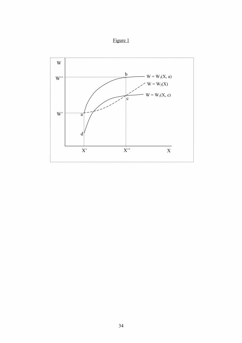
the poor. Consider the relationship between subjective well-being (W) and the vector of

“resources” (X) that produce subjective well-being. For simplicity, assume that resources can

be aggregated and measured cardinally (X). Figure 1 illustrates. If the poor (those with low X)

are subject to the same “happiness production function” as the non-poor (the continuous curve

)(1 XWW = ), we might expect the function to exhibit diminishing returns to resources, i.e. to

be concave (to the X axis). Apart from their corresponding to the normal assumption of

diminishing marginal utility, diminishing returns might reflect the fulfilment first of physical

functionings (basic needs) and then of social functionings (position in society). By contrast,

we have noted Sen’s argument (Sen, 1984) that the poor manage to adjust to hardship, i.e. of

necessity they become more efficient “pleasure machines”, so increasing their happiness

relative to their resources. In that case the subjective well-being function can be linear instead

of concave, or even convex (the continuous curve )(2 XWW = ).

It is possible that both functions are relevant: the effect of additional resources on the

subjective well-being of the poor might depend on whether there is an accompanying change

12

in attitudes or aspirations. The current poor (at point a, corresponding to (X’, W’)) may

experience the steeper, continuous curve, ),(1 aXWW = in the short run, given an expectation

of remaining poor. Thus they move to point b if their resources increase to X’’. Gradually

over time, however, they adjust to the higher level of resources, so moving to point c. Thus

the long run subjective well-being function is depicted by the flatter, dashed curve

)(2 XWW = , reflecting full adjustment to each level of resources. Similarly, a fall in

resources from point c corresponding to (X’’, W’’) involves a short term move along

),(1 cXWW = to point d at X’. Given time to adjust to their new situation, however, the newly

poor become reconciled to their lot, their aspirations are lowered and point a is restored. We

need to discover whether and how the poor and the non-poor differ in the way that their

happiness responds to additional resources.

The subjective well-being concept of poverty might be treated as competing with income,

capabilities and other concepts of poverty. We prefer to view it as an encompassing concept,

which permits us to quantify the relevance and importance of the other approaches and of

their components. Ultimately, the concept of poverty requires a value judgement as to what

constitutes a good life or a bad one. Our starting point is that an approach that examines the

individual’s own perception of well-being is less imperfect, or more quantifiable, or both, as a

guide to forming that value judgement than are the other possible approaches.

4. An Illustration from South Africa

The SALDRU national household survey of 1993 in South Africa was carried out by the

South African Labour and Development Research Unit (SALDRU) of the University of Cape

Town. The dataset contains information on about 8,800 households and is patterned on the

World Bank’s Living Standards Measurement Studies, with modules on household

demographics, employment, health, income and expenditure, etc. as well as community

information. Section 9 of this survey is on perceived quality of life and it contains, inter alia,

the question: “Taking everything into account, how satisfied is this household with the way it

lives these days?” The five options available in the pre-coded response were ‘very satisfied’,

‘satisfied’, ‘neither satisfied nor dissatisfied’, ‘dissatisfied’, and ‘very dissatisfied’.

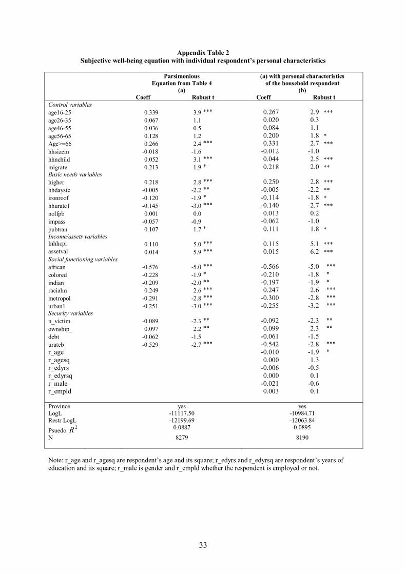
While the individual respondent to the survey answered the question, the question itself

related to the satisfaction of the household as a whole rather than to that individual’s personal

13

subjective well-being only. This raises the possibility that the individual was giving the

answer mostly with his own personal satisfaction level in mind rather than that of the

household as a whole. In order to address this concern, we check the robustness of the

findings to inclusion of the individual respondent’s own personal characteristics in the

analysis. Appendix Table 2 shows that, controlling for household characteristics, individual

characteristics are generally unimportant in our subjective well-being equations. This is not

surprising if, as is likely, there are interdependencies in perceived well-being among members

of the household.

The discussion comes in two parts. First, we ask to what extent our measure of subjective

well-being corresponds with the income measure that is most commonly used as a proxy for

well-being. We also examine whether the determinants of these two measures affect them in

the same direction and with similar intensity. Second, we examine the impact on subjective

well-being of factors that meet basic needs (physical functioning), social needs (social

functioning), and security needs of households.

4.1 Subjective well-being poverty versus income poverty?

The survey yields data on about 8,300 households after removing observations with missing

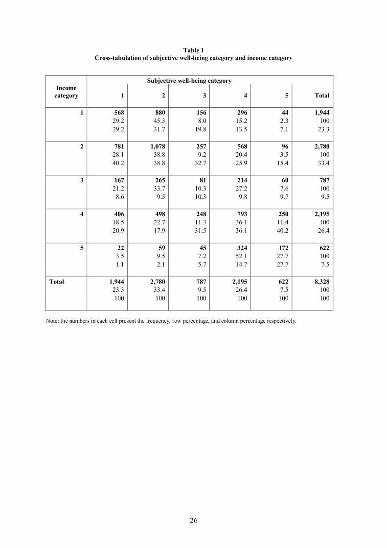
values for key variables. Table 1 presents a cross-tabulation of subjective well-being category

and income category. The former takes five values, from ‘very dissatisfied’ (coded as 1) to

‘very satisfied’ (coded as 5). The distribution of households across happiness categories is

uneven: 23% of all households reported being ‘very dissatisfied’; 33% as being ‘dissatisfied’;

only 10% as ‘neither satisfied nor dissatisfied’; 26% as ‘satisfied’ and a mere 8% as being

‘very satisfied’. Instead of using household per capita income quintiles, therefore, we have

divided the data into income categories as follows: the poorest 23% of the households (in

terms of per capita income) are in income category 1 (to correspond with the 23% of

households in the lowest subjective well-being category); the next 33% of households - in the

ordering of households by per capita income - are in income category 2, to correspond with

the 33% that are in the second happiness category, and so on.

The table shows that there is a poor degree of coincidence between these two measures.

Only in the second and fourth cells on the leading diagonal is the cell percentage frequency

highest among all cells in that row. For instance, of all the households in the poorest income

14

category, only 29% are in the lowest happiness category, although 75% are in the lowest two

happiness categories. Similarly, of those in the richest income category, only 28% are in the

highest happiness category. The best fit comes when we consider the two lowest categories

together: 70% of households defined as income-poor in this way were also subjective well-

being poor (and, by construction, vice versa). The overall correlation coefficient between

income category and subjective well-being category is +0.358. Thus, while income is

positively correlated with happiness, it is an imperfect predictor of happiness.

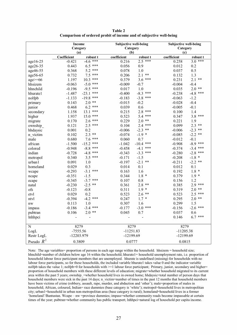
Table 2 examines whether various factors affect income and happiness in the same way.

Since our subjective well-being variable, and thus by design our income variable, is discrete

and takes values from 1 to 5 that are inherently ordered, the ordered probit is used to model

both income category and happiness category3. The pseudo R-square in an ordered probit can

be expected to take a low value. However, it has a higher value in the income than in the

happiness equation. All variables are defined in the notes to the table. The gender and

education level of individual members of the household are averaged across all household

members aged 16 and above. Thus the variable male represents the proportion of male

members and the education dummy variables primary, junior, secondary and higher represent

the proportion of household members with these levels of education. The age variables

represent the proportion of adult household members (16 years and older) within the specified

age ranges. Persons aged 0-15 are included by way of the variable ‘number of children in the

household’ (hhnchild). Other variables are household-level variables or community-level

variables.

In Table 2, household per capita income category is significantly determined by productive

characteristics such as age and education, but also by the household unemployment rate

(hhurate), race (African, Coloured, Indian), and location (urban, metropol, province), etc.

Several variables have quite different, or even opposing, effects on income and life-

satisfaction levels. For instance, comparing columns (a) and (b), youth (age16-25) is

associated with low income but high subjective well-being. Living in a metropolitan city

(metropol) raises income but lowers happiness. Poor health, as measured by number of days

household members have been sick in the past 14 days (hhdaysic), has no significant impact

on income but lowers perceived well-being significantly. The percentage of male members in

3 In Table 2 (and throughout the paper) standard errors have been corrected for clustering.

15

the household (male) significantly raises income but has no impact on happiness. Six of the

eight coefficients on the province dummy variables have opposing signs in the income and

happiness equations. Thus, not all factors or conditions that raise income also raise

happiness, and some even lower happiness.

Even when the signs are the same, the extent of association of several variables with income

differs substantially from that with happiness. For instance, while being African depresses

both income and happiness, the negative coefficient on African is very significantly greater in

the income equation than in the happiness equation. Similarly the association of age with

income rank is much greater than its association with happiness rank. The same remarks

apply to the coefficients on household size (hhsize), number of children aged 15 or below

(hhnchild), household unemployment rate (hhurate) and the education variables (primary,

junior, secondary, higher). We cannot assume that if a characteristic is good for generating

income, it is commensurately good, or even good at all, for generating happiness.

Several of the variables included in the subjective well-being equation in column (b) have a

direct impact on perceived well-being and also an indirect impact via their effect on

household income. Column (c) adds the natural log of household per capita income (lnhhpci)

to the happiness equation. Happiness increases powerfully with income, but the inclusion of

income does not affect the coefficients of other variables. The marginal effect of lnhhpci on

the probability of being in subjective well-being poverty (i.e. being in the lowest two life-

satisfaction categories) is 0.0572. Given a standard deviation of 1.4121, an increase in

lnhhpci from one standard deviation below to one standard deviation above the mean would

reduce the risk of subjective well-being poverty by 16.2 percentage points, which is not a

particularly large effect, given that 55% of all households are in the bottom two satisfaction

categories. When income is not constrained to enter linearly, there appear to be increasing

returns to income: if lnhhpci and its square are included, only the squared term is positive and

significant; when no quadratic form is imposed and log of household per capita income

quintiles are included instead (quintile one being the base or reference quintile), the

coefficients on quintiles two, three, four and five are 0.073, 0.166, 0.377, and 0.505

respectively, and all four are statistically significant4. These cross-section results suggest that

4 An instrumentation procedure can in principle be used to address the likely endogeneity of income in a happiness equation. Empirically justifiable instruments available are the variables proportion of males in the household and household size, both of which are statistically significant in the income equation and insignificant

16

the relationship between subjective well-being and income corresponds to the dashed, convex

curve in Figure 1, i.e. people do to some extent adjust and accommodate their perceptions of

well-being to their economic circumstances.

A comparison of columns (b) and (c) shows that the effect of education on happiness falls (but

the effect of higher education does not disappear) when income is included, suggesting that

much of the effect of education on happiness comes via its effect on income. Similarly, just

under half of the negative association between unemployment and happiness is due to the

impact of unemployment on income. In common with other studies (Clark and Oswald,

1994), unemployment has a powerful negative relationship with life-satisfaction even after

controlling for income, perhaps because it imposes a psychological cost. The lack of panel

data means that we are unable convincingly to test the direction of causality. However,

Winkelmann and Winkelmann (1998), who control for individual fixed effects, find that

causality runs from unemployment to unhappiness.

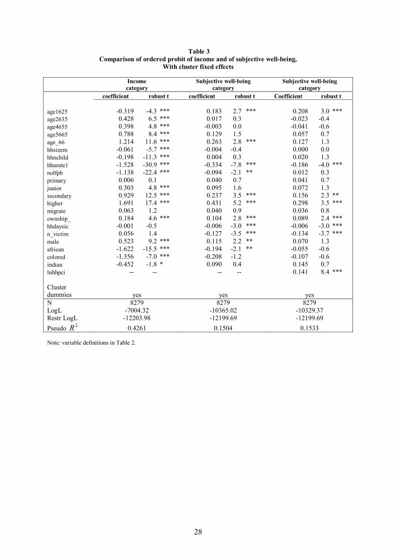
Table 3 re-estimates the income and subjective well-being equations with cluster fixed effects,

i.e. a set of cluster dummy variables. Variables that do not vary within clusters, such as

location (urban, metropol, homeland and province) and cluster characteristics such as whether

community roads become impassable at certain times of the year (impass) and whether

community is served by public transport (pubtran), are excluded from the estimation.

Including cluster fixed effects increases the explained variation in income from 38 to 43

percent and in happiness from 8 to 15 percent. Table 3 shows that apart from the effect of

race – which changes dramatically - the coefficients on unemployment, education, home

ownership, health, crime and income remain more or less unchanged with cluster fixed

effects. The fact that race coefficients collapse in size and significance suggests that race per

se is not associated with happiness (members of certain races are not intrinsically happier

than those of others) but rather that unobserved circumstances that matter to happiness differ

across the races. For instance, the huge negative coefficient on the African (and to a lesser

extent on Coloured and Indian) race dummies in Table 2 may be due to the fact that Africans

are concentrated in locations where public services and amenities – what might be termed

‘social wages’ - are very poor. While we do include certain measures of community

in the happiness equation. However, there is no strong a priori theoretical justification for them. Studies using panel data and exogenous variation in income (e.g. a lottery win) have found that causality runs from income to happiness (e.g. see Gardner and Oswald, 2001).

17

characteristics, such as whether community roads become impassable at certain times of the

year (impass) and whether public transport passes by the community (pubtran) – and also

experimented with others5 – these arguably do not capture all the relevant amenities and

services that matter to perceived well-being.

To summarise, income is the most commonly used proxy for well-being – being apparently

objective, accurately measurable and readily available – and the most commonly used

measure of poverty. However, although household per capita income is indeed positively

correlated with household subjectively evaluated well-being, the correlation is not strong.

Subjective well-being is also related to a range of non-monetary factors, including education,

employment, health and safety from crime. The ways in which these factors affect income

differ substantially from the ways in which they affect happiness. Researchers who adhere to

the income approach to poverty do so at peril of oversimplifying.

4.2 Subjective well-being poverty versus capabilities poverty?

This section examines the relationships between the subjective well-being criterion for

poverty and, within the capabilities approach, the physical functioning (or basic needs)

criterion and the social functioning (or social needs) criterion. The methodology based on

equation (1) in Section 3 allows us to attach weights to different components of physical and

social functioning to estimate their contribution to subjective well-being.

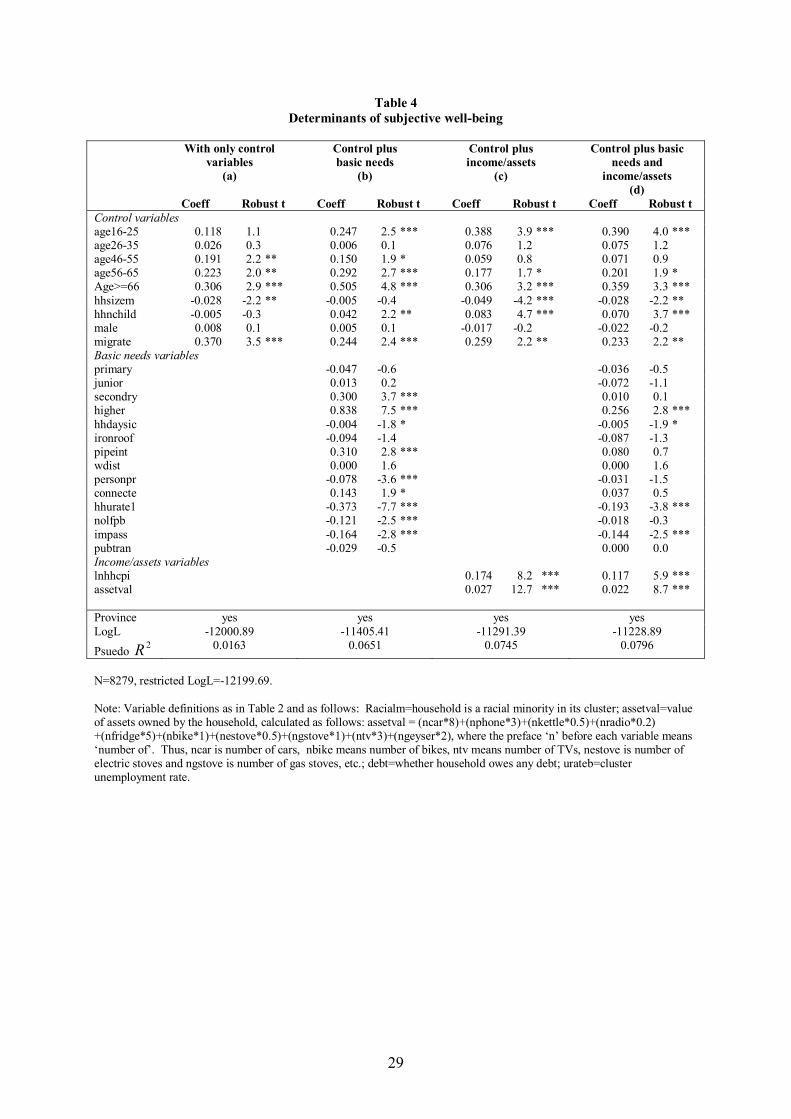
Table 4 presents ordered probits of subjective well-being. Province dummies are included in

all specifications but not reported. The first column (column a) starts with the inclusion only

of control variables, namely age, household demographics, gender and whether the household

migrated to its current location in the previous five years. Column (b) includes basic needs

variables such as education, health, employment and living conditions that can affect physical

functioning. The last set includes household variables such as distance to water (dwater),

type of house roof - ironroof (a corrugated iron roof would mean that the home is too hot in

the summer and too cold in the winter), electricity connection (connecte), and persons per

room (personpr), as well as cluster variables such as the condition of roads (impass) and 5 We experimented with variables from the cluster questionnaire including distance from the cluster to various facilities (such as health clinic, school, shops, bank, post-office, market etc.), number of such facilities within the cluster, and distance to nearest source of transport, as well as with cluster averages of household variables such as distance to nearest source of water for the household, etc.

18

whether public transport is available in community (pubtran). The inclusion of these

variables causes the pseudo R-square to rise dramatically. Almost all the basic needs

variables are statistically significant determinants of happiness.

Column (c) adds to (a) only the monetary poverty variables, i.e. income (log of household per

capita income) and wealth (value of assets owned). Both lnhhpci and assetval are important

determinants: the inclusion of these two variables raises the pseudo R-square by more than

does the set of 14 basic needs variables (column (b)).

Column (d) includes control variables together with both basic needs and income/asset

variables. The coefficient on income falls significantly compared with column (c), but

remains large and statistically highly significant. Controlling for income and assets reduces

the coefficients of the basic needs variables and renders most of them insignificant. The

physical functioning variables that have a statistically significant relationship with subjective

well-being even after controlling for monetary poverty are health, employment and condition

of community roads (which probably proxies for other community factors as well). Higher

education is the only level of education that remains significant, but that is hardly a basic

need.

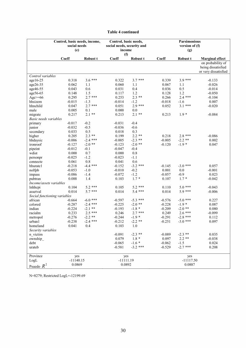
Column (e) of Table 4 adds three types of social functioning variables: race dummies

(African, Coloured, Indian – the base category being White), location dummies (urban,

metropol, and homeland) and whether the household is a racial minority in the cluster in

which it lives (racialm). In order to function socially, people must be able to relate well to

others in society. Each of these variables can affect the ability to function within the society:

race can reflect discrimination and prejudice, location can identify the type of community or

life-style to which one relates, and being a racial minority in a cluster can reflect social

disadvantage. The inclusion of the race and location variables raises the explanatory power

of the model but makes little difference to the original variables. Race is important even after

controlling for income and physical functionings. As discussed in Section 4.1, when cluster

fixed effects are used, race becomes insignificant, suggesting that here it is picking up the

effect of unobserved cluster conditions that matter to life-satisfaction. People in urban areas

and metropolitan cities are significantly less happy than those in rural areas. Households that

are racial minorities in their cluster are happier than others. This is contrary to our

19

expectation, but it is possible that racialm proxies for the high achievement among non-white

households which enables them to live in predominantly white areas.

Column (f) adds what we have termed ‘security/insecurity’ variables. These capture how

insecure the household is physically (in terms of exposure to crime, n_victim) and

economically, in terms of debt, risk of unemployment (as captured by the cluster

unemployment rate, urateb) and lack of assets that could be liquidated in time of need (home

ownership, ownship)6. Inclusion of these variables does not alter the existing coefficients,

and it raises explanatory power only modestly. The variables themselves are mostly

statistically significant, and have the expected signs: insecurity reduces subjective well-being.

A comparison of columns (c) and (f) shows that the introduction of all the other poverty

variables reduces the coefficient on log of household per capita income (lnhhpci)

substantially, from 0.174 to 0.105. It suggests that the direct influence of income is 60%, and

the indirect influence is 40%, of its total effect. However, this may exaggerate the indirect

influence of income if their association does not reflect the causal effect of income on the

other variables.

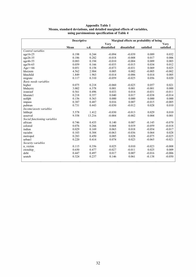
Column (g) provides our preferred, parsimonious version of column (f), together with the

marginal effects of the variables on the probability of being subjective well-being poor, i.e. of

being dissatisfied or very dissatisfied with life. The means, standard deviations and the full

set of marginal effects of the variables are shown in Appendix Table 1. If the proportion of

household members aged 16-25 increases from one standard deviation below to one standard

deviation above the mean, the probability of being in the bottom two life-satisfaction

categories falls by 7 percentage points. A rise in log of per capita household income from one

standard deviation below to one standard deviation above the mean reduces the probability of

subjective well-being poverty (i.e. of being dissatisfied or very dissatisfied with life) by 12

percentage points. Considering that overall probability of being dissatisfied/very dissatisfied

is 55%, this is not a large increase. The African probability of being subjective well-being

poor is 23 percentage points higher than that of Whites, even after controlling for observed

income, education and employment, etc. Those who live in metropolitan cities are 11

percentage points more likely to be in subjective well-being poverty than are rural-dwellers. 6 The ownship, debt and urateb variables could be included under the monetary variables category, together with income and assets, and the crime variable included under the physical functionings (basic needs) category.

20

The household’s own unemployment rate has a smaller effect on the probability of being in

the bottom two happiness categories than does the cluster unemployment rate. Going from

one standard deviation below to one standard deviation above the household unemployment

rate increases that probability by 4 percentage points but doing the same for the cluster

unemployment rate reduces it by 10 percentage points. The effects of higher education,

health, crime and debt are also small, compared with the effect of household income,

household assets, and race.

What do these results enable us to say about the relationships among the various criteria for

poverty? Subjective well-being poverty is related to both income poverty and capabilities

poverty. The comparison of the R-squares in columns (b) and (c) of Table 4 suggests that it is

somewhat better related to income poverty than it is to capabilities poverty but this may be

because our measures of capabilities poverty are imperfect. Certainly the results do not

support the notion that income poverty is an adequate measure of capabilities poverty since

variables that measure physical and social capabilities to function - such as health,

employment, mobility, and freedom from forms of insecurity - matter to happiness even after

controlling for economic factors such as income and assets. The parsimonious version of the

all-inclusive equation (column (g)) indicates that, in addition to the control variables, the

economic variables (income and assets), some physical functioning variables, some social

functioning variables and some security variables have a statistically significant influence on

subjective well-being. The subjective well-being approach to poverty is not necessarily in

competition with the other approaches. Rather, it can be viewed as an encompassing

approach which incorporates, evaluates and weights the others.

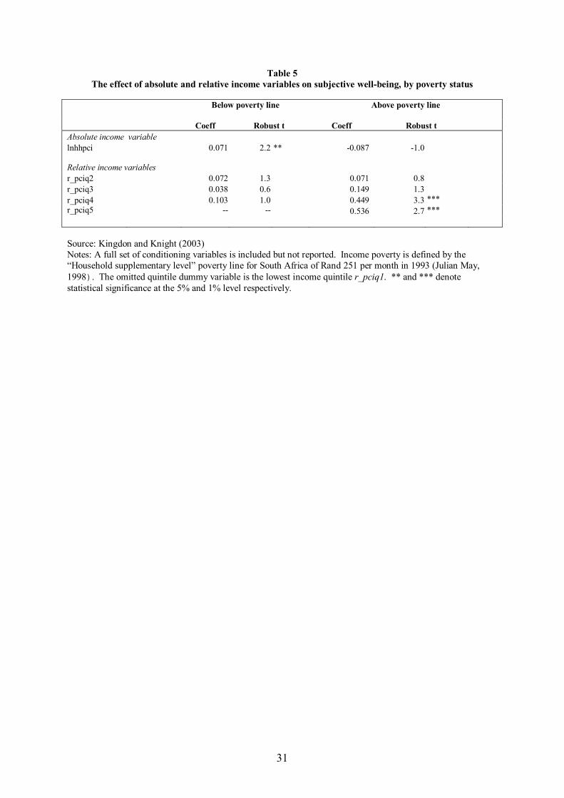
We experimented with the inclusion of both the income (lnhhpci) and also the race-specific

income quintile of the household (r_pciqj, j=1, ...5); r_pciq1, the lowest quintile being the

omitted category). Table 5 shows the results for these variables; a full set of conditioning

variables were included but are not reported. The equation was estimated for two groups: the

income-poor and the income-non-poor. There is an interesting difference between the

income-poor (who represent roughly half of the households) and the non-poor. The

coefficient on lnhhpci is significantly positive for the poor but not for the others. However,

the coefficients on the race-specific income quintiles rise monotonically, and the highest two

are highly significant, in the non-poor group, whereas there is no such relationship in the poor

group. For those in income poverty, it is absolute income that matters, whereas for others it is

21

relative income – in particular relative income within their race-group – that affects their

subjective well-being. It suggests that the need to function physically predominates when

income is low but that social functioning takes over as income rise7.

5. Conclusions

We have developed a methodology for using subjective well-being as the criterion for

poverty, and have illustrated its use by reference to a South African data set. We conclude

generally that the new research on the economics of happiness, although still in its infancy,

does indeed offer promise of successful adaptation for the analysis of poverty in poor

countries.

Our main conceptual and empirical conclusions are the following. Survey-based indicators of

subjective well-being are amenable to quantitative analysis, and can be explained in terms of

numerous socio-economic variables. There are powerful regularities to be found, both

generally and in our own illustrative analysis. This raises the possibility of using explanations

of subjective well-being to examine poverty. Any attempt to define and describe poverty

involves a value judgement as to what constitutes a good quality of life or a bad one. We

argued that an approach which examines the individual’s own perception of well-being is less

imperfect, or more quantifiable, or both, as a guide to forming that value judgement than are

the other potential approaches. Thus, we combined positive and normative analysis. We used

the positive results on the determinants of subjective well-being to infer value judgements

about the nature and components of poverty that were based on the aggregation of individual

perceptions.

In our illustrative case study we found that income and happiness are positively correlated but

that the association is not exclusive. Income enters positively and significantly into the

subjective well-being function but so also do several other variables. These include proxies

for the fulfilment of various needs which cannot normally be met by spending income. Many

of the variables that determine income also determine subjective well-being, but their effects

can differ in relative importance and even in direction.

7 Kingdon and Knight (2004) explore the effect of relative income on subjective well-being in greater detail.

22

Provided that the metric of utility is accepted as the evaluative criterion, the subjective well-

being approach to poverty does not compete with the income, capabilities and security

approaches, but rather encompasses them. Our main contribution is to view subjective well-

being as an encompassing concept, permitting us to quantify the relevance and importance of

the other approaches to poverty and of their component variables. In estimating subjective

well-being functions for South Africa we found that our preferred equation contained some

variables corresponding to the income approach, some to the basic needs (or physical

functioning) approach, some to the relative (or social functioning) approach, and some to the

security approach. Our methodology effectively provided weights of the relative importance

of these various components of subjective well-being poverty. We regard this approach as

superior to one that arbitrarily attaches weights – quite likely equal weights, for lack of a

reasoned alternative – to certain pre-selected components. Two caveats are in order. First,

the possibility that some of the explanatory variables are endogenous or causally interrelated,

and our inability of correct for these problems in this data set, means that the estimated

weights on the explanatory variables might be a somewhat misleading guide to their causal

effects on subjective well-being. Second, we would not wish to generalise from the South

African case: the possibility that different preferences across countries will generate different

sets of weights opens a new avenue of research.

23

References

Atkinson, A.B. and F. Bourguignon (1999). “Poverty and inclusion from a world perspective”, July,

typescript. Also published as “Pauvrete et inclusion dans une perspective mondiale”, Revue d'Economie du Developpement. June 2000; 0(1-2): 13-32.

Bertrand, M. and S. Mullainathan (2001). “Do people mean what they say? Implications for subjective

survey data”, Department of Economics Working Paper: 01/04, Massachusetts Institute of Technology, January.

Clark, A. (1999). “Are wages habit-forming? Evidence from micro data”, Journal of Economic

Behaviour and Organisation, June, 39: 179-200. Clark, A. (2000). “Unemployment is a social norm: Psychological evidence from panel data”, mimeo,

Orleans, France. Clark, A. and A. Oswald (1994). “Unhappiness and unemployment”, Economic Journal, 104, 648-59. Clark, David A. (2004).”Sen’s capabilities approach and the many spaces of human well-being”,

Journal of Development Studies, forthcoming.

Diener, E. and R. Biswas-Diener (2000). “New directions in subjective well-being research: The cutting edge”, mimeo, University of Illinois.

Diener, E. and R. Biswas-Diener (2003). “Findings on subjective well-being and their implications for

empowerment”, Workshop on “Measuring Empowerment: Cross-Disciplinary Perspectives”, World Bank, Washington D.C., February, 2003.

Di Tella, R., R. MacCulloch, and A. Oswald (2001). “Preferences over inflation and unemployment:

evidence from surveys of happiness”, American Economic Review, 91, 335-41. Duesenberry, James S. (1949). Income, Savings and the Theory of Consumer Behavior, Cambridge:

University of Harvard Press. Easterlin, R.A. (2001). “Income and happiness: Towards a unified theory”, Economic Journal, 111,

465-84. Frey, B. and A. Stutzer (2002). “Can economists learn from happiness research?”, Journal of

Economic Literature, XL, 2, 402-35. Gardner, J. and A. Oswald (2001). “Does money buy happiness? A longitudinal study using data on

windfalls”, mimeo, University of Warwick. Graham, C. and S. Pettinato (2002). “Frustrated achievers: Winners, losers and subjective well-being

in new market economies”, Journal of Development Studies, 38(4): 100-140. Grimard, F. (1997). “Household consumption smoothing through ethnic ties: Evidence from Cote

d’Ivoire”, Journal of Development Economics, 53: 391-422. Helliwell, John F. (2002). “How’s life? Combining individual and national variables to explain

subjective well-being”, Economic Modelling, 20: 331-60.

24

Kingdon, G. G. and J. Knight (2004). “Community, comparisons and subjective well-being in a divided society”, WPS/2004-21, Centre for the Study of African Economies, University of Oxford, June.

Laderchi, C. R., R. Saith and F. Stewart (2003). “Does it matter that we do not agree on the definition

of poverty? A comparison of four approaches”, Oxford Development Studies, 31, 3: 243-74. Layard, R. (2003a). “Happiness”, LSE Alumnus Magazine, summer, 10. Layard, R. (2003b). “Rethinking public economics: The implications of rivalry and habit”, mimeo,

Centre for Economic Performance, London School of Economics. Layard, R. (2003c). “Happiness: Has social science a clue?”, Lionel Robbins Memorial Lectures

2002/3, London School of Economics; 3, 4, 5 March. May, Julian (1998). “Poverty and inequality in South Africa”, Report prepared for the Office of the

Executive Deputy President, University of Natal. Pradhan, M. and M. Ravallion (2000). “Measuring poverty using qualitative perceptions of

consumption adequacy”, Review of Economics and Statistics, 82, 462-71. Putnam, R.D. (2001). “Social capital: measurement and consequences”, in J.F. Helliwell (ed.), The

Contribution of Human and Social Capital to Sustained Economic Growth and Well-Being, Ottawa: HRDC, forthcoming.

Ravallion , M. and M. Lokshin (2001). “Identifying welfare effects using subjective questions”,

Economica, 68, 335-57. Ravallion, M. and M. Lokshin (2002). “Self-rated economic welfare in Russia”, European Economic

Review, 46, 1453-73. Rosenzweig, M. and O. Stark (1989). “Consumption smoothing, migration and marriage: Evidence

from rural India”, Journal of Political Economy, 97(4): 905-27. Runciman, W.G. (1966). Relative Deprivation and Social Justice, Berkeley: University of California

Press. SALDRU (1994). “South Africans Rich and Poor: Baseline Household Statistics”, South African

Labour and Development Research Unit, School of Economics, University of Cape Town. August.

Sen, Amartya K. (1983). “Poor, relatively speaking”, Oxford Economic Papers, 35, 153-69. Sen, Amartya K. (1984). “Rights and capabilities”, in Resources, Values and Development, Oxford:

Basil Blackwell, 307-24. Townsend, R. (1994). “Risk and insurance in village India”, Econometrica, 62(3): 539-92. UNDP (2000). Human Development Report 2000, Oxford University Press: New York. Van Praag, B., P. Frijters and A. Ferrer-i-Carbonell (2002). “The anatomy of subjective well-being”,

Tinbergen Institute Discussion Paper No. 022/3, Amsterdam. Veenhoven, Ruut (1991). “Is happiness relative?”, Social Indicators Research, 24, 1-34.

25

Winkelmann, Liliana and Rainer Winkelmann (1998). “Why are the unemployed so unhappy? Evidence from panel data”, Economica, 65, 1-15.

26

Table 1 Cross-tabulation of subjective well-being category and income category

Subjective well-being category Income

category 1 2 3 4 5 Total

1 568 880 156 296 44 1,944 29.2 45.3 8.0 15.2 2.3 100 29.2 31.7 19.8 13.5 7.1 23.3

2 781 1,078 257 568 96 2,780

28.1 38.8 9.2 20.4 3.5 100 40.2 38.8 32.7 25.9 15.4 33.4

3 167 265 81 214 60 787

21.2 33.7 10.3 27.2 7.6 100 8.6 9.5 10.3 9.8 9.7 9.5

4 406 498 248 793 250 2,195

18.5 22.7 11.3 36.1 11.4 100 20.9 17.9 31.5 36.1 40.2 26.4

5 22 59 45 324 172 622

3.5 9.5 7.2 52.1 27.7 100 1.1 2.1 5.7 14.7 27.7 7.5 Total 1,944 2,780 787 2,195 622 8,328 23.3 33.4 9.5 26.4 7.5 100 100 100 100 100 100 100 Note: the numbers in each cell present the frequency, row percentage, and column percentage respectively.

27

Table 2 Comparison of ordered probit of income and of subjective well-being

Income

Category (a)

Subjective well-being Category

(b)

Subjective well-being Category

(c) Coefficient robust t coefficient robust t coefficient robust t age16-25 -0.421 -4.6 *** 0.216 2.5 *** 0.258 3.0 *** age26-35 0.443 6.5 *** 0.056 0.9 0.012 0.2 age46-55 0.368 5.2 *** 0.078 1.0 0.037 0.5 age56-65 0.732 7.5 *** 0.206 2.1 ** 0.132 1.3 age>=66 1.197 10.3 *** 0.379 3.6 *** 0.231 2.1 ** hhsizem -0.063 -5.0 *** -0.009 -0.7 -0.004 -0.4 hhnchild -0.196 -9.5 *** 0.017 1.0 0.035 2.0 ** hhurate1 -1.487 -23.1 *** -0.400 -8.3 *** -0.238 -4.8 *** nolfpb -1.133 -19.8 *** -0.183 -3.8 *** -0.063 -1.2 primary 0.143 2.0 ** -0.015 -0.2 -0.028 -0.4 junior 0.468 6.2 *** 0.039 0.6 -0.005 -0.1 secondary 1.158 13.1 *** 0.215 2.8 *** 0.100 1.4 higher 1.937 15.0 *** 0.523 5.4 *** 0.347 3.8 *** migrate 0.170 2.6 *** 0.229 2.0 ** 0.221 1.9 ownship_ 0.121 2.5 *** 0.104 2.4 *** 0.099 2.3 ** hhdaysic 0.001 0.2 -0.006 -2.3 ** -0.006 -2.3 ** n_victim 0.102 2.3 ** -0.074 -1.9 * -0.085 -2.2 ** male 0.680 7.6 *** 0.060 0.7 -0.012 -0.1 african -1.500 -15.2 *** -1.042 -10.4 *** -0.908 -8.9 *** colored -0.948 -8.8 *** -0.458 -4.1 *** -0.374 -3.4 *** indian -0.728 -4.8 *** -0.343 -3.3 *** -0.280 -2.8 *** metropol 0.340 3.5 *** -0.171 -1.5 -0.208 -1.8 * urban1 0.091 1.0 -0.197 -2.1 ** -0.211 -2.2 ** homeland 0.029 0.3 0.014 0.1 0.012 0.1 wcape -0.293 -3.1 *** 0.163 1.6 0.192 1.8 * ncape -0.351 -1.5 0.344 1.8 * 0.379 1.9 * ecape -0.345 -3.7 *** 0.107 0.8 0.156 1.2 natal -0.230 -2.5 ** 0.361 2.8 ** 0.385 2.9 *** ofs -0.123 -0.8 0.311 1.9 * 0.319 2.0 ** etvl 0.029 0.2 0.523 2.6 ** 0.523 2.5 *** ntvl -0.394 -4.2 *** 0.247 1.7 * 0.295 2.0 ** nw 0.113 1.0 0.307 1.6 0.299 1.5 impass -0.186 -3.4 *** -0.177 -3.0 *** -0.156 -2.6 *** pubtran 0.106 2.0 ** 0.045 0.7 0.037 0.6 lnhhpci - - - - 0.146 6.7 *** N 8279 8279 8279 LogL -7555.56 -11251.83 -11205.38 Restr LogL -12203.979 -12199.69 -12199.69 Pseudo 2R 0.3809 0.0777 0.0815 Note: The age variables= proportion of persons in each age range within the household. hhsizem = household size; hhnchild=number of children below age 16 within the household; hhurate1= household unemployment rate, i.e. proportion of household labour force participant members that are unemployed. hhurate is undefined (missing) for households with no labour force participants, so for these households, the included variable hhurate1 takes value 0 and the indicator variable nolfpb takes the value 1; nolfpb=0 for households with >=1 labour force participant; Primary, junior, secondary and higher= proportion of household members with these different levels of education; migrate=whether household migrated to its current area within the past 5 years; ownship_=whether household lives in owned home; hhdaysic=total number of person days that household members were sick in the past 14 days; n_victim=number of times in the past 12 months that household members have been victims of crime (robbery, assault, rape, murder, and abduction and ‘other’); male=proportion of males in household; African, coloured, Indian= race dummies (base category is ‘white’); metropol=household lives in metropolitan city; urban1=household in urban non-metropolitan area (base category is rural); homeland=household lives in a former ‘homeland’/Bantustan. Wcape – nw =province dummies; impass=whether community roads become impassable at certain times of the year; pubtran=whether community has public transport; lnhhpci=natural log of household per capita income.

28

Table 3 Comparison of ordered probit of income and of subjective well-being,

With cluster fixed effects Income

category Subjective well-being

category Subjective well-being

category coefficient robust t coefficient robust t Coefficient robust t age1625 -0.319 -4.3 *** 0.183 2.7 *** 0.208 3.0 *** age2635 0.428 6.5 *** 0.017 0.3 -0.023 -0.4 age4655 0.398 4.8 *** -0.003 0.0 -0.041 -0.6 age5665 0.788 8.4 *** 0.129 1.5 0.057 0.7 age_66 1.214 11.6 *** 0.263 2.8 *** 0.127 1.3 hhsizem -0.061 -5.7 *** -0.004 -0.4 0.000 0.0 hhnchild -0.198 -11.3 *** 0.004 0.3 0.020 1.3 hhurate1 -1.528 -30.9 *** -0.334 -7.8 *** -0.186 -4.0 *** nolfpb -1.138 -22.4 *** -0.094 -2.1 ** 0.012 0.3 primary 0.006 0.1 0.040 0.7 0.041 0.7 junior 0.303 4.8 *** 0.095 1.6 0.072 1.3 secondary 0.929 12.5 *** 0.237 3.5 *** 0.156 2.3 ** higher 1.691 17.4 *** 0.431 5.2 *** 0.298 3.5 *** migrate 0.063 1.2 0.040 0.9 0.036 0.8 ownship_ 0.184 4.6 *** 0.104 2.8 *** 0.089 2.4 *** hhdaysic -0.001 -0.5 -0.006 -3.0 *** -0.006 -3.0 *** n_victim 0.056 1.4 -0.127 -3.5 *** -0.134 -3.7 *** male 0.523 9.2 *** 0.115 2.2 ** 0.070 1.3 african -1.622 -15.5 *** -0.194 -2.1 ** -0.055 -0.6 colored -1.356 -7.0 *** -0.208 -1.2 -0.107 -0.6 indian -0.452 -1.8 * 0.090 0.4 0.145 0.7 lnhhpci -- -- -- -- 0.141 8.4 *** Cluster dummies yes yes yes N 8279 8279 8279 LogL -7004.32 -10365.02 -10329.37 Restr LogL -12203.98 -12199.69 -12199.69 Pseudo 2R 0.4261 0.1504 0.1533 Note: variable definitions in Table 2.

29

Table 4 Determinants of subjective well-being

With only control

variables (a)

Control plus basic needs

(b)

Control plus income/assets

(c)

Control plus basic needs and

income/assets (d)

Coeff Robust t Coeff Robust t Coeff Robust t Coeff Robust t Control variables age16-25 0.118 1.1 0.247 2.5 *** 0.388 3.9 *** 0.390 4.0 *** age26-35 0.026 0.3 0.006 0.1 0.076 1.2 0.075 1.2 age46-55 0.191 2.2 ** 0.150 1.9 * 0.059 0.8 0.071 0.9 age56-65 0.223 2.0 ** 0.292 2.7 *** 0.177 1.7 * 0.201 1.9 * Age>=66 0.306 2.9 *** 0.505 4.8 *** 0.306 3.2 *** 0.359 3.3 *** hhsizem -0.028 -2.2 ** -0.005 -0.4 -0.049 -4.2 *** -0.028 -2.2 ** hhnchild -0.005 -0.3 0.042 2.2 ** 0.083 4.7 *** 0.070 3.7 *** male 0.008 0.1 0.005 0.1 -0.017 -0.2 -0.022 -0.2 migrate 0.370 3.5 *** 0.244 2.4 *** 0.259 2.2 ** 0.233 2.2 ** Basic needs variables primary -0.047 -0.6 -0.036 -0.5 junior 0.013 0.2 -0.072 -1.1 secondry 0.300 3.7 *** 0.010 0.1 higher 0.838 7.5 *** 0.256 2.8 *** hhdaysic -0.004 -1.8 * -0.005 -1.9 * ironroof -0.094 -1.4 -0.087 -1.3 pipeint 0.310 2.8 *** 0.080 0.7 wdist 0.000 1.6 0.000 1.6 personpr -0.078 -3.6 *** -0.031 -1.5 connecte 0.143 1.9 * 0.037 0.5 hhurate1 -0.373 -7.7 *** -0.193 -3.8 *** nolfpb -0.121 -2.5 *** -0.018 -0.3 impass -0.164 -2.8 *** -0.144 -2.5 *** pubtran -0.029 -0.5 0.000 0.0 Income/assets variables lnhhcpi 0.174 8.2 *** 0.117 5.9 *** assetval 0.027 12.7 *** 0.022 8.7 *** Province yes yes yes yes LogL -12000.89 -11405.41 -11291.39 -11228.89 Psuedo 2R 0.0163 0.0651 0.0745 0.0796

N=8279, restricted LogL=-12199.69. Note: Variable definitions as in Table 2 and as follows: Racialm=household is a racial minority in its cluster; assetval=value of assets owned by the household, calculated as follows: assetval = (ncar*8)+(nphone*3)+(nkettle*0.5)+(nradio*0.2) +(nfridge*5)+(nbike*1)+(nestove*0.5)+(ngstove*1)+(ntv*3)+(ngeyser*2), where the preface ‘n’ before each variable means ‘number of’. Thus, ncar is number of cars, nbike means number of bikes, ntv means number of TVs, nestove is number of electric stoves and ngstove is number of gas stoves, etc.; debt=whether household owes any debt; urateb=cluster unemployment rate.

30

Table 4 continued Control, basic needs, income,

social needs (e)

Control, basic needs, social needs, security and

income (f)

Parsimonious version of (f)

(g)

Coeff Robust t Coeff Robust t Coeff Robust t Marginal effect

on probability of being dissatisfied

or very dissatisfied Control variables age16-25 0.318 3.6 *** 0.322 3.7 *** 0.339 3.9 *** -0.133 age26-35 0.062 1.1 0.060 1.1 0.067 1.1 -0.026 age46-55 0.043 0.6 0.031 0.4 0.036 0.5 -0.014 age56-65 0.148 1.5 0.117 1.2 0.128 1.2 -0.050 Age>=66 0.295 2.7 *** 0.253 2.3 ** 0.266 2.4 *** -0.104 hhsizem -0.015 -1.3 -0.014 -1.2 -0.018 -1.6 0.007 hhnchild 0.047 2.7 *** 0.051 2.9 *** 0.052 3.1 *** -0.020 male 0.005 0.1 0.000 0.0 migrate 0.217 2.1 ** 0.213 2.1 ** 0.213 1.9 * -0.084 Basic needs variables primary -0.017 -0.2 -0.031 -0.4 junior -0.032 -0.5 -0.036 -0.6 secondary 0.033 0.5 0.018 0.3 higher 0.205 2.3 ** 0.199 2.2 ** 0.218 2.8 *** -0.086 hhdaysic -0.006 -2.4 *** -0.005 -2.3 ** -0.005 -2.2 ** 0.002 ironroof -0.127 -2.0 ** -0.123 -2.0 ** -0.120 -1.9 * 0.047 pipeint -0.012 -0.1 -0.047 -0.4 wdist 0.000 0.7 0.000 0.8 personpr -0.025 -1.2 -0.023 -1.1 connecte 0.061 0.8 0.041 0.6 hhurate1 -0.218 -4.4 *** -0.152 -3.2 *** -0.145 -3.0 *** 0.057 nolfpb -0.053 -1.0 -0.010 -0.2 0.001 0.0 -0.001 impass -0.086 -1.4 -0.072 -1.2 -0.057 -0.9 0.023 pubtran 0.088 1.4 0.103 1.7 * 0.107 1.7 * -0.042 Income/assets variables lnhhcpi 0.104 5.2 *** 0.105 5.2 *** 0.110 5.0 *** -0.043 assetval 0.014 5.7 *** 0.014 5.4 *** 0.014 5.9 *** -0.006 Social functioning variables african -0.664 -6.0 *** -0.597 -5.3 *** -0.576 -5.0 *** 0.227 colored -0.287 -2.4 *** -0.225 -2.0 ** -0.228 -1.9 * 0.087 indian -0.224 -2.1 ** -0.193 -1.8 * -0.209 -2.0 ** 0.080 racialm 0.233 2.5 *** 0.246 2.7 *** 0.249 2.6 *** -0.099 metropol -0.276 -2.2 ** -0.244 -1.9 * -0.291 -2.8 *** 0.112 urban1 -0.238 -2.4 *** -0.212 -2.2 ** -0.251 -3.0 *** 0.097 homeland 0.041 0.4 0.103 1.0 Security variables n_victim -0.091 -2.3 ** -0.089 -2.3 ** 0.035 ownship_ 0.079 1.8 * 0.097 2.2 ** -0.038 debt -0.065 -1.6 * -0.062 -1.5 0.024 urateb -0.581 -3.2 *** -0.529 -2.7 *** 0.208 Province yes yes yes LogL -11140.15 -11111.19 -11117.50 Psuedo 2R 0.0869 0.0892 0.0887

N=8279; Restricted LogL=-12199.69

31

Table 5 The effect of absolute and relative income variables on subjective well-being, by poverty status

Below poverty line Above poverty line

Coeff Robust t Coeff Robust t Absolute income variable lnhhpci 0.071 2.2 ** -0.087 -1.0 Relative income variables r_pciq2 0.072 1.3 0.071 0.8 r_pciq3 0.038 0.6 0.149 1.3 r_pciq4 0.103 1.0 0.449 3.3 *** r_pciq5 -- -- 0.536 2.7 *** Source: Kingdon and Knight (2003) Notes: A full set of conditioning variables is included but not reported. Income poverty is defined by the “Household supplementary level” poverty line for South Africa of Rand 251 per month in 1993 (Julian May, 1998). The omitted quintile dummy variable is the lowest income quintile r_pciq1. ** and *** denote statistical significance at the 5% and 1% level respectively.

32

Appendix Table 1 Means, standard deviations, and detailed marginal effects of variables,

using parsimonious specification of Table 4 Descriptive Marginal effects on probability of being

Mean s.d. Very

dissatisfied

dissatisfied

satisfied Very

satisfied Control variables age16-25 0.198 0.244 -0.094 -0.039 0.089 0.032 age26-35 0.186 0.282 -0.018 -0.008 0.017 0.006 age46-55 0.083 0.194 -0.010 -0.004 0.009 0.003 age56-65 0.059 0.166 -0.035 -0.015 0.034 0.012 Age>=66 0.051 0.158 -0.073 -0.031 0.069 0.025 hhsizem 4.562 2.984 0.005 0.002 -0.005 -0.002 hhnchild 1.849 1.963 -0.014 -0.006 0.014 0.005 migrate 0.117 0.310 -0.059 -0.025 0.056 0.020 Basic needs variables higher 0.075 0.218 -0.060 -0.025 0.057 0.021 hhdaysic 3.002 6.378 0.001 0.001 -0.001 0.000 ironroof 0.561 0.496 0.033 0.014 -0.031 -0.011 hhurate1 0.218 0.357 0.040 0.017 -0.038 -0.014 nolfpb 0.156 0.363 0.000 0.000 0.000 0.000 impass 0.387 0.487 0.016 0.007 -0.015 -0.005 pubtran 0.731 0.443 -0.030 -0.012 0.028 0.010 Income/assets variables lnhhcpi 5.578 1.412 -0.030 -0.013 0.029 0.010 assetval 9.558 13.216 -0.004 -0.002 0.004 0.001 Social functioning variables african 0.746 0.435 0.140 0.087 -0.145 -0.070 colored 0.076 0.266 0.068 0.019 -0.059 -0.018 indian 0.029 0.169 0.063 0.018 -0.054 -0.017 racialm 0.103 0.304 -0.063 -0.036 0.064 0.028 metropol 0.283 0.450 0.085 0.028 -0.075 -0.025 urban1 0.220 0.414 0.074 0.023 -0.065 -0.021 Security variables n_victim 0.115 0.356 0.025 0.010 -0.023 -0.008 ownship_ 0.650 0.477 -0.027 -0.011 0.025 0.009 debt 0.447 0.497 0.017 0.007 -0.016 -0.006 urateb 0.324 0.237 0.146 0.061 -0.138 -0.050

33

Appendix Table 2 Subjective well-being equation with individual respondent’s personal characteristics

Parsimonious

Equation from Table 4 (a)

(a) with personal characteristics of the household respondent

(b) Coeff Robust t Coeff Robust t Control variables age16-25 0.339 3.9 *** 0.267 2.9 *** age26-35 0.067 1.1 0.020 0.3 age46-55 0.036 0.5 0.084 1.1 age56-65 0.128 1.2 0.200 1.8 * Age>=66 0.266 2.4 *** 0.331 2.7 *** hhsizem -0.018 -1.6 -0.012 -1.0 hhnchild 0.052 3.1 *** 0.044 2.5 *** migrate 0.213 1.9 * 0.218 2.0 ** Basic needs variables higher 0.218 2.8 *** 0.250 2.8 *** hhdaysic -0.005 -2.2 ** -0.005 -2.2 ** ironroof -0.120 -1.9 * -0.114 -1.8 * hhurate1 -0.145 -3.0 *** -0.140 -2.7 *** nolfpb 0.001 0.0 0.013 0.2 impass -0.057 -0.9 -0.062 -1.0 pubtran 0.107 1.7 * 0.111 1.8 * Income/assets variables lnhhcpi 0.110 5.0 *** 0.115 5.1 *** assetval 0.014 5.9 *** 0.015 6.2 *** Social functioning variables african -0.576 -5.0 *** -0.566 -5.0 *** colored -0.228 -1.9 * -0.210 -1.8 * indian -0.209 -2.0 ** -0.197 -1.9 * racialm 0.249 2.6 *** 0.247 2.6 *** metropol -0.291 -2.8 *** -0.300 -2.8 *** urban1 -0.251 -3.0 *** -0.255 -3.2 *** Security variables n_victim -0.089 -2.3 ** -0.092 -2.3 ** ownship_ 0.097 2.2 ** 0.099 2.3 ** debt -0.062 -1.5 -0.061 -1.5 urateb -0.529 -2.7 *** -0.542 -2.8 *** r_age -0.010 -1.9 * r_agesq 0.000 1.3 r_edyrs -0.006 -0.5 r_edyrsq 0.000 0.1 r_male -0.021 -0.6 r_empld 0.003 0.1 Province yes yes LogL -11117.50 -10984.71 Restr LogL -12199.69 -12063.84 Psuedo 2R 0.0887 0.0895 N 8279 8190

Note: r_age and r_agesq are respondent’s age and its square; r_edyrs and r_edyrsq are respondent’s years of education and its square; r_male is gender and r_empld whether the respondent is employed or not.

34

W

X

W = W1(X, a)

W = W2(X)

W = W1(X, c)

a

d

b

c

W’

W’’

X’ X’’

Figure 1