Multi-scale flow simulation of automotive catalytic converters

Cansu Ozhan, Daniel Fuster n, Patrick Da CostaCNRS (UMR 7190), Université Pierre et Marie Curie, Institut Jean le Rond d'Alembert, 4 place Jussieu, 75252, Paris Cedex 05, France

H I G H L I G H T S

� We model the flow occurring at multiple scales inside catalytic converters.� A subgrid model is proposed for the flow in the monolith channels.� Adaptive Mesh Refinement techniques are optimized to capture the main flow features.� The new model is validated against the experimental results reported by Benjamin.� The new model allows for significant computational time savings compared to the full simulation.

a r t i c l e i n f o

Article history:Received 3 December 2013Received in revised form24 March 2014Accepted 30 April 2014Available online 14 May 2014

Keywords:Catalytic convertersComputational fluid dynamicsAdaptive mesh refinementFlow mal-distribution

a b s t r a c t

The flow distribution within the automotive catalytic converter is an important controlling factor on theoverall conversion efficiency. Capturing the flow features minimizing the computational cost is the firstimportant step towards the solution of the complex full engineering problem. In this work we present anovel approach that combines physical and numerical multi-resolution techniques in order to correctlycapture the flow features inside an automotive catalytic converter. While Adaptive Mesh Refinementtechniques are optimized in order to minimize the computational effort in the divergent region, a novelsubgrid model is developed to describe the flow inside the catalytic substrate placed between theconvergent and divergent regions. The proposed Adaptive Mesh Refinement methods are tested for twotest cases representative of the flow features found in the divergent region of a catalytic converter. Theperformance of the new subgrid model is validated against the non-uniformity index and the radialvelocity profile data obtained by Benjamin et al. (2002). The effective coupling of AMR techniques andthe subgrid model significantly reduces the error of the numerical predictions to 5–15% in conditionswhere the full simulation of the problem is out of current computational capabilities.

& 2014 Elsevier Ltd. All rights reserved.

1. Introduction

Transportation is responsible for a large part of global emissions(Pachauri and Reisinger, 2007). This problematic has led to govern-ments to establish very stringent conditions for the maximumemissions levels. Post-treatment systems need to be further devel-oped in order to meet with these emissions requirements.A large part of the current studies is devoted to find efficient catalyststo improve the reaction efficiency, but one can also optimize theperformance of these equipments by acting on the flow distributioninside the catalytic converter. A few studies (Agrawal et al., 2012;Bella et al., 1991; Guojiang and Song, 2005; Karvounis and Assanis,1993) have focused on the flow distribution effect on the conversionefficiency. However, the interaction between flow and conversionefficiency has not yet been understood completely.

In an ideal situation, the flow at the converter inlet is uniform.However, in practical cases, high Reynolds numbers, pulsatingflow, abrupt expansion, and the impact of porous media lead tonon-homogeneous and non-uniform velocity profiles at the inletconverter. Because the velocity profile is non-uniform, we finddifferent inlet velocities (hence different mass flow rates) in thesubstrate monolith channels. This results in premature degrada-tion of the catalyst in areas of high flow rates and poor volumeutilization of catalyst in areas of low flow rates, which turns intoa decrease of the system's efficiency (Benjamin et al., 2002;Karvounis and Assanis, 1993). The flow inside the system underthese physical and geometrical effects generates large range ofscales on the flow in addition to the molecular scales inherent ofthe chemical reactions that occur inside the catalytic medium.Capturing all the physics and chemistry inside the system is out ofreach for the available computational capabilities (Nien et al.,2013; Siemund et al., 1996).

The development of numerical tools and models is crucialin order to optimize the performance of catalytic converters

Contents lists available at ScienceDirect

journal homepage: www.elsevier.com/locate/ces

Chemical Engineering Science

http://dx.doi.org/10.1016/j.ces.2014.04.0440009-2509/& 2014 Elsevier Ltd. All rights reserved.

n Corresponding author.E-mail address: fuster@dalembert.upmc.fr (D. Fuster).

Chemical Engineering Science 116 (2014) 161–171

(Chatterjee et al., 2002; Tischer et al., 2001; Tischer andDeutschmann, 2005). Modeling approaches for automotive cata-lytic converters have presented by Pontikakis et al. (2004). Thesetools must be capable of predicting the effect of externallycontrolled variables in the flow distribution. The simulation ofthe entire system is not simple due to all the complex transportand chemical phenomena that take place inside the system. Thus,the large range of lengthscales involved in the process makes thefull solution of the basic equations far beyond current availablecomputational capabilities. As an alternative, we can resort toreliable models and specific multi-resolution techniques in orderto investigate the process (Charpentier, 2005). These models aimat providing a better understanding of the system's responseto externally controlled variables (e.g. inlet velocities, effect ofgeometry, etc.) keeping a low computational cost.

In this work we develop and test multi-resolution numericaltechniques and models to capture the main physical process takingplace inside automotive catalyst systems. In particular we focusthis work on the development of numerical techniques andmodels to correctly capture the characteristics of the flow createdinside these systems in order to establish a solid base on whichimplement chemical reaction models. We propose a subgridmodel for the flow inside the catalytic substrate which is coupledwith the full solution of the Navier–Stokes equations in thediffuser and convergent regions, where Adaptative Mesh Refine-ment (AMR) techniques are optimized to minimize the computa-tional cost. A free CFD package (Gerris) is used as a platform toimplement the models (Popinet, 2003, 2009).

Adaptative Mesh Refinement is a numerical technique toconcentrate the computational effort on regions where the flowproperties vary dramatically, coarsening the regions where theflow properties variations are small (Hauke et al., 2008; Popinet,2003). These techniques have been already shown significantcomputational time savings in problems involving liquid atomiza-tion (Fuster et al., 2009b, 2013) and other multiphase flow studies(Fuster et al., 2009a). In this work we investigate the capability ofAMR to reduce the computational limitations related to the DirectNumerical Simulation (DNS) of turbulent flows typically foundinside catalytic converter systems. Various authors have tried toexplore the capabilities of AMR techniques for the particularproblem of turbulent flow simulations (Bockhorn et al., 2009;Gao and Groth, 2006, 2010; Nazarov and Hoffman, 2013). Some ofthese methods, despite their accuracy, suffer of being exceedinglycomputationally expensive which impedes their application to realproblems. This fact strengthens the compromise that one has toreach between accuracy and computational effort. Turbulentsimulations usually have related long simulation runs in order toobtain reproducible statistics of the flow of interest. Thus, in thiswork we focus on AMR techniques whose computational cost isnegligible compared to the cost related to the numerical solutionof the flow equations.

In this study, the general problem is presented first, then thederivation of a simplified model for the flow in catalytic substrateis developed. The accuracy of the model is demonstrated by

comparing the results with the full simulation of the flow in thisregion. Then, we focus our efforts in deriving efficient AdaptiveMesh Refinement methods for the flow characteristics typicallyfound in the divergent region (e.g. recirculation regions and shearlayer). The accuracy and efficiency of the method is verifiedagainst related test cases with analytical solution. The new modelis validated against the experimental data reported by Benjaminet al. (2002). Finally, we present a full numerical example of atypical automotive catalyst system.

2. Problem formulation

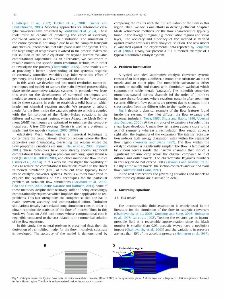
A typical and ideal automotive catalytic converter systemsconsist of an inlet pipe, a diffuser, a monolithic substrate, an outletnozzle and an outlet pipe. The monolithic substrate is eitherceramic or metallic and coated with aluminium washcoat whichsupports the noble metals (catalysts). The monolith comprisesnumerous parallel narrow channels (of the order of 1 mm) toincrease the surface area where reactions occur. In after-treatmentsystems, different flow patterns are present due to changes in thecross section from the diffuser inlet to the nozzle outlet.

Fig. 1 depicts a classical example of the flow features foundinside the system. In the inlet diffuser the flow expands andbecomes turbulent (Neve, 1993; Shuja and Habib, 1996; Ubertiniand Desideri, 2000). At the entrance of expansion a turbulent freeshear layer develops. A main flow jet region appears close to theaxis of symmetry whereas a recirculation flow region appearsright after the beginning of the expansion. The intense recircula-tion induces high energy dissipation rates within the separatedflow region (Forrester and Evans, 1997). The flow within thecatalytic channel is significantly simpler. The flow is laminarizedby viscous forces inside the narrow channels that induce asignificant pressure drop across the channel compared to inletdiffuser and outlet nozzle. The characteristic Reynolds numbersin this region do not exceed 500 (Karvounis and Assanis, 1993).Finally, at the outlet nozzle, the section contracts and we find swirlflow (Forrester and Evans, 1997).

In the next subsections, the governing equations and models tosolve these equations are discussed in detail.

3. Governing equations

3.1. Full model

The incompressible fluid assumption is widely used in theliterature for the simulation of the flow in catalytic converters(Chakravarthy et al., 2003; Guojiang and Song, 2005; Holmgrenet al., 1997; Lai et al., 1992). Treating the exhaust gas as incom-pressible fluid is a reasonable approximation since the Machnumber is smaller than 0.05, acoustic waves have a negligibleimpact (Chakravarthy et al., 2003) and the variations in pressureare less than 10% of the absolute pressure (Holmgren et al., 1997).

Fig. 1. Catalytic converter. Typical flow patterns inside a catalytic converter (Re¼10,000) in the symmetric plane. A shear layer and a large recirculation region are observedin the diffuser region. The flow is re-laminarized inside the catalytic channels.

C. Ozhan et al. / Chemical Engineering Science 116 (2014) 161–171162

For the sake of simplicity, we assume that the temperature changein the system is not significant and hence the fluid properties areconstant. Under these assumptions and considering the gas as aNewtonian fluid, the governing equations for the flow are

∇ � u¼ 0; ð1Þ

ρ∂u∂t

þu � ∇u� �

¼ �∇pþμ∇2uþS: ð2Þ

where t is the time, u is the velocity, ρ is the fluid density, p is thepressure, μ is the viscosity and S is a momentum source term.

In addition, when chemical reactions inside the system need tobe modeled, we have to add N transport equations, being N thenumber of components present in the system. For the ith compo-nent we write

∂ci∂t

¼∇ � ðD∇ciÞ�∇ � ðuciÞþRi ð3Þ

where ci is the concentration of the ith component, D is thediffusion coefficient and Ri is the reaction rate.

These equations can be solved by imposing proper boundaryconditions. Typically we assume that the velocity at the inlet isknown and we apply a classical outflow boundary condition at theoutlet section (Dirichlet boundary condition for pressure andNeumann boundary condition for the normal velocity). Thevelocity at the solid walls is imposed equal to zero.

As stated above, the full solution of these equations is exceed-ingly expensive and we need to propose simplified solutionstrategies that we apply in regions where the flow features arealready well captured by simple models. In particular, the flowinside the catalytic converter is a good candidate for such models.In the next subsection, we present the approach considered tomodel the flow in this region and how the model is coupled to thefull numerical solution of the Navier–Stokes in the diffuser andconvergent regions.

3.2. Subgrid models

3.2.1. Pressure drop model for monolithic channelsThe flow inside monolithic channels is usually a fully developed

laminar flow where the averaged velocity is kept constant by massconservation. In these conditions, the pressure drop inside thechannel is mainly induced by viscous forces and the flow is knownto be well represented by the Hagen–Poiseuille pressure dropmodel (Heck et al., 2001)

Δp¼ 32Rec

Ldρu2; ð4Þ

where Rec is the Reynolds number inside the channel defined withthe channel diameter d and L is the channel length.

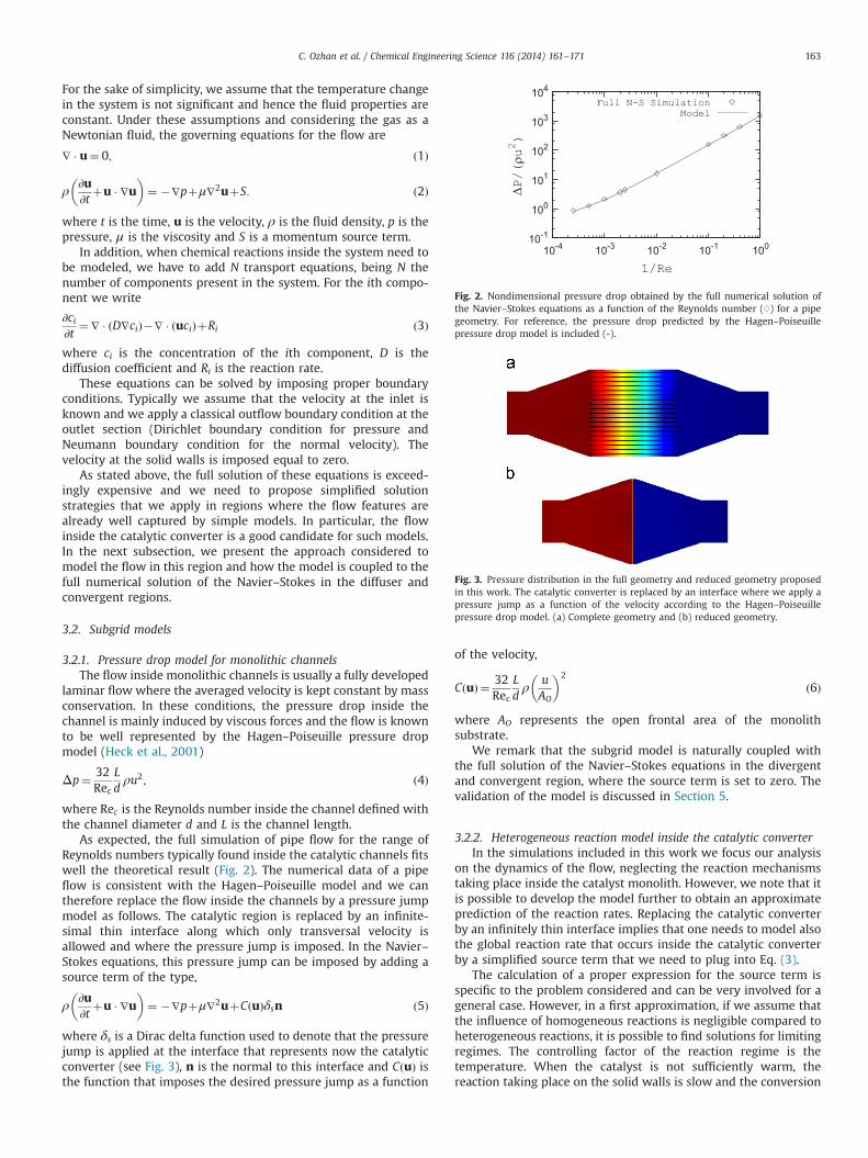
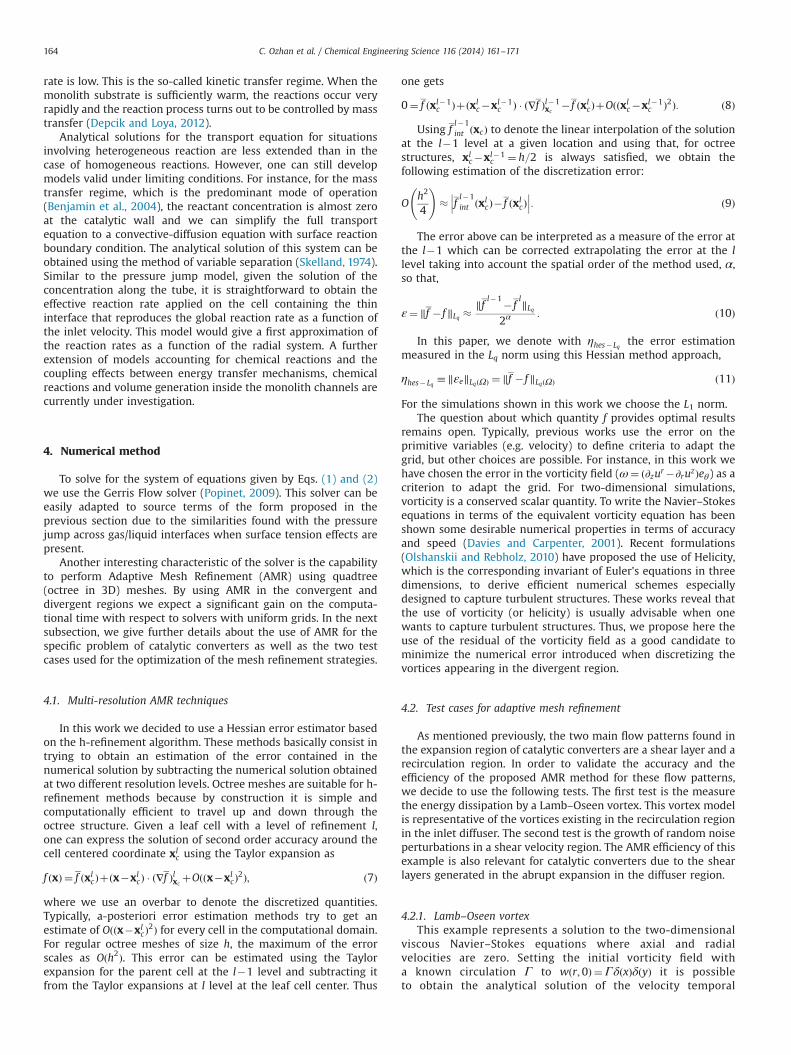
As expected, the full simulation of pipe flow for the range ofReynolds numbers typically found inside the catalytic channels fitswell the theoretical result (Fig. 2). The numerical data of a pipeflow is consistent with the Hagen–Poiseuille model and we cantherefore replace the flow inside the channels by a pressure jumpmodel as follows. The catalytic region is replaced by an infinite-simal thin interface along which only transversal velocity isallowed and where the pressure jump is imposed. In the Navier–Stokes equations, this pressure jump can be imposed by adding asource term of the type,

ρ∂u∂t

þu � ∇u� �

¼ �∇pþμ∇2uþCðuÞδsn ð5Þ

where δs is a Dirac delta function used to denote that the pressurejump is applied at the interface that represents now the catalyticconverter (see Fig. 3), n is the normal to this interface and CðuÞ isthe function that imposes the desired pressure jump as a function

of the velocity,

CðuÞ ¼ 32Rec

Ldρ

uAO

� �2

ð6Þ

where AO represents the open frontal area of the monolithsubstrate.

We remark that the subgrid model is naturally coupled withthe full solution of the Navier–Stokes equations in the divergentand convergent region, where the source term is set to zero. Thevalidation of the model is discussed in Section 5.

3.2.2. Heterogeneous reaction model inside the catalytic converterIn the simulations included in this work we focus our analysis

on the dynamics of the flow, neglecting the reaction mechanismstaking place inside the catalyst monolith. However, we note that itis possible to develop the model further to obtain an approximateprediction of the reaction rates. Replacing the catalytic converterby an infinitely thin interface implies that one needs to model alsothe global reaction rate that occurs inside the catalytic converterby a simplified source term that we need to plug into Eq. (3).

The calculation of a proper expression for the source term isspecific to the problem considered and can be very involved for ageneral case. However, in a first approximation, if we assume thatthe influence of homogeneous reactions is negligible compared toheterogeneous reactions, it is possible to find solutions for limitingregimes. The controlling factor of the reaction regime is thetemperature. When the catalyst is not sufficiently warm, thereaction taking place on the solid walls is slow and the conversion

10-1

100

101

102

103

104

10-4 10-3 10-2 10-1 100

ΔP/(ρ u

2)

1/Re

Full N-S SimulationModel

Fig. 2. Nondimensional pressure drop obtained by the full numerical solution ofthe Navier–Stokes equations as a function of the Reynolds number (♢) for a pipegeometry. For reference, the pressure drop predicted by the Hagen–Poiseuillepressure drop model is included (-).

Fig. 3. Pressure distribution in the full geometry and reduced geometry proposedin this work. The catalytic converter is replaced by an interface where we apply apressure jump as a function of the velocity according to the Hagen–Poiseuillepressure drop model. (a) Complete geometry and (b) reduced geometry.

C. Ozhan et al. / Chemical Engineering Science 116 (2014) 161–171 163

rate is low. This is the so-called kinetic transfer regime. When themonolith substrate is sufficiently warm, the reactions occur veryrapidly and the reaction process turns out to be controlled by masstransfer (Depcik and Loya, 2012).

Analytical solutions for the transport equation for situationsinvolving heterogeneous reaction are less extended than in thecase of homogeneous reactions. However, one can still developmodels valid under limiting conditions. For instance, for the masstransfer regime, which is the predominant mode of operation(Benjamin et al., 2004), the reactant concentration is almost zeroat the catalytic wall and we can simplify the full transportequation to a convective-diffusion equation with surface reactionboundary condition. The analytical solution of this system can beobtained using the method of variable separation (Skelland, 1974).Similar to the pressure jump model, given the solution of theconcentration along the tube, it is straightforward to obtain theeffective reaction rate applied on the cell containing the thininterface that reproduces the global reaction rate as a function ofthe inlet velocity. This model would give a first approximation ofthe reaction rates as a function of the radial system. A furtherextension of models accounting for chemical reactions and thecoupling effects between energy transfer mechanisms, chemicalreactions and volume generation inside the monolith channels arecurrently under investigation.

4. Numerical method

To solve for the system of equations given by Eqs. (1) and (2)we use the Gerris Flow solver (Popinet, 2009). This solver can beeasily adapted to source terms of the form proposed in theprevious section due to the similarities found with the pressurejump across gas/liquid interfaces when surface tension effects arepresent.

Another interesting characteristic of the solver is the capabilityto perform Adaptive Mesh Refinement (AMR) using quadtree(octree in 3D) meshes. By using AMR in the convergent anddivergent regions we expect a significant gain on the computa-tional time with respect to solvers with uniform grids. In the nextsubsection, we give further details about the use of AMR for thespecific problem of catalytic converters as well as the two testcases used for the optimization of the mesh refinement strategies.

4.1. Multi-resolution AMR techniques

In this work we decided to use a Hessian error estimator basedon the h-refinement algorithm. These methods basically consist intrying to obtain an estimation of the error contained in thenumerical solution by subtracting the numerical solution obtainedat two different resolution levels. Octree meshes are suitable for h-refinement methods because by construction it is simple andcomputationally efficient to travel up and down through theoctree structure. Given a leaf cell with a level of refinement l,one can express the solution of second order accuracy around thecell centered coordinate xl

c using the Taylor expansion as

f ðxÞ ¼ f ðxlcÞþðx�xl

cÞ � ð∇f ÞlxcþOððx�xl

cÞ2Þ; ð7Þ

where we use an overbar to denote the discretized quantities.Typically, a-posteriori error estimation methods try to get anestimate of Oððx�xl

cÞ2Þ for every cell in the computational domain.For regular octree meshes of size h, the maximum of the errorscales as Oðh2Þ. This error can be estimated using the Taylorexpansion for the parent cell at the l�1 level and subtracting itfrom the Taylor expansions at l level at the leaf cell center. Thus

one gets

0¼ f ðxl�1c Þþðxl

c�xl�1c Þ � ð∇f Þl�1

xc� f ðxl

cÞþOððxlc�xl�1

c Þ2Þ: ð8Þ

Using fl�1int ðxcÞ to denote the linear interpolation of the solution

at the l�1 level at a given location and using that, for octreestructures, xl

c�xl�1c ¼ h=2 is always satisfied, we obtain the

following estimation of the discretization error:

Oh2

4

!� f

l�1int ðxl

cÞ� f ðxlcÞ���:��� ð9Þ

The error above can be interpreted as a measure of the error atthe l�1 which can be corrected extrapolating the error at the llevel taking into account the spatial order of the method used, α,so that,

ε¼ ‖f � f ‖Lq �‖f

l�1� fl‖Lq

2α: ð10Þ

In this paper, we denote with ηhes� Lq the error estimationmeasured in the Lq norm using this Hessian method approach,

ηhes�Lq � ‖εe‖LqðΩÞ ¼ ‖f � f‖LqðΩÞ ð11Þ

For the simulations shown in this work we choose the L1 norm.The question about which quantity f provides optimal results

remains open. Typically, previous works use the error on theprimitive variables (e.g. velocity) to define criteria to adapt thegrid, but other choices are possible. For instance, in this work wehave chosen the error in the vorticity field (ω¼ ð∂zur�∂ruzÞeθ) as acriterion to adapt the grid. For two-dimensional simulations,vorticity is a conserved scalar quantity. To write the Navier–Stokesequations in terms of the equivalent vorticity equation has beenshown some desirable numerical properties in terms of accuracyand speed (Davies and Carpenter, 2001). Recent formulations(Olshanskii and Rebholz, 2010) have proposed the use of Helicity,which is the corresponding invariant of Euler's equations in threedimensions, to derive efficient numerical schemes especiallydesigned to capture turbulent structures. These works reveal thatthe use of vorticity (or helicity) is usually advisable when onewants to capture turbulent structures. Thus, we propose here theuse of the residual of the vorticity field as a good candidate tominimize the numerical error introduced when discretizing thevortices appearing in the divergent region.

4.2. Test cases for adaptive mesh refinement

As mentioned previously, the two main flow patterns found inthe expansion region of catalytic converters are a shear layer and arecirculation region. In order to validate the accuracy and theefficiency of the proposed AMR method for these flow patterns,we decide to use the following tests. The first test is the measurethe energy dissipation by a Lamb–Oseen vortex. This vortex modelis representative of the vortices existing in the recirculation regionin the inlet diffuser. The second test is the growth of random noiseperturbations in a shear velocity region. The AMR efficiency of thisexample is also relevant for catalytic converters due to the shearlayers generated in the abrupt expansion in the diffuser region.

4.2.1. Lamb–Oseen vortexThis example represents a solution to the two-dimensional

viscous Navier–Stokes equations where axial and radialvelocities are zero. Setting the initial vorticity field witha known circulation Γ to wðr;0Þ ¼ΓδðxÞδðyÞ it is possibleto obtain the analytical solution of the velocity temporal

C. Ozhan et al. / Chemical Engineering Science 116 (2014) 161–171164

evolution as (Meunier and Villermaux, 2003)

uθ ¼Γ2πr

1�exp � r2

4νt

� �� �: ð12Þ

where ν is the kinematic viscosity and r and θ are respectivelythe radial and the azimuthal coordinates. A characteristiclength for this problem can be obtained by setting the radialdistance at which the velocity norm is maximal,

lc ¼ 2:2418ffiffiffiffiffiffiffiνt0

p: ð13Þ

For the simulations contained in this section we chooseνt0 ¼ 0:5 in order to define a characteristic length different fromzero. In addition, we set the circulation equal to Γ ¼ 1 in a squaredomain with nondimensional length L=lc ¼ 600 where we imposeNeumman boundary conditions for the velocity at all boundaries.

The initial velocity field is initialized according to Eq. (12). Fig. 4represents the theoretical azimuthal velocity profiles as a functionof the radius for different times. We note that the theoreticalsolution extends to infinity. This fact introduces a certain error atthe domain boundaries when setting the domain size to a finitedistance. This error cannot be attributed to the discretizationmethod and therefore, cannot be captured by the error estimator.To solve this problem, we decide to measure the efficiency of theerror estimators in a circular region of radius Rc=lc ¼ 100.

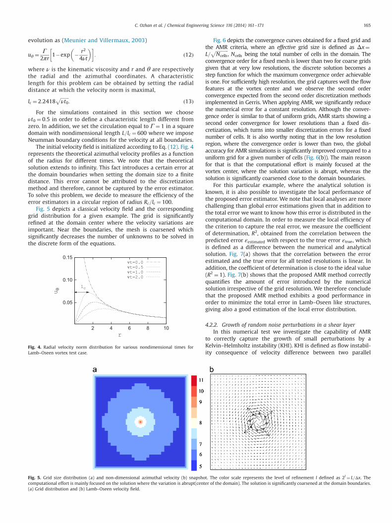
Fig. 5 depicts a classical velocity field and the correspondinggrid distribution for a given example. The grid is significantlyrefined at the domain center where the velocity variations areimportant. Near the boundaries, the mesh is coarsened whichsignificantly decreases the number of unknowns to be solved inthe discrete form of the equations.

Fig. 6 depicts the convergence curves obtained for a fixed grid andthe AMR criteria, where an effective grid size is defined as Δx¼L=

ffiffiffiffiffiffiffiffiffiffiffiNcells

p, Ncells being the total number of cells in the domain. The

convergence order for a fixed mesh is lower than two for coarse gridsgiven that at very low resolutions, the discrete solution becomes astep function for which the maximum convergence order achievableis one. For sufficiently high resolution, the grid captures well the flowfeatures at the vortex center and we observe the second orderconvergence expected from the second order discretization methodsimplemented in Gerris. When applying AMR, we significantly reducethe numerical error for a constant resolution. Although the conver-gence order is similar to that of uniform grids, AMR starts showing asecond order convergence for lower resolutions than a fixed dis-cretization, which turns into smaller discretization errors for a fixednumber of cells. It is also worthy noting that in the low resolutionregion, where the convergence order is lower than two, the globalaccuracy for AMR simulations is significantly improved compared to auniform grid for a given number of cells (Fig. 6(b)). The main reasonfor that is that the computational effort is mainly focused at thevortex center, where the solution variation is abrupt, whereas thesolution is significantly coarsened close to the domain boundaries.

For this particular example, where the analytical solution isknown, it is also possible to investigate the local performance ofthe proposed error estimator. We note that local analyses are morechallenging than global error estimations given that in addition tothe total error we want to know how this error is distributed in thecomputational domain. In order to measure the local efficiency ofthe criterion to capture the real error, we measure the coefficientof determination, R2, obtained from the correlation between thepredicted error εestimated with respect to the true error εtrue, whichis defined as a difference between the numerical and analyticalsolution. Fig. 7(a) shows that the correlation between the errorestimated and the true error for all tested resolutions is linear. Inaddition, the coefficient of determination is close to the ideal value(R2 ¼ 1). Fig. 7(b) shows that the proposed AMR method correctlyquantifies the amount of error introduced by the numericalsolution irrespective of the grid resolution. We therefore concludethat the proposed AMR method exhibits a good performance inorder to minimize the total error in Lamb–Oseen like structures,giving also a good estimation of the local error distribution.

4.2.2. Growth of random noise perturbations in a shear layerIn this numerical test we investigate the capability of AMR

to correctly capture the growth of small perturbations by aKelvin–Helmholtz instability (KHI). KHI is defined as flow instabil-ity consequence of velocity difference between two parallel

0.05

0.10

0.15

2 4 6 8 10

uθ

r

lc

νt=0.0νt=0.5νt=1.0νt=2.0

Fig. 4. Radial velocity norm distribution for various nondimensional times forLamb–Oseen vortex test case.

Fig. 5. Grid size distribution (a) and non-dimensional azimuthal velocity (b) snapshot. The color scale represents the level of refinement l defined as 2l ¼ L=Δx. Thecomputational effort is mainly focused on the solution where the variation is abrupt(center of the domain). The solution is significantly coarsened at the domain boundaries.(a) Grid distribution and (b) Lamb–Oseen velocity field.

C. Ozhan et al. / Chemical Engineering Science 116 (2014) 161–171 165

streams of different velocity and/or density. This mechanism isusually encountered in a relatively large number of process leadingto the development of fully turbulent flows, such as the abruptexpansion in the diffuser region of the catalytic converter. In thispaper we investigate the temporal evolution of small perturba-tions in a baseflow profile given by

U ¼ΔUerf ðy=δcÞ; ð14Þwhere δc is the boundary layer thickness. In this configuration, it ispossible to solve for the linearized Navier–Stokes equations to findthe theoretical growthrate as a function of the wavelength. Theexact value used in this test case is obtained using the codedeveloped by Otto et al. (2013) already tested and validated for theinvestigation of perturbation growth in shear layers. The theore-tical growthrate ci as a function of the wavelength α tends to thefollowing asymptotic value when the Reynolds number is infi-nitely large

αmδc ¼ 0:5ðαciÞmδcΔU

¼ 0:215737 ð15Þ

In order to reproduce these results, a simulation domain of size½Lx=δc; Ly=δc� ¼ ½100;300� is considered where ΔU and δc are takenas the characteristic velocity and length of the problem (Fig. 8(a)).

Random noise of low amplitude is initially imposed on top ofthe baseflow profile in order to excite all the possible wavelengths.The noise is introduced through a random source on the Navier–Stokes equation in the y direction modulated with a Gaussiandistribution

S¼ RandðÞe�y2 tΔUδc

r1: ð16Þ

The source is switched off for larger times.

A measure of the perturbation growth can be obtained bymeasuring the maximum amplitude of the vertical velocity V intime. In particular, Fig. 8(b) depicts the temporal evolution of the Vcomponent of the velocity integrated across the entire domain.After an initial transient state, the instability develops and gen-erates well resolved structures that grow in time exponentially(Fig. 8(c)–(e)). The numerical growth-rate is obtained by fitting theperturbation growth in a time interval tΔU=δc ¼ ½30 : 50�. Theerror is then computed by comparing the numerical and theore-tical growthrate.

Fig. 9 depicts an example of the grid distribution typicallygenerated. The grid is significantly refined at the velocity shearregion where the velocity variations are important and it iscoarsened gradually as variations become less important.

Fig. 10 shows the error in the growth-rate obtained for auniform mesh and a non-uniform mesh adapted according to theHessian error estimator in the vorticity field. As in the previoustest case, the AMR grid provides more accurate than a fixed meshfor a given resolution (Fig. 10). AMR is able to start displayingsecond order convergence for lower resolutions given that it isable to concentrate the grid cells in those regions where the erroris large. For coarse grids the convergence order is significantlydegraded but in any case the AMR provides significantly moreaccurate solutions than a fixed grid for a fixed number of cells(Fig. 10(b)).

5. Validation of the subgrid pressure jump model

In this section we concentrate on the validation of the pressurejump model using the experiments presented by Benjamin (2003)and Benjamin et al. (2002), where only the expansion stage and

10 -7

10-6

10-5

10-4

10-3

10-2

101 102 103 104

ε L1(u)

lc/Δx

FIXEDAMR 1.0

101 102 103 104

(Ek)num/(Ek)theo

lc/Δx

FIXEDAMR

Fig. 6. Error convergence (a) and converged value (b) with a fixed and AMR mesh for the Lamb–Oseen vortex test case. For AMR simulations, the equivalent grid size isdefined as Δx¼ L=

ffiffiffiffiffiffiffiffiffiffiffiNcells

p. (a) Error convergence of x component of velocity based on norm L1 and (b) convergence of kinetic energy Ek on the circular region of radius

Rc=lc ¼ 100.

10-7

10-6

10-5

10-4

10-3

10-2

10-7 10-6 10-5 10-4 10-3 10-2

ε true

εestimated

0.1

1

10

101 102 103

R2

lc/Δx

ideal caseAMR

Fig. 7. Local error efficiency measurements for the Lamb–Oseen vortex test case. (a) Predicted error εestimated versus true error εtrue for all the resolutions tested and(b) coefficient of determination as a function of the grid resolution.

C. Ozhan et al. / Chemical Engineering Science 116 (2014) 161–171166

the monolith substrate region are considered. These works weredevoted to examine the flow distribution in automotive catalystsystems and to provide experimental data for verification ofcomputational fluid dynamic simulations. The experimental set-up consists of a diffuser and a substrate. The diffuser is axiallysymmetric with a total angle 601 and length 61.5 mm. The inletpipe diameter on which Reynolds number are based is 48 mm. Thevelocity profiles are measured 45 mm upstream of the diffuserthroat. A tube is used to hold flow straighteners to achieve uniformflow. Two ceramic substrates of different lengths are used(152 mm and 102 mm respectively). Both substrates have a nom-inal cell density of 400 cspi made of square channels of 1 mm. Thediameter of both substrates is 118 mm. Physical and geometricalproperties of the experimental set-up are indicated in Table 2.

During the numerical investigations, we impose a uniformvelocity profile at the inlet pipe. The walls of the system are

treated as impermeable solid walls with no-slip boundary condi-tion. For the outlet section, an outflow boundary condition isapplied.

To evaluate the effect of geometry and mass flow rate on theflow distribution a non-uniformity index sV is defined using thevariance of the velocity profile across a transversal section withrespect to the averaged uniform velocity profile

sV ¼ 1_m

ZAUi�Ue δ _m:

���� ð17Þ

The non-uniformity index over the cross section of the substrate, ψis defined as

ψ ¼sV

Ue� 100: ð18Þ

Fig. 9. Grid size distribution, velocity vectors and perturbation isolines (V) for the instability growth in a shear layer. Grid cells preferentially concentrate on the velocityshear layer region. (a) Grid distribution for the instability growth in a shear layer. The color scale represents the level of refinement l defined as 2l ¼ L=Δx and (b) zoom intothe shear layer region.

-3.0

-2.0

-1.0

0.0

1.0

2.0

3.0

-1.0 0.0 1.0

y/δ c

U/ΔU

-28-26-24-22-20-18-16-14-12-10

0 10 20 30 40 50 60

Amplitude

t(ΔU/δc)

SimulationTheory

Fig. 8. Inviscid vortex test case. A random perturbation is imposed in a shear layer. The small perturbation initially imposed in the solution grows in time creating coherentstructures corresponding to the most unstable mode for which a theoretical growthrate can be obtained. (a) Shear velocity profile, (b) temporal evolution of the amplitudedisturbance integrated over the whole domain, (c) perturbed field at tΔU=δc ¼ 0, (d) perturbed field at tΔU=δc ¼ 10, and (e) perturbed field at tΔU=δc ¼ 50.

C. Ozhan et al. / Chemical Engineering Science 116 (2014) 161–171 167

This number increases as the flow becomes less uniformly dis-tributed. For a perfectly distributed flow this number is zero.

Fig. 11 compares the vorticity fields obtained at various times.The flow patterns observed in the divergent region are similar tothose observed by Benjamin (2003). The model is able to act as aporous wall that induces strong recirculation in the expansionregion without the necessity to explicitly simulate the flow insidethe monolith channels.

To validate the developed numerical tool we measure the non-uniformity index ψ as a function of the Reynolds number for thetwo monolith substrates tested in Benjamin et al. (2002). We startshowing the convergence of the results for the monolith of length152 mm for Re¼20,000, 60,000, 80,000. As shown in Fig. 12 themodel converges to a value relatively close to the experimentalobservations for all Reynolds numbers tested here. These resultsshow that the AMR method allows us to obtain relatively accurateresults with approximately 100 times less number of grid cellscompared to a fixed mesh. The computational gain increases as theReynolds increase. The reason for this effect is that the character-istic scales of the flow become smaller as the Reynolds increases

and therefore, the efficiency of AMR increases for low resolutionsimulations.

Although the results provided by the model converge to a valuerelatively close to the experimental observations, we system-atically observe that simulation results under-predict the experi-mental value for experimental conditions. To gain further insightabout the source of this disagreement, we perform a systematiccomparison of the non-uniformity index ψ for the two differentsubstrates and as a function of the Reynolds number. Even thoughthe simulation results are consistent with the experimentalresults, Fig. 13 shows that as the substrate length decreases, theaccuracy of the model decreases too. This effect is importantfor short monoliths and high Reynolds numbers. This reveals alimitation of the pressure jump model: while the model assumes afully developed laminar flow inside the channels, in real condi-tions there is certainly a transition region at the channels entrancein which the pressure lost is not correctly captured by the Hagen–Poiseuille pressure drop model. As expected, as the length of thechannels increases it is less important the transition region on thetotal pressure drop and the model predictions become moreaccurate. The accuracy of the solution is also larger as the Reynoldsnumber decreases. At any event, we can conclude that theaccuracy of the numerical model is satisfactory given the signifi-cant amount of computational time save with respect to the costthat would be implicated in the simulation of the flow inside thechannels.

A finer analysis about the source of discrepancy betweennumerical and experimental results shows that the thickness ofthe boundary layer at the inlet has an impact on the resultsobtained. For instance, Fig. 14 compares the experimental andnumerical velocity radial distribution for Re¼79,900 assumingthat the velocity profile at the inlet pipe corresponds to

UðyÞ ¼ U0 erf �y�Rinlet

δ

� �; ð19Þ

where δ is the boundary layer thickness at the inlet pipe. Thisparameter is important given that it controls the growthrate of theinstability, which finally has an impact on the flow distributiondownstream. The value of δ that provides the best fitting betweensimulation and experimental results is δ¼5 mm. In this case,numerical results converge to the velocity profile given byBenjamin et al. (2002) as we reduce the tolerance of the AMRcriterion (Table 3). Unfortunately, the boundary layer thickness isnot explicitly given in Benjamin et al. (2002), which means thatthe numerical fitting of δ may hide errors introduced by themodels used and also by the discretization method. In any case,the good fitting between numerical and experimental results isremarkable due to the low number of grid points used and thelarge Reynolds number tested.

Table 1Simulation conditions used to test the subgrid model in Fig. 11.

Dimensions of the solution domain

Pipe diameter (Din) 50 mmPipe throughout a monolith substrate length 75 mmCatalyst diameter (Dmax) 100 mmCatalyst length 100 mmReduced catalyst length in simulation 5 mmCatalyst channel diameter 2 mm

Reynolds number at inlet pipe diameter (Re) 10,000Inlet velocity profile Uniform

Table 2Simulation of experimental set-up.

Dimensions of the geometry

Inlet pipe diameter 48 mmInlet pipe length 45 mmDiffuser length 61.5 mmTotal diffuser angle 601Substrate diameter 118 mmSubstrate length 152–102 mmNominal substrate cell density 400 cpsi

Fluid properties

Reynolds number at inlet pipe diameter (Re) 20,000–100,000Inlet velocity profile Uniform

10-4

10-3

10-2

10-1

100

10-2 10-1 100 101

ε(αci)

(δc/Δx)

FIXEDAMR

0.1

1.0

10-2 10-1 100 101

(αci)num/(αci)theo

(δc/Δx)

FIXEDAMR

Fig. 10. Error convergence (a) and converged values (b) with a fixed and AMR mesh for the instability growth in a shear layer. For AMR, the equivalent grid size is obtained asΔx¼ ffiffiffiffiffiffiffiffiffiffiffiffiffiffiffiffiffiffiffiffiffiffiffiffiffiffiffiffi

Lx � Ly=Ncellsp

. (a) Error convergence of αci and (b) converged value of αci .

C. Ozhan et al. / Chemical Engineering Science 116 (2014) 161–171168

6. Numerical example

As an example of the capabilities of the developed models andnumerical tools we present in this section the simulation resultsobtained for the simulation conditions included in Table 1 forusing the whole geometry. The characteristic length of the systemis chosen to be substrate diameter Dmax.

All simulations were performed on a Dell Precision T5500Westmere with a processor of Two Intel Xeon E5645 and totalmemory of 48 Go.

Fig. 15(a) depicts a sequence of snapshots of the resulting griddistribution obtained by vorticity based Hessian estimator. Thegrid is preferentially concentrated in the recirculation region,where most of the energy dissipation occurs (Fig. 15(b)) andwhere it is important to capture the flow features if one wantsto correctly predict the flow distribution inside the differentcatalytic converter channels.

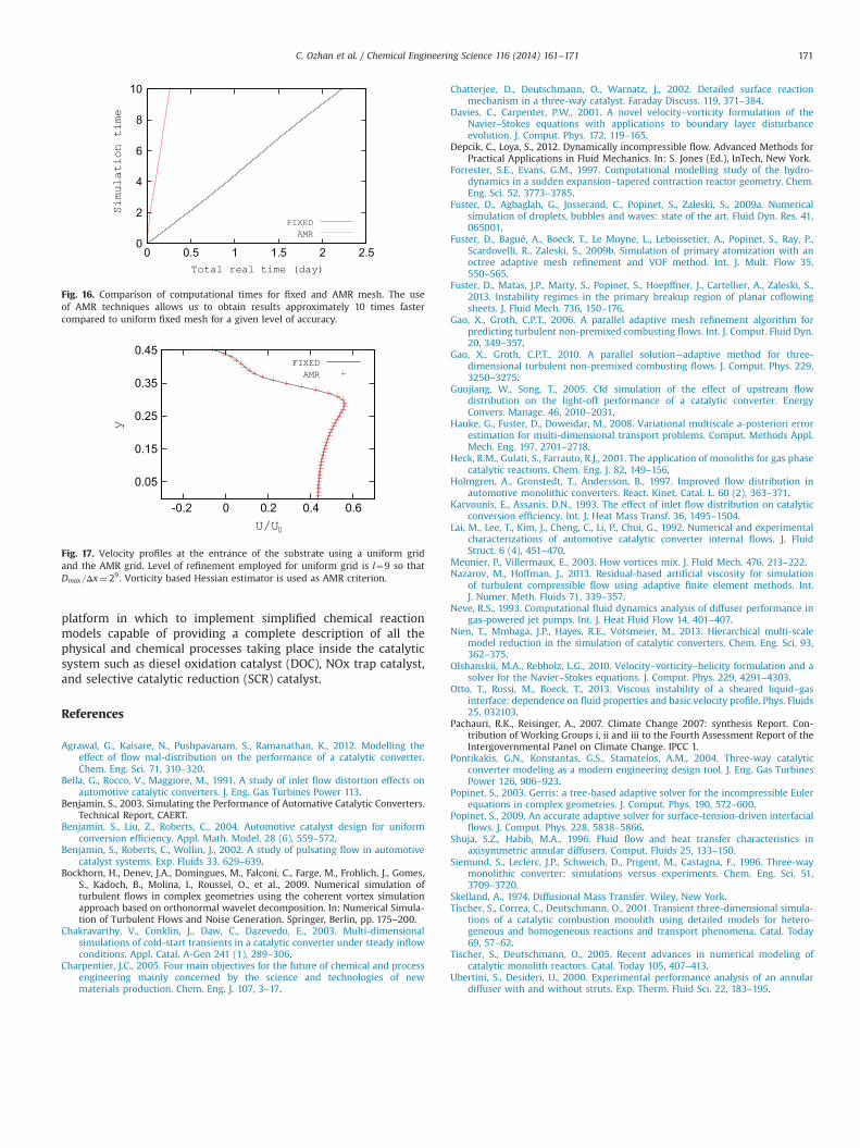
The combined use of the pressure drop model and AMRtechniques significantly reduce the computational time (Fig. 16).We emphasize that this gain is expected to be even moresignificant in full three dimensional computations. The save incomputational time is not at expenses of accuracy. As shown in

Fig. 17 the velocity profiles at the medium plane obtained for thefull numerical simulation and the simplified geometry match well.As it can be seen in Figs. 11 and 15(b) the reduced model capturesremarkably well the influence of the substrate on the flowpatterns upstream. The results are consistent with the flowpatterns observed from the full simulation considering the sub-strate (Fig. 1) and also the flow patterns observed experimentallyby Benjamin (2003).

7. Conclusion

In this paper we investigate a novel technique to couple the fullsolution of the Navier–Stokes equations in the divergent andconvergent regions of a catalytic converter with a simplifiedphysical model for the catalytic substrate.

The introduction of a new source term in the momentumequation allows us to capture the pressure drop induced by thecatalytic substrate in the flow without the need of simulating theflow inside the catalytic channels. The model has been validatedagainst the experimental results reported by Benjamin et al.(2002). The model still captures the influence of the substrate onthe main flow features observed upstream saving a significantcomputational time.

In addition to the model for the catalytic substrate, specificmulti-resolution techniques have been developed and validatedagainst test cases related to the flow features observed in thediffuser region of catalytic converter systems. We conclude that byoptimizing the grid distribution we can accelerate the simulationtime by factor 10. This factor is expected to be larger for threedimensional computations.

To sum up, the coupling of models for the flow inside thecatalytic substrate and the use of adaptive mesh refinementcombined with efficient criteria for mesh adaptation produceoptimum grid distributions that make possible to simulate com-plex flow problems involving different lengthscales in reasonablecomputational times. This work is currently being used as a solid

Fig. 11. Sequence of vorticity snapshots obtained with the pressure jump model. Diffuser and substrate properties are as shown in Table 1. The Reynolds number based oninlet pipe diameter is 10,000. The model is able to capture the effect of the substract on the flow upstream and to block the pass of vortices throughout the catalytic region asobserved in the full simulation (Fig. 1) and experimental observations from Benjamin (2003).

1

10

103 104 105 106Non-uniformity index

Degree of freedom

ExperimentalSimulation, AMR

Simulation, FIXED 1

10

103 104 105 106Non-uniformity index

Degree of freedom

ExperimentalSimulation, AMR

Simulation, FIXED 1

10

103 104 105 106Non-uniformity index

Degree of freedom

ExperimentalSimulation, AMR

Simulation, FIXED

Fig. 12. Convergence tendencies of different grid designs at different regimes. (a) Re¼20,000, (b) Re¼60,000, and (c) Re¼80,000.

0 10 20 30 40 50 60 70 80 90

100 110 120

0 20000 40000 60000 80000 100000Non-uniformity index

Reynolds number

Experimental, 152mmExperimental, 102mm

Simulation, 152mmSimulation, 102mm

Fig. 13. Non-uniformity for different regimes and substrate lengths.

C. Ozhan et al. / Chemical Engineering Science 116 (2014) 161–171 169

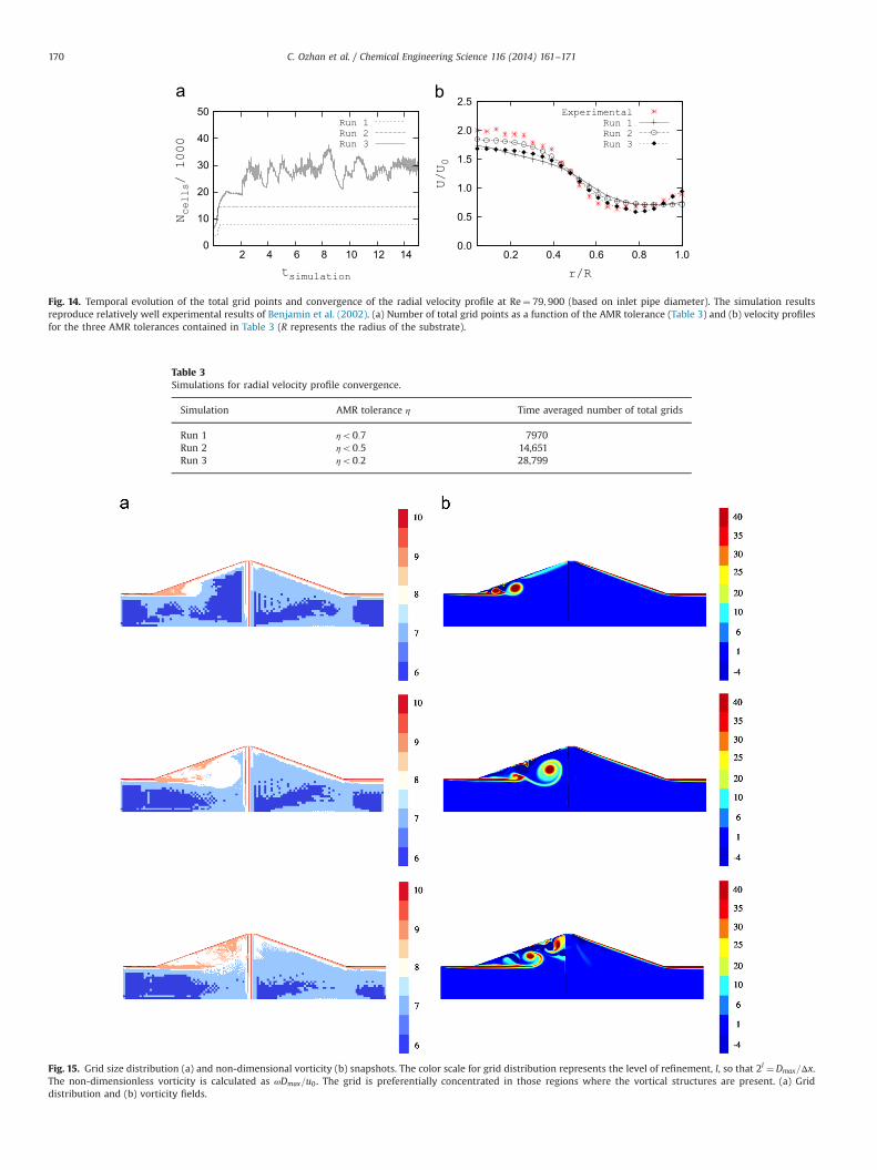
Fig. 15. Grid size distribution (a) and non-dimensional vorticity (b) snapshots. The color scale for grid distribution represents the level of refinement, l, so that 2l ¼Dmax=Δx.The non-dimensionless vorticity is calculated as ωDmax=u0. The grid is preferentially concentrated in those regions where the vortical structures are present. (a) Griddistribution and (b) vorticity fields.

0

10

20

30

40

50

2 4 6 8 10 12 14

Ncells/ 1000

tsimulation

Run 1Run 2Run 3

0.0

0.5

1.0

1.5

2.0

2.5

0.2 0.4 0.6 0.8 1.0

U/U0

r/R

ExperimentalRun 1Run 2Run 3

Fig. 14. Temporal evolution of the total grid points and convergence of the radial velocity profile at Re¼ 79;900 (based on inlet pipe diameter). The simulation resultsreproduce relatively well experimental results of Benjamin et al. (2002). (a) Number of total grid points as a function of the AMR tolerance (Table 3) and (b) velocity profilesfor the three AMR tolerances contained in Table 3 (R represents the radius of the substrate).

Table 3Simulations for radial velocity profile convergence.

Simulation AMR tolerance η Time averaged number of total grids

Run 1 ηo0:7 7970Run 2 ηo0:5 14,651Run 3 ηo0:2 28,799

C. Ozhan et al. / Chemical Engineering Science 116 (2014) 161–171170

platform in which to implement simplified chemical reactionmodels capable of providing a complete description of all thephysical and chemical processes taking place inside the catalyticsystem such as diesel oxidation catalyst (DOC), NOx trap catalyst,and selective catalytic reduction (SCR) catalyst.

References

Agrawal, G., Kaisare, N., Pushpavanam, S., Ramanathan, K., 2012. Modelling theeffect of flow mal-distribution on the performance of a catalytic converter.Chem. Eng. Sci. 71, 310–320.

Bella, G., Rocco, V., Maggiore, M., 1991. A study of inlet flow distortion effects onautomotive catalytic converters. J. Eng. Gas Turbines Power 113.

Benjamin, S., 2003. Simulating the Performance of Automative Catalytic Converters.Technical Report, CAERT.

Benjamin, S., Liu, Z., Roberts, C., 2004. Automotive catalyst design for uniformconversion efficiency. Appl. Math. Model. 28 (6), 559–572.

Benjamin, S., Roberts, C., Wollin, J., 2002. A study of pulsating flow in automotivecatalyst systems. Exp. Fluids 33, 629–639.

Bockhorn, H., Denev, J.A., Domingues, M., Falconi, C., Farge, M., Frohlich, J., Gomes,S., Kadoch, B., Molina, I., Roussel, O., et al., 2009. Numerical simulation ofturbulent flows in complex geometries using the coherent vortex simulationapproach based on orthonormal wavelet decomposition. In: Numerical Simula-tion of Turbulent Flows and Noise Generation. Springer, Berlin, pp. 175–200.

Chakravarthy, V., Conklin, J., Daw, C., Dazevedo, E., 2003. Multi-dimensionalsimulations of cold-start transients in a catalytic converter under steady inflowconditions. Appl. Catal. A-Gen 241 (1), 289–306.

Charpentier, J.C., 2005. Four main objectives for the future of chemical and processengineering mainly concerned by the science and technologies of newmaterials production. Chem. Eng. J. 107, 3–17.

Chatterjee, D., Deutschmann, O., Warnatz, J., 2002. Detailed surface reactionmechanism in a three-way catalyst. Faraday Discuss. 119, 371–384.

Davies, C., Carpenter, P.W., 2001. A novel velocity–vorticity formulation of theNavier–Stokes equations with applications to boundary layer disturbanceevolution. J. Comput. Phys. 172, 119–165.

Depcik, C., Loya, S., 2012. Dynamically incompressible flow. Advanced Methods forPractical Applications in Fluid Mechanics. In: S. Jones (Ed.), InTech, New York.

Forrester, S.E., Evans, G.M., 1997. Computational modelling study of the hydro-dynamics in a sudden expansion–tapered contraction reactor geometry. Chem.Eng. Sci. 52, 3773–3785.

Fuster, D., Agbaglah, G., Josserand, C., Popinet, S., Zaleski, S., 2009a. Numericalsimulation of droplets, bubbles and waves: state of the art. Fluid Dyn. Res. 41,065001.

Fuster, D., Bagué, A., Boeck, T., Le Moyne, L., Leboissetier, A., Popinet, S., Ray, P.,Scardovelli, R., Zaleski, S., 2009b. Simulation of primary atomization with anoctree adaptive mesh refinement and VOF method. Int. J. Mult. Flow 35,550–565.

Fuster, D., Matas, J.P., Marty, S., Popinet, S., Hoepffner, J., Cartellier, A., Zaleski, S.,2013. Instability regimes in the primary breakup region of planar coflowingsheets. J. Fluid Mech. 736, 150–176.

Gao, X., Groth, C.P.T., 2006. A parallel adaptive mesh refinement algorithm forpredicting turbulent non-premixed combusting flows. Int. J. Comput. Fluid Dyn.20, 349–357.

Gao, X., Groth, C.P.T., 2010. A parallel solution—adaptive method for three-dimensional turbulent non-premixed combusting flows. J. Comput. Phys. 229,3250–3275.

Guojiang, W., Song, T., 2005. Cfd simulation of the effect of upstream flowdistribution on the light-off performance of a catalytic converter. EnergyConvers. Manage. 46, 2010–2031.

Hauke, G., Fuster, D., Doweidar, M., 2008. Variational multiscale a-posteriori errorestimation for multi-dimensional transport problems. Comput. Methods Appl.Mech. Eng. 197, 2701–2718.

Heck, R.M., Gulati, S., Farrauto, R.J., 2001. The application of monoliths for gas phasecatalytic reactions. Chem. Eng. J. 82, 149–156.

Holmgren, A., Gronstedt, T., Andersson, B., 1997. Improved flow distribution inautomotive monolithic converters. React. Kinet. Catal. L. 60 (2), 363–371.

Karvounis, E., Assanis, D.N., 1993. The effect of inlet flow distribution on catalyticconversion efficiency. Int. J. Heat Mass Transf. 36, 1495–1504.

Lai, M., Lee, T., Kim, J., Cheng, C., Li, P., Chui, G., 1992. Numerical and experimentalcharacterizations of automotive catalytic converter internal flows. J. FluidStruct. 6 (4), 451–470.

Meunier, P., Villermaux, E., 2003. How vortices mix. J. Fluid Mech. 476, 213–222.Nazarov, M., Hoffman, J., 2013. Residual-based artificial viscosity for simulation

of turbulent compressible flow using adaptive finite element methods. Int.J. Numer. Meth. Fluids 71, 339–357.

Neve, R.S., 1993. Computational fluid dynamics analysis of diffuser performance ingas-powered jet pumps. Int. J. Heat Fluid Flow 14, 401–407.

Nien, T., Mmbaga, J.P., Hayes, R.E., Votsmeier, M., 2013. Hierarchical multi-scalemodel reduction in the simulation of catalytic converters. Chem. Eng. Sci. 93,362–375.

Olshanskii, M.A., Rebholz, L.G., 2010. Velocity–vorticity–helicity formulation and asolver for the Navier–Stokes equations. J. Comput. Phys. 229, 4291–4303.

Otto, T., Rossi, M., Boeck, T., 2013. Viscous instability of a sheared liquid–gasinterface: dependence on fluid properties and basic velocity profile. Phys. Fluids25, 032103.

Pachauri, R.K., Reisinger, A., 2007. Climate Change 2007: synthesis Report. Con-tribution of Working Groups i, ii and iii to the Fourth Assessment Report of theIntergovernmental Panel on Climate Change. IPCC 1.

Pontikakis, G.N., Konstantas, G.S., Stamatelos, A.M., 2004. Three-way catalyticconverter modeling as a modern engineering design tool. J. Eng. Gas TurbinesPower 126, 906–923.

Popinet, S., 2003. Gerris: a tree-based adaptive solver for the incompressible Eulerequations in complex geometries. J. Comput. Phys. 190, 572–600.

Popinet, S., 2009. An accurate adaptive solver for surface-tension-driven interfacialflows. J. Comput. Phys. 228, 5838–5866.

Shuja, S.Z., Habib, M.A., 1996. Fluid flow and heat transfer characteristics inaxisymmetric annular diffusers. Comput. Fluids 25, 133–150.

Siemund, S., Leclerc, J.P., Schweich, D., Prigent, M., Castagna, F., 1996. Three-waymonolithic converter: simulations versus experiments. Chem. Eng. Sci. 51,3709–3720.

Skelland, A., 1974. Diffusional Mass Transfer. Wiley, New York.Tischer, S., Correa, C., Deutschmann, O., 2001. Transient three-dimensional simula-

tions of a catalytic combustion monolith using detailed models for hetero-geneous and homogeneous reactions and transport phenomena. Catal. Today69, 57–62.

Tischer, S., Deutschmann, O., 2005. Recent advances in numerical modeling ofcatalytic monolith reactors. Catal. Today 105, 407–413.

Ubertini, S., Desideri, U., 2000. Experimental performance analysis of an annulardiffuser with and without struts. Exp. Therm. Fluid Sci. 22, 183–195.

0

2

4

6

8

10

0 0.5 1 1.5 2 2.5

Simulation time

Total real time (day)

FIXEDAMR

Fig. 16. Comparison of computational times for fixed and AMR mesh. The useof AMR techniques allows us to obtain results approximately 10 times fastercompared to uniform fixed mesh for a given level of accuracy.

0.05

0.15

0.25

0.35

0.45

-0.2 0 0.2 0.4 0.6

y

U/U0

FIXEDAMR

Fig. 17. Velocity profiles at the entrance of the substrate using a uniform gridand the AMR grid. Level of refinement employed for uniform grid is l¼9 so thatDmax=Δx¼ 29. Vorticity based Hessian estimator is used as AMR criterion.

C. Ozhan et al. / Chemical Engineering Science 116 (2014) 161–171 171