3D characterization of microstructure evolution of cast AlMgSi alloys by synchrotron tomography

CHARACTERIZATION OF MICROSTRUCTURE AND INTERNAL
DISPLACEMENT FIELD OF SAND USING
X-RAY COMPUTED TOMOGRAPHY
By
MOHAMMAD REZA RAZAVI
A dissertation submitted in partial fulfillment of the requirements for the degree of
DOCTOR OF PHILOSOPHY
WASHINGTON STATE UNIVERSITY Department of Civil and Environmental Engineering
December 2006

To the Faculty of Washington State University:
The members of the Committee appointed to examine the dissertation of
MOHAMMAD REZA RAZAVI find it satisfactory and recommend that it be accepted.
______________________________________ Chair
______________________________________
______________________________________
______________________________________
ii

ACKNOWLEDGEMENTS
First and foremost I wish to thank my advisor, Professor Muhunthan for his
support, patience, guidance, friendship, and encouragement from the first day that I
applied for the PhD program at Washington State University. While I was writing the
thesis, he gave me the moral support and freedom I needed to move on.
I would like to thank all of my thesis committee members, Professor Stephen
Antolovich, Professor Hussein Zbib, and Professor Adrian Rodriguez-Marek for their
continuous support and their helpful comments. Special thanks to Professor Stephen
Antolovich for all his friendship, kindness, help, and support from the first day I met him.
I also would like to thank Professor David Field for all of his kindness and help.
Many people at Washington State University helped me through my studies and
provided a pleasant environment for me, which I will always remember and be thankful
for. I would like to thank Maureen Clausen, Larissa Morton, Kathy Cox, Glenda Rogers,
Vickie Ruddick, Lola Gillespie, Cyndi Whitmore, Mary Furnari, Roslyn Carlson, Kevin
Emerson, Tom Weber, Bill Elliott, Jon Grimes, and Robert Lentz.
I would like to thank two great friends, Larissa Morton and Cyndi Whitmore, who
have always been there for my wife and me during the most difficult times.
I would like to thank my wife, Morvarid, for all she has done to help me reach my
goals. Without her support, help and sacrifices, it would not be possible for me to
accomplish this study.
My parents, brothers and sister have always supported me and provided me the
best in my life and I will always be thankful to them all.
iii

I would like to thank Professor Omar Al Hatamleh for all his help and
encouragement. Professor William Clocksin, Professor Larry Lake, and Professor
Michael Dennis, helped me by providing very useful information for my research and I
would like thank them.
I also would like to thank all of my friends and colleagues at Washington State
University for their kindness and their cooperation.
Steve Schramm, Anthony Davis, and Tony Melton, from HYTEC, helped me to
learn the X-ray CT and assisted with every problem I had with X-ray CT, and I would
like to thank them.
Daniel Eaton, from British Columbia University, provided me fast 3-D
normalized cross correlation code in MATLAB. It was a great help to reduce the analysis
time and I appreciate his kindness.
I would like to thank Professor Nasser Talebbeydokhti, from Civil Engineering
Department at Shiraz Engineering University, who did a great job allowing me to
continue my studies at Washington State University.
Professor Hamid Seyyedian, a great friend and teacher from Civil Engineering
Department at Shiraz Engineering University, who helped and supported me in following
my dreams and encouraging me to never give up. I am always thankful to him.
I would like to thank Professor Arsalan Ghahramani, Professor Ghassem
Habibagahi, Professor Nader Hataf, and the other Professors in Civil Engineering
Department at Shiraz Engineering University, for all their kindness and support.
Financial support by the National Science Foundation and Civil Engineering
Department at Washington State University is gratefully acknowledged.
iv

CHARACTERIZATION OF MICROSTRUCTURE AND INTERNAL
DISPLACEMENT FIELD OF SAND USING
X-RAY COMPUTED TOMOGRAPHY
Abstract
by Mohammad Reza Razavi, Ph.D.
Washington State University December 2006
Chair: Balasingam Muhunthan
This study presents a systematic method to examine the microstructure
characteristics and internal displacement field of sands using X-ray computed
tomography (CT) images. The 3-D images of spherical glass beads, Silica sand, and
Ottawa sand are characterized using advanced image processing techniques.
An interactive computer program is developed to study porosity variation with
increasing radius of a spherical volume from the 3-D images of these materials. The
porosity variation of Silica sand and Ottawa sand shows three characteristic regions: an
initial fluctuation region due to microscopic variations, a constant plateau region, and a
region with a monotonic increase/decrease due to heterogeneity. The homogenous
medium of glass beads did not show the last region. The results show that for the
spherical glass beads the representative elementary volume radius is about 2 to 3 times
the average diameter. The radius for Silica sand composed mainly of elongated particles
is between 5 to 11 times of d50 and for Ottawa sand composed mainly of subrounded
particles is between 9 to 16 times of d50. These values appear to justify the use of 10 to 20
diameters of sand grains adopted in some past studies.
v
A novel triaxial system is designed to facilitate the characterization of the 3-D
images of soil microstructure and its evolution nondestructively in real time using X-ray
computed tomography while it is subjected to shearing. The system was designed to have
a total weight of 500 N, capable to increase the cell pressure up to 400 kPa, and applying
up to 10 kN axial load. Moreover, the system is designed to be able to do temperature
controlled (-10 to 65 °C) triaxial and uniaxial tests on many different materials, including
soil, asphalt concrete, wood, small metal specimens, and composites. The system is fully
microprocessor controlled using a workstation outside of the protection cabinet of X-ray
CT. Load can be kept constant, or applied either in strain control or stress control.
A computer code is developed to determine the internal displacement field in
sands by comparing two successive X-ray CT images. The method is an extension of the
template matching technique used in image processing for 3-D situations. The program
is verified by applying a known displacement or rotation to the reference image. An
interactive computer program is developed to find the changes in local porosity
distribution within the sand specimen as it is subjected to shearing. The ability to
quantify the internal displacement and local porosity would contribute in the
characterization of strain localization and shear band development.
vi

TABLE OF CONTENTS
Page
Acknowledgements............................................................................................................ iii
Abstract ................................................................................................................................v
Table of Contents.............................................................................................................. vii
List of Figures .................................................................................................................... xi
List of Tables ................................................................................................................... xvi
Chapter 1: INTRODUCTION................................................................................................... 1
1.1 Introduction....................................................................................................... 1
1.2 Objectives ......................................................................................................... 4
1.3 Organization of the Thesis ................................................................................ 4
Chapter 2: BACKGROUND.................................................................................................... 6
2.1 Introduction....................................................................................................... 6
2.2 Determination of Representative Elementary Volume using X-ray CT........... 6
2.3 Triaxial and X-ray CT for Real Time Monitoring ............................................ 7
2.4 Internal Displacement Fields using X-ray and X-Ray CT................................ 9
2.5 Experimental Observations and Characterization of Shear Bands in Sands... 10
Chapter 3: REPRESENTATIVE ELEMENTARY VOLUME ANALYSIS FOR POROSITY FOR
SAND ..................................................................................................................... 13
3.1 Introduction..................................................................................................... 13
3.2 Materials and Methods.................................................................................... 17
3.3 REV and Image Characterization ................................................................... 20
3.4 Results and Discussion ................................................................................... 26
vii

3.5 Discussion on REV......................................................................................... 33
Chapter 4: X-RAY CT TRIAXIAL SYSTEM ......................................................................... 36
4.1 Introduction..................................................................................................... 36
4.2 Characterization of the Soil Microstructure using Triaxial Apparatus........... 37
4.3 Development of a Novel X-Ray CT Triaxial Apparatus ................................ 38
4.3.1 Design Requirements ....................................................................... 40
4.3.2 Design Feasibility Based on Finite Element Analysis..................... 40
4.3.3 X-ray CT Triaxial Components ....................................................... 42
Chapter 5: DETERMINATION OF 3-D INTERNAL DISPLACEMENT FIELDS ........................... 44
5.1 Introduction..................................................................................................... 44
5.2 Cross-Correlation Technique for Pure Displacements ................................... 46
5.2.1 Determination of 3-D Displacement Fields ..................................... 49
5.2.2 NCC Issues and Solutions................................................................ 52
5.3 An Interactive Computer Code to Find 3-D Displacement Fields.................. 53
5.3.1 Verification of the Computer Code.................................................. 56
Chapter 6: CHARACTERIZATION OF THE 3-D DISTRIBUTION OF LOCAL POROSITY............ 60
6.1 Introduction..................................................................................................... 60
6.2 Image Characterization and 3-D Local Porosity Distribution ........................ 60
6.3 3-D Distribution of Local Porosity and Shear Bands Characterization
............................................................................................................................... 68
Chapter 7: CONCLUSIONS AND RECOMMENDATIONS......................................................... 70
7.1 Introduction..................................................................................................... 70
7.2 REV for Porosity of Sand ............................................................................... 70
viii

7.2 X-Ray Triaxial System ................................................................................... 72
7.3 3-D Internal Displacement Fields ................................................................... 72
7.4 3-D Local Porosity Distribution...................................................................... 73
7.5 Recommendations........................................................................................... 74
REFERENCES ...................................................................................................................... 76
Appendix A: X-RAY COMPUTED TOMOGRAPHY ................................................................ 85
A.1 Introduction.................................................................................................... 85
A.2 Principles of X-ray CT................................................................................... 87
A.2.1 CT Numbers (H) ............................................................................. 88
A.2.2 CT Image Quality............................................................................ 90
A.2.3 Computed Tomography Reconstruction Techniques...................... 91
A.2.3.1 Fourier Transform Reconstruction Technique ................. 93
A.2.3.2 Filtered-Backprojection Technique.................................. 93
A.3 X-Ray CT System at Washington State University ....................................... 95
A.4 X-Ray CT Scanning Procedure...................................................................... 97
Appendix B: AN OVERVIEW OF DIGITAL IMAGE PROCESSING ........................................... 99
B.1 Digital Image.................................................................................................. 99
B.2 Digital Image Processing ............................................................................. 102
B.3 Structure of FlashCT Output Files ............................................................... 103
B.4 Quality Improvement of X-ray CT Images .................................................. 105
B.5 Thresholding................................................................................................. 106
B.5.1 Otsu’s Thresholding Method......................................................... 110
B.6 Filtering ........................................................................................................ 112
ix

B.7 Transformations ........................................................................................... 113
B.7.1 Discrete Fourier Transform........................................................... 114
B.7.2 Discrete Cosine Transform (DCT)................................................ 118
B.7.3 Radon Transform........................................................................... 120
B.8 Morphological Operations............................................................................ 126
B.9 Watershed Transform................................................................................... 127
Appendix C: AN ALTERNATE DESIGN OF X-RAY CT TRIAXIAL...................................... 132
x

LIST OF FIGURES
Figure 2.1. 2-D X-ray attenuation images around a shear band (Oda et al. 2004): (a) 2-D
image of x1-x3 plane (b) 2-D image of x1-x3´ plane inside the shear zone (c)
2-D image of x1´-x2 plane.................................................................................11
Figure 3.1. Three different regions of variation of density versus length (Roberts
1994) ................................................................................................................15
Figure 3.2. Flow chart of the M-REV program .................................................................21
Figure 3.3. (a) A 2-D CT slice of glass beads before any corrections (b) the same CT slice
after circular cropping, intensity adjustment, and background noise
removal ............................................................................................................22
Figure 3.4. (a) Converted gray scale image to a logical image using Otsu’s method (b)
watershed transform of the image....................................................................23
Figure 3.5. (a) Segmentation of the image (over segmentation) (b) final segmentation
(correction of over segmentation using regional minima)...............................24
Figure 3.6. A sample plot of variations of porosity versus the radius of the spherical
volume element................................................................................................25
Figure 3.7. Assemblages of identical spheres with diameter d around a spherical volume
element with a radius of 2-D. (Note, most of the observed patterns on 3-D CT
images were similar to assemblage α) .............................................................26
Figure 3.8. Porosity versus volume element radius for glass bead specimens ..................27
Figure 3.9. Normalized REV range to d50 for small size glass beads................................28
Figure 3.10. Porosity versus volume element radius for silica sand specimens ................29
Figure 3.11. Porosity versus volume element radius for Ottawa sand specimens.............30
xi

Figure 3.12. Normalized REV range to d50 for two selected specimens of silica sand
(MR018SON) and Ottawa sand (MR020SON) ...............................................31
Figure 3.13. Porosity versus volume element radius for six different center locations of
specimen MR018SON .....................................................................................32
Figure 4.1. Triaxial system ................................................................................................36
Figure 4.2. A CT slice of a soil specimen in a conventional triaxial cell (Details of the
specimen image are not clear.).........................................................................38
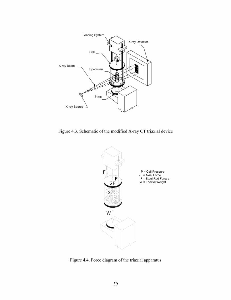
Figure 4.3. Schematic of the modified X-ray CT triaxial device.......................................39
Figure 4.4. Force diagram of the triaxial ...........................................................................39
Figure 4.5. Finite element model of the triaxial cell..........................................................41
Figure 4.6. Selected Von-Mises stress contours for the maximum design load (psi)
using an acrylic cell .........................................................................................42
Figure 4.7. Schematic drawing of triaxial manufactured by Tratwein .............................43
Figure 5.1. Determination of displacements of a 3×3×3 block in a 4×4×4 volume ..........50
Figure 5.2. NCC values at every voxel of the current image.............................................51
Figure 5.3. M-DST flowchart ............................................................................................55
Figure 5.4. Determined 3-D displacement fields for imposed displacements of 3,
3, and 5 pixels in X, Y, and Z directions, respectively (search radius is 60
pixels)...............................................................................................................57
Figure 5.5. Determined 3-D displacement fields for imposed displacements of 10, 10, and
20 pixels in X, Y, and Z directions, respectively (search radius is 20
pixels)...............................................................................................................58
xii
Figure 5.6. Determined 3-D displacement fields for imposed rotations of 5° along Z axis
using 70% similarity threshold ........................................................................59
Figure 6.1. Flowchart of the 3-D local porosity distribution computer code ....................62
Figure 6.2. 3-D local porosity distribution contours of a Silica sand specimen in XY plane
............................................................................................................................................64
Figure 6.3. 3-D local porosity distribution contours of a Silica sand specimen in YZ plane
............................................................................................................................................65
Figure 6.4. 3-D local porosity distribution contours of a Silica sand specimen in XZ plane
............................................................................................................................................66
Figure 6.5. Histogram of 3-D local porosity distribution of a specimen of Silica sand ....67
Figure 6.6. A summary of the shear band characterization procedure ..............................69
Figure A.1. Difference between (a) digital radiograph and (b) 3-D X-ray CT image of a
cylindical soil sample.......................................................................................86
Figure A.2. Difference between (a) digital radiograph and (b) X-ray CT image of a
reinforced composite specimen (middle slice) ................................................87
Figure A.3. 3-D X-ray CT image of a battery and distribution of CT numbers ................89
Figure A.4: Variation of CT numbers along the diameter of a soil sample.......................90
Figure A.5. Artifacts (straight lines and noisy circles) on a X-ray CT slice of a
battery ..............................................................................................................91
Figure A.6. A pile of 2-D reconstructed slices to generate a 3-D CT image.....................94
Figure A.7. FlashCT facility at Washington State University ...........................................96
Figure A.8. Main components of FlashCT (or any other X-ray CT system in general)....96
xiii

Figure B.1. (a) A 2-D image and a magnified pixel (b) A 3-D image and a magnified
voxel.................................................................................................................99
Figure B.2. (a) An 8-bit gray scale image (b) logical image of the same image ............101
Figure B.3. Representation of different gray shades using 8 bits for each shade ...........101
Figure B.4. Basic colors of true color images and a sample combination of basic
colors..............................................................................................................102
Figure B.5. Relation between the crop region size and the generated volume...............105 Figure B.6. A CT slice of glass beads and logical images with different thresholds “t”
(a) original image (b) t=10 (c) t=20 (d) t=30 (e) t=40 ...................................106
Figure B.7. Variation of porosity versus threshold (the red circle corresponds to the
best threshold)................................................................................................108
Figure B.8. Brightness histogram of a CT slice of glass beads ......................................109
Figure B.9. Illustration of Otsu’s method with the logical image after application of
threshold.........................................................................................................111
Figure B.10. (a) An original CT slice of silica sand (b) filtered image using unsharp
mask ...............................................................................................................113
Figure B.11. (a) An image in spatial domain (b) the same image in frequency
domain............................................................................................................115
Figure B.12. (a) CT slice of silica sand (b) filtered image after applying Gaussian
filter................................................................................................................115
Figure B.13. Image of a text ...........................................................................................116
Figure B.14. Template image (magnified)......................................................................117
xiv

Figure B.15. Correlated image........................................................................................117
Figure B.16. Locations of template in the image (white spots) ......................................118
Figure B.17. (a) Original CT slice (b) compressed image using DCT ...........................120
Figure B.18. Parallel projection of a two dimensional function f(x,y)............................120
Figure B.19. Fan beam projection of a two dimensional function f(x,y) ........................121
Figure B.20. Radon transform of a logical image at 0° ..................................................122
Figure B.21. Radon transform of a logical image at 45° ................................................123
Figure B.22. 360 parallel projections of an image in 1° increment ................................124
Figure B.23. (a) Original gray scale image (b) logical image (c) reconstructed image
using 360 projections .....................................................................................125
Figure B.24. Reconstructed image using 36 projections ................................................125
Figure B.25. Reconstructed image using 3600 projections ............................................125
Figure B.26. (a) Original image (b) image after skeletonization....................................126
Figure B.27. (a) Original image (b) image after filling holes (closed loops) .................127
Figure B.28. A gray scale image of four circles touching two by two ...........................128
Figure B.29. Representation of circles in Figure B.29 assuming an elevation of gray
shade values at each pixel ..............................................................................129
Figure B.30. (a) A logical CT image of glass beads (b) watershed transform of the image
(c) segmented image ......................................................................................130
Figure B.31. Correction of oversegmentation problem in Figure B.31(c) using minima
imposition technique......................................................................................131
Figure C.1. Another triaxial design for large load applications.......................................133
xv

LIST OF TABLES
Table 3.1. Properties of the sand and glass beads specimens ............................................19
Table 3.2. X-ray CT Scanning parameters of the specimens.............................................19
Table 3.3. REV radius and relative errors..........................................................................33
xvi

To My Wife, Morvarid
xvii

Chapter 1
INTRODUCTION
1.1 Introduction
The macroscopic stress strain response of granular materials is influenced by its
microstructure. However, the difficulties associated with internal measurements have
resulted in the development of constitutive models for granular materials mostly based on
deformations measured on the boundaries of laboratory specimens or field tests. Since
deformation is progressive, such boundary measurements may not reflect the internal
changes that occur in granular microstructure that control the overall macroscopic
response. This becomes even more complicated when the boundary condition of the
continuum is kept unchanged and the internal strains concentrate into a narrow zone
called shear band. Microscopic observations have shown several shear bands to form
initially that coalesce into one or two dominant shear bands before failure. From a
continuum mechanics standpoint, the shear band phenomenon results in a discontinuity
and classical theories fail. Therefore, shear band characteristics must be accounted for
when predicting the constitutive behavior granular materials. This is done in a
phenomenological manner by either increasing the kinematic degrees of freedom of the
particles (Vardoulakis 1989; de Borst 1992; Fleck and Hutchinson 1993) or by using
integral (Bazant and Gambarova 1984) or gradient theories (Mindlin 1964; Aifantis 1987;
Zbib and Aifantis 1988; Vardoulakis 1996; Al Hattamleh et al. 2003).
1

The fundamental continuum hypothesis is that the behavior of many physical
elements is essentially the same as if they were perfectly continuous. Physical quantities,
such as mass and density, associated with individual elements contained within a
representative elementary volume (REV) are regarded as being spread over the volume
instead of being concentrated on each particle or element. Macroscopic variables are
defined typically as averages of microscopic variables over a REV.
The REV of a continuum has been qualitatively assumed to be sufficiently large
so that granular fluctuations are smoothened out but sufficiently small so that the
macroscopic changes do not affect the result (Bear 1972; Dullien 1979). The difficulties
associated with the measurement and the characterization of granular microstructure had
prevented the identification of the size of REV in real media. Some measurements
relating to the REV of glass beads have been made recently by Culligan et al. (2004)
using a cubical elementary volume. Numerical simulations of particle assemblies have
also been made to determine the REV for relevant properties (Stroeven et al. 2004;
Ostoja-Starzewski 2005).
In the absence of experimental measurements, the minimum dimensions of the
REV are set by the grain size with the best guess being the REV is between 100 to 1000
grain diameters. For sandy soils, a REV with a radius of 10 to 20 grain diameters appears
to have been adequate for obtaining well defined average for applications in ground water
flow (Charbeaneau 2000). Despite all the hurdles, the notion of REV is absolutely
essential for engineering applications because it enables the use of continuum measures
that can be adopted in practice. This study makes use of the current advances in
microstructure characterization to accurately quantify the characteristics of REV of sands
2

and glass beads nondestructively using high resolution X-ray computed tomography
(X-ray CT).
Few studies have been performed to monitor granular deformation using X-ray
CT in real time. Geraud et al. (1998) have used CT to observe crack locations in granitic
samples subjected to heat, low confining pressure and axial loading. A real time X-ray
CT triaxial testing was performed on a coal specimen to determine the
meso-damage evolution law (Ge et al. 1999). Similar X-ray CT triaxial tests have been
performed on soils to study evolution of shear bands in a qualitative manner (Otani et al.
2000 and 2001). By tracing the movement of glass beads within a hot mix asphalt
triaxial specimen Chang et al. (2003) have made quantitative measurements of the
displacement field as well as the changes in the fabric tensor. Sun et al. (2004) have
performed a series of triaxial tests on a silty clay soil using a medical CT scanner and
related the CT numbers to stress-strain behavior of the soil. These measurements were
limited to the determination of damage and heterogeneity of the intact clay. Desrues et al.
(1996) studies local void ratio in the localization zones in triaxial tests on sand using
X-ray CT. Desrues (2004) studied evolution of shear band in triaxial specimens in an
aluminum cell. However, the tests were not performed directly inside the scanner
measuring field.
None of the above studies have quantified the displacements of the soil particles
and evolution of shear band characteristics nondestructively. In this study, a special
triaxial apparatus is designed to perform real time monitoring of deformation within the
X-ray CT chamber. The displacement field is calculated by processing of the X-ray CT
3

images in 3-D using special computer vision techniques. The local void ratio changes at
various strain levels are monitored to study the evolution of shear bands.
1.2 Objectives
The main objectives of this research are to:
1. Study the characteristics of the representative elementary volume using
X-ray CT.
2. Develop a novel triaxial apparatus for use with X-ray CT for real time
monitoring of granular microstructure evolution.
3. Develop a method to determine the 3-D internal displacement field and local
porosity distribution using X-ray CT images.
1.3 Organization of the Thesis
A background to this study is given in chapter 2. It includes past studies on real
time monitoring of shear band evolution and characterization. The results, conclusions,
advantages and drawbacks of these studies are discussed briefly. The chapter also
includes discussion on methods to determine 2-D displacement fields within soil
specimens and three dimensional fields for asphalt specimens.
Representative elementary volume (REV) of sand is discussed in chapter 3. REV
and its characteristics for glass beads, silica sand, and Ottawa sand are studied. An
interactive 3-D image processing computer program is developed. The effects of the
location of the REV center, shape and angularity of particles on the size of REV are
studied.
4

The development of a novel triaxial device that can be placed inside the X-ray CT
chamber is detailed in chapter 4.
Chapter 5 describes the extension of 2-D computer vision techniques to 3-D to
trace displacement fields. The algorithm of the developed interactive computer program,
based on template matching technique is provided. Verification of the program is
examined by moving several 3-D images with known displacements.
Development a method to characterize 3-D porosity distribution is explained in
chapter 6. Variation of the local porosity is applied as a criterion to study the evolution of
shear band. A series of computer programs are developed to accomplish these tasks.
Chapter 7 includes a summary of the conclusions, and findings of the study, as
well as recommendations for future research on this topic.
Basic details on X-Ray Computed Tomography, an overview to digital image
processing, and an alternate design of X-ray CT triaxial for large loads are given in
Appendices A, B, and C. User’s manuals of the various computer programs such as
MFC, M-REV, and M-DST computer programs are provided in an internal report of
Washington State University (Razavi 2006).
5

Chapter 2
BACKGROUND
2.1 Introduction
X-ray computed tomography (CT) is an advanced imaging technique, which
generates 3-D high resolution images (down to 5 µm spatial resolution at the present
time) of the microstructure of engineering materials. This resolution is sufficient to
detect and separate sand particles. X-ray CT combined with testing instruments and
image processing techniques enable us with a capability to advance the state-of-art in
microstructure characterization and monitoring of the desired variables in real time.
The development of a triaxial X-ray cell in the early 90’s (Geraud 1991; Vinegar
et al. 1991) was a significant step in studies associated with real time monitoring of
geomaterials using X-ray CT. Since then the number of studies in this area have been
growing significantly with improving capabilities of the X-ray CT machines, computer
hardware and software, and image processing techniques.
2.2 Determination of Representative Elementary Volume using X-ray CT
X-ray CT has been used to measure different properties of porous media such as
volume fractions, porosity, and pore size distribution (Warner et al. 1989; Spanne et al.
1994; Auzerais et al. 1996; Klobes et al. 1997; Clausuitzer and Hopmans 1999; Cislerova
and Votrubova 2002; Al Ramahi 2004; Al Raoush and Willson 2005; Al Raoush and
Alshibli 2006). Three different regions in the plot of porosity versus the size of a cubical
6

elementary volume for glass beads specimens were recognized by Culligan et al. (2004).
These regions are microscopic fluctuations, constant region, and macroscopic
heterogeneity, which had been introduced by Bear (1972) and Dullien (1979).
Measurement of REV for sand based on pore network properties from 3-D X-ray CT
images also appears in the works by Al Roush and Willson (2005). All the past studies
suffer from using glass beads instead of real sand or using a cubical region instead of a
spherical region or both.
2.3 Triaxial and X-ray CT for Real Time Monitoring
X-ray CT has been used widely to characterize soil microstructure and evolution
of shear band (Desrues et al. 1996; Tani 1997; Shi et al. 1999; Otani 2000; Alshibli et al.
2000, 2003; Wang 2004; Viggiani 2004; Desrues 2004).
The regular method to hold the locations of grains is to use of a low density
adhesive material like resin filling the pore spaces (Alshibli et al. 2000). However, a
fixed specimen with resin can no longer be used for the next loading or unloading step.
This poses problems in the study of any strain dependent phenomena, such as evolution
of shear band in a particular specimen. In addition a small disturbance due to injection of
resin into the pores is always expected. To overcome these difficulties a few researchers
modified the triaxial apparatus to load the specimen and take CT images at the same time.
However, it is important to keep in mind that at the present time even the fastest CT
scanners need a couple of minutes (depends on the image size and quality) to take a 3-D
CT image, and on the other hand the specimen cannot be loaded during scanning to avoid
blurriness.
7

Geraud et al. (1998) have used X-ray CT to observe crack locations in triaxial
granite samples subjected to heat up to 180°C and a maximum confining pressure of
10 MPa. They developed a triaxial X-ray transparent cell for real time monitoring
(Geraud 1991; Vinegar et al. 1991). The cell had to withstand a maximum confining
pressure of 28 MPa and temperature of up to 180° C for granite samples 40 mm in
diameter. They used a beryllium tube to use as for the confining pressure cell and an
aluminum tube to compensate the strain induced by the confining pressure. In this
manner they could observe the porosity variations under different mechanical and
thermal loading conditions directly.
Ge et al. (1999) used the triaxial apparatus in X-ray CT to find a meso-damage
evolution law for coal in real time. Li and Zhang (2000) monitored the changes in the
structure of road foundation soil in uniaxial compression test with X-ray CT.
Otani et al. (2001) developed a new triaxial apparatus for maximum axial load
and confining pressure of 1 kN and 400 kPa, respectively. The steel rods around a
transparent cell were removed to enable X-ray penetration. A motor was placed on top of
the cell to apply loads. The size of soil specimen was limited to 50 mm in diameter and
100 mm in height. Triaxial compression tests under consolidated drained conditions
were conducted on Toyoura Sand with relative density of 65.3% (minimum dry density
of 1330 kg/m3 and maximum dry density of 1650 kg/m3). The specimen was
consolidated to 49 kPa confining pressure. It was scanned before applying the axial load
to have an image of the initial condition. Loading and unloading of the specimen was
performed at strain level intervals of 3%. The specimen was scanned when the deviatoric
stress reached zero to avoid the effect of stress relaxation (Otani et al. 2001). This
8

process was continued until a strain level of 15.0%. The X-ray CT system needed 5 min
to scan one slice of CT images. Based on a qualitative analysis, the shape and
characteristics of the soil failure were evaluated.
Damage evolution of natural expansive soil during triaxial test was studied by Lu
et al. (2002) using X-ray CT. Viggiani et al. (2004) used a compact triaxial apparatus
similar to that of Otani et al. (2001) to conduct a qualitative study on localized
deformation in saturated Beaucaire Marl (a sedimentary soil) using X-ray CT.
Sun et al. (2004) studied deformation characteristics of triaxial silty clay
specimens using a medical X-ray CT scanner. Inhomogeneity and original damage of the
silty clay were observed by inspection of the CT images and variation of CT numbers.
The triaxial apparatus was placed horizontally inside the medical X-ray CT scanner.
Therefore, the tests cannot be considered to be axisymmetric.
2.4 Internal Displacement Fields using X-ray and X-Ray CT
There are two different techniques to calculate the internal displacement fields
using X-ray or X-ray CT at the present time; tracing easily X-ray detectable markers such
as small metallic spheres (Nemat-Nasser and Okada 2001; Wood 2002) or wires (Alshibli
and Alramahi 2006), and numerical techniques based on computer vision description
(White and Bolton 2001).
Zhou et al. (1995) developed a constrained nonlinear regression model for
estimation of displacement fields from a sequence of 3-D X-ray CT images for small
displacement gradients. It was shown that the method can determine displacement fields
over a range of inter-image displacements of up to eight pixels accurately. Quantitative
measurements of displacement fields as well as changes in fabric tensor within hot mix
9

asphalt and glass bead specimens were made by Chang et al. (2003). By tracing the
movement of glass beads in X-ray CT images, the analysis consisted of a 3-D cubic grid
embedded in the domain. Neighboring grains are identified within an examination
distance. The choice of the distance is depends on the heterogeneous deformation scale.
A linear displacement field based on the least square method is lead to fit the
displacements of the 18-26 neighboring grains within the examination distance.
Cross correlation or template matching is a classic pattern recognition technique
to determine the relative displacements between two images by finding the maximum
similarity between different blocks on them. In geotechnical engineering, it has been
used to monitor soil deformations during shear (Horii et al. 1998; Guler et al. 1999;
White et al. 2001; Rechenmacher and Saab 2002; Sadek 2002). Cross correlation scheme
also has been used for monitoring fracture processes in concrete (Shah and Choi 1996;
Lawler and Shah 2002). Liu and Iskander (2004) developed an advanced algorithm for
cross correlation called adaptive cross correlation (ACC) method to reduce the errors
associated with conventional cross correlation technique. ACC technique was used to
determine the 2-D displacement fields under a strip footing by comparing images before
and after deformation.
2.5 Experimental Observations and Characterization of Shear Bands in Sands
Experimental observations on shear bands have been made by several
investigators using a biaxial loading equipment (Vardoulakis 1980; Oda et al. 1982; Han
and Drescher 1993; Yoshida et al. 1994; Pradhan 1997; Finno et al. 1997; Oda and
Kazama 1998; Alshibli and Sture 2000), simple shear apparatus (Budhu 1984), triaxial
apparatus (Desures and Hammad 1989; Yagi et al. 1997; Oda et al. 2004), torsional shear
10

apparatus (Schanz et al. 1997), and true triaxial apparatus (Wang and Lade 2001). Figure
2.1 shows X-ray CT images around shear band formed in a sand triaxial specimen (Oda
et al. 2004).
Figure 2.1. 2-D X-ray attenuation images around a shear band (Oda et al. 2004):
(a) 2-D image of x1-x3 plane (b) 2-D image of x1-x3´ plane inside
(b) the shear zone (c) 2-D image of x1´-x2 plane
Several different techniques have been used to characterize the shear bands in
sand including video images (Saada et al. 1999), digital imaging (Alshibli et al. 1999;
11

Gudehus and Nubel 2004), radiography (Nemat-Nasser and Okada 2001), X-ray CT
(Alshibli et al. 2000; Desures et al. 1996; Tani 1997; Otani 2001; Desures 2004), high
speed cameras (Saada et al. 1994), and stereophotogrammetry (Finno et al. 1996). The
main focuses of these studies are on shear band inclination, thickness of shear band, and
inception of localization.
12

Chapter 3
REPRESENTATIVE ELEMENTARY VOLUME ANALYSIS
FOR POROSITY FOR SAND
3.1 Introduction
The methods of continuum mechanics have provided an effective means of
predicting the behavior of the collection of a large number of elements. The fundamental
continuum hypothesis is that the behavior of many physical elements within a control
volume is essentially the same as if they were perfectly continuous. If the size of the
control volume is small, the behavioral property is likely to vary spatially, and the
medium is termed heterogeneous although the spatial variation may be smooth. When
progressively larger control volumes are used the value of a specific property may tend
towards a constant value everywhere in the medium. In such cases, these volumes are
defined as the representative elementary volumes and the medium is classified as
homogenous. Specifically, physical quantities such as mass and density, associated with
individual elements contained within a representative elementary volume (REV) are
regarded as being spread over the volume instead of being concentrated on each particle
or element. Macroscopic variables are defined typically as averages of microscopic
variables over a REV and represent the property of the medium regardless of location.
REV is used extensively in multiscale engineering problems and has facilitated the
development of a number of macroscopic measures for the description of the mechanistic
13

and transport behavior of particulate media (Christofferson et al. 1981; Chang 1987;
Jenkins 1987; Walton 1987; Meegoda 1997; Muhunthan et al. 1996; Masad et al. 2000).
The fundamental ideas relating to the relevance and existence of REV in granular
materials can be illustrated by following the elegant analysis of a one dimensional
continuum model by Roberts (1994). Suppose we wish to measure the density of the
collection of granular particles at some point x and at some time t placed along a
one-dimensional continuum. This can be done by using a sampling length L of the
continuum, centered at x, and measuring the mass m of this material in this interval. The
density can then be computed by (Roberts 1994):
LtxLmtxL ),;(),;( =ρ (3.1)
The density as computed from Equation 3.1 will be a function of not only of
position but also of the sampling length L as shown qualitatively in Figure 3.1. This
graph has three distinct regions: in region I, the average density ρ(L) is dominated by
microscopic molecular fluctuations caused by the influence of chance when there are
only a small number of molecules in an averaging length; in region (II), ρ(L) is
essentially constant; while in region III ρ(L) varies smoothly, the variations being caused
by the macroscopic non-uniformity of the material. The features of Figure 3.1 for
average density are characteristic of other granular properties such as porosity (Bear
1972).
Based on the features described above the REV of a continuum has been
qualitatively assumed to be sufficiently large so that granular fluctuations are smoothened
out but sufficiently small so that the macroscopic changes do not affect the result (Bear
1972; Dullien 1979). The difficulties associated with the measurement and the
14

characterization of granular microstructure had prevented the identification of the size of
REV in real media except in a few cases. Some measurements relating to the REV of
glass beads (Culligan et al. 2004) and of ooid sand (Al-Raoush and Willson 2005) have
been made recently using a cubic elementary volume. Numerical simulations of particle
assemblies have also been made to determine the REV for relevant properties (Stroeven
et al. 2004; Ostoja-Starzewski 2005).
Figure 3.1. Three different regions of variation of density versus length (Roberts 1994)
Recent advances in imaging techniques such as X-ray computed tomography and
magnetic resonance imaging have provided geotechnical researchers with superior tools
to characterize the microstructure of granular materials (Desrues et al. 1996; Alshibli et
al. 2000; Wang et al. 2004). X-ray computed tomography image analysis can be used to
15

nondestructively characterize the 3-D microstructural features of granular materials and
their evolution with shear deformation.
This study makes use of the current advances in microstructure characterization to
accurately quantify the characteristics of REV of sands and glass beads. High resolution
X-ray computed tomography is used to obtain 3-D images. These images are post
processed using robust algorithms to study the variation of the porosity within a spherical
volume element.
Based on the features described above the REV of a continuum has been
qualitatively assumed to be sufficiently large so that granular fluctuations are smoothed
out but sufficiently small so that the macroscopic changes do not affect the result (Bear
1972; Dullien 1979). The difficulties associated with the measurement and the
characterization of granular microstructure had prevented the identification of the size of
REV in real media. Some measurements relating to the REV of glass beads have been
made recently by Culligan et al. (2004) using a cubical elementary volume. Numerical
simulations of particle assemblies have also been made to determine the REV for relevant
properties (Stroeven et al. 2004; Ostoja-Starzewski 2005).
In the absence of experimental measurements, the minimum dimensions of the
REV are set by the grain size with the best guess being the REV is between 100 to 1000
grain diameters. For sandy soils, a REV with a radius of 10 to 20 grain diameters appears
to have been adequate for obtaining well defined average for applications in ground water
flow (Charbeaneau 2000). Despite all the hurdles, the notion of REV is absolutely
essential for engineering applications because it enables the use of continuum measures
that can be adopted in practice.
16

This part of the study makes use of the current advances in microstructure
characterization to accurately quantify the characteristics of REV of sands and glass
beads. High resolution X-ray CT is used to obtain 3-D images. These images are post
processed using robust algorithms, and the variation of the porosity within a spherical
volume element is studied.
3.2 Materials and Methods
Specimens were prepared from Ottawa 30-40 sand, silica 30-40 sand, and glass
beads with average particle diameters of 6 mm, and 1.6 mm. The shape of the particles
was determined by the average axial ratio, n , defined as the average ratio of the apparent
longest axis, L1, to the apparent shortest axis, L2, of particles:
i
N
i LL
Nn ∑
=
=
1 2
11 (3.2)
where N is the number of particles.
The axial ratio of each material was estimated based on measurements made on
398, 261, and 150 particles on digital photographs for silica sand, Ottawa sand, and glass
beads, respectively, using MATLAB image processing toolbox (IPT version 5.1), and
was reported in Table 3.1. It can be seen that glass beads are nearly spherical particles,
Ottawa sand is composed mainly of subrounded particles, and silica sand is composed
mainly of elongated particles. Specific gravity of these materials is also given in
Table 3.1.
Cylindrical specimens of dry silica sand and Ottawa sand with different porosities
(MR015SON to MR022SON) were prepared in the laboratory. They were compacted in
five layers by tamping on the sides of the plastic mold. Two specimens of glass beads
17

(MR023GLN and MR024GLN) were also prepared. All of the specimens were scanned
using X-Ray CT and their 3-D images obtained. Although use of higher magnification
gives an image with a better resolution, required memory to store the image increases by
the third power of magnification. For example, if a 3-D CT image of a part needs 1 GB
memory then increasing the magnification to 2 times, increases the memory usage to
8 GB. Therefore, several preliminary scans were performed to choose the optimum
magnification to attain the best resolution within the constraints of the computer memory
and the ability to process the images. Based on the results to minimize the error in
processing the images, it was found that a magnification of 3.1 was sufficient for
specimens MR015SON through MR023GLN, and a magnification of 1.8 for specimen
MR024GLN. Table 3.2 shows the X-ray CT scanning parameters, image resolution, and
number of voxels for each specimen in the study.
18
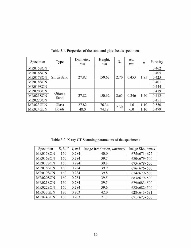
Table 3.1. Properties of the sand and glass beads specimens
Specimen Type Diameter, mm
Height, mm Gs
d50, mm n Porosity
MR015SON 0.462 MR016SON 0.405 MR017SON 0.425 MR018SON 0.401 MR019SON
Silica Sand 27.82 150.62 2.70 0.453 1.85
0.444 MR020SON 0.419 MR021SON 0.412 MR022SON
Ottawa Sand 27.82 150.62 2.65 0.246 1.40
0.451 MR023GLN 27.82 76.34 1.6 1.10 0.550 MR024GLN
Glass Beads 48.0 74.18 2.30 6.0 1.10 0.479
Table 3.2. X-ray CT Scanning parameters of the specimens
Specimen E, keV I, mA Image Resolution, µm/pixel Image Size, voxelMR015SON 160 0.284 40.0 675×671×672 MR016SON 160 0.284 39.7 680×679×500 MR017SON 160 0.284 39.8 675×678×500 MR018SON 160 0.284 39.9 676×676×500 MR019SON 160 0.284 39.8 674×679×500 MR020SON 160 0.284 39.5 683×679×500 MR021SON 160 0.284 39.5 679×683×500 MR022SON 160 0.284 39.6 682×682×500 MR023GLN 180 0.203 42.0 628×643×591 MR024GLN 180 0.203 71.3 671×673×500
19

3.3 REV and Image Characterization
An interactive computer program, M-REV, was developed in MATLAB to
perform the analyses on the 3-D CT images. The main features of the
M-REV program are presented in the form of a flowchart in Figure 3.2. First, the 3-D CT
image is read and stored as a 3-D array so that the reconstructed CT slices show the top
view of the specimen. If necessary the gray scale values of the voxels can be rescaled to
spread the histogram of the gray scale values between 0 and 255. This is called
histogram equalization for intensity adjustment. In most cases, CT slices contain some
noise on the image background which tends to propagate a significant error in processing.
User can specify the outer boundaries of the specimen in the program to remove
background noise. Figure 3.3(a) shows a two-dimensional CT slice of glass beads in
which the wall of the container and noise in the background are evident. Figure 3.3(b)
shows the same slice after removal of the container walls and the background noise with
intensity adjustment.
20

Fix Location of the Center of Volume Element
Segmentation
Remove Background Noise
Adjust Image Intensity
Convert Image to 8-bit Gray Scale Image
Read 3-D X-ray CT Image
Start
Ri =Ri-1+∆R
Find Porosity
Save Output Results
s
End
Plot Porosity versus Eleme Volume Radius
R ≤ Rmax
Figure 3.2. Flow chart of
21
ntary
No
Ye
the M-REV program

(a) (b)
Figure 3.3. (a) A 2-D CT slice of glass beads before any corrections (b) the same CT slice
after circular cropping, intensity adjustment, and background noise removal
In the next step, the image is converted to a logical image (black and white image
or BW image) using a threshold value. In this study, the method proposed by Otsu
(1979), which chooses the threshold to minimize the interclass variance of the black and
white pixels, was applied to find the best threshold to convert the image to a logical
image (Appendix B). The result is as shown in Figure 3.4(a). It is noted, however, that
the user can manually choose a desired threshold between 0 and 255 to separate the
features by looking at the image histogram and visual inspection. It can be seen that use
of a threshold alone does not separate the grain boundaries very well. Thus, and
advanced image processing technique called watershed transform (Gonzalez et al. 2004;
Russ 2002) with gradient is applied to segment or separate the contact points of particles.
The watershed transform applies the same idea as in geography for segmentation of the
gray scale images. Watershed ridgeline is the line, which separates the two connected
objects. In order to apply watershed transformation to binary images, first a
22

transformation of the distance from every pixel to the nearest nonzero valued pixel is
calculated. Once the distance transformation of the image is determined, then watershed
transformation is applied. The resulting watershed image will appear as shown in
Figure 3.4(b).
(a) (b)
Figure 3.4. (a) Converted gray scale image to a logical image using Otsu’s method
(b) watershed transform of the image
The watershed image is subtracted from the original image so as to give the image
in Figure 3.5(a). In some cases, even with the use of watershed transform the boundaries
of the particles may not be clear as is the case in Figure 3.5(a). For such cases,
application of a gradient prior to using the watershed transformation is recommended. In
the gradient method, the image is filtered by a 3×3 Sobel mask, which approximates
vertical or horizontal gradients of the image (Gonzalez et al. 2004). In case of over-
segmentation due to watershed transform as in Figure 3.5(a) in which many grains have
been segmented around the boundaries and inside, the method of regional minima is
23

applied to remove the unnecessary segmentation within the grains (Gonzalez et al. 2004).
Figure 3.5(b) is the result of the application of the regional minima algorithm to
Figure 3.5(a) to fix over-segmentation. Additional details of the above standard image
processing techniques are available from text books (Russ 2002; Gonzalez et al. 2004).
(a) (b)
Figure 3.5. (a) Segmentation of the image (over segmentation) (b) final segmentation
(correction of over segmentation using regional minima)
The REV program chooses a spherical volume element whose center can be fixed
anywhere within the specimen (Figure 3.6). Once the location of the center is fixed, the
radius of the sphere is increased from zero to its maximum limited by the specimen
boundary. The variation of porosity with the radius of volume element is plotted for each
incremental step of the spherical radius.
In REV program, the user can examine the images from three different
viewpoints; top, front, and right. The user can zoom (in or out) the images, find the
location of each plane, the gray scale value of any voxel, and distance between different
24

objects on images. The output results are saved in MATLAB, and can also be exported
to a spreadsheet.
Figure 3.6. A sample plot of variations of porosity versus the radius of the spherical
volume element.
25

3.4 Results and Discussion
Six different assemblages of 8 to 10 identical spheres with diameter d as
suggested by Graton et. al. (1935) are shown in Figure 3.7 along with a sphere with a
radius of twice the diameter of identical spheres. These basic assemblages can be fitted
within the middle sphere and the pattern repeated randomly to produce a homogeneous
medium. This in effect means that a basic volume element with a radius of 2 to 3 times
of sphere diameters is expected to be the REV for random packing of identical spheres.
It is also noted that inspection of the 3-D CT images of the glass beads specimens showed
that the assemblage (α) is the dominant pattern that was repeated.
Figure 3.7. Assemblages of identical spheres with diameter d around a spherical volume
element with a radius of 2d. (Note, most of the observed patterns on 3-D CT
images were similar to assemblage α)
26

Figure 3.8 shows the variation of porosity with the radius of the spherical volume
element for glass beads specimens. It can be seen that the variation attains a constant
value after an initial fluctuation. The specimens of glass beads are similar to identical
spheres with repeated packing pattern and homogenous. The plateau in region II will
continue at large radii as is evident from Figure 3.8. The normalized plot for one of the
glass beads specimen (MR023GLN) with respect to the average diameter of the beads
(d50) is shown in Figure 3.9. It is seen that the radius of the REV is between 2 and 3
times of the average spheres diameters as expected for an assemblage of random spheres.
Figure 3.8. Porosity versus volume element radius for glass bead specimens
27

Figure 3.9. Normalized REV range to d50 for small size glass beads
Figure 3.10 shows the variation of porosity versus the radius of the spherical
volume element for five silica sand specimens. It can be seen that the variation of the
porosity of all five specimens show the characteristics of regions I, II, and III in
Figure 3.1; a segment with fluctuation part at the beginning, a constant segment in the
middle and a monotonically increasing segment at the end. It is also evident that the
boundaries of the region are nearly the same in all of the specimens. The same trend is
evident in the case of Ottawa sand (Figure 3.11) although the region III in these two
materials has both an increase and a decreasing trend.
28

Figure 3.10. Porosity versus volume element radius for silica sand specimens
29

Figure 3.11. Porosity versus volume element radius for Ottawa sand specimens
30

Figure 3.12 shows the plot of variation of porosity respect to the normalized
radius of the spherical volume element for two selected specimens of silica sand
(MR018SON) and Ottawa sand (MR020SON). It can be seen that the REV radius for
Ottawa sand is formed with more grains with a diameter of d50. The ranges of
representative elementary volume radius for all specimens are summarized in Table 3.3.
Comparison those ranges with d50 of sand specimens shows that the ratio of the REV
radius to d50 is about 5 to 11 times of for silica sand, 9 to 16 times for Ottawa sand, and
about 2 to 3 times for uniform glass beads with random packing.
Figure 3.12. Normalized REV range to d50 for two selected specimens of silica sand
(MR018SON) and Ottawa sand (MR020SON)
31

Figure 3.13 shows effect of the center location of the REV element within the
specimen on the size of REV for specimen MR018SON. The location of the center of
spherical volume element was changed from point A to F with the numbers within the
brackets beside each letter indicating the coordinate. It can be seen that change in the
location of the center of spherical volume element does not have a significant effect on
REV radius. This was the case for other specimens as well.
Figure 3.13. Porosity versus volume element radius for six different center locations of
specimen MR018SON
32

The last column of Table 3.3 shows the comparison of the porosity obtained from
image processing (nip) and the laboratory measured values (nlab). The values compare
very well. It is noted, however, that the relative error is much higher in Ottawa sand.
This sand had finer grains and although the size of the finest grains of Ottawa sand
specimen was larger than the resolution of the CT image, fewer pixels are used to form
the image in sands with finer grains for a given magnification. This problem tends to
propagate the error in processing the images and results in a higher relative error.
Smaller specimens with higher magnification will reduce such error but the processing is
limited by available memory.
Table 3.3. REV radius and relative errors
Type Specimen RREV Range, mm RREV/d50 Range nip nlab % ErrorMR015SON [2.54, 3.34] [5.6, 7.4] 0.454 0.462 1.73 MR016SON [3.04, 4.66] [6.7, 10.3] 0.412 0.405 -1.73 MR017SON [2.46, 3.25] [5.4, 7.2] 0.412 0.425 3.06 MR018SON [2.54, 4.83] [5.6, 10.7] 0.401 0.401 0.00
Silica Sand
MR019SON [3.29, 4.26] [7.3, 9.4] 0.422 0.444 4.95 MR020SON [2.63, 3.80] [9.9, 15.4] 0.379 0.419 9.55 MR021SON [2.44, 3.64] [9.9, 14.8] 0.429 0.412 -4.13 Ottawa Sand MR022SON [2.23, 2.73] [9.1, 11.1] 0.435 0.451 3.55 MR023GLN [3.59, 3.70] [2.2, 2.3] 0.543 0.550 1.27 Glass Beads MR024GLN [12.03, 12.23] [2.0, 2.04] 0.485 0.479 -1.25
3.5 Discussion on REV
While the use of REV in developing macroscopic measures has been used widely
in fluid flow and continuum mechanics applications, the existence of REV and its size
has remained conjectural. It has never been identified systematically in real media in the
past. This study presents a unique technique to quantify the characteristics of
33

representative elementary volume in granular materials. It makes use of the X-ray
computed tomography imaging techniques to examine the presence of REV.
An interactive 3-D image-processing program was developed to process the 3-D
CT images and choose the REV. The effect of the shape and size of the particles,
specimen porosity, and location of the REV center were examined in this study using
different specimens of spherical glass beads, silica sand and Ottawa sand. The results
show three different characteristic regions: a microscopic fluctuation region, constant
region, and monotonically increasing/decreasing region.
The REV radius for the glass beads specimens and random packing is found to be
2 to 3 times of the identical average sphere diameter. The radius for silica sand
composed mainly of elongated particles is between 5 to 11 times of d50, and for Ottawa
sand composed mainly of subrounded particles is between 9 to 16 times of d50. These
values appear to justify the use of 10 to 20 diameters of sand grains adopted in some
studies. The fact that the radius of REV appears to decrease with elongation and
angularity leads us to believe that interlocking may be a contributor in determining its
size.
The proposed method is general and it can be applied for any granular or
perforated material if the void sizes are more than the maximum CT image resolution.
However, at the present time the maximum specimen size is limited to the capabilities of
the X-ray CT equipment and available memory to process the image.
On a final note, in view of its usefulness, the concept of REV relating to
numerical modeling and selection of specimen size for laboratory tests has been debated
recently. As discussed in the introduction, it is necessary to realize that the REV concept
34

is useful for obtaining average properties of a homogenous medium. On the other hand,
element tests on natural media inevitably encounter heterogeneity and the classical
continuum hypothesis breaks down. In this case, the size of REV becomes
scale-dependent. One may define a REV size for a specific sized specimen in a
laboratory-scale problem but this may not be applicable to larger sized specimens or
field-scale problems, where heterogeneity at several scales exists. Additional non-local
continuum measures are needed to fully describe scale effects in such heterogeneous
media (See Al Hattamleh et al. 2003).
35
Chapter 4
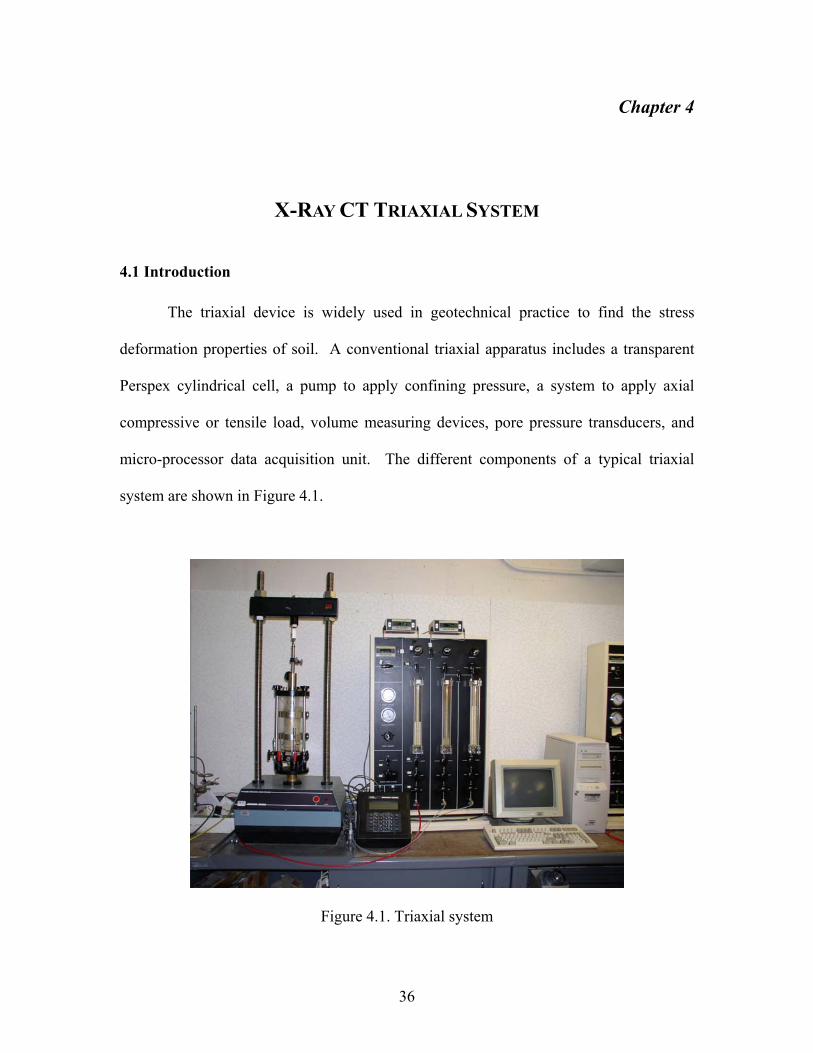
X-RAY CT TRIAXIAL SYSTEM
4.1 Introduction
The triaxial device is widely used in geotechnical practice to find the stress
deformation properties of soil. A conventional triaxial apparatus includes a transparent
Perspex cylindrical cell, a pump to apply confining pressure, a system to apply axial
compressive or tensile load, volume measuring devices, pore pressure transducers, and
micro-processor data acquisition unit. The different components of a typical triaxial
system are shown in Figure 4.1.
Figure 4.1. Triaxial system
36

However, use of the conventional triaxial system, especially the cell and loading
arrangement inside the X-ray CT chamber is impractical. Thus, a new design is needed
to enable simultaneous measurements of microstructure changes with shearing. The
design of a new triaxial apparatus for use with the X-ray CT system at Washington State
University is presented in this chapter.
4.2 Characterization of the Soil Microstructure using Triaxial Apparatus
The soil specimen must be simultaneously scanned using X-ray CT while it is
subjected to shearing in order to develop 3-D images of soil microstructure and its
evolution. This process suffers from the following limitations.
1. There is only limited place available within the X-ray CT shield cabinet. This is
not sufficient to place a triaxial device. Furthermore, the diameter of the object
placed on the rotary stage of X-ray CT system at WSU is limited to a maximum
of 50 cm.
2. Steel rods around a conventional cell prevent X-ray from penetrating into the
specimen. This would result in CT images of the specimen that are defective for
processing. The CT image of a soil specimen obtained using a conventional
triaxial cell is as shown in Figure 4.2. It is evident that the image is not good for
processing.
3. The total weight on X-ray CT system at WSU rotary stage is limited to 500 N.
Therefore, in order to perform real time monitoring of microstructure, a new
triaxial system was designed to meet the above limitations. Such design is much
dependent on the specifications of X-ray CT system, load limitations, and cost.
37

Specimen
d
Figure 4.2. A CT slice of a soil specim
the specimen image are no
4.3 Development of a Novel X-Ray CT Tria
The past few years have seen signif
X-ray transparent materials such as glass
strength as much as twice that of grade 50 s
plastic also is a good material that resists ho
small but powerful loading systems enable u
of steel rods using GRP.
The loading frame of conventional tria
jack attached with tension bars on top of th
compressive force by the jack is counter bala
tension bars (Figure 4.4). Further, the int
external force; thus, the only applied force o
apparatus.
38
Steel Ro
Cell
en in a conventional triaxial cell (Details of
t clear.)
xial Apparatus
icant advances in developing high strength
reinforced plastic (GRP) that has tensile
teel (Dagher et al. 1997). Glass reinforced
op stress. This coupled with the advent of
s to design a triaxial cell that avoids the use
xial system is replaced with a small loading
e cell (Figure 4.3). This way, the applied
nced by the tensile forces developed in the
ernal cell pressure does not generate any
n the CT stage is the weight of the triaxial
Loading System
X-ray Detector
Cell
X-ray Beam Specimen
Stage
X-ray Source
Figure 4.3. Schematic of the modified X-ray CT triaxial device
F
2FF
W
P
P = Cell Pressure 2F = Axial Force F = Steel Rod Forces W = Triaxial Weight
Figure 4.4. Force diagram of the triaxial apparatus
39

It is noted that Otani et al. (2001) have developed a similar triaxial device for use
use with their X-ray CT. However, its capability is limited to specimen size, axial load,
and cell pressure less than 50 mm × 100 mm, 1 kN, 400 kPa, respectively.
4.3.1 Design Requirements
The design requirements for the new system are as follows:
I. Maximum enclosure box dimensions: 50 cm ×50 cm at base and 100 cm in height
II. Maximum axial load: 10 kN
III. Maximum cell pressure: 400 kPa
IV. Maximum specimen size: 150 mm × 170 mm
V. Total weight: 500 N
VI. Computer control loading system and data acquisition
VII. Total cost: less than $30,000
4.3.2 Design Feasibility Based on Finite Element Analysis
An analysis of the triaxial device was performed using a general finite element
analysis program (NISA1-II) followed by a series of extensive stress-strain analyses to
ensure the feasibility of the design. Acrylic cell, aluminum base, soil specimen,
aluminum load cap, and aluminum top end plate were modeled using 8 node solid
elements. Applied loads constituted of the weight of the system, internal pressure, axial
load on the specimen, and reactions of the tie rods on top of the cell. Zero vertical
displacement boundary conditions were applied to the nodes along the very bottom
1 NISA: Numerical Integrated Systems Analysis of elements (A family of general and special purpose finite element modeling and analysis programs for PCs, workstations, and supercomputers by Engineering Mechanics Research Corporation, Troy, Michigan)
40

nodes. A series of linear elastic analysis for the maximum design axial load (10 kN) and
maximum internal pressure (400 kPa) were performed to investigate design feasibility
and then to obtain the cell thickness. Figure 4.5 shows the finite element model of the
cell. The corresponding von-Mises stress contours on the cell for the applied load
conditions are shown in Figure 4.6. It is evident that the von-Mises stress values within
the acrylic cell are less than 10 MPa (1.5 ksi) and it is even much less than acrylic tensile
strength of 47-79 MPa. Note that though stress values are low, small elastic modulus of
the acrylic (2 GPa) tends to have large strains, which does not allow increasing the load
or cell pressure more than the design requirement values in this study. Based on the
finite analysis, it was found that such that design is feasible and a wall thickness of 5 cm
is sufficient for the cell to resist against the combined biaxial stresses. For cases
involving higher loads, a new system is needed. Details of such a system are provided in
Appendix C.
3-D 8 node solid elements
Figure 4.5. Finite element model of the triaxial cell
41

Figure 4.6. Selected Von-Mises stress contours for the maximum design load (psi)
using an acrylic cell
Modified axial deformation is calculated by subtraction elongation of the cell and
cell piston displacement. Using GRP materials instead of acrylic for the cell, allow
increasing axial load and internal pressure dramatically.
4.3.3 X-ray CT Triaxial Components
A very small electronic loading jack, called GeoJac, provides an axial load up to
10 kN. Cell pressure is generated by an air compressor, and is regulated to the desired
level using a component called DigiFlow. Both loading and data acquisition are
controlled by a computer to minimize the human error. Figure 4.7 shows different
components of the triaxial system that is under development by Trautwein Geotechnical
Testing Instruments Company based in Houston, Texas.
42
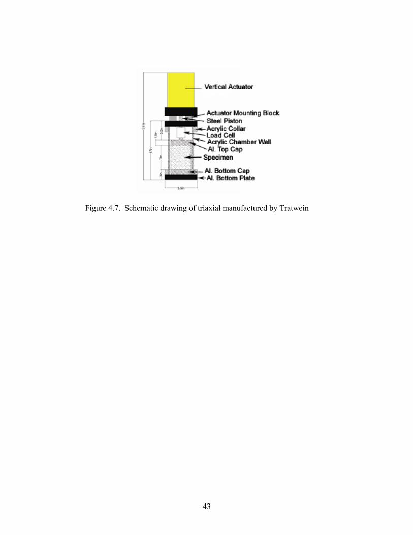
Figure 4.7. Schematic drawing of triaxial manufactured by Tratwein
43

Chapter 5
DETERMINATION OF 3-D INTERNAL DISPLACEMENT FIELDS
5.1 Introduction
Shear bands in granular materials are generally formed along three dimensional
surfaces. Detection of the shape of such these surfaces, and internal displacement fields
especially in the neighborhood of shear bands is important to characterize its features.
Shape of the shear bands may be observed and photographed directly for simple cases
such as plane strain problems. Use of small colored particles aids in the detection of the
shape of shear bands easier, though some disturbance and a change in material properties
is expected. X-ray CT can provide a 3-D image of the specimen and as such it is useful
to detect shear band characteristics, nondestructively.
Use of easily detectable material as markers, such as colored sand or tiny metallic
spheres is commonly used to find internal displacements. Colored sand layers are usually
used behind a transparent sheet and the movement of the colored particles is traced from
photographs that are taken continuously as the specimen is loaded. On the other hand,
instead of markers, a rectangular grid, made of horizontal and vertical lines, is plotted on
the transparent sheet and the displacements of the grains are obtained by tracing the
relative movement of the particles respect to the grid lines (White and Bolton 2004).
Particle image velocimetry (PIV), which is a technique to find instantaneous 3-D velocity
vector in a flow field, is applied to obtain the displacements. This technique has been
shown to predict displacement fields for large scale tests with a negligible error.
44
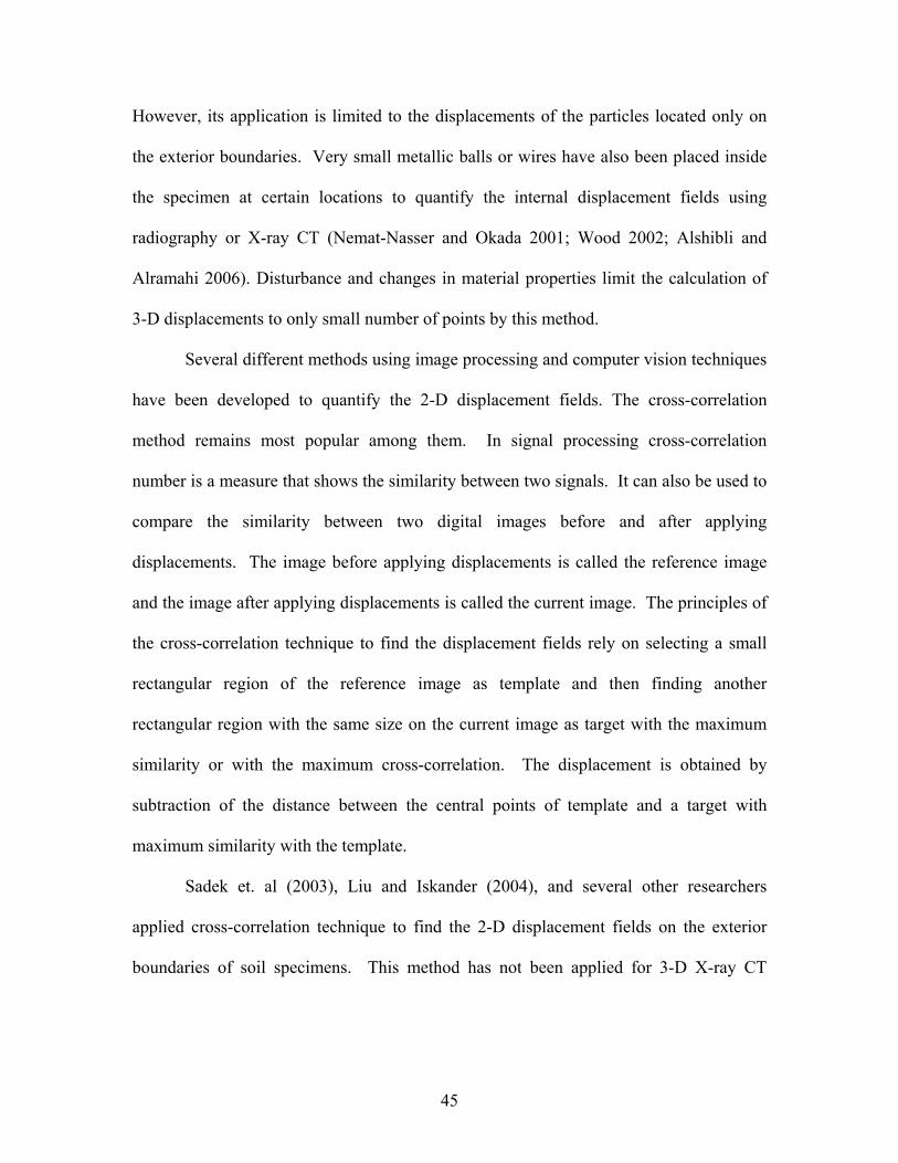
However, its application is limited to the displacements of the particles located only on
the exterior boundaries. Very small metallic balls or wires have also been placed inside
the specimen at certain locations to quantify the internal displacement fields using
radiography or X-ray CT (Nemat-Nasser and Okada 2001; Wood 2002; Alshibli and
Alramahi 2006). Disturbance and changes in material properties limit the calculation of
3-D displacements to only small number of points by this method.
Several different methods using image processing and computer vision techniques
have been developed to quantify the 2-D displacement fields. The cross-correlation
method remains most popular among them. In signal processing cross-correlation
number is a measure that shows the similarity between two signals. It can also be used to
compare the similarity between two digital images before and after applying
displacements. The image before applying displacements is called the reference image
and the image after applying displacements is called the current image. The principles of
the cross-correlation technique to find the displacement fields rely on selecting a small
rectangular region of the reference image as template and then finding another
rectangular region with the same size on the current image as target with the maximum
similarity or with the maximum cross-correlation. The displacement is obtained by
subtraction of the distance between the central points of template and a target with
maximum similarity with the template.
Sadek et. al (2003), Liu and Iskander (2004), and several other researchers
applied cross-correlation technique to find the 2-D displacement fields on the exterior
boundaries of soil specimens. This method has not been applied for 3-D X-ray CT
45

images due to some difficulties such as fluctuations of X-ray intensity with time, large
sizes of 3-D images, and extremely long processing time.
In this chapter the cross-correlation technique is extended to three dimensions and
practical methods are developed to obtain 3-D displacement fields from successive 3-D
X-ray CT images. An interactive computer program (M-DST) is developed to determine
the 3-D displacement fields using those techniques.
5.2 Cross-Correlation Technique for Pure Displacements
Any X-ray CT image can be represented by a discrete function F(Xi), which maps
point Xi(xi,yi,zi) in 3-D Euclidean space to F(Xi) or image intensity at point Xi. To
determine the internal displacement fields between two successive X-ray CT images, at
times t, and t+∆t, the image at time t is considered as template or reference image, F(Xi)
and the image at time t+∆t is considered as target or current image G(Xi). A small box
shape subvolume is taken from the current image F(Xi), which is represented by f(Xi). It
is assumed that after applying a displacement di (with three components ui, vi, wi in x, y,
and z directions, respectively) to f(Xi) there is another box shape subvolume with the
same size of the template in the current image like target g(Xi), which is the same as f(Xi),
i.e.,
)()( iii dXfXg −= (5.1)
However, in practice finding a target exactly the same as the template is nearly
impossible due to several issues such as the fluctuation of X-ray with time, particle
rotation, and noise. Therefore, Equation 5.1 is modified by an additional term to
compensate for these issues. This additional term is usually added to the template as a
remainder like η(Xi):
46
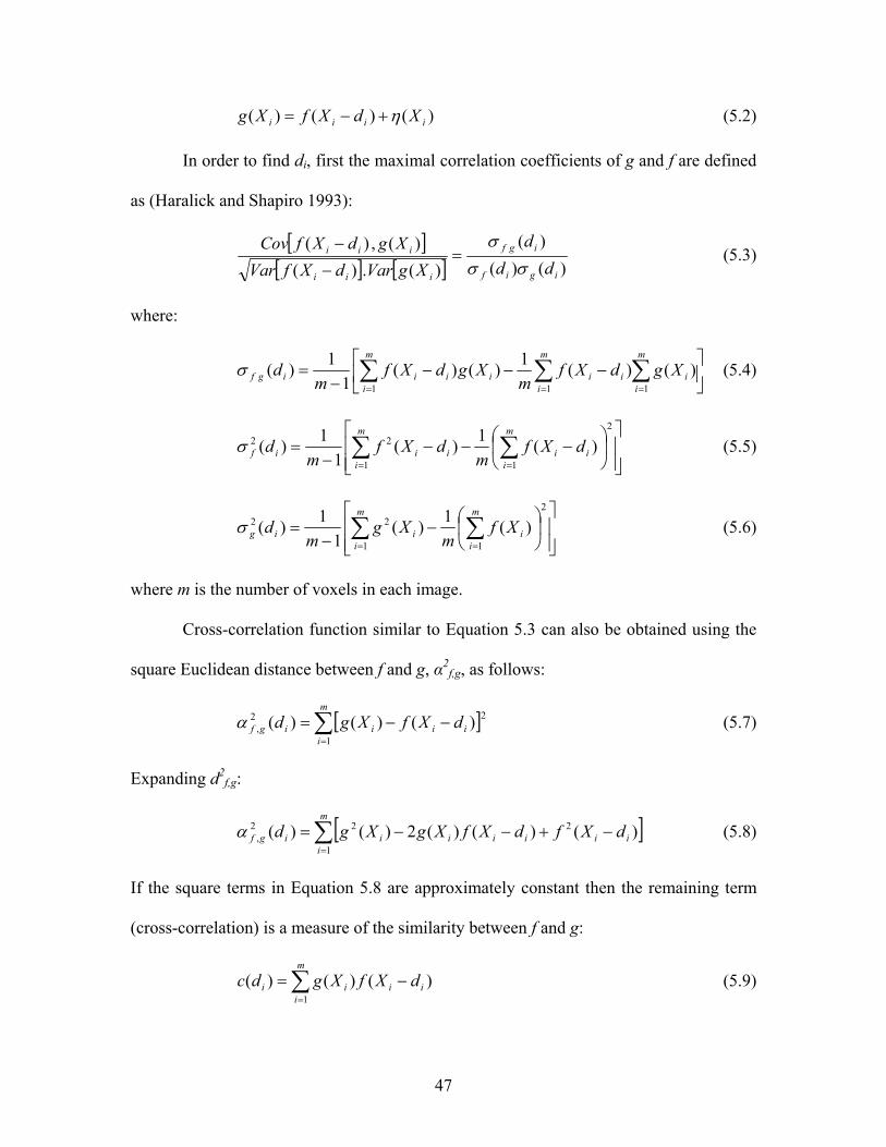
)()()( iiii XdXfXg η+−= (5.2)
In order to find di, first the maximal correlation coefficients of g and f are defined
as (Haralick and Shapiro 1993):
[ ][ ] [ ] )()(
)(
)(.)()(,)(
igif
igf
iii
iii
ddd
XgVardXfVarXgdXfCov
σσσ
=−
− (5.3)
where:
−−−
−= ∑ ∑
= =
m
i
m
i
m
iiiiiiiigf XgdXf
mXgdXf
md
1 1)()(1)()(
11)(σ ∑
=1 (5.4)
−−−
−= ∑ ∑
= =
m
i
m
iiiiiif dXf
mdXf
md
1
2
1
22 )(1)(1
1)(σ (5.5)
−
−= ∑ ∑
= =
m
i
m
iiiig Xf
mXg
md
1
2
1
22 )(1)(1
1)(σ (5.6)
where m is the number of voxels in each image.
Cross-correlation function similar to Equation 5.3 can also be obtained using the
square Euclidean distance between f and g, α2f,g, as follows:
[∑=
−−=m
iiiiigf dXfXgd
1
22, )()()(α ] (5.7)
Expanding d2f,g:
[ ]∑=
−+−−=m
iiiiiiiigf dXfdXfXgXgd
1
222, )()()(2)()(α (5.8)
If the square terms in Equation 5.8 are approximately constant then the remaining term
(cross-correlation) is a measure of the similarity between f and g:
∑=
−=m
iiiii dXfXgdc
1)()()( (5.9)
47

where c(di) is cross-correlation coefficient as a function of displacement.
Application of above cross-correlation function to find displacements has several
disadvantages (Lewis 1995). For example:
• If (image energy) varies with position, the matching algorithm based
on Equation 5.9 fails, because the square terms in Equation 5.8 were assumed
approximately to be constant.
∑=
m
iiXg
1
2 )(
• The range of the cross-correlation function depends on the size of the template.
• Equation 5.9 is not invariant with changes in image amplitude such as those
caused by changing X-ray conditions across the image sequence.
To overcome the above problems, the cross-correlation function is normalized to unit
length (Lewis 1995):
[ ][ ]
[ ] [ ]5.0
1
2
1
2
1
)()(
)()()(
−−−
−−−=
∑∑
∑
==
=
m
iii
m
ii
ii
m
ii
i
fdXfgXg
fdXfgXgdNCC (5.10)
where:
NCC(di) = normalized cross-correlation as a function of displacement di
f = average of template f
g = average of target g
The above equation is referred to as the normalized cross-correlation function. Both
correlation coefficients from Equation 5.3, and Normalized cross-correlation function
from Equation 5.10 ranges from -1 to +1, in which +1 shows 100% similarity between
template and target or both are the same; 0 means no similarity and -1 shows 100%
48

similarity in the reverse direction. In any case, the maximum absolute value resulting
from Equation 5.3 or Equation 5.10 is always considered to compare two images. Finally,
the displacement di is calculated as follows:
d (5.11) icfcgi XX −= max
where:
maxcgX = Cartesian coordinates of the target central point so that the correlation
coefficient or cross-correlation function is maximum
icfX = Cartesian coordinates of the template central point
5.2.1 Determination of 3-D Displacement Fields
The reference image is divided to small box shape subvolumes to find the
displacement fields using cross-correlation techniques. The size of the subvolumes
depends on many different factors such as image size, available computer memory, and
accuracy. Then for each template f in the reference image F a target g in the current
image G is searched so that the correlation coefficient (Equation 5.3) or normalized
cross-correlation (Equation 5.10) is maximal. The displacement di is determined based
on the maximum similarity between two blocks using Equation 5.10. In case of
significant rotations different orientations of the target must be examined to include the
effect of affine deformation (displacement and rotation). This is done by using
optimization techniques or robust statistical methods (Clocksin et al. 2002). However,
for small rotations, rotation of the target blocks may be neglected to reduce processing
time.
49

In order to illustrate the application of this technique, the displacements of a
3×3×3 block (template) in a 4×4×4 volume (reference) for a movement of 1 unit in X, Y,
and Z directions are determined. Figure 5.1 shows the reference image left and the
current image on the right. The numbers in each voxel show the image intensity at that
point. The 3×3×3 template block in the lower left corner in the template has been moved
to the upper back right corner in the current image.
147
258
369
54 687 9
21 3
98754
3216
64 51 2 3
7 8 9
12
34
1
2
3
4
63
94 51 2
7 847
1
1
96
852 3
54 6
2
321
3
987
12
34
4
Reference Image Current Image
12
34
21
43
x
yz
Template
Target
Template Center(2,2,2)
Target Center(3,3,3)
Displacement Vector(1,1,1)
Figure 5.1. Determination of displacements of a 3×3×3 block in a 4×4×4 volume
Normalized cross correlation (NCC) values for the template and all possible
targets are calculated using either Equation 5.3 or Equation 5.10. Each time the moving
block center is located at a voxel of the target to examine all voxels in the target, which
50

are 64 in this example. Elements of the moving block, which are placed outside the
target, are filled with zeros (zero padding) and maximum of the absolute values of NCC
is found. Figure 5.2 shows the plot of NCC values at every voxel of the target. This plot
has a maximum of 1 at element (voxel) number 42 corresponding to a point with
Cartesian coordinates of (3,3,3). Cartesian coordinates of the selected block in the
template is (2,2,2) and the displacements are obtained by subtracting those block center
coordinates using Equation 5.11, which are 1, 1, and 1 in X, Y, and Z directions,
respectively.
Figure 5.2. NCC values at every voxel of the current image
51

5.2.2 NCC Issues and Solutions
There are several issues with NCC that need to be resolved before programming
the method:
1. X-ray intensity fluctuates, whereas the main assumption in NCC is to use the
same X-ray intensity for both reference and current images.
2. NCC is not invariant and for the repeating patterns and affine deformation the
results may fail or incur large errors.
3. As shown in the last example, for every block in the template all the voxels in
the target must be examined. Thus NCC technique is extremely time
consuming. For a M×N×P voxel reference image and a Q×R×S voxel current
image, NCC is calculated M×N×P×Q×R×S times. For instance for a
300×300×500 voxel reference image and the same current image size, NCC
is calculated 2.025×10¹⁵ times to find the displacement at every voxel.
Besides, several times this number is needed for the total suite of operations.
It means that several months are needed to process this single problem on
personal computers with the fastest CPU at the present time (about 4 GHz).
The following solutions are provided as the solutions to overcome the issues:
1. Use of the average of several different frames (X-ray snap shots) for each
single digital radiograph and increasing the number of averaged frames
smoothes the X-ray intensity fluctuation so that it can be assumed constant
intensity with a good accuracy.
52

2. Displacements on soil specimens can be applied in small steps. When a fixed
axis test such as triaxial is used the rotation of the blocks are small as well.
Sand particles are irregular in shape, which means that no repeating pattern is
expected for an image with sufficient resolution to separate the particles.
3. When there is no information about displacements all the voxels in the current
image should be searched. Displacements of the blocks may be estimated
based on the external radial and axial displacements. Therefore, to reduce the
processing time a subvolume around a particular block from target is extracted
to search for the maximum NCC within that small subvolume. Use of fast
NCC algorithms by expanding both numerator and denominator of Equation
5.3 or Equation 5.10 (Lewis 1995; Eaton 2005), reduces the processing 20
times and even more. Finally, use of parallel processing is recommended to
further reduce the processing time.
5.3 An Interactive Computer Code to Find 3-D Displacement Fields
An interactive computer code (M-DST) was developed to find the displacement
fields by comparing template and target images using NCC technique in MATLAB
environment. Figure 5.3 shows M-DST flowchart. M-DST can load 3-D X-ray CT
images from different sources; from output of the visualization program (FlashCT-VIZ),
from horizontal X-ray CT slices, and from a 3-D array stored as a MAT files. The
program takes advantage of successive data write and read on the hard disk drive to
process large volumes. In this way only the necessary portion of the image is loaded from
hard disk drive to the random access memory (RAM). After completing the operations,
the results are saved on the hard disk drive and deleted from RAM to provide sufficient
53

free space for the next image portion. The user can extract a subvolume from the
reference image to limit the calculations to certain voxels. Displacement fields may be
determined using three different methods; fast NCC using running sum, direct
determination of NCC, and spatial correlation (inverse Fourier transform of the product
of the transform of one function times the conjugate of the transform of the other). To
ensure that the similar blocks are selected, the displacements between the blocks take in
to account only when the maximum value of NCC is more than a similarity threshold. A
similarity threshold about 95% gives acceptable results for most applications.
54

Start
Load Reference and Current Images
Input Parameters
Taking a Template block from the Reference Image
Choose a Subvolume based on the Template and Search Radius
Find NCCmax using Equation 5.3 or Equation 5.10
Yes |NCC|max < Similarity
No
Find Displacement Vector using Equation 5.11
Yes Any Unselected Block in the Reference Left?
No
Graphical and Numerical Output
End
Figure 5.3. M-DST flowchart
It is recommended to reduce this number to 70% in case of significant rotations,
unless rotation is included using optimization. However, reduction of the similarity
threshold means reduction of accuracy but less processing time.
55

5.3.1 Verification of the Computer Code
Different tests were used to verify the computer code. In the first, the current
image is generated by applying known displacements to the reference image. Then the
displacements of the reference image are determined by the program and the results are
compared. Figure 5.4 shows the displacement fields of a 3-D X-ray CT image after a
translation of 3, 3, and 5 pixels in X, Y, and Z directions (The volume size is
337×337×246 voxels and the total processing time on a 3.2 GHz Pentium IV machine is
about 17 hours. In this particular problem template size is 35×35×35 voxels, search
radius is 60 pixels and the displacements are determined for 20 voxels intervals with
100% similarity threshold). The results of M-DST are exactly the same as imposed
displacements. To check the program for larger displacements, the 3-D X-ray CT image
is translated 10, 10, and 20 pixels in X, Y, and Z directions, respectively. The results are
shown the Figure 5.5, which are identical to the imposed displacements. (To reduce the
processing time, the search radius is reduced to 25 pixels and the displacements are
determined for 35 voxels intervals. The other parameters in the program are kept
unchanged. These changes reduce the processing time significantly to 00:48:38 hours
using the same machine.)
In case of rotation of template blocks, M-DST determines rotation pattern
correctly, but there is a significant error in displacement values. For instance the results
of the 3-D X-ray CT image for a rotation of 5° (counter clockwise) around Z axis for
70% similarity threshold are shown in Figure 5.6. In this case M-DST could not find any
template and target blocks to have a similarity more than 95%. It means that for
56

significant rotations considerable error is expected, though pattern of the displacement
fields seems to be valid.
Figure 5.4. Determined 3-D displacement fields for imposed displacements of 3,
3, and 5 pixels in X, Y, and Z directions, respectively (search radius
is 60 pixels)
57

Figure 5.5. Determined 3-D displacement fields for imposed displacements of 10, 10, and
20 pixels in X, Y, and Z directions, respectively (search radius is 20 pixels)
58

Figure 5.6. Determined 3-D displacement fields for imposed rotations of 5° along Z axis
using 70% similarity threshold
59

Chapter 6
CHARACTERIZATION OF THE 3-D DISTRIBUTION OF
LOCAL POROSITY
6.1 Introduction
Due to the large dilatancy, extremely large voids are produced within shear bands
(Oda and Kazama 1998). Accordingly, a sudden jump in distribution of local void ratio
(or porosity) can be used to detect shear bands (Alshibli et. al 1999; Batiste et. al 2004;
Oda et. al 2004). Most past studies have used the local porosity distribution based on 2-D
images to detect shear bands. Porosity and void ratio are parameters defined for 3-D
volume and determination of these parameters from 2-D images results in errors.
Therefore, it is evident that the local porosity distribution from 3-D images would
provide a better description of shear band formation. In this study a method is developed
to find the 3-D distribution of local porosity. A computer code is also developed to find
the 3-D local porosity distribution and to plot the 3-D local porosity contours in three
different planes, XY, YZ, and XZ.
6.2 Image Characterization and 3-D Local Porosity Distribution
The same procedures as described in section 3.3 are applied for image
enhancement, noise removal, and segmentation in order to find the 3-D distribution of
local porosity. Local porosity is defined as the ratio of the void volume to the volume of a
small subvolume. The shape and size of the subvolume are in general chosen in a
60

somewhat arbitrary manner. It is preferred to do the calculations for a box shaped
subvolume here. Numerical calculations based on void ratio become unstable if there is
no solid particle within the selected subvolume. Thus, porosity instead of void ratio is
monitored.
A new computer code is added to M-REV program (section 3.3) to determine and
visualize the 3-D distribution of local porosity. Figure 6.1 shows the flowchart of the
computer code to find the 3-D distribution of the local porosity. The program calculates
the porosity corresponding to the center of the box shaped subvolume. User can choose
the dimensions of the blocks and the distance between block centers. If the blocks do not
fit fully inside the 3-D image then the portions that are located outside the image
boundaries are trimmed. The program can represent the results in form of filled contour
plots or contour lines in three different planes (XY, XZ, and YZ) or local porosity
distribution histogram or as an AVI movie. The 3-D distribution of the local porosity can
also be saved in a 3-D array.
61

Performed by M-REV
Take a Subvolume
Yes
No
End
Graphical and Numerical Output
Any Unselected Subvolume Left?
Find Local Porosity for the Selected Subvolume
Image Segmentation
Noise Removal
Image Enhancement
Input Parameters
Load the 3-D X-ray CT Image
Start
Figure 6.1. Flowchart of the 3-D local porosity distribution computer code
62
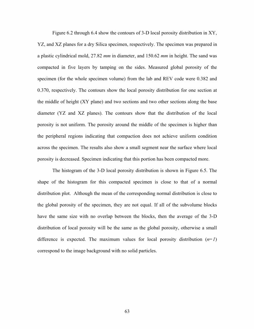
Figure 6.2 through 6.4 show the contours of 3-D local porosity distribution in XY,
YZ, and XZ planes for a dry Silica specimen, respectively. The specimen was prepared in
a plastic cylindrical mold, 27.82 mm in diameter, and 150.62 mm in height. The sand was
compacted in five layers by tamping on the sides. Measured global porosity of the
specimen (for the whole specimen volume) from the lab and REV code were 0.382 and
0.370, respectively. The contours show the local porosity distribution for one section at
the middle of height (XY plane) and two sections and two other sections along the base
diameter (YZ and XZ planes). The contours show that the distribution of the local
porosity is not uniform. The porosity around the middle of the specimen is higher than
the peripheral regions indicating that compaction does not achieve uniform condition
across the specimen. The results also show a small segment near the surface where local
porosity is decreased. Specimen indicating that this portion has been compacted more.
The histogram of the 3-D local porosity distribution is shown in Figure 6.5. The
shape of the histogram for this compacted specimen is close to that of a normal
distribution plot. Although the mean of the corresponding normal distribution is close to
the global porosity of the specimen, they are not equal. If all of the subvolume blocks
have the same size with no overlap between the blocks, then the average of the 3-D
distribution of local porosity will be the same as the global porosity, otherwise a small
difference is expected. The maximum values for local porosity distribution (n=1)
correspond to the image background with no solid particles.
63

Figure 6.2. 3-D local porosity distribution contours of a Silica sand specimen in XY plane
64

Figure 6.3. 3-D local porosity distribution contours of a Silica sand specimen in YZ plane
65

Figure 6.4. 3-D local porosity distribution contours of a Silica sand specimen in XZ plane
66

Figure 6.5. Histogram of 3-D local porosity distribution of a specimen of Silica sand
67

6.3 3-D Distribution of Local Porosity and Shear Bands Characterization
A combination of the developed techniques in chapter 5 and 3-D distribution of
the local porosity can be used to characterize the soil microstructure in real time.
Figure 6.6 shows a simple schematic diagram of the soil microstructure characterization
in real time. A triaxial sand specimen is loaded by using the designed triaxial apparatus in
chapter 4. A constant confining pressure is applied to the specimen for the whole period
of the test. Axial load is applied in a very slow rate in several different steps. At each step
loading is stopped and the specimen is scanned by X-ray CT. Scanning time is relatively
fast so that no further changes in the soil microstructure is expected. Loading and
scanning are continued until axial strain reaches to the final desired value (usually 20%).
Then the 3-D CT images are processed to find the 3-D distribution of local porosity and
displacement fields. Onset of formation of shear band and the related properties could be
determined from sudden jumps in the 3-D distribution of the local porosity. Shape and
orientation of the shear bands may be obtained directly from the 3-D X-ray CT images.
68

Figure 6.6. A summary of the shear band characterization procedure
69

Chapter 7
CONCLUSIONS AND RECOMMENDATIONS
7.1 Introduction
This study made use of the advances in X-ray computed tomography to generate
3-D images of the soil microstructure nondestructively. It has developed a systematic
method to examine the existence and the characteristics of the representative elementary
volume (REV) of a granular medium using X-ray CT. The study also developed a novel
triaxial apparatus to be placed inside the X-ray chamber to facilitate the real time
monitoring of the changes in sand microstructure when subjected to loading. Methods to
find the internal 3-D displacement fields based on two 3-D X-ray CT images are also
developed. The study concludes with the development of a method to quantify the 3-D
local porosity distribution in specimens. This chapter presents a summary of the
developments as well as some recommendations for future studies.
7.2 REV for Porosity of Sand
An interactive 3-D image-processing program was developed to process the 3-D
CT images and choose the REV. The effect of the shape and size of the particles,
specimen porosity, and location of the REV center were examined in this study using
different specimens of spherical glass beads, silica sand and Ottawa sand. The results
show the characteristic of three different regions; a microscopic fluctuations region,
constant region, and monotonically increasing/decreasing region.
70

The REV radius for the glass beads specimens and random packing is found to be
2 to 3 times of the identical average sphere diameter. The radius for silica sand
composed mainly of elongated particles is between 5 to 11 times of d50, and for Ottawa
sand composed mainly of subrounded particles is between 9 to 16 times of d50. These
values appear to justify the use of 10 to 20 diameters of sand grains adopted in some
studies. The fact that the radius of REV appears to decrease with elongation and
angularity leads us to the determination that interlocking may be a contributor in
determining its size.
The proposed method is general and it can be applied for any granular or
perforated material if the void sizes are more than the maximum CT image resolution.
However, at the present time the maximum specimen size is limited to the capabilities of
the X-ray CT equipment and available memory to process the image.
In view of its usefulness, the concept of REV relating to numerical modeling and
selection of specimen size for laboratory tests is debated very much lately. As discussed
in the introduction here, it is necessary to realize that REV concept is useful for getting
average properties of a homogenous medium. On the other hand, element tests on natural
media inevitably encounter heterogeneity and the classical continuum hypothesis breaks
down. In this case, the size of REV becomes scale-dependent. One may define a REV
size for a specific sized specimen in a laboratory-scale problem but this may not be
applicable to larger sized specimens or field-scale problems, where heterogeneity at
several scales exists. Additional non-local continuum measures are needed to fully
describe scale effects in such heterogeneous media (See Al Hattamleh et al. 2003).
71

7.2 X-Ray Triaxial System
By applying some modifications and using a small light-weight loading system a
novel triaxial system for real time monitoring of the soil microstructure was designed.
This novel triaxial apparatus designed so that it can be placed on the FlashCT stage to
generate the 3-D X-ray CT images of the soil microstructure in the time interval between
the two load increments. This novel triaxial can also be used to perform triaxial tests on a
wide range of different materials such as wood, asphalt, composites, ceramics, and
plastics. Based on the design requirements in this study, acrylic material is recommended
for the cell material.
7.3 3-D Internal Displacement Fields
The method of template matching to find the 2-D displacement fields between
two 2-D digital photographs was extended to find the 3-D displacement fields between
two 3-D X-ray CT images. An interactive computer program (M-DST) was developed to
load two 3-D CT images, find the displacement fields, and represent it as a vector field or
contour plots in three different planes.
The major problems with extension of this method for 3-D X-ray CT images are
fluctuations of the X-ray beam, limited computer memory to load two 3-D X-ray CT
images at the same time, and extremely long processing time. Fluctuation of the X-ray
intensity was fixed using large numbers of averaging captured frames to form each digital
radiograph. To overcome to the memory problem with loading of two 3-D X-ray CT
images at the same time, the method of successive read and write on the hard disk drive
was applied. Instead of searching the whole voxels of the current image, a search region
is defined in the computer code and in this way only the part of the image, which is
72

required for processing, is loaded in memory to avoid memory overflow. To speed up the
processing time, the computer code was developed so that user can install it on as many
as machines he wants to find the displacement fields for each part individually. The
results for each part are put together to have the displacement fields for the whole image.
7.4 3-D Local Porosity Distribution
3-D image processing techniques were used to find local porosity distribution. A
computer code was developed to find the local porosity distribution for 3-D X-ray CT
images. The 3-D X-ray CT image after segmentation is subdivided to smaller subvolumes
and porosity is determined for each subvolume. The program can represent the results in
form of filled contour plots or contour lines in three different planes (XY, XZ, and YZ) or
local porosity distribution histogram or as an AVI movie. The 3-D distribution of the
local porosity can also be saved in a 3-D array.
The results of 3-D local porosity distribution for Silica sand specimens prepared
in a plastic mold by compacting the sand in five layers and tamping on the sides showed
that porosity around the middle of the specimen is higher than the peripheral regions
indicating that compaction does not achieve uniform condition across the specimen. The
results also show a small segment near the surface where local porosity is decreased.
Specimen indicating that this portion has been compacted more.
The developed code can also be applied to characterize the shear band properties
for specimens are loaded inside the X-ray CT chamber. Onset of formation of shear band
and the related properties could be determined from sudden jumps in the 3-D distribution
of the local porosity.
73

7.5 Recommendations
This work has laid the foundation for development of nondestructive methods to
characterize the granular microstructure and its changes in real time combining X-ray CT
technology with robust image processing algorithms. This work should stimulate the
experimental studies that attempt to quantify strain localization and related phenomena
nondestructively.
The following recommendations are made for further research:
• Currently power of the X-ray CT and computer memory are two major issues that
limit the finding REV to small scales. However, with continued advances in X-ray
CT systems and computer hardware would push these limits and it would be
possible to find REV for larger scales.
• In case of large rotations a large amount of error is expected in determination of
3-D displacement fields. An optimization code may need to be added to M-DST
to consider rotation of the blocks.
• When the reference and the current image do not have the same size or there is
distortion in the target, then the cross-correlation method used here fails. In this
case a mathematical model such as hidden Markov models, which is widely used
for voice recognition and computer vision, is recommended to find 3-D
displacement fields.
• The time and delay in the triaxial device did not enable the real time experiments.
Experiments should be performed to characterize the features of strain
localization in granular materials.
74

• The current design of the triaxial apparatus is limited to sands. For the triaxial
testing of stronger materials such as concrete and rock would need a different
design as stronger and bigger jacks are required for imposing larger axial loads. In
this case the rotary stage will not be able to handle the heavy weight of both
triaxial apparatus and jack together and the alternate design in Appendix C is
recommended.
75
REFERENCES
Aifantis, E. C. (1987). “Physics of Plastic Deformation”. International Journal of
Plasticity, Vol. 3, No. 3, pp. 2ll-247. Al Hattamleh, O. (2003). Investigation Of The Deformation Of Granular Materials: A
Micromechanics Approach. Ph. D. Thesis. Washington State University. Al Hattamleh, O., Muhunthan, B., and Zbib, H. M. (2004). “Gradient Plasticity Modeling
of Strain Localization in Granular Materials”. International Journal for Numerical and Analytical Methods in Geomechanics, No. 28, pp. 465-481.
Al Hattamleh, O. (2003-2005). Personnel Communication. Washington State University.
Al Ramahi, B. (2004). Characterization of Shearing Phenomenon and Porosity of Porous Media using X-Ray Computed Tomography. MSc. Thesis. Louisiana State University.
Al Raoush, R. I. and Willson, C. S. (2005). “A Pore-Scale Investigation of a Multiphase
Porous Media System”. Journal of Contaminant Hydrology, Vol. 77, No. 1-2, pp. 67-89.
Al Raoush, R. I. and Alshibli, K. A. (2006). “Distribution of Local Void Ratio in Porous
Media Systems from 3-D X-Ray Microtomography Images”. Physica A: Statistical Mechanics and its Applications, Vol. 359, No. 1-4, pp. 713-728.
Alshibli, K. A. and Sture, S. (1999). “Sand Shear Band Thickness Measurements by
Digital Imaging Techniques”. Journal of Computing in Civil Engineering, Vol. 13, No. 2, pp. 103-109.
Alshibli, K. A., Sture, S., Costes, N. C., Frank, M. L., Lankton, M. R., Batiste, S. N., and
Swanson, R. A. (2000). “Assesment of Localized Deformations In Sand Using X-Ray Computed Tomography”. ASTM Geotechnical Testing Journal, Volume 23, No. 3, pp. 274-299.
Alshibli, K. A., Batiste, S. N., Swanson, R. A., Sture, S., Costes, N. C., and Lankton, M.
R. (2000). “Quantifying void ratio variation in sand using computed tomography Source”. Geotechnical Special Publication, No. 106, pp. 30-43.
Alshibli, K. A. and Sture, S. (2000). “Shear Band Formation in Plane Strain Experiments
of Sand”. Journal of Geotechnical and Geoenvironmental Engineering, Vol. 126, No. 6, pp. 495-503.
76

Alshibli, K. A., Batiste, S. N., and Sture, S. (2003). “Strain Localization in Sand: Plane Strain versus Triaxial Compression”. Journal of Geotechnical and Geoenvironmental Engineering, Vol. 129, No. 6, pp. 483-494.
Alshibli, K. A. and Al Ramahi, B. (2006). “Microscopic Evaluation of Strain
Distribution in Granular Materials During Shear”. Journal of Geotechnical and Geoenvironmental Engineering, Vol. 132, No. 1, pp. 80-91.
ASTM Standard E 1441–00, Standard Guide for Computed Tomography CT Imaging,
Annual Book of ASTM Standards, Nondestructive Testing, Vol. 03.03, ASTM International, West Conshohocken, PA, 2005.
Auzerais, F. M., Dunsmuir, J., Ferreol, B. B., Martys, N., Olson, J., Ramakrishnan, T. S.,
Rothman, D. H., and Schwartz, L. M. (1996). “Transport in Sandstone: A Study Based on Three Dimensional Microtomography”. Geophysical Research Letters, Vol. 23, No. 7, pp. 705-708.
Batiste, S. N., Alshibli, K. A.; Sture, S., and Lankton, M. (2004). “Shear Band
Characterization of Triaxial Sand Specimens using Computed Tomography”. Geotechnical Testing Journal, Vol. 27, No. 6, pp. 568-579.
Bazant, Z. P. and Gambarova, P. G. (1984). “Crack Shear in Concrete: Crack Band
Microplane Model”. Journal of Structural Engineering, Vol. 110, No. 9, pp. 2015-2035.
Bear, J. (1972). Dynamics of Fluids in Porous Media, American Elsevier Publisher Co.,
New York. Budhu, M. (1984). “On Comparing Simple Shear and Triaxial Test Results”. Journal of
Geotechnical Engineering, Vol. 110, No. 12, pp. 1809-1814. Chang, C. S., Matsushima, T., and Lee, X. (2003). “Heterogeneous Strain and Bonded
Granular Structure Change in Triaxial Specimen Studied by Computer Tomography”. Journal of Engineering Mechanics, ASCE, Vol. 129, No. 11, pp. 1295-1307.
Charbeneau, R. J. (2000). Groundwater Hydraulics and Pollutant Transport. Prentice
Hall, New Jersey. Cislerova, M. and Votrubova, J. (2002). “CT Derived Porosity Distribution and Flow
Domains”. Journal of Hydrology, Vol. 267, No. 3-4, pp. 186-200. Clausnitzer, V. and Hopmans, J. W. (1999). “Determination of Phase-Volume Fractions
from Tomographic Measurements in Two-Phase Systems”. Advances in Water Resources, Vol. 22, No. 6, pp. 577-584.
77

Clocksin, W. F., Quinta Da Fonseca, J., Withers, P. J., and Torr, P. H. S. (2002). “Image Processing Issues in Digital Strain Mapping”. Proceedings of SPIE-The International Society for Optical Engineering, Vol. 4790, pp. 384-395.
Culligan, K. A., Wildenschild, D., Christensen, B. S. B., Gray, W. G., Rivers, M. L., and
Tompson, A. F. B. (2004). “Interfacial Area Measurements for Unsaturated Flow through a Porous Medium”. Water Resources Research, Vol. 40, No. 12, pp. 1-12.
Dagher, H. J., Abdel-Magid, B., Ritter, M., and Iyer, S. (1997). “GRP Prestressing of
Wood Decks”. Proceeding of Structure Congress XV, ASCE, Portland, Oregon, pp. 585-589.
de Borst, R. and Muehlhaus, H. B. (1992). “Gradient-Dependent Plasticity: Formulation
and Algorithmic Aspects”. International Journal for Numerical Methods in Engineering, Vol. 35, No. 3, pp. 521-539.
Dennis, M. J. (1989). “Industrial Computed Tomography”. Reprinted from Metals
Handbook, Vol. 17, pp. 358–386. Desrues, J. and Chambon, R. (1989). “Shear band analysis for granular materials: the
question of incremental non-linearity”. Ingenieur-Archive, Vol. 59, No. 3, pp. 187-196.
Desrues, J., Chambon, R.; Mokni, M., and Mazerolle, F. (1996). “Void ratio Evolution
inside Shear Bands in Triaxial Sand Specimens Studied by Computed Tomography”. Geotechnique, Vol. 46, No. 3, pp. 529-546.
Desrues, J. and Viggiani, G. (2004). “Strain Localization in Sand: An Overview of the
Experimental Results Obtained in Grenoble using Stereophotogrammetry”. International Journal for Numerical and Analytical Methods in Geomechanics, Vol. 28, No. 4, pp. 279-321.
Desrues, J. and Hammad, W. (1989). “Shear Banding Dependency on Mean Pressure Level in Sand”. International workshop on Numerical Methods for Localization and Bifurcation of Granular Bodies, Gdansk, Poland.
Dullien, F. A. L. (1979). Porous Media: Fluid Transport and Pore Structure, Academic Press, NewYork.
Eaton, D. (2006). “Fast NCC”. http://www.cs.ubc.ca/~deaton/remarks_ncc.html.
Finno, R. J., Harris, W. W., Mooney, M. A., and Viggiani, G. (1996). “Strain Localization and Undrained Steady State”. Journal of Geotechnical Engineering, ASCE, Vol.122, No. 6, pp. 462-473.
78

Finno, R. J., Harris, W. W., Mooney, M. A., and Viggiani, G. (1997). “Shear Bands in Plane Strain Compression of Loose Sand”. Geotechnique, Vol. 47, No. 1, pp. 149-165.
Fleck, N. A. and Hutchinson, J. W. (1993). “Phenomenological Theory for Strain
Gradient Effects in Plasticity”. Journal of the Mechanics and Physics of Solids, Vol. 41, No. 12, pp. 1825-1857.
Ge, X., Ren, J., Pu, Y., Ma, W., and Zhu, Y. (1999). “Real-in-Time CT Triaxial Testing
Study of Meso-Damage Evolution Law of Coal”. Yanshilixue Yu Gongcheng Xuebao/Chinese Journal of Rock Mechanics and Engineering, Vol. 18, No. 5, pp. 497-502.
Geraud, Y. (1991). Deformations Thermomecaniques et Porosite des Roches
Granitiques. Evolution des Espaces Poreux, Thesis doct., University of Maseilles. Geraud, Y., Mazerolle, F. Raynaud, S., and Lebon, P. (1998). “Crack Location in Granite
Samples Submitted to Heating, Low Confining Pressure and Axial Loading”. International Journal of Geophysics, No. 133, pp. 553-567.
Gonzalez, R. C., Woods, R. E., and Eddins, S. L. (2004). Digital Image Processing using
Matlab, Prentice Hall. Graton, L. C. and Fraser, H. J. (1935). “Systematic Packing of Spheres with Particular
Relation to Porosity and Permeability,” Journal of Geology, Vol. 43, No. 8, pp. 785–909.
Gudehus, G. and Nubel, K. (2004). “Evolution of Shear Bands in Sand”. Geotechnique,
Vol. 54, No. 3, pp. 187-201. Guler, M., Edil, T. B., and Bosscher, P. J. (1999). “Measurement of Particle Movement in
Granular Soils using Image Analysis”. Journal of Computing in Civil Engineering, Vol. 13, No. 2, pp. 116-122.
Han, C. and Drescher, A. (1993). “Shear Bands in Biaxial Tests on Dry Coarse Sand”.
Soils and Foundations, Vol. 33, No. 1, pp. 118-132. Haralick, R. M. and Shapiro, L. G. (1993). Computer and Robot Vision, Vol. II, Addison-
Wesley Publishing Company, Inc. Horii, H., Takamatsu, K., Inoue, J., and Sasaki, N. (1998). “Measurement of
Displacement Field by Match Method and Observation of Strain Localization in Soft Rock”. Proceeding of Second International Conference on Imaging Technologies: Techniques and Applications in Civil Engineering, ASCE, Reston, VA, pp. 10-19.
79

HYTEC INC, 2004, FlashCT User’s Manuals, Los Alamos, NM. Kak, A. C. and Slaney, M. (2001). Principle of Computerized Tomographic Imaging,
Siam, Philadelphia, PA. Klobes, P., Riesemeier, H., Meyer, K., Goebbels, J., Siitari-Kauppi, M., and Hellmuth, K.
H. (1997). “Investigation of Rock Samples using X-Ray Microcomputer-Tomography before and after Mercury Intrusion Porosimetry”. Materials Research Society Symposium - Proceedings, Vol. 465, Scientific Basis for Nuclear Waste Management XX, pp. 863-870.
Lawler, J., and Shah, S. (2002). “Fracture Process in Concrete Studied with Subregion
Scanning Computer Vision”. The 15th Engineering Mechanics Division Conf., ASCE, Reston, VA.
Lewis, J. P. (1995). “Fast Normalized Cross-Correlation”. Industrial Light & Magic,
http://www.idiom.com/~zilla/Papers/nvisionInterface/nip.html. Li, X. J. and Zhang, D. L. (2000). “Monitoring Change of Structure of Road Foundation
Soil in Uniaxial Compression Test with CT”. Chinese Journal of Geotechnical Engineering, Vol. 22, No. 2, pp. 206-209.
Liu, J. and Iskander, M. (2004). “Adaptive cross correlation for imaging displacements in
soils”. Journal of Computing in Civil Engineering, Vol. 18, No. 1, pp. 46-57. Lu, Z. H., Chen, Z. H., and Pu, Y. B. (2002). “Study on Damage Evolution of Natural
Expansive Soil with Computerized Tomography during Triaxial Shear Test”. Chinese Journal of Hydraulics Engineering, No. 6, pp. 106-112.
Masad, E. and Muhunthan, B. (2000). “Three-Dimensional Characterization and
Simulation of Anisotropic Soil Fabric”. Journal of Geotechnical and Geoenvironmental Engineering, Vol. 126, No. 3, pp. 199-207.
Masad, E., Button, J. W., and Papagiannakis, T. (2000). “Fine-aggregate angularity:
Automated image analysis approach”. Transportation Research Record, No. 1721, pp. 66-72.
MathWorks, 2004, Image Processing Toolbox for Use with MATLAB User’s Guide,
Version 5, Natick, MA. Meegoda, N. J., King, I. P., and Arulanandan, K. (1989). “Expression for the
Premeability of Anisotropic Granular Media”. International Journal for Numerical and Analytical Methods in Geomechanics, Vol. 13, No. 6, pp. 575-598.
Mindlin, R. D. (1964). “Microstructure in Linear Elasticity”. Archive for Rational Mechanics and Analysis, Vol. 10, Issue 1, pp.51-78.
80

Muhunthan, B. Chameau, J. L. and Masad, E. (1996). “Fabric Effects on the Yield Behavior of Soils”. Soils and Foundations, JSGE, Vol. 36, No. 3, pp. 85-97.
Nemat-Nasser, S. and Okada, N. (2001). “Radiographic and Microscopic Observation of Shear Bands in Granular Materials”. Geotechnique, Vol. 51, No. 9, pp. 753-765.
Oda, M., Konishi, J., and Nemat-Nasser, S. (1982). “Experimental Micromechanical
Evaluation of Strength of Granular Materials: Effect of Particle Rolling”. Mechanics of Materials, Vol. 1, No. 4, pp. 269-283.
Oda, M. and Kazama, H. (1998). “Microstructure of Shear Bands and Its Relation to the
Mechanisms of Dilatancy and Failure of Dense Granular Soils”. Geotechnique, Vol. 48, No. 4, pp. 465-481.
Oda, M., Takemura, T., and Takahashi, M. (2004). “Microstructure in Shear Band
Observed by Microfocus X-ray Computed Tomography”. Geotechnique, Vol. 54, No. 8, pp. 539-542.
Ostoja-Starzewski, M. (2005). “Scale Effects in Plasticity of Random Media: Status and
Challenges”. International Journal of Plasticity, Vol. 21, No. 6, pp. 1119-1160. Otani, J., Mukunoki, T., and Obara, Y. (2000). “Application of X-ray CT Method for
Characterization of Failure in Soils”. Soils and Foundations, Vol. 40, No. 2, pp. 111-118.
Otani, J. and Mukunoki, T. (2001). “Development of New Triaxial Compression Test
Apparatus for Geomaterials on Industrial X-Ray CT Scanner”. Proceeding of XVth International Conference on Soil Mechanics and Geotechnical Engineering. pp. 231-234.
Otani, J. and Mukunoki, T. (2001). “Development of New Triaxial Compression Test
Apparatus for Geomaterials on Industrial X-Ray CT Scanner”. Proceeding of XVth International Conference on Soil Mechanics and Geotechnical Engineering, pp. 231-234.
Otsu, N. (1979). “Threshold Selection Method from Gray-Level Histograms”. IEEE
Transactions on Systems, Man and Cybernetics, Vol. SMC-9, No. 1, pp. 62-66.
Pradhan, T. (1997). “Characteristics of Shear Band in Plane Strain Compression Test of Sands”. In Deformation and Progressive Failure in Geomechanics, Asaoka A, Adachi T, Oka F. (eds). Pergamon, Oxford, pp. 241-246.
Rechenmacher, A., and Saab, N. (2002). “Digital Image Correlation (DIC) to Evaluate Progression and Uniformity of Shear Bands in Dilative Sands”. Proceedings of the15th Engineering Mechanics Division Conference, ASCE, Reston, Va.
81

Roberts, A. J., (1994). A One-Dimensional Introduction to Continuum Mechanics, World Scientific Publishing Co., Singapore.
Russ, J. C., (2002). The Image Processing Hand Book, CRC Press, Boca Raton, FL. Saada, A. S., Bianchini, G. F., and Liang, L. (1994). “Cracks, Bifurcation and Shear
Bands Propagation in Saturated Clays”. Geotechnique, Vol. 44, No. 1, pp. 35-64. Saada, A. S., Liang, L., Figueroa, J. L., and Cope, C. T. (1999). “Bifurcation and Shear
Band Propagation in Sands”. Geotechnique, Vol. 49, No. 3, pp. 367-385. Sadek, S., Iskander, M., and Liu, J. (2002). “Geotechnical Properties of Transparent
Silica”. Canadian Geotechnical Journal, Vol. 39, No. 1, pp. 111-124. Sadek, S., Iskander, M., and Liu, J. (2003). “Accuracy of Digital Image Correlation for
Measuring Deformations in Transparent Media”. Journal of Computing in Civil Engineering, Vol. 17, No. 2, pp. 88-96.
Schanz, T., Desrues, J., and Vermeer, P. A. (1997). “Comparison of Sand Data on
Different Plane Strain Devices”. In Deformation and Progressive Failure in Geomechanics, Asaoka A, Adachi T, Oka F. Pergamon, Oxford, pp. 289-295.
Shah, S. P. and Choi, S. (1996). “Evaluation of Fracture Processes in Cement-Based
Materials under Compression Using Computer Vision”. American Society of Mechanical Engineers, Materials Division (Publication) MD, Vol. 74, pp. 25-26.
Shi, B., Murakami, Y., Wu, Z., Chen, J., and Inyang, H. (1999). “Monitoring of Internal
Failure Evolution in Soils using Computerization X-ray Tomography”. Engineering Geology 54, pp. 321-328.
Spanne, P., Jones, K. W., Prunty, L., and Anderson, S. H. (1994). “Potential
Applications of Synchrotron Computed Microtomography to Soil Science”. SSSA Special Publication, No. 36, pp. 43-57.
Spanne, P., Thovert, J. F., Jacquin, C. J., Lindquist, W. B., Jones, K. W., and Adler, P. M.
(1994). “Synchrotron Computed Microtomography of Porous Media: Topology and Transports”. Physical Review Letters, Vol. 73, No. 14, pp. 2001-2004.
Stroeven, M., Askes, H., and Sluys, L. J. (2004). “Numerical Determination of
Representative Volumes for Granular Materials”. Computer Methods in Applied Mechanics and Engineering, Vol. 193, No. 30-32, pp. 3221-3238.
Sun, H., Chen, J. F., and Ge, X. R. (2004). “Deformation Characteristics of Silty Clay
Subjected to Triaxial Loading, by Computerised Tomography”. Geotechnique, Vol. 54, No. 5, pp. 307-314.
82

Tani, K. (1997). “X-Ray Computed Tomography Technique to Observe Shear Banding in Dense Sands. Deformation and Failure in Geomechanics”. IS Nagoya ’97, Pergamon, pp. 315-320.
Vardoulakis, I. (1980). “Shear Band Inclination and Shear Modulus of Sand in Biaxial
Tests”. International Journal for Numerical and Analytical Methods in Geomechanics, Vol. 4, No. 2, pp. 103-119.
Vardoulakis, I. and Aifantis, E. C. (1989). Gradient Dependent Dilatancy and Its
Implications in Shear Banding and Liquefaction”. Ingenieur-Archiv, Vol. 59, No. 3, pp. 197-208
Vardoulakis, I. (1996). “Deformation of Water-Saturated Sand: I. Uniform Undrained
Deformation and Shear Banding”. Geotechnique, Vol 46, No. 3, pp. 441-456. Viggiani, G., Lenoir, N., Besuelle, P., Michiel, M. D., Marello, S., Desrues, J., and
Kretzschmer, M. (2004). “X-ray Microtomography for Studying Localized Deformation in Fine-Grained Geomaterials under Triaxial Compression”. C. R. Mecanique 332, Elsevier, pp. 819-826.
Vinegar, H. J., De Waal, J. A., and Wellington, S. L. (1991). “CT Studies of Brittle
Failure in Castlegate Sandstone”. International Journal of Rock Mechanics and Mining Sciences & Geomechanics Abstracts, Vol. 28, No. 5, pp. 441-450.
Walton, K. (1987). “Effective Elastic Moduli of a Random Packing of Spheres”. Journal
of the Mechanics and Physics of Solids, Vol. 35, No. 2, pp. 213-226. Wang, Q. and Lade, P. V. (2001). “Shear Banding in True Triaxial Test and Its Effect on
Failure in Sand”. Journal of Engineering Mechanics, Vol. 127, No. 8, pp. 754-761.
Wang, L. B., Frost, J. D., and Lai, J. S. (2004). “Three-Dimensional Digital
Representation of Granular Material Microstructure from X-ray Tomography Imaging”. Journal of Computing in Civil Engineering, ASCE, Vol. 18, No.1, pp. 28-35.
White, D., Take, W., and Bolton, M. (2001). “Measuring Soil Deformation in
Geotechnical Models Using Digital Images and PIV Analysis”. Proceedings of the 10th International Conference on Computer Methods and Advances in Geomechanics, Tuscon, AZ, Balkema, Rotterdam, The Netherlands, pp. 997-1002.
White, D. J. and Bolton, M. D. (2004). “Displacement and Strain Paths During Plane-
Strain Model Pile Installation in Sand”. Geotechnique, Vol. 54, No. 6, pp. 375-397.
83

Wood, D. M. (2002). “Some Observations of Volumetric Instabilities in Soils”. International Journal of Solids and Structures 39, Pergamon, pp. 3429-3449.
Yagi, K., Miura, S., Asonuma, T., Sakon, T., and Nakata, T. (1997). “Particle Crushing
and Shear Banding of Volcanic Coarse-Grained Soils”. In Deformation and Progressive Failure in Geomechanics, Asaoka A., Adachi T., Oka F. (eds). Pergamon; Oxford, pp. 139-145.
Yoshida, T., Tatsuoka, F., and Siddiquee, M. (1994). “Shear Banding in sands Observed in Plane Strain Compression”. Localization and Bifurcation theory for Soils and Rocks, Chambon R., Desrues J., Vardoulakis I. (eds). Balkema, Rotterdam, pp. 165-181.
Zbib, H. M. and Aifantis, E. C. (1988). “On the Concept of Relative and Plastic Spins and Its Implications to Large Deformation Theories. Part II: Anisotropic Hardening Plasticity”. Acta Mechanica, Vol. 75, pp. 35-56.
Zhou, Z., Synolakis, C. E., Leahy, R. M., and Song, S. M. (1995). “Calculation of 3-D
Internal Displacement Fields from 3-D X-ray Computer Tomographic Images”. Proceedings: Mathematical and Physical Sciences, Vol. 449, No. 1937, pp. 537-554.
84

Appendix A
X-RAY COMPUTED TOMOGRAPHY
A.1 Introduction
X-ray Computed tomography (X-ray CT), in a general sense, is an imaging
technique that generates an image of density distribution of a thin cross-section of a
specimen. Computed tomography imaging is also known as CAT scanning (Computed
Assisted Tomography). Tomography is from the Greek word "tomos" meaning "slice" or
"section" and “graphia” meaning, "describing". Computed tomography was invented by
the British Engineer Godfrey Hounsfield of EMI Laboratories in the late 1960’s and early
1970’s in England, and independently by South African born physicist Allan
M. Cormack (1963) of Tufts University, Massachusetts. Since then X-ray CT has made
great improvements in speed, quality, and resolution.
The X-ray CT image represents the point-by-point linear attenuation coefficients
in the slice, which depends on the physical density of the material, the effective atomic
number of the material, and the X-ray beam energy. X-ray CT image is highly sensitive
to small differences (less than 1%) in density (Dennis 1989). Computed tomography
system can also produce digital radiography images (DR). Both DR and CT images may
be further processed. A digital radiography image is a digital attenuation image, which
formed by placing the specimen between the X-ray source and the detector.
Consequently, in DR all points are projected on a 2-D plane and finding the 3-D
coordinates of a point form a DR is almost impossible. On the other hand, in CT images
85

the coordinates of every point are known and this is the major difference between a DR
image and a CT image (Figures A.1 and A.2). A series of CT images can be used to
characterize the object volume. The 3-D image is formed by voxels, which are box-
shaped volume defined by the area of the pixel and the height of the slice thickness
(Appendix B).
(a) (b)
Figure A.1. Difference between (a) digital radiograph and (b) 3-D X-ray CT image of a
cylindical soil sample
86

(a) (b)
Figure A.2. Difference between (a) digital radiograph and (b) X-ray CT image of a
reinforced composite specimen (middle slice)
A.2 Principles of X-ray CT
The CT scanning system contains a radiation source and a linear array radiation
detector with a precision stage to scan cross-sectional slice from different angles. The
detector usually consists of a series of individual X-ray sensors arranged in lines and
columns. X-ray beam may be in any of these forms; parallel beam, fan beam, and cone
beam depending on the geometric shape. However, the beam must be wide enough to
expose all the detector elements. The pixels on the detector measure the energy of the
X-ray beam, which can be related to the numbers of photons. Subsequently, the acquired
data are sent to the computer to produce the CT image. The CT image reconstruction
algorithm generates two-dimensional images in horizontal planes from a set of digital
radiographs taken at different angels. Though the whole processes of data acquisition,
reconstruction, and post processing are done by the X-ray CT Software, knowing the
basic principles of computed tomography and the meaning of important terms in X-ray
87

CT are necessary. Therefore, a brief description of the important terminology is provided
next for completeness.
A.2.1 CT Numbers (H)
The resulting images of CT are grey scale images; usually white color indicates
the highest density and black the lowest density (Figures A.3 and A.4). Each shade is
related to a CT number or Hounsfield unit (Hounsfield 1973):
−=
wx
xw
x
HNumberCTµ
µµ1000)( (A.1)
where
= linear attenuation coefficient xµ
= linear attenuation coefficient of the water xwµ
The scaling of the linear attenuation coefficient into an integer pixel value, as well
as the range of CT number scales, is somewhat arbitrary among the different systems.
For example, in medical CT systems the CT number of water is assumed zero and is
considered as a reference for other CT numbers. On the other hand, in industrial CT
systems the CT number of air is normally set the value 0. Note that no standard scaling
of the CT values is applicable to all different materials and X-ray energies used. The
value corresponds to water and the value 0=H 1000−=H corresponds to ,
which is assumed to be the attenuation coefficient of air.
0=xµ
88

The projection data values for a narrow mono-energetic beam of X-ray radiation
can be theoretically modeled by considering first Lambert’s law of absorption:
(A.2) )exp(0 sII xµ−=
where I is the intensity of the beam transmitted through the absorber, is the initial
intensity of the beam, is the thickness of the absorber, and is the linear attenuation
coefficient of the absorber material.
0I
s xµ
Figure A.3. 3-D X-ray CT image of a battery and distribution of CT numbers
89

Figure A.4: Variation of CT numbers along the diameter of a soil sample
A.2.2 CT Image Quality
Spatial resolution, image contrast, and image artifacts are three basic factors
affecting image quality. Spatial resolution is a measure of the ability of an imaging
system to identify and distinguish small details. For example, the X-ray CT system at
Washington State University can reach a spatial resolution up to 5 micron under certain
conditions (high enough to detect sand particles). The amount of the contrast on a X-ray
CT image is governed by object contrast, which refers to the contrast generated by
variations in the attenuations of the radiation propagating through the specimen, the
contrast resolution of the detector-readout system, and the size of discontinuity with
respect to the special resolution of the system.
Artifacts are image features that do not correspond to physical structures in the
object. All imaging techniques are subject to certain types of artifacts. In general the two
90

major causes of X-ray CT image artifacts are the finite amount of data for generating the
constructed image, and the systemic errors in CT process and hardware. Inaccuracies in
geometry, beam hardening (the increase in effective energy of a
poly-energetic X-ray beam with increasing the attenuation of the beam), aliasing (an
artifact in discretely measured data cause by insufficient sampling of high-frequency
data, with this high frequency information falsely recorded at a lower frequency), and
partial penetration are some of the other factors known to cause artifact. For instance the
straight lines and noisy circles in Figure A.5 are artifacts on a CT slice of a battery.
Figure A.5. Artifacts (straight lines and noisy circles) on a X-ray CT slice of a battery
A.2.3 Computed Tomography Reconstruction Techniques
To reconstruct a CT image, first the measured radiation intensities are converted
into the projection data that correspond to the sum or projection of X-ray densities along
a ray path. Subsequently, the point-by-point distribution of the X-ray densities in the
two-dimensional image of the cross-sectional slice is determined by processing of the
91

projection data with a reconstruction algorithm. These are the basic steps of
reconstruction process. There are many different reconstruction algorithms available for
computed tomography. Most, however, are based on two basic methods: transform
methods and iterative methods. The two main types of transform methods are Fast
Fourier Transform (FFT) and Filtered Back-Projection. In industrial X-ray CT systems to
process large image sizes, the Filtered Back Projection technique is the most commonly
used method.
Calculation of projection data is the first step in the reconstruction of a CT image.
The measured intensity data are normalized by the corresponding intensity obtained
without presence of the object. The projection data values correspond to the sum of the
linear attenuation coefficients values along the line of the transmitted radiation.
The linear attenuation coefficients of the material distribution in a
two-dimensional section can be expressed by the function, , where x and y are
the Cartesian coordinates specifying the location of points in the section. The intensity of
radiation transmitted along a particular path is given by:
),( yxxµ
−= ∫ −
ector
sourcerayx
x dsyxIIdet
0 ),(exp µ (A.3)
where is the differential of the path length along the ray. Reconstruction program in a
X-ray CT system determines the distribution of from a series of intensity
measurements through the section. This equation may be rewritten in the form of Radon
transformation of equation, to give projection value, :
ds
),( yxxµ
),( yxxµ xp
∫ −=
=
ector
sourcerayx
xx dsyxIIp
det0 ),(ln µ (A.4)
92

The above Radon transformation of equation is fundamental to the CT
process. Radon (1917) showed that can be determined analytically from a given
finite set of projection values (Appendix B).
),( yxxµ
),( yxxµ
A.2.3.1 Fourier Transform Reconstruction Technique
A Fourier transform is a mathematical operation that converts the object
distribution defined in special coordinates into equivalent sinusoidal amplitude and phase
distribution in special frequency coordinates (Appendix B). It is used as a reconstruction
technique. The one-dimensional Fourier transformation of a set of projection data at a
particular angle,θ , is described by:
( )drrrpP xx ∫∞+
∞−−= πρθθρ 2exp),(),( (A.5)
where r is the spatial position along the set of projection data and ρ is the corresponding
spatial frequency variable.
Central slice theorem is the basis of both Fourier transform reconstruction
technique and filtered-backprojection method. This theorem states that the Fourier
transform of a one-dimensional projection through two-dimensional distribution is
mathematically equivalent to the values along a radial line through a two-dimensional
Fourier transform of the original distribution. Taking the inverse two-dimensional Fourier
transform yields the object distribution in spatial coordinates.
A.2.3.2 Filtered-Backprojection Technique
As mentioned earlier the Filtered Backprojection Technique (FBP) is the most
commonly used CT reconstruction algorithm. Filtering operations, such as image
93

smoothing or sharpening, can be performed on the data in the spatial frequency domain.
Backprojection is the mathematical operation of mapping the one-dimensional projection
data back into a two-dimensional grid. It means that a visible structure in two or more
images taken at different angles can backproject along the corresponding ray paths to
determine the intersection of the rays and the location of the structure in space.
According to the central slice theorem the Fourier transform of the
one-dimensional projection data through a two-dimensional distribution is equivalent to
the radial values of the two-dimensional Fourier transform of the distribution.
Consequently, the filtering operation can be performed on the projection data prior to
backprojection. This is the conceptual basis of the filtered backprojection technique and it
is a useful method for reconstructing the large image sizes.
A 3-D X-ray CT image is formed by a stack of 2-D reconstructed slices in equal
distances (Figure A.6). The gaps between the 2-D slices are filled by finding the intensity
of gap voxels using a linear interpolation.
Figure A.6. A pile of 2-D reconstructed slices to generate a 3-D CT image
94

A.3 X-Ray CT System at Washington State University
The CT scans for this study are performed at the Washington State University
High Resolution X-ray Tomography facility. The facility consists of Flat panel
amorphous silicon high-resolution computed Tomography or FlashCT (Figure A.7).
FlashCT is an advanced high-speed 3rd generation industrial X-ray CT based 3-D
scanning system for nondestructive testing and evaluation. FlashCT is suitable for use
within a wide spectrum of X-ray energies and geometric magnifications.
Washington State University’s FCT-4200 is a novel design that incorporates both
an X-tek 225 keV micro-focus X-ray source for material characterization at high
magnification and a Pantak/Seifert 420 keV X-ray source for larger component analysis
housed in a single radiation cabinet enclosure (Figures A.8). The micro-focus X-ray
source takes advantage of an electromagnetic field and a vacuum pump around the X-ray
outlet to reduce the X-ray spot size. The detector employed is a Varian PaxScan 2520
with CsI scintillator. The distance between adjacent pixels (pixel spacing) on the detector
is 127 µm. With the wide energy spectrum and high magnification available, the
FCT-4200 can image a large variety of sample shapes, sizes, and densities. The X-ray CT
components are placed in a protective cabinet against X-ray with external cabinet
dimensions of 2.37 m (L) × 1.27 m (W) × 2.06 m (H). The walls of the cabinet have been
built using two 3 mm thick steel plates, which a 12 mm thick lead plate has been placed
between those plates. The thickness of the wall behind the detector is significantly more.
Because of the limited dimensions of the protective cabinet, and also the other
components inside, there is only a limited room for the specimens or any other
instrument.
95

Figure A.7. FlashCT facility at Washington State University
Figure A.8. Main components of FlashCT (or any other X-ray CT system in general)
96

A.4 X-Ray CT Scanning Procedure
Though the X-ray CT systems are very different, the scanning procedures are
almost the same. The major steps to scan an object are:
1. Specimen size with respect to the effective atomic number of the object
material, size of the stage, required resolution, and power of the X-ray source
is examined to ensure such that scan is possible. This depends on many
different variables and experience has the main role. However, most of the
times a few scans prior to the main scan are performed to ensure that the CT
image meet the requirements.
2. The object is fixed on the stage located between X-ray source and detector.
The distance between object and X-ray source (or object and detector) is
normally set based on the desired spatial resolution. If the distance between
the X-ray source and detector, pixel spacing of the detector, and desired
spatial resolution are assumed to be d, PS, and SR, respectively, then the
distance between the object and the X-ray source, dsource, is obtained by
Equation A.6. However, it is important to note that the maximum spatial
resolution is limited to the system specifications. If the image size exceed than
the detector, then dsource must be increased until the whole image fits in the
detector.
PSSRdd source = (A.6)
97

3. X-ray detector is calibrated, which for the number of photons that it counts for
two different conditions; when the X-ray is off (dark field calibration) and
when the X-ray is on with no object in the way of X-ray beam (light or gain
field calibration). For light field calibration it is recommended to use close
values to the scan values for X-ray current and intensity. No good quality
image is obtained unless a good calibration is performed prior to the scan.
Calibration may be repeated several times for the best result.
4. Rotary stage rotates the specimen a small angel then stops and a digital
radiograph is taken. This process is continued to complete a full circle
rotation.
5. 2-D CT slices are reconstructed from digital radiographs, and finally the 3-D
CT image is formed by a stack of 2-D slices.
98

Appendix B
AN OVERVIEW OF DIGITAL IMAGE PROCESSING
B.1 Digital Image
A digital image is a discrete function. Its domain is the set of positive integer
numbers and its range can be either the set of positive integer numbers (gray scale
images) or the set of rational numbers between 0 and 1 including both 0 and 1 (RGB
images). The elements of digital images are called pixel and voxel for two dimensional
and three dimensional digital images, respectively. Pixels are small square shaped
elements arranged in rows and columns that form the domain of the image. Voxels are
small box shaped elements, formed by extruding a pixel to a finite imaginary thickness.
In other words, voxels are extension of a planar element to a volume element to form
three dimensional digital images.
(a) (b)
Figure B.1. (a) A 2-D image and a magnified pixel (b) A 3-D image and a magnified
voxel
99

The value of each pixel or voxel represents the intensity or amplitude of the image
at that point. The intensity range for a gray scale image depends on the number of bits
(the smallest part of the memory, which is either 0 or 1) in a byte. The image is referred
to the number of bits in a byte. If the image consists of two colors only, black and white,
then 1 can be considered for white and 0 for black. In this case one bit in a byte is
enough to show those two colors. As such those images are called logical images.
To have different gray shades between black and white the number of bits in a
byte must be increased. In an 8-bit gray scale image, each bit can be either 0 or 1, so the
total number of possible gray shades will be 28 or 256 gray shades from black
(00000000) to white (11111111). Figure B.2(a) shows an 8-bit gray scale image with the
spectrum of the gray shades and Figure B.2(b) shows a logical (1-bit) image of the same
image. Representation the different gray shades, using 8 bits in each byte, is shown in
Figure B.3. In the same manner the total number of possible shades for a 16-bit and 32-
bit gray scale images are 65,536, and 4,294,967,296.
For most applications 8 to 16 bits are sufficient and increasing the number of
shades does not provide more accuracy or better quality. In practice and for most
applications there is no significant difference between 8-bit, 16-bit, and 32-bit images;
however a raw 16-bit image needs 256 times more memory than a raw 8-bit image, and a
raw 32-bit image needs 16,777,216 times more memory than an 8-bit raw digital image.
The 8-bit image, which is made by putting the bytes together with no
compression, is called a raw image. The image may be subjected to some rules such as
compression to reduce the size. It may also include additional to make a standard
graphical format that can be recognized by different operating systems.
100

(a) (b)
Figure B.2. (a) An 8-bit gray scale image (b) logical image of the same image
Figure B.3. Representation of different gray shades using 8 bits for each shade
The structure of the color images is somewhat different. Index images and true
colors are two common types of color images. We give a brief introduction on how color
is added to an image and the structures. A true color image, also known as RGB image
color intensity of each pixel or voxel is defined by three bytes for three major colors red
(R), green (G), and blue (B). In MATLAB a true color image is stored as an m×n×3 data
101

array, relating to images in three different layers, red, green, and blue. If 8 bits are used
in each byte, then the combinations of the three major colors can represent 16,777,216
different colors, though the difference between all of the colors may not be recognized by
human eye. Further, neither all monitors nor all printers can show or print all the
combinations colors. Figure B.4 shows the individual values of red, green, and blue
colors and an example of their combination.
Figure B.4. Basic colors of true color images and a sample combination of basic colors
B.2 Digital Image Processing
Digital image processing consist of algorithms for contrast enhancement, noise
reduction, image sharpening, segmentation, object recognition, and quantitative analysis
of the image. Digital image processing is a wide field, and its application is ever
increasing. Nowadays it plays a very important role in engineering, medicine, and
science. In geotechnical engineering the digital images may be processed to find the
numbers, dimensions, and orientations of the soil particles. It is used for diagnosis and
tracking of the recovery progress using processed digital images taken by microscopes,
102

X-Ray CT scanners or MRI. In Astronomy it is used to find new born stars and counting
the number of stars in a region. These are but a few examples of the countless
applications of digital image processing. In this study digital image processing is used to
process three-dimensional X-ray CT images of sand specimens to find the representative
elementary volume element (REV) size, to study shear band characteristics, and to obtain
the three-dimensional displacement field between the two successive 3-D X-ray CT
images.
In 3-D image processing and computer vision fields, the size of the problem and
the processing time depends on computer hardware and specifications and limitations of
the operating system. At the present time computers based on MS-Windows XP
operating system support up to a maximum of 4 GB of RAM with a maximum CPU
speed between 3 GHz to 4 GHz. These values are so small for processing a 3-D image
unless the codes are optimized to use a minimum amount of RAM memory. Note that
the processing time can be reduced by parallel processing.
Many commercial digital image processing computer programs are available at
present. A person can also develop his or her own image processing algorithm depending
on the type of need.
B.3 Structure of FlashCT Output Files
It is necessary to understand the structure of the files, which are generated by
FlashCT during scan and reconstruction to process the images. Digital radiographs (DR)
are saved in a series of raw files with raw extension during scan. The raw files are used
to generate sinograms, and reconstructed files. Each FlashCT data file consists of 25
bytes header followed by image data and optional footer information. The first 25 bytes
103

of the files provide meta-data about the file, describing the type and format of data. The
data following the header is an array of Height × Width × Depth bytes scaled between 0
and (28×Depth-1). To map the data from image to image, the data must first be converted
into floating point form using the origianl maximum and minimum values (Anthony
Davis and Jeff Hay 2003). Detailed discussion of the header file bytes and a sample code
to read FlashCT image file format in MATLAB may be found in publication HYTEC:
HTN-107990-0015 (1/14/2003).
The 3-D image is read and stored in a 3-D array of numbers. The height, width,
and length of the volume generated by FlashCT-DAQ (data acquisition program) are
determined by the height of crop region (in full resolution mode). Crop region here is
referred to a rectangular region in FlashCT-DAQ that is used to define the scanning
region of scan. For example if the height and width of the crop region in FlashCT-DAQ
are 240 pixels and 500 pixels, respectively, then 500 two dimensional 240×240 slices are
generated and the corresponding volume will have 240×240×500 voxels in width, length,
and height, respectively. Figure B.5 shows the relation between the crop region size and
the generated volume for FlashCT.
The data corresponding to voxel gray shades are stored as 16 bit unsigned integers
ranging from 0 to 65,535. The data may be converted to 8-bit unsigned integers ranging
0 to 255. This conversion has small effect on image resolution but reduces image size.
However, this conversion is not always useful and it is not recommended for sensitive
image processing projects.
104

Figure B.5. Relation between the crop region size and the generated volume
B.4 Quality Improvement of X-ray CT Images
CT images may need some improvement in contrast enhancement, background
noise removal, and container wall removal. It is also desirable to have CT slice images in
standard graphical file formats such as BMP, TIFF, or PNG in three different Cartesian
coordinates planes XY, YZ, and XZ.
An interactive computer program called MFC was developed to perform the
above tasks. This program can load a 3-D X-Ray CT volume, adjust image contrast
(manual or automatic), remove background noise or container wall, crop the image, rotate
the image for any arbitrary angle, extract the CT slices as a series of standard graphical
file formats (TIFF, BMP, and PNG) in XY, YZ, or XZ planes, and save the whole image
as a MAT file, which can be read by MATLAB. MFC has the ability to save the circular
and rectangular crop regions for applications including similar images as well as contrast
settings.
105

B.5 Thresholding
Thresholding is a process used to extract a desired feature of an image from the
rest. The simplest case of thresholding involves choosing a number in the range of gray
shade values to divide it into two parts. Depending on the problem the gray shade values
of one part is replaced with 0 and the other part is replaced with 1. Threshold may be set
by a user just by observing the separated regions. Figure B.6 represents an example of
the application of different threshold values for a CT slice of glass beads. Comparing the
logical images with the original image shows that a threshold value of 10 is too small to
extract the beads only, while a threshold value of 40 is too large to captures all the beads.
In this example a threshold between 20 and 30 appears to be a good value. Even though
visual examination gives reasonable estimate of threshold it is subjective.
(a) (b) (c) (d) (e)
Figure B.6. A CT slice of glass beads and logical images with different thresholds “t”
(a) original image (b) t=10 (c) t=20 (d) t=30 (e) t=40
In some cases, threshold can be chosen by equating a specific property form other
measurements with that estimates from image analysis. For example, the threshold
values can be modified until the global porosity of the specimen measured using
gravimetric methods matches to that obtained from image analysis. Figure B.7 shows a
106

plot of porosity obtained as a function of threshold values. It is seen even a small change
in threshold has a significant effect on porosity. Therefore, as a result of sensitivity to
averaging errors this method may not give the best threshold. Thus it is only
recommended to obtain a preliminary estimate.
Image brightness histogram is a practical method that enables us to obtain the best
threshold automatically. Brightness histogram is a plot of the number of pixels in the
image with a given gray shade value. The brightness histogram of a CT slice of glass
beads is shown in Figure B.8. This histogram has two distinct peaks separated by a
trough. The trough divides the brightness histogram into two regions. The left and the
right sides of the trough represent the background and foreground of the image,
respectively. Trough location can be considered a threshold, however, in many cases the
brightness histogram has more than two peaks or difference between the peaks is
negligible making it difficult to identify a threshold. Different methods such as valley
sharpening technique (Weszka et al. 1974), the difference histogram method (Watanabe
et al. 1974), and Otsu’s method (Otsu 1979) have been proposed to provide better
guidance on the selection of threshold.
107

Figure B.7. Variation of porosity versus threshold (the red circle corresponds to the
best threshold)
108

Figure B.8. Brightness histogram of a CT slice of glass beads
109

B.5.1 Otsu’s Thresholding Method
Otsu (1979) proposed a powerful technique to find the optimum threshold from
the image brightness histogram. In this method, the brightness histogram is normalized.
Subsequently it is divided into two classes; one with the pixel values less than the
threshold and the other with values greater than the threshold. Note that the threshold
value is unknown at this point. The probabilities of class occurrence, the class mean
levels, the zero and the first order cumulative moments of the brightness histogram up to
the threshold value level, the total mean level of the original image, and class variances
are calculated. Based on the calculated parameters three object functions are considered,
the within-class variance, the between-class variance, and the total variance of levels.
The optimum threshold value is obtained by maximizing one of the object functions. It
has been proved that the maximum and so the threshold always exist and this is one of
the main advantages of Otsu’s method (Otsu 1979). Figure B.9 illustrates the application
of this method for a CT slice of glass beads. The best threshold calculated using this
method is 27.
110

Figure B.9. Illustration of Otsu’s method with the logical image after application of
threshold
111

B.6 Filtering
A neighborhood operation for modifying or enhancing an image is called filtering.
Filtering algorithm is applied to the neighborhood of an input pixel to determine the pixel
value of the output image. Filtering operation can be linear or nonlinear. The output
pixel value is a linear combination of the neighborhood pixels in linear filtering.
Filtering is done using convolution or correlation. Convolution is an operation to find
each output pixel value by using the weighted sum of neighboring input pixels. The
matrix of the weights is referred to as the filter. Correlation procedure similar to
convolution but the filter is rotated by 180° before it is applied to the neighborhood
pixels. For the pixels along the image boundary, the values of the pixels off-the-edge
image are assumed zero (MATLAB IPT 5.1)
Convolution and correlation are explained by the following example. Suppose the
image is:
=
51051209843103120
I (B.1)
and the filter is:
=
687534312
f (B.2)
In order to find the value of the filtered image at row 3 and column 2 using correlation
the center of filter is placed at I(3,2) and the output pixel value is determined by:
112

113
1231608752503944331102 =×+×+×+×+×+×+×+×+× (B.3)
Filter must be rotated 180° to filter the image using convolution:
=
213435786
180f (B.4)
Now I(2,3) is determined by:
1821201532403954738106 =×+×+×+×+×+×+×+×+× (B.5)
Different filters are designed and used for various image processing tasks such as
edge detection, sharpening, and blurring. Those filters are available in most image
processing computer programs. Figure B.10 shows an application of image filtering
using this filter to make edges and fine details in the image crisper.
(a) (b)
Figure B.10. (a) An original CT slice of silica sand (b) filtered image using unsharp
mask
B.7 Transformations
The transformed image is further processed using different mathematical
transformations such as Fourier transform, discrete cosine transform, radon transform,

and wavelet transform. These transformations are useful for image processing tasks that
deal with convolution, enhancement, restoration, feature detection, and image
compression. A brief description of the discrete Fourier transformation, discrete cosine
transformation, and Radon transformations are presented below.
B.7.1 Discrete Fourier Transform
The discrete Fourier transformation transforms an image f(x,y) from spatial
domain to frequency domain by (MATLAB IPT 5.1):
yiwxix
x
y
yeeyxfF 21),(),( 21
−−∞=
−∞=
∞=
−∞=∑ ∑= ωωω (B.6)
Where f(x,y) is the pixel value of digital image f at location (x,y), i is complex number (i2
= -1) ω1, and ω2 are frequency variables with units of radian per sample. Inverse Fourier
transform is used to recover the original image f from F:
∫ ∫=
−=
=
−=
=πω
πω
ωωπω
πω
ωωπ
1
1
21
2
2
),(4
1),( 212yixi eeFyxf (B.7)
|F(ω1,ω2)| is usually used as a representation of discrete Fourier transform. F(0,0)
represents the sum of all the pixel values in f. Figure B.11 shows an image in spatial
domain and its Fourier transformation in frequency domain.
Fourier transform is often used for filtering, convolution, and feature detection.
To filter an image in frequency domain, first the Fourier transform of the image is
determined. Filter is applied to this image in frequency domain. Finally, inverse Fourier
transform of the image is determined. This process enables us to filter out certain
frequencies.
114
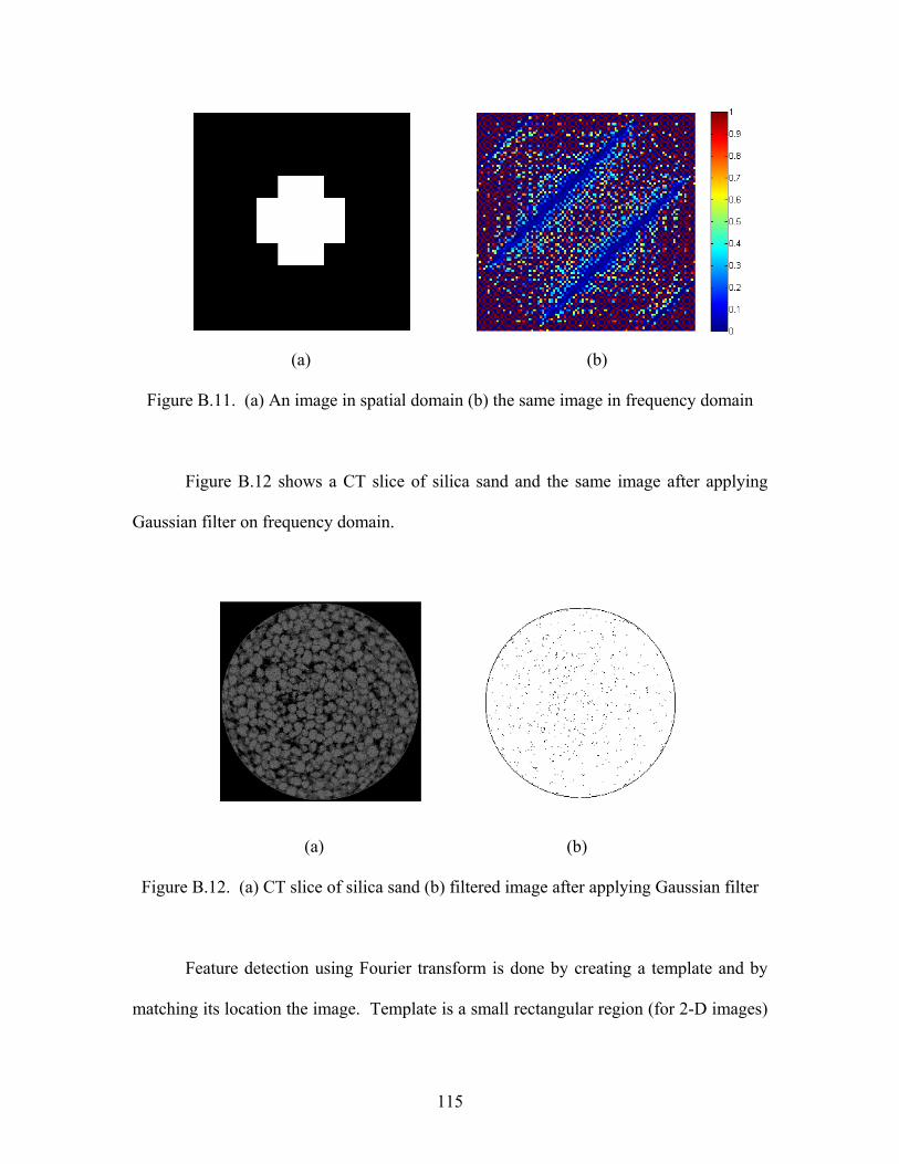
(a) (b)
Figure B.11. (a) An image in spatial domain (b) the same image in frequency domain
Figure B.12 shows a CT slice of silica sand and the same image after applying
Gaussian filter on frequency domain.
(a) (b)
Figure B.12. (a) CT slice of silica sand (b) filtered image after applying Gaussian filter
Feature detection using Fourier transform is done by creating a template and by
matching its location the image. Template is a small rectangular region (for 2-D images)
115

or a box volume (for 3-D images) of the image, which contains the desired feature. The
correlation of the template with the original image is computed and the maximum pixel
values identify the locations of the template.
Figure B.13 shows an image of a text in both horizontal and vertical directions.
To find the locations of letter “e” in horizontal direction, first a part of image containing
letter “e” is captured and stored as template (Figure B.14). Then the correlation of the
template with the original image is computed (Figure B.15). The maximum values of the
pixels on the correlated image correspond to the locations of the template in the image
(Figure B.16). Note that template must be rotated 90° clockwise before applying
correlation to find the template locations in the vertical text. For a general case the
rotation angle of the template is considered an unknown that is eventually found by
optimization.
Figure B.13. Image of a text
116

Figure B.14. Template image (magnified)
Figure B.15. Correlated image
117

Figure B.16. Locations of template in the image (white spots)
B.7.2 Discrete Cosine Transform (DCT)
The discrete cosine transform of a two dimensional image stored as a M×N matrix
A is defined by (MATLAB IPT 5.1):
∑ ∑−
=
−
=
++=
1
0
1
0 2)12(cos
2)12(cosM
m
N
n mnqppq Nqn
MpmAB ππαα
1010
−≤≤−≤≤
NqMp
(B.8)
αp and αq are defined by:
−≤≤
==
112
01
NqforN
qforNqα (B.9)
118

−≤≤
==
112
01
MpforM
pforMpα (B.10)
This transformation concentrates most of the visually significant information
about an image in a few coefficients. Therefore, this transformation is very useful for
image compression and it is used to compress the image using JPEG2 format. Discrete
cosine transformation is invertible and its inverse is given by:
∑ ∑−
=
−
=
++=
1
0
1
0 2)12(cos
2)12(cosM
p
N
q pqqpmn Nqn
MpmBA ππαα
1010
−≤≤−≤≤
NqMp
(B.11)
αp and αq are defined by:
−≤≤
==
112
01
NqforN
qforNqα (B.12)
−≤≤
==
112
01
MpforM
pforMpα (B.13)
Figure B.17 (a) shows a CT slice image in TIFF format and Figure B.17 (b)
shows that image after compression using discrete cosine transform. Though quality of
the compressed image is less, it is clearly recognizable and its size is 22.5 times less.
2 Joint Photographic Expert Group
119
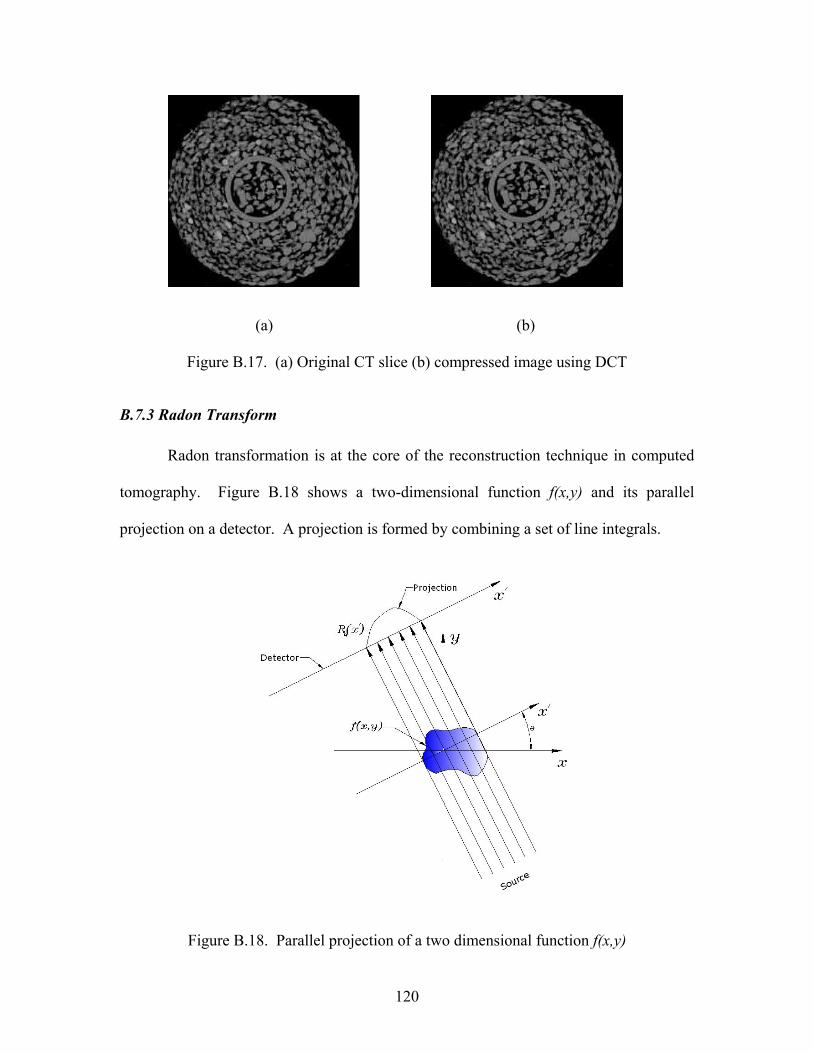
(a) (b)
Figure B.17. (a) Original CT slice (b) compressed image using DCT
B.7.3 Radon Transform
Radon transformation is at the core of the reconstruction technique in computed
tomography. Figure B.18 shows a two-dimensional function f(x,y) and its parallel
projection on a detector. A projection is formed by combining a set of line integrals.
Figure B.18. Parallel projection of a two dimensional function f(x,y)
120

If the distance of any point of f(x,y) from the origin along x′ axis is indicated by t,
then Radon transformation is given by (MATLAB IPT 5.1):
∫ ∫∞
∞−
∞
∞−
−+=ℜ dxdytyxyxfyxf )sincos(),()},({ θθδ (B.14)
δ is the Dirac delta function defined by:
≠=∞
=000
)(zifzif
zδ (B.15)
If the source is placed in a fixed position relative to line of detector another type of
projection is formed, which is known as a fan beam projection (Figure B.19).
Figure B.19. Fan beam projection of a two dimensional function f(x,y)
121

For two dimensional images with parallel projection, Radon transformation at
each point along the detector line (x′ ) is simply determined by adding all the pixel values
along the ray perpendicular to the point. Figures B.20, and B.21 show Radon transform
of a cross-shaped logical image at 0° and 45° angles, respectively. The horizontal axis
shows the pixels along the projection line and vertical axis shows the summation of the
pixels along each ray or the value of Radon transformation.
Figure B.20. Radon transform of a logical image at 0°
122

Figure B.21. Radon transform of a logical image at 45°
Radon transform is invertible and it can be used to reconstruct an image from its
projections at different angles. Figure B.22 shows 360 parallel projections of an image in
1° increment. Figure B.23 shows the reconstructed image from those projections using
inverse of Radon transform. Quality of the reconstructed image is a function of
projections. However, number of projections has an optimum more than which does not
have any effect on quality of the reconstructed image. Figures B.24 and B.25 show the
reconstructed images using 36 and 3600 projections, respectively. As it is seen 36
projections are not enough, while 3600 projections do not have any significant effect in
123

improving image quality. However, it is important to know that all reconstructed images
are subjected to some kinds of artifacts.
Figure B.22. 360 parallel projections of an image in 1° increment
124
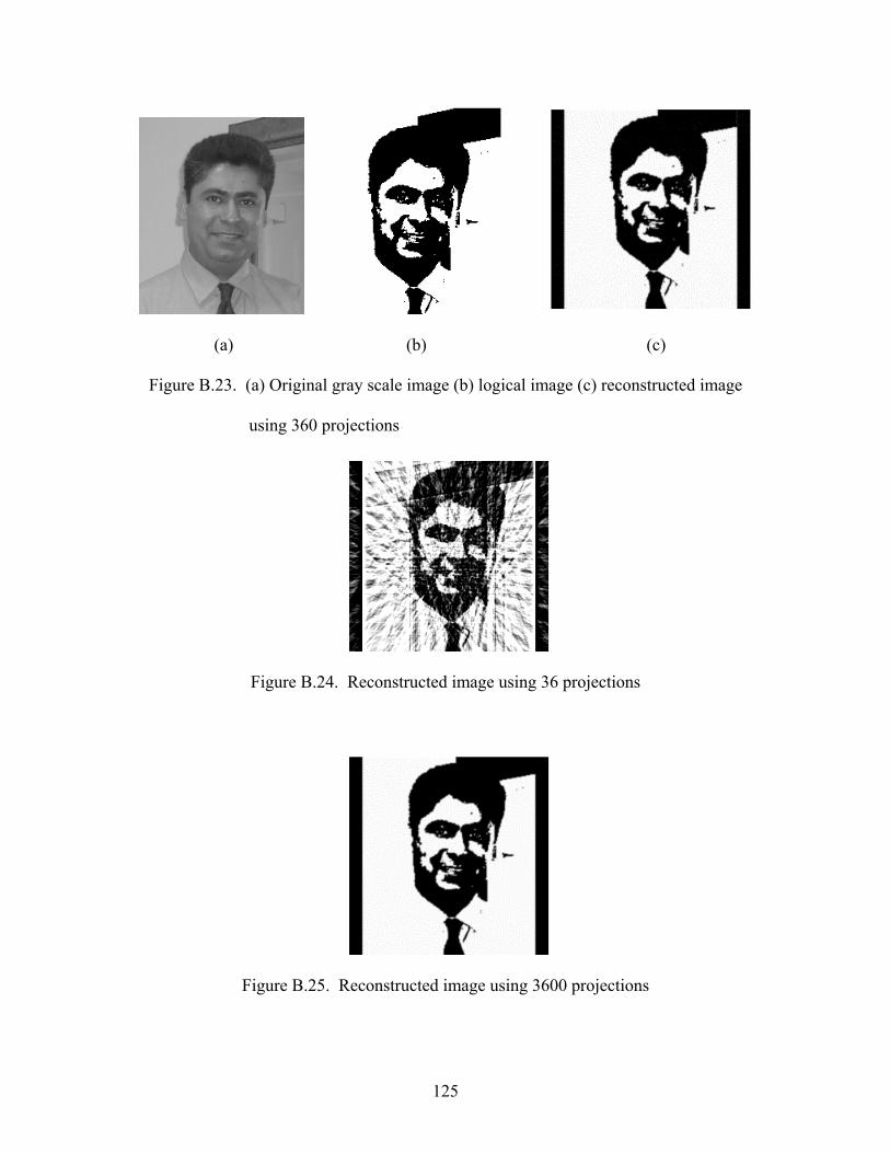
(a) (b) (c)
Figure B.23. (a) Original gray scale image (b) logical image (c) reconstructed image
using 360 projections
Figure B.24. Reconstructed image using 36 projections
Figure B.25. Reconstructed image using 3600 projections
125

B.8 Morphological Operations
Morphological operations are those that relate to shapes such as skeletonization,
filling, and segmentation. Skeletonization reduces all objects in an image to lines
according to image structure (Figure B.26). Filling is a morphological reconstruction
operation used to fill the closed loops (Figure B.27). Segmentation subdivides an image
into objects. It is considered to be one of the most difficult tasks in image processing.
Several methods exists for segmentation and we present a brief description of the
watershed transform (Gonzalez et al. 2004).
(a) (b)
Figure B.26. (a) Original image (b) image after skeletonization
126

(a) (b)
Figure B.27. (a) Original image (b) image after filling holes (closed loops)
B.9 Watershed Transform
Merriam-Webster’s Collegiate Dictionary (2006) defines watershed as a “divide”
or “a region or area bounded peripherally by a divide and draining ultimately to a
particular water course or body of water”. The same concept is used in image processing
to solve variety of image segmentation problems. If the gray scale vales on the images
are considered as elevations on a topography map then the dividing lines between humps
or pits are known as watershed lines or watershed ridge lines. Figure B.29 shows a gray
scale image of four circles. For the two top circles gray shades varies from 0 at the center
to 255 around the edges, while for the two bottom circles gray shades varies from 0
around the edges to 255 at the center. Figure B.30 is a representation of these circles in a
3-D Euclidian space by assuming an elevation equal to the gray shade value of each
pixel.
127

Figure B.28. A gray scale image of four circles touching two by two
It is evident that the circles form two humps and two pits. The dividing lines between the
two humps or the two pits are called watershed lines. Watershed segmentation is a very
useful operation in the segmentation of granular material images.
128

Figure B.29. Representation of circles in Figure B.29 assuming an elevation of gray
shade values at each pixel
One of the commonly used tool in conjunction with watershed transform for
segmentation is the distance transform. It is the distance from every pixel to the nearest
nonzero-valued pixel in a logical image. The distance transforms of one-valued pixels
are zero. A practical application of watershed transform in segmentation of touching
glass beads is shown in Figure B.30.
129
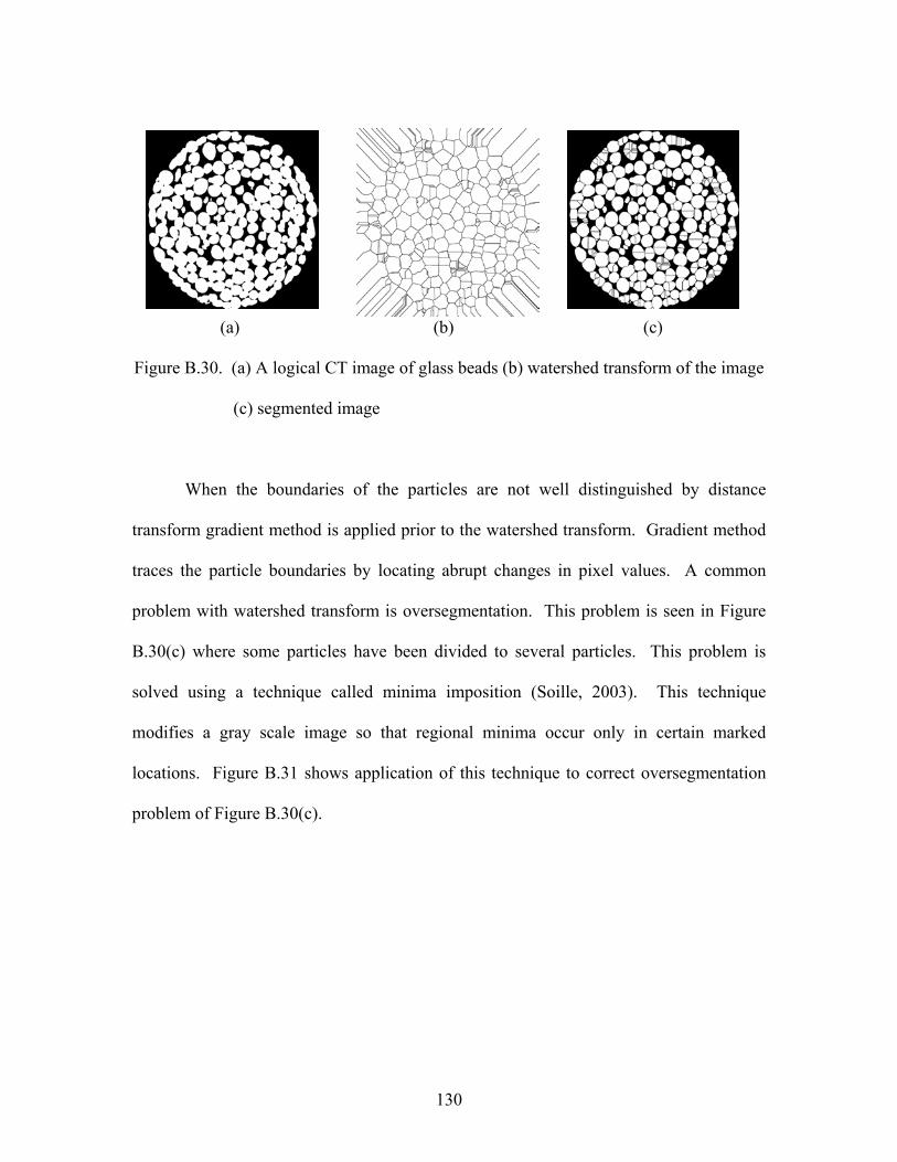
(a) (b) (c)
Figure B.30. (a) A logical CT image of glass beads (b) watershed transform of the image
(c) segmented image
When the boundaries of the particles are not well distinguished by distance
transform gradient method is applied prior to the watershed transform. Gradient method
traces the particle boundaries by locating abrupt changes in pixel values. A common
problem with watershed transform is oversegmentation. This problem is seen in Figure
B.30(c) where some particles have been divided to several particles. This problem is
solved using a technique called minima imposition (Soille, 2003). This technique
modifies a gray scale image so that regional minima occur only in certain marked
locations. Figure B.31 shows application of this technique to correct oversegmentation
problem of Figure B.30(c).
130

Figure B.31. Correction of oversegmentation problem in Figure B.31(c) using minima
imposition technique
131

Appendix C
AN ALTERNATE DESIGN OF X-RAY CT TRIAXIAL
If the required axial load or cell pressure is more than the maximum values in the
first design, then a different approach must be employed. It is evident that in this case a
large and heavy loading frame is required, which can not be mounted on the top of the
cell. Figure C.1 shows a section of the loading frame and the cell. Loading frame is
placed outside imaging area, and cell is designed for a tensile hoop stress only. Top cap
and base plate of the cell are connected using a few steel rods out of the imaging area. In
this design position of the loading frame is fixed, while cell, specimen, and loading ram
rotate with the rotation of the X-ray CT stage. In this case two ball-bearing systems are
used to reduce the friction, one on the top, and the other at the bottom of the cell.
This design guarantees application of very large loads and cell pressures inside
the X-ray CT chamber, unless the stage motor cannot provide adequate torque for
rotation. This design is applicable for both compressive and tensile triaxial test on a wide
range of materials including asphalt concrete, concrete, metals, rocks, etc.
132
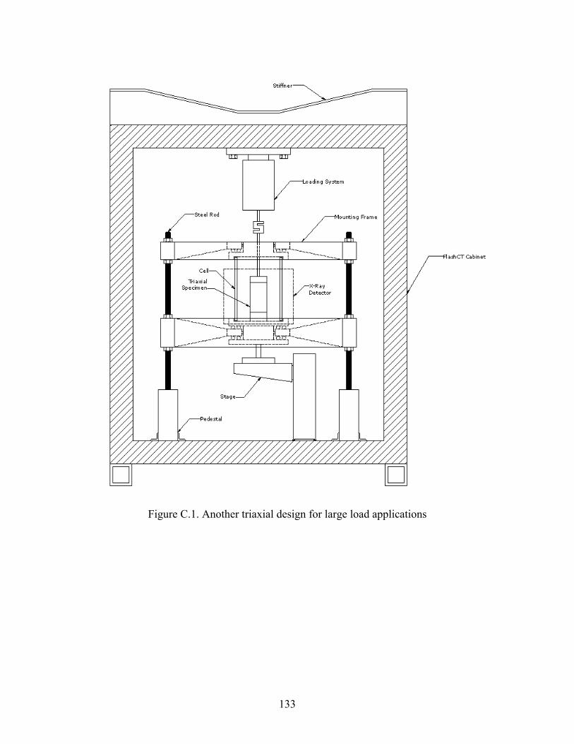
Figure C.1. Another triaxial design for large load applications
133