Mist and microstructure characterization in end milling ...
143
APPROVED: Nourredine Boubekri, Major Professor Thomas W. Scharf, Co-Major Professor Rajarshi Banerjee, Committee Member Peter Collins, Committee Member Marcus Young, Committee Member Narendra Dahotre, Chair of the Department of Materials Science and Engineering Costas Tsatsoulis, Dean of the College of Engineering Mark Wardell, Dean of the Toulouse Graduate School MIST AND MICROSTRUCTURE CHARACTERIZATION IN END MILLING AISI 1018 STEEL USING MICROLUBRICATION Vasim Shaikh, B.E., M.S Dissertation Prepared for the Degree of DOCTOR OF PHILOSOPHY UNIVERSITY OF NORTH TEXAS August 2013
Transcript of Mist and microstructure characterization in end milling ...

APPROVED: Nourredine Boubekri, Major Professor Thomas W. Scharf, Co-Major Professor Rajarshi Banerjee, Committee Member Peter Collins, Committee Member Marcus Young, Committee Member Narendra Dahotre, Chair of the Department of
Materials Science and Engineering Costas Tsatsoulis, Dean of the College of
Engineering Mark Wardell, Dean of the Toulouse Graduate
School
MIST AND MICROSTRUCTURE CHARACTERIZATION IN END MILLING AISI 1018
STEEL USING MICROLUBRICATION
Vasim Shaikh, B.E., M.S
Dissertation Prepared for the Degree of
DOCTOR OF PHILOSOPHY
UNIVERSITY OF NORTH TEXAS
August 2013
Shaikh, Vasim. Mist and microstructure characterization in end milling AISI 1018 steel
using microlubrication. Doctor of Philosophy (Materials Science and Engineering), August 2013,
129 pp., 90 illustrations, references, 90 titles.
Flood cooling is primarily used to cool and lubricate the cutting tool and workpiece
interface during a machining process. But the adverse health effects caused by the use of flood
coolants are drawing manufacturers’ attention to develop methods for controlling occupational
exposure to cutting fluids. Microlubrication serves as an alternative to flood cooling by reducing
the volume of cutting fluid used in the machining process. Microlubrication minimizes the
exposure of metal working fluids to the machining operators leading to an economical, safer and
healthy workplace environment. In this dissertation, a vegetable based lubricant is used to
conduct mist, microstructure and wear analyses during end milling AISI 1018 steel using
microlubrication. A two-flute solid carbide cutting tool was used with varying cutting speed and
feed rate levels with a constant depth of cut. A full factorial experiment with Multivariate
Analysis of Variance (MANOVA) was conducted and regression models were generated along
with parameter optimization for the flank wear, aerosol mass concentration and the aerosol
particle size. MANOVA indicated that the speed and feed variables main effects are significant,
but the interaction of (speed*feed) was not significant at 95% confidence level. The model was
able to predict 69.44%, 68.06% and 42.90% of the variation in the data for both the flank wear
side 1 and 2 and aerosol mass concentration, respectively. An adequate signal-to-noise precision
ratio more than 4 was obtained for the models, indicating adequate signal to use the model as a
predictor for both the flank wear sides and aerosol mass concentration. The highest average mass
concentration of 8.32 mg/m3 was realized using cutting speed of 80 Surface feet per minute
(SFM) and a feed rate of 0.003 Inches per tooth (IPT). The lowest average mass concentration of
5.91 mg/m3 was realized using treatment 120 SFM and 0.005 IPT. The cutting performance
under microlubrication is five times better in terms of tool life and two times better in terms of
materials removal volume under low cutting speed and feed rate combination as compared to
high cutting speed and feed rate combination. Abrasion was the dominant wear mechanism for
all the cutting tools under consideration. Other than abrasion, sliding adhesive wear of the
workpiece materials was also observed. The scanning electron microscope investigation of the
used cutting tools revealed micro-fatigue cracks, welded micro-chips and unusual built-up edges
on the cutting tools flank and rake side. Higher tool life was observed in the lowest cutting speed
and feed rate combination. Transmission electron microscopy analysis at failure for the treatment
120 SFM and 0.005 IPT helped to quantify the dislocation densities. Electron backscatter
diffraction (EBSD) identified 4 to 8 µm grain size growth on the machined surface due to
residual stresses that are the driving force for the grain boundaries motion to reduce its overall
energy resulting in the slight grain growth. EBSD also showed that (001) textured ferrite grains
before machining exhibited randomly orientated grains after machining. The study shows that
with a proper selection of the cutting parameters, it is possible to obtain higher tool life in end
milling under microlubrication. But more scientific studies are needed to lower the mass
concentration of the aerosol particles, below the recommended value of 5 mg/m3 established by
Occupational Safety and Health Administration (OSHA).

Copyright 2013
by
Vasim Shaikh
ii

ACKNOWLEDGEMENTS
I would like to express my sincere and deepest gratitude to my advisor, Dr. Nourredine
Boubekri, for his invaluable guidance, support and mentorship for this study and throughout my
course of study for the masters and Ph.D. program at the University of North Texas. His
guidance and inspiration enabled me to successfully complete my dissertation. I feel honored to
have had the opportunity to work under his supervision.
I would also like to thank my co-advisor Dr. Thomas W. Scharf, for his suggestions and
mentorship without which this study would not have been possible. I am grateful for his
helpfulness, cooperation and willingness to answer questions anytime.
I appreciate the kindness of Drs. Rajarshi Banerjee, Peter Collins and Marcus Young for
serving on my dissertation committee. Their contributions and suggestions helped to improve
this work tremendously. I thank them for giving their valuable time to guide me and review my
dissertation. I would also like to appreciate the selfless and generous help of Dr. Junyeon Hwang,
Dr. Hamidreza Mohseni, Jon-Erik Mogonye, Douglas Kinkenon, Peyman Samimi, David Brice
and Victor Ageh. I would also like to acknowledge the Center for Advanced Research and
Technology (CART) and the Manufacturing Engineering Laboratory at the University of North
Texas.
I am, as ever, indebted to my parents Mrs. and Mr. Abdul Majid Shaikh for their love and
support throughout my life. I would not have come this far without the understanding and
support of my wife, Firoza Khan. I thank her from the bottom of my heart to help me achieve my
goals.
iii

TABLE OF CONTENTS
Page
ACKNOWLEDGEMENTS...........................................................................................................iii
LISTS OF TABLES......................................................................................................................vii
LISTS OF FIGURES...................................................................................................................viii
Chapters
1. INTRODUCTION ..................................................................................................1
Background .................................................................................................1
Microlubrication ........................................................................................ 4
Multivariate Analysis of Variance (MANOVA) ........................................6
Why Use MANOVA ...................................................................................7
Research Objective ....................................................................................7
2. LITERATURE REVIEW .......................................................................................9
Microlubrication Drilling ............................................................................9
Microlubrication Milling Other than Steel ...............................................13
Microlubrication End Milling Steel ..........................................................18
Fluids not Suggested for Microlubrication ...............................................26
Why Use Vegetable Oil ............................................................................26
Why Use AISI 1018 Steel .........................................................................27
Summary ...................................................................................................28
Conclusion ................................................................................................28
3. EXPERIMENTAL METHODS AND PROCEDURES ......................................30
Design of Experiments ..............................................................................30
iv

Cutting Tool ..............................................................................................31
Workpiece Material ..................................................................................32
End milling equipment .............................................................................36
Metal Working Fluid (MWF) ...................................................................37
Aerosol Mass Concentration and Aerosol Particle Size Measurements ...38
Samples Preparation ..................................................................................39
End Milling Procedures ............................................................................40
Method of Data Analysis for MANOVA ..................................................42
MANOVA Assumptions ...........................................................................42
Robustness of MANOVA .........................................................................43
Hypotheses ................................................................................................44
Tool Flank Wear Measurements ...............................................................44
Tool-Workpiece Interface Temperature Calculations ..............................46
Vickers Hardness Measurement ...............................................................49
Bearing Area Curve Measurement ...........................................................52
Scanning Electron Microscopy (SEM) / Focused Ion Beam (FIB) ..........53
Electron Backscatter Diffraction (EBSD) ................................................54
Transmission Electron Microscopy (TEM) ..............................................54
Dislocation Density Quantification Procedure .........................................55
Assumptions of the Study .........................................................................58
4. RESULTS AND ANALYSES .............................................................................59
MANOVA .................................................................................................59
Aerosol Mass Concentration and Aerosol Particle Size Analysis ............79
v

Tool-Workpiece Interface Temperature Analysis ....................................80
Tool Life ...................................................................................................85
Wear Mechanisms ....................................................................................87
Cross Sectional Hardness Analysis at Failure ..........................................95
Bearing Area Curve Calculations .............................................................96
TEM Analysis at Failure .........................................................................100
EBSD Analysis .......................................................................................108
5. SUMMARY AND CONCLUSIONS .................................................................118
Recommendations for Future Work ........................................................122
REFERENCES ...........................................................................................................................123
vi

LIST OF TABLES
Page
1. Permissible exposure limits (PELs) ....................................................................................3
2. Factorial experiment layout of cutting speed and feed rate combinations ........................30
3. Chemical composition of AISI 1018 steel ........................................................................33
4. Mechanical properties of AISI 1018 steel ........................................................................33
5. Mechanical properties of Accu-Lube 6000 .......................................................................38
6. Average and maximum flash temperature formulae for line contacts ..............................48
7. MANOVA test summarized results ..................................................................................67
8. ANOVA test for flank wear side 1 ...................................................................................68
9. ANOVA test for flank wear side 2 ...................................................................................68
10. ANOVA test for aerosol mass concentration ....................................................................68
11. ANOVA test for aerosol particle size ...............................................................................68
12. Temperature calculations for different cutting speed and feed rate combinations ...........84
13. Roughness parameter for different cutting speed and feed rate combinations ...............100
14. CBED data for thickness determination .........................................................................104
vii

LISTS OF FIGURES
Page
1. External spray MQL system ...............................................................................................5
2. Solid carbide end mill .......................................................................................................32
3. Schematic representation of microstructures for AISI 1018 steel ....................................34
4. SEM image of as-received AISI 1018 steel ......................................................................35
5. TEM image of pearlite ......................................................................................................35
6. Mori Seiki Dura Vertical 5060 machining center .............................................................36
7. Kuroda ecosaver KEP3 micro lubrication system ............................................................37
8. Thermo scientific DataRam4 ............................................................................................39
9. Final sample ......................................................................................................................40
10. Mitutoyo toolmaker’s microscope ....................................................................................45
11. Optical micrograph of tool rake side 1 - Treatment 100 SFM and 0.003 IPT ..................46
12. Shimadzu dynamic ultra micro hardness tester ................................................................50
13. Schematic of vickers hardness measurements ..................................................................51
14. Bakelite mount ..................................................................................................................51
15. Nanovea non-contact optical profilometer ........................................................................52
16. Dual beam Nova 200 NanoLab SEM/FIB ........................................................................53
17. (a) Tecnai G2 F20 TEM ....................................................................................................55
17. (b) Necessary measurements to extract thickness (t) from K-M fringes ..........................56
18. Test for equal covariance for flank wear side 1 ................................................................60
19. Test for equal covariance for flank wear side 2 ................................................................60
viii

20. Test of equal covariance for aerosol mass concentration .................................................61
21. Test for equal covariance for aerosol particle size ............................................................61
22. Constant variance in data for flank wear side 1 ................................................................62
23. Constant variance in data for flank wear Side 2 ...............................................................62
24. Constant variance in data for aerosol mass concentration ................................................63
25. Constant variance in data for aerosol particle size ............................................................63
26. Mahalanobis distance for multivariate normality testing for flank wear side 1, side 2, aerosol mass concentration and aerosol particle size ........................................................64
27. Normal plots of residual in data for flank wear side 1 ......................................................65
28. Normal plots of residual in data for flank wear side 2 ......................................................66
29. Normal plots of residual in data for aerosol mass concentration ......................................66
30. Normal plots of residual in data for aerosol particle size .................................................67
31. Down-milling (Climb milling) and Up-milling (Conventional milling) ..........................70
32. Main effect plot for flank wear side 1 ..............................................................................72
33. Interaction plot for flank wear side 1 ................................................................................72
34. Main effect plot for flank wear side 2 ...............................................................................73
35. Interaction plot for flank wear side 2 ................................................................................73
36. Tool run-out ......................................................................................................................74
37. Main effect plot for aerosol mass concentration ..............................................................74
38. Interaction plot for aerosol mass concentration ................................................................75
39. Desirability plot for flank wear side 1 ..............................................................................76
40. Selected solution plot for flank wear side 1 .....................................................................76
41. Desirability plot for flank wear side 2 ..............................................................................77
42. Selected solution plot for flank wear side 2 .....................................................................77
ix
43. Desirability plot for aerosol mass concentration ..............................................................78
44. Selected solution plot for aerosol mass concentration .....................................................78
45. Average mass concentration for different cutting speeds and feed rates combinations ...79
46. Average particle size for different cutting speeds and feed rates combinations ...............80
47. Tool life for different cutting speeds and feed rates combinations at failure ...................85
48. Material removal volume for different cutting speeds and feed rates combinations at failure.................................................................................................................................86
49. Optical micrograph of tool flank wear for treatment (a) 80 SFM and 0.003 IPT (b) 120 SFM and 0.003 IPT (c) 100 SFM and 0.005 IPT (d) 120 SFM and 0.005 IPT (e) 100 SFM and 0.003 IPT ....................................................................................................................87
50. Optical micrograph of tool rake for treatment 100 SFM and 0.003 IPT ..........................88
51. Optical micrograph of tool rake for treatment 80 SFM and 0.005 IPT ............................89
52. SEM micrograph of tool rake for treatment 120 SFM and 0.005 IPT showing sliding wear ............................................................................................................................................89
53. SEM micrograph of tool rake for treatment 120 SFM and 0.005 IPT showing non-uniform micro-abrasion (a) Rake (b) Flank ......................................................................90
54. SEM micrograph of tool flank for treatment 80 SFM and 0.003 IPT showing micro-
fatigue crack ......................................................................................................................91 55. SEM micrograph of tool for treatment 120 SFM and 0.005 IPT showing welded micro-
chips (a) Rake (b) Flank ....................................................................................................91 56. SEM micrograph of tool rake for treatment 80 SFM and 0.003 IPT showing sliding wear
............................................................................................................................................92 57. SEM micrograph of tool for treatment 80 SFM and 0.003 IPT showing non-uniform
micro-abrasion (a) Rake (b) Flank ....................................................................................93 58. SEM micrograph of tool flank for treatment 80 SFM and 0.003 IPT showing adhesion .93
59. SEM micrograph of tool rake for treatment 80 SFM and 0.003 IPT showing adhesion and built-up edge (BUE) .........................................................................................................94
60. SEM micrograph of workpiece for treatment 80 SFM and 0.003 IPT showing abrasive wear through plowing mechanism ....................................................................................95
x

61. Microhardness depth profile of cross-section for treatment 120 SFM and 0.005 IPT .....96
62. Microhardness depth profile of cross-section for treatment 80 SFM and 0.003 IPT .......96
63. Surface profile at failure for treatment 120 SFM and 0.005 IPT ......................................97
64. Surface profile at failure for treatment 80 SFM and 0.003 IPT ........................................97
65. Histogram for treatment 120 SFM and 0.005 IPT ............................................................98
66. Histogram for treatment 80 SFM and 0.003 IPT ..............................................................98
67. Bearing area curve at failure for treatment 120 SFM and 0.005 IPT ...............................99
68. Bearing area curve at failure for treatment 80 SFM and 0.003 IPT .................................99
69. Lift-out area 20µm from machined edge for treatment 120 SFM and 0.005 IPT ..........101
70. TEM image showing dislocations for a depth of 20 µm from machined edge for treatment 120 SFM and 0.005 IPT ..................................................................................................102
71. (a) and (b) TEM image showing dislocation pile-ups for a depth of 20 µm from machined edge for treatment 120 SFM and 0.005 IPT ...................................................................103
72. TEM image showing fewer dislocations for a depth of 100 µm from machined edge for
treatment 120 SFM and 0.005 IPT ..................................................................................103
73. Intercept plot to extrapolate foil thickness value ............................................................104
74. (a) TEM micrograph of image 1 used to determine ρ by the line intersection method at a depth of 20 µm from machined edge for treatment 120 SFM and 0.005 IPT ................105
74. (b) TEM micrograph of image 2 used to determine ρ by the line intersection method at a
depth of 20 µm from machined edge for treatment 120 SFM and 0.005 IPT ................106 75. Dislocation density quantification at a depth of 20 µm from machined edge for treatment
120 SFM and 0.005 IPT ..................................................................................................106
76. IPF for all phases – As received material .......................................................................109
77. IPF for ferrite and iron carbide phase – As received material ........................................109
78. IPF for all phases – Sample 1 and 2 machined at 80 SFM and 0.003 IPT .....................110
79. IPF for ferrite phase – Sample 1 and 2 machined at 80 SFM and 0.003 IPT .................110
xi

80. IPF for iron carbide phase – Sample 1 and 2 machined at 80 SFM and 0.003 IPT ........111
81. IPF for all phases – Sample 1 and 2 machined at 120 SFM and 0.005 IPT ...................111
82. IPF for ferrite phase – Sample 1 and 2 machined at 120 SFM and 0.005 IPT ...............112
83. IPF for iron carbide phase – Sample 1 and 2 machined at 120 SFM and 0.005 IPT ......112
84. Grain size comparison .....................................................................................................113
85. Grain size distribution plot – As- received material .......................................................114
86. Grain size distribution plot for 80 SFM and 0.003 IPT – Sample 1 ...............................115
87. Grain size distribution plot for 120 SFM and 0.005 IPT – Sample 1 .............................115
88. Ferrite pole figures – As received material .....................................................................116
89. Ferrite pole figures – Sample 1 and 2 machined at 80 SFM and 0.003 IPT ...................117
90. Ferrite pole figures – Sample 1 and 2 machined at 120 SFM and 0.005 IPT..................117
xii

CHAPTER 1
INTRODUCTION
Background
Metal cutting processes have been in practice for many centuries. The process of
machining any material is very complicated. It is dependent on many important factors such as
the machine tool, the machining conditions, the workpiece materials, the tool material, tool wear
and metal working fluid (MWF). Among these the most important controllable factor is the
MWF. MWFs are used to cool and lubricate the tool-workpiece interface during machining.
MWFs perform several important functions including reducing the friction-heat generation and
dissipating generated heat at the tool-workpiece interface which results in the reduction of tool
wear. MWFs increase tool life and achieve faster production rates (Clarens et al. 2008). Also,
MWFs flush the chips away from the tool and clean the workpiece causing less built-up-edge
(BUE). The first appearance of metal cutting fluid in the literature occurred in the mid-19th
century (Northcott, 1868). A more comprehensive work on cutting fluids was reported by F. W.
Taylor (Taylor, 1906). Since then, metal cutting fluids or MWFs have been used during metal
cutting.
The use of MWFs cannot be completely stopped because of their beneficial contributions.
But, the metal cutting industry wants to find ways to reduce/eliminate the usage of MWFs; the
use of MWFs in machining is thought to be undesirable for economical, health, and
environmental reasons. The cost incurred on MWFs range from 7-17% of the total costs of the
manufactured work piece (Weinert et al. 2004) and 16-20% of the total product cost (Sreejith &
Ngoi, 2000) as compared to the tool cost which is only about 2-4% (Zhang et al. 2012).
According to a survey conducted by the European Automobile Industry, the cost incurred by
1

lubricants comprises nearly 20% of the total manufacturing cost contrasted with the cost of the
cutting tool which is only 7.5% of the total cost (Brockhoff & Walter, 1998). More than 100
million gallons of MWFs are used in the Unites States of America each year and approximately
1.2 million employees are exposed to them and to their potential occupational health hazards
(Chalmers, 1999). According to the Federal Office of Economics, more than 78,800 tons of
cutting fluids was used in Germany in the year 2002 (Heisel et al. 2009). MWFs in the form of
airborne particles often remain suspended in the working environment for an extended period of
time and can be inhaled by the workers causing health concerns (Sutherland et al. 2000). U.S.
National Institute for Occupational Safety and Health (NIOSH) recommends that the exposure
limits (RELs) to MWF aerosols cannot exceed 0.5 mg/m3 total particulate mass as a time
weighted average (TWA) concentration for up to 10 hours per day during a 40 hours work week
(NIOSH, 1998) and cannot exceed 10 mg/m3 as a 15 minutes TWA short-term exposure limit
(STEL) (Park, 2012). The Occupational Safety and Health Administration (OSHA) have
currently two permissible exposure limits (PELs) applied to MWFs. They are 5 mg/m3 for an 8
hours TWA for mineral oil mist and 15 mg/m3 for an 8 hours TWA for particulates not otherwise
classified (PNOC) (Sheehan, 1999). The American Conference of Governmental Hygienists
(ACGIH) threshold limit value (TLV) and Health Safety Executive, UK, occupational exposure
limits (OELs) for mineral oils mist is 5 mg/m3 for an 8 hours TWA, and 10 mg/m3 for a 15
minutes STEL (Park, 2012). The Swiss recommendations for PELs is 0.2 mg/m3 for heavy oil
with boiling point greater than 350°C of aerosol and/or 20 mg/m3 of oil aerosol plus vapor for
medium or light oil. The German Institute of Occupational Health (BGIA) standard is 10 mg/m3
of oil aerosol plus vapor. In France, the National Institute for Research and Safety (INRS)
proposes a recommended value of 1 mg/m3 of aerosol (Huynh et al. 2009).
2
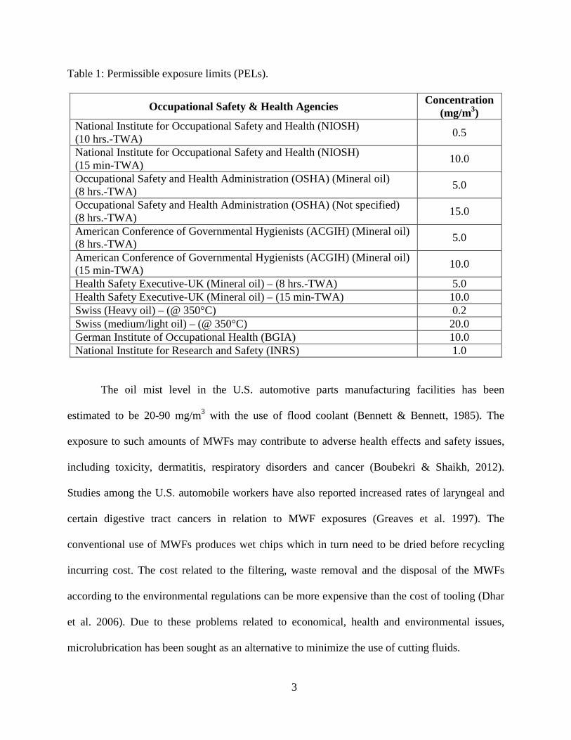
Table 1: Permissible exposure limits (PELs).
Occupational Safety & Health Agencies Concentration (mg/m3)
National Institute for Occupational Safety and Health (NIOSH) (10 hrs.-TWA) 0.5
National Institute for Occupational Safety and Health (NIOSH) (15 min-TWA) 10.0
Occupational Safety and Health Administration (OSHA) (Mineral oil) (8 hrs.-TWA) 5.0
Occupational Safety and Health Administration (OSHA) (Not specified) (8 hrs.-TWA) 15.0
American Conference of Governmental Hygienists (ACGIH) (Mineral oil) (8 hrs.-TWA) 5.0
American Conference of Governmental Hygienists (ACGIH) (Mineral oil) (15 min-TWA) 10.0
Health Safety Executive-UK (Mineral oil) – (8 hrs.-TWA) 5.0 Health Safety Executive-UK (Mineral oil) – (15 min-TWA) 10.0 Swiss (Heavy oil) – (@ 350°C) 0.2 Swiss (medium/light oil) – (@ 350°C) 20.0 German Institute of Occupational Health (BGIA) 10.0 National Institute for Research and Safety (INRS) 1.0
The oil mist level in the U.S. automotive parts manufacturing facilities has been
estimated to be 20-90 mg/m3 with the use of flood coolant (Bennett & Bennett, 1985). The
exposure to such amounts of MWFs may contribute to adverse health effects and safety issues,
including toxicity, dermatitis, respiratory disorders and cancer (Boubekri & Shaikh, 2012).
Studies among the U.S. automobile workers have also reported increased rates of laryngeal and
certain digestive tract cancers in relation to MWF exposures (Greaves et al. 1997). The
conventional use of MWFs produces wet chips which in turn need to be dried before recycling
incurring cost. The cost related to the filtering, waste removal and the disposal of the MWFs
according to the environmental regulations can be more expensive than the cost of tooling (Dhar
et al. 2006). Due to these problems related to economical, health and environmental issues,
microlubrication has been sought as an alternative to minimize the use of cutting fluids.
3

Microlubrication
Microlubrication is also known as green machining, minimum quantity lubrication
(MQL), near-dry machining, semi-dry machining or spatter lubrication. Microlubrication was
introduced by Horkos Corporation - Japan in 1992. Microlubrication consists of atomizing a very
small quantity of MWF ranging between 2 to 200 ml/hr directed toward the cutting
tool/workpiece interface in the form of an aerosol. In microlubrication technique, the MWF does
not recirculate through the lubrication system. It is almost all evaporated at the point of
application. Hence no recirculation is required. It is important however to ensure an efficient
extraction of aerosol from the machine. In microlubrication, the lubrication is obtained via the
MWF, and the cooling is achieved by pressurized air that reaches the cutting tool/workpiece
interface. Investigations have shown that microlubrication is effective at reducing cutting
tool/workpiece interface temperature, tool wear, thermal distortion and material adhesion to the
tool. In some studies using microlubrication the performance was equivalent to or better than
flood cooling (Kurgin et al. 2011).
There are two basic types of MQL systems: external spray MQL and through-tool MQL.
The external spray MQL system consists of a coolant tank or reservoir which is connected with
tubes fitted with one or more nozzles directed towards the tool/workpiece interface. As shown in
figure 1, the system has an independent adjustable air and coolant flow control knob which helps
to vary the coolant delivery.
4

Figure 1: External spray MQL system.
There are two basic types of through-tool MQL systems, based on a method of creating
an air-oil mist. The first is the external mixing or one-channel system. In this type, the oil and air
are mixed externally, and piped through the spindle and tool to the cutting zone. The second
technique is the internal mixing or two channel system. In this type, two parallel tubes are routed
through the spindle to bring oil and air to an external mixing device near the tool holder where
the mist is created (Filipovic & Stephenson, 2006).
The aerosol during microlubrication can be produced by two mechanisms: atomization
and vaporization/condensation. In atomization, aerosol is produced by the disintegration of
lubricant jet by the kinetic energy of the lubricant itself, by exposure to high velocity air or as a
result of mechanical energy applied externally through a rotating or vibrating device (Adler et al.
2006). Vaporization is produced as a result of heat generated at the tool/workpiece interface.
5
This heat is transferred to the lubricant and raises its temperature above the saturation
temperature resulting in boiling and vapor production at the workpiece/lubricant interface. This
vapor condenses spontaneously generating aerosol/mist (Sutherland et al. 2000). In regular
machining operations that use a flood coolant supply, cutting fluids have been selected mainly on
the basis of their characteristics, i.e., their cutting performance.
In microlubrication however, secondary characteristics of a lubricant are important, such
as their safety properties (environment pollution and human contact), biodegrability, oxidation
and storage stability. This is important because the lubricant must be compatible with the
environment and resistant to long term usage caused by low consumption (Wakabayashi et al.
2006). Further, microlubrication reduces induced thermal shock and helps to increase the
workpiece surface integrity in situations of high tool pressure (Attanasio et al. 2006).
Multivariate Analysis of Variance (MANOVA)
MANOVA is also known as multidimensional analysis of variance (Meyveci et al. 2011)
or multiple analysis of variance (Chakraborty, 2007). MANOVA is used to study the effects of
one or more independent variables on more than one dependent variable/s. MANOVA is a
conceptually straightforward extension of analysis of variance (ANOVA). The major distinction
is that in ANOVA one evaluates mean differences on a single dependent criterion variable,
whereas in MANOVA one evaluates mean differences of independent variables on two or more
dependent variables simultaneously (Bray & Maxwell, 1985; Hand & Taylor, 1987). MANOVA
is conducted in a two step process. The first step is to test the overall hypothesis of no
differences in the means for the different groups of independent variables. If this test is
significant, the second step is to conduct follow-up tests to explain the group differences if any.
6

Unlike ANOVA, there is not just one method (i.e. the F-test) to form a test statistics. Four
different tests may be employed in MANOVA; (i) Hotelling’s T-squared test (ii) Wilk’s lambda
(iii) Pillai-Bartlett test and (iv) Roy’s greatest character root (GCR) test. The Hotelling’s T-
squared test is a common traditional test used to compare the mean vectors of two groups formed
by the independent variables. The Wilk’s lambda test is conducted when there are more than two
groups formed by the independent variables. It is also one of the most common and widely used
traditional tests. The sum of explained variances of the discriminant variables are given by the
Pillai-Bartlett test (Bray & Maxwell, 1985).
Why Use MANOVA
Some of the reasons to use MANOVA in studies investigating mean differences are:
1. MANOVA helps us to evaluate the mean differences on all the dependent variables
simultaneously, rather than looking at each of them in isolation.
2. MANOVA gives us the opportunity to learn more about the data by looking at the
variables in some combination or pattern rather than looking at them individually.
3. MANOVA examines different dependent variables together, thus, it enhances the
interpretation of results and provides a more powerful test than doing separate ANOVAs.
Research Objectives
The primary objective of this research is to investigate the effectiveness of
microlubrication during end milling American Iron and Steel Institute (AISI) 1018 steel with a
solid carbide cutter under varying cutting speed and feed rate levels and a constant depth of cut
using Acculube 6000 vegetable based lubricant. A full factorial experiment and regression
7

models along with parameter optimization for the aerosol mass concentration, aerosol particle
size and tool flank wear are generated. Microstructure and mist characterizations are done for the
high cutting speed/high feed rate level and the low cutting speed/low feed rate level.
The following tasks are specifically addressed in the study:
1. Investigate the workpiece subsurface deformation.
2. Investigate the subsurface strengthening taken place due to the dislocation activities.
3. Investigate the effects of each independent variable (i.e. cutting speed and feed rate) on
aerosol mass concentration, aerosol particle size and tool flank wear.
4. Develop predicting models for aerosol mass concentration, aerosol particle size and tool
flank wear.
5. Investigate the correlation between all dependent variable (i.e. aerosol mass
concentration, aerosol particle size and tool flank wear).
6. Estimate the cutting zone temperature for all cutting conditions.
7. Examine the wear process and mechanisms on the tool flank and cause of tool failure.
8. Examine surface texture and grain size evolution before and after machining.
8

CHAPTER 2
LITERATURE REVIEW
Studies in microlubrication were largely initiated in 1992 by Horkos Corporation in
Japan. Since the last decade, microlubrication is realized to address issues pertaining to
economical benefits, occupational hazards and environmental pollution. Several materials have
been reported using microlubrication including carbon steels, alloy steels, aluminum, nodular
cast iron, inconel and titanium. In microlubrication, vegetable oil or synthetic ester oil are mainly
used as lubricant instead of mineral oil. Much research has been carried out to study the effects
of microlubrication during drilling, milling and turning operations. However, no research is
carried out in end milling American Iron and Steel Institute (AISI) 1018 steel using
microlubrication. The following section is organized with literature review related to
microlubrication with different machining operations.
Microlubrication Drilling
Experiments were carried out to evaluate the effectiveness of microlubrication in
achieving higher penetration rate when drilling 1038 steel. Two sets of thru-tool drilling
experiments were carried out at a penetration rate of 537 mm/min and 974 mm/min, respectively.
A vegetable oil metal working fluid (MWF) (Acculube 6000) was used as the lubricant with a
delivery rate of 50 ml/hr at an air pressure of 4.96 bars. Two solid carbide titanium aluminum
nitride (TiAlN) coated drills were used to drill 730 holes with a cutting speed of 80 m/min and a
feed rate of 0.13 mm/rev for the first set of experiment. Both the drills were analyzed before and
after drilling. There was minimal margin and flank wear. The maximum flank wear was 0.13 mm at
the outer corner. There was some minimal buildup of material on the margins and near the chisel
edge. The spindle power was observed to be constant with the hole depth. For the second set of
9

experiments, four new drills were used along with one reground and retested, with a cutting speed of
90 m/min and a feed rate of 0.2 mm/rev. The first drill broke on the first hole. The second drill
produced sparks and excessive noise after 15 holes due to chipping at the corner of the tool. The
third, fourth and the reground tool drilled more than 900 holes. Neither for these tools showed
excessive margin or flank wear, although the reground tool showed noticeable build up edge
behind the margin. It was concluded that microlubrication can be used for drilling at a much
higher penetration rates than gun drilling. Build-up edges (BUE) was observed on the margins
and the flanks may be due to excessive hole temperatures. BUE was more common on reground
drills than the new ones (Filipovic & Stephenson, 2006).
A study was conducted to report the optimum conditions for ecological deep hole drilling
(Murakami & Yamamoto, 2007). The drills having a diameter of 6 mm were specially coated
with TiAlN film and a polycrystalline diamond layer. A comparison was done using minimum
quantity lubrication (MQL) and emulsion coolant. The work materials used were
(S50C/SCM440/FCD700 and carbon steel S48C) to drill a 120 and 106 mm deep hole at a flow
rate of 10 cc/min using thru-tool lubrication. The cutting speed of 80 and 60 m/min were used
along with a constant feed rate of 0.2 mm/rev. It was observed that both the thrust force and
cutting torque obtained under MQL were lower than those under emulsion coolant. The drill life
obtained by MQL was 2 times longer than that by emulsion coolant. The carbon steel workpiece
was more easily cut by MQL than using emulsion because the workpiece was softened due to the
increase in temperature because the cutting was done without a large amount of coolant. The
outside nozzle lubrication was also carried out using MQL and emulsion coolant. The workpiece
material used was carbon steel S45C. The cutting speeds used were 50, 80, 120, 150 and 180
m/min. The feed rate used was 0.12 mm/min to drill an 18 mm deep hole. MQL was less
10
effective at high speeds. But, as many as 9283 holes were drilled using MQL at the cutting speed
of 120 m/min. While for all the cutting conditions using emulsion cooling, the maximum
numbers of holes drilled by were only 4500. It was concluded that MQL was able to lengthen the
tool life as compared to emulsion cutting (Murakami & Yamamoto, 2007).
In 2008, a research study was carried out for possible improvements in drilling 319 Al
using diamond-like carbon (DLC) coated high-speed steel (HSS) and uncoated HSS tools under
external nozzle MQL (Bhowmick & Alpas, 2008). Two types of DLCs (non-hydrogenated and
hydrogenated) were considered. The results were compared to drilling using conventional flood
coolant and dry drilling. Distilled water spray was used as a minimum quantity lubricant at a
flow rate of 30 ml/hr to drill 19 mm deep hole. For flood cooling, water-soluble coolant was used
at a flow rate of 30,000 ml/hr. The drilling tests were performed at a cutting speed of 50 m/min
using a feed rate of 0.25 mm/rev. It was observed that the torque and thrust force required by
MQL drilling were less as compared to dry drilling to a level similar to the performance under
the flood condition. In MQL drilling, the mass of Al that adhered to drill bits decreased
considerably compared to dry drilling. In addition, a more stable cutting condition was reached
as evidenced by the lower number of spikes (sudden jumps due to Al adhesion) in torque and
thrust force curves. It was also observed that the smallest BUE formation on the cutting edge of
the drill, as well as the Al adhesion to the drill flutes, occurred during MQL drilling with non-
hydrogenated DLC, concluding that this type of DLC coating is the preferred coating for drilling
316 Al using a minimum quantity of lubrication (Bhowmick & Alpas, 2008).
Dosbaeva et al. 2008 conducted a research study to improve and evaluate the through-
tool MQL conditions. Drills with DLC physically-vapor-deposited (PVD) coatings were again
coated with thin perfluoropolyether (PFPE) lubricant films and were compared to traditional
11

tooling used in wet-machining conditions for the drilling of a cast aluminum-silicon B319 alloy.
Approximately 1000 holes were drilled with two types of coatings (DLC; DLC + PFPE) and the
progression in flank wear rate, surface finish, tool life and cutting torque were compared. The
drilling tests were performed at a cutting speed of 94 m/min using a feed rate of 0.13 mm/rev to
drill a 19 mm deep hole. An improvement in the frictional properties of cutting tools prepared
with DLC + PFPE coatings was observed for MQL machining conditions. The PFPE surface
treatment was found to reduce the cutting torque as well as increase tool life and improve the
surface finish of the machined part (Dosbaeva et al. 2008).
In another study, burr analyses were carried out on the drilling process as a function of
tool wear and different lubricant-coolant condition (Costa et al. 2009). Dry drilling, use of MQL
at a flow rate of 30 ml/hr and fluid applied in conventional way (flood cooling) were compared.
The MWFs used were: vegetable oil Accu-Lube-LB-2000 as MQL, mineral oil Shell DMI 410 as
MQL and flood coolant, and semi-synthetic oil Shell DMS 250 EP as flood coolant. The trials
were carried out at two cutting speeds (45 and 60 m/min) to drill hole having length/diameter
(L/D) ratio of 3. The tool used in the tests was the solid twist HSS drill coated with TiAlN, with
diameter of 10 mm, to drill the microalloyed steel DIN 38MnS6. The criterion adopted for the
end of the test was the catastrophic failure of the drill. It was observed that the MQL system with
mineral oil produced the largest average burr heights, while the MQL system with vegetable oil
(Acculube LB-2000), along with the dry system, produced the smallest burr heights. The results
also showed that the height of the burr increases primarily with the wear of the tool and that this
increase is almost exponential after 64% and 84% of drills life, for the speeds of 45 and 60
m/min, respectively. Also, the dry machining tests caused a severe and sudden wear of the
12

cutting edges of the drill, in such a way that the drill lives were significantly inferior to those of
the other systems (Costa et al. 2009).
Shaikh & Boubekri, 2010 investigated the effectiveness of MQL in drilling 1018 steel.
Regular HSS tools were used at the cutting speeds of 120, 100 and 80 surface feet per min
(SFM) and feed rates of 0.004 and 0.003 inches per revolution (IPR). Acculube 6000 vegetable
based lubricant was used as the MWF. The measure of performance was tool life as measured by
number of holes drilled and surface finish of the resulting hole. A full factorial experiment was
conducted and regression models were generated for both surface finish and hole size. Lower
surface roughness and higher tool life were observed in the lowest speed and feed rate
combinations. The greatest number of holes was realized using treatment levels of 80 SFM and
0.003 IPR. 880 holes were realized at this treatment. The lowest number of holes was obtained
using treatment levels of 120 SFM and 0.004 IPR. Only 280 holes were realized at this
treatment. The analysis of variance (ANOVA) clearly indicated that both the cutting speed and
feed rate are statistically significant factors based on a 95% confidence level for both the inside
diameter deviation and the surface finish analyses (Shaikh & Boubekri, 2010).
Microlubrication Milling Other than Steel
A study was conducted to optimize the cutting parameters using Taguchi method for face
milling titanium alloys (Ti6Al4V) with PVD coated inserts using MQL (Hassan & Yao, 2005).
An orthogonal array, the signal-to-noise (S/N) ratio and the ANOVA were employed to find the
optimal material volume removed and the surface roughness. Sitala (A2407) water-soluble
coolant was used at a flow rate of 125 ml/hr. Tool rejection or failure was based on the following
ISO standards; (i) maximum flank wear reached 0.7 mm, (ii) notch at the depth of cut reached
13

1.0 mm, (iii) crater wear depth is more than 0.15 mm, or (iv) flaking or fracture occurs. The tool
wear lands were measured using scanning electron microscopy (SEM). The surface finish was
measured using a stylus type surface roughometer (JB-3C). The cutting speeds used were 48, 55
and 65 m/min. The feed rates used were 0.10, 0.12 and 0.15 mm/tooth. The depth of cut (DOC)
was 1.0, 1.5 and 2.0 mm. It was observed that all the cutting parameters had no significant effect
on surface roughness. On the other hand, feed rate was the only significant cutting parameter
affecting the material volume removed. The optimum cutting conditions were cutting speed of 48
m/min, feed rate of 0.1 mm/tooth and DOC of 2 mm. Cutting speed and feed rate had no
significant effect on material volume removed (Hassan & Yao, 2005).
In 2006, an experimental investigation was done to see the effects of cooling/lubrication
on tool wear during high-speed end milling of Ti6Al4V (Su et al. 2006). Dry, flood coolant
(Blaser 2000), nitrogen-oil mist, compressed cold nitrogen gas (CCNG) at 0, and -10°C, and
compressed cold nitrogen gas and oil mist (CCNGOM) as the cooling/lubrication conditions
were studied using cemented carbide tools. For nitrogen-oilmist and CCNGOM, cutting oil was
mixed with compressed nitrogen gas at the ambient and lower temperature, respectively. The
small amount (120 ml/hr) of cutting oil for the mist requirement was supplied at the pressure of
0.6 MPa by UNILUBE microlubrication system. UNILUB 2032 was used as a mist coolant.
SEM analysis was also carried out on the worn tools to determine tool failure modes and wear
mechanisms. The objective of this research was to investigate the influence of compressed cold
nitrogen gas on tool wear and evaluate its effectiveness in terms of tool life. Cutting speed of 400
m/min, feed rate 0.1 mm/rev, axial depth of cut of 5.0 mm and radial depth of cut 1.0 mm was
used. The tool wear rate was examined through toolmakers microscope. The tool was declared
failed if (i) average flank wear reached 0.2 mm; (ii) maximum flank wear reached 0.6 mm; (iii)
14

excessive chipping/flaking or fracture of the cutting edge occurred. It was observed that the tool
wear increased rapidly with the cutting time under dry cutting condition. However, the tool wear
increased at a lower rate under other cooling/lubrication conditions, especially when using
CCNGOM. The smallest flank wear presented by CCNGOM can be attributed to its superior
cooling and lubricating performance. The wear progress related to CCNG at 0°C almost
coincides with that related to nitrogen-oil-mist, and it was said that the tool wear experienced
with CCNG at 0°C was equivalent to that when using nitrogen-oil-mist. Higher tool wear was
observed using nitrogen-oil-mist compared to that for CCNG at -10°C. The reason was explained
that the lubricating properties of cutting oil diminished due to high cutting temperature at high-
speed condition, and the cooling performance of nitrogen-oil-mist was lower than that of CCNG
at -10°C. The flank wear when using CCNGOM was much smaller than that with CCNG at -
10°C, implying that the small amount of cutting oil performed its lubrication function well under
cold nitrogen gas atmosphere and played an important role in reducing tool wear. When the
average flank wear reached 0.2 mm, the cutting time for the various cooling/lubrication
conditions was 3.639, 5.081, 5.107, 7.195, and 9.792 minutes for dry, nitrogen-oil-mist, CCNG
at 0, and -10°C, and CCNGOM, respectively. The tool life using CCNGOM was 2.69 times as
much as that under dry cutting condition and 1.93 times as much as that when using nitrogen-oil-
mist. It was also concluded that the dominant wear mechanism was diffusion wear under all the
cooling/lubrication conditions investigated except for flood coolant. Tool life was the shortest
when using flood coolant due to severe thermal fatigue wear. Hence, flood coolant was not
suitable for high-speed end milling of Ti6Al4V. The research also stated that further
development of compressed cold nitrogen gas was required along with the minimization of
hazards of oil mist to the operators (Su et al. 2006).
15

The effectiveness of MQL as an MWF was carried out in another study related to high-
speed machining Ti6Al4V (Zhao et al. 2007). A comparison of MQL machining was done with
dry machining. A 25 mm diameter tool with two uncoated cemented carbide inserts were used in
this downmilling experiments. A Unilube MQL system using UNILUB 2032 as MWF was used
at a flow rate of 9 ml/h. Machining as carried out on Mikron machining center with a cutting
speed ranging of 190-300 m/min, a feed rate ranging from 0.05-0.25 mm/tooth, radial depth of
cut ranging from 0.5-5.0 mm and axial depth of cut ranging from 1.0-5.0 mm. The cutting force
was measured by Kistler 9265B dynamometer. The surface roughness was measured by MAHR-
S3P roughmeter. The SEM was done to see the wear mechanism. The tool was declared failed if
(i) average flank wear reached 0.3 mm; (ii) maximum flank wear reached 0.6 mm; (iii) excessive
chipping/flaking or fracture of the cutting edge occurred. It was observed and concluded that the
cutting forces increased with the cutting conditions. Compared to dry machining, MQL brings a
significant reduction in cutting forces, and gives rise to a notably prolonged tool life. The tool
wear in MQL machining are mainly flank wear and cutting edge wear with a narrow rake face
wear. At the same cutting length, the tool wear in MQL machining is far less than that in dry
machining. The tool wear mechanisms in MQL were mainly, adhesion, flaking, and abrasion.
Some microcracks were found at the flank face near the cutting edge. The surface roughness
values in MQL were less than that in dry machining. In both MQL and dry machining, the
surface roughness decreases with the increasing cutting speed, feed rate and radial depth of cut.
But there seems to be no clear cut relationship between the axial depth of cut and the surface
roughness (Zhao et al. 2007).
A face milling test was carried in a comparative way in dry, external and internal MQL
conditions on hybrid magnesium and aluminum parts (Sanz et al. 2008). The machining
16

conditions used for AZ91D/SintD11 (i.e. Case 1) was a cutting speed of 200 m/min, feed rate of
0.25 mm/tooth, axial depth of cut of 0.3 mm and radial depth of cut of 50 mm. The machining
conditions used for AZ91D/AlSi18CuNiMg (i.e. Case 2) was a cutting speed of 500 m/min, feed
rate of 0.25 mm/tooth, axial depth of cut of 0.5 mm and radial depth of cut of 50 mm. The
lubricant used was neat oil based on polyol ester. The flow rate for external MQL was 22 ml/h.
The flow rate for internal MQL was 20 and 40 ml/h. The main output considered were surface
roughness (Ra), tool wear (VB) and spark generation. The main objective of the test was to
analyze and compare the cooling lubrication strategy. In Case 1, machining was carried out for
3.5 m2 to detect any possible differences in Ra and VB. It was observed that the external
application of MQL offered better surface quality with a value less than 1.5 µm. The internal
MQL (20 ml/hr) showed slight improvement concerning flank wear and delaying in obtaining
the threshold value of 0.2 mm, for the external MQL the threshold value was reached after
machining 0.7 m2 and for the internal MQL the threshold value was reached after machining 1.3
m2 machining area. Dry machining had the highest surface roughness and flank wear as
compared to MQL. Sparks were detected when MQL machining was carried out at a cutting
speed of 300 m/min, test were stopped considering fire risks. In Case 2, machining was carried
out until the tool wear reached 0.3 mm. It was observed that the behavior was similar to that as in
the Case 1. But a slight improvement in the evolution of tool wear was detected using MQL
lubrication, reaching the end of tool life at the machined area of 3.9 m2 instead of 3.5 m2. The
external MQL had a 10% improvement in tool life and the internal MQL had a 20%
improvement in tool life as compared to dry machining. Overall it was concluded that the
application of the MQL systems helps positively, showing a noticeable improvement in tool wear
17

and productivity. The improvements were more significant with internal MQL supply (Sanz et
al. 2008).
Microlubrication End Milling Steel
Iqbal et al. 2008 performed a MQL down-milling experiment to optimize the cutting
parameter during machining of hardened cold worked tool steel (62 HRc) using response surface
methodology. The experiments (ANOVA) were performed to quantify the effects of cutting
speed (Vc), feed rate (fz), and radial depth of cut (ae) on tool life and arithmetic average surface
roughness. The surface roughness was measured in two directions: along the feed (Ra), and along
the pick-feed, Ra (pick). The worn-out tools were analyzed using SEM and energy dispersive
spectroscopy (EDS) to determine major mechanism of tool damage. The experiments were
performed on Micron vertical milling center using TiAlN coated flat end solid carbide cutters.
The cutting speeds used were 175 and 275 m/min. The feed rates used were 0.08 and 0.12
mm/tooth. The depths of cuts used were 0.15 and 0.4 mm. A full factorial, central composite
rotational design (CCRD) method was utilized for the design of experiments. The MWF used
was UNILUB 2032 at a flow rate of 25 ml/hr with two aerosol ducts kept 160° apart. The tool
failure criteria used were either the attainment of a maximum width of flank wear land of 0.2 mm
or the occurrence of excessive chipping. All the statistical analyses were done using Design
Expert software. It was observed that the effect of cutting speed had a significant effect on tool
life and Ra. The effect of feed rate and radial depth of cut had a significant effect on tool life and
Ra (pick). It was concluded that tool life could be maximized and surface roughness could be
minimized, if MQL hard milling was done at a low values of cutting speed and feed rate. And
unexpectedly, the high level of radial depth of cut turned out to be beneficial for the tool life.
18

Also, an increase in the feed rate accelerated the tool chipping process, while an increase in the
cutting speed intensifies the adhesive wear and also initiates the oxidative wear (Iqbal et al.
2008).
An experiment on the effect of the MQL in high-speed end-milling of AISI D2 cold-
worked die steel (62 HRC) by coated carbide solid flat end-mills was presented by Kang et al in
2008. The objective of this research was to compare the tool performance of TiAlN and titanium
aluminum silicon nitride (TiAlSiN) coated carbides end-mills deposited by hybrid coating
method, using flood coolant, dry and MQL conditions. The values of tool wear for coated tools
were evaluated using vertical high-speed machining center (Makino, V-55). The x-ray diffraction
(XRD) patterns, microstructure, microhardness, and oxidation resistance were investigated. Tool
life in terms of the total cutting length was recorded after a tool life criterion of 0.1 mm
maximum flank wear had reached. The cutting conditions used were; spindle revolution of
12,000 rpm, feed rate of 0.01 mm/tooth, radial depth of cut of 0.02 mm, and axial depth of cut of
2.0 mm. The MQL flow rate was set at 6 ml/h. It was observed that the Si addition into TiAlN
film modified the microstructure of film with grain size refinement. As the Si content increased,
the hardness of the TiAlSiN films steeply increased, and reached a maximum value of
approximately 48 GPa at a Si content of 8 at.%, and then dropped again with further increase of
Si content. The hardness value (~48 GPa) of TiAlSiN film having the Si content of 8 at.% was
significantly increased comparing with the hardness value (~30 GPa) for TiAlN film. It was also
observed that, as the cutting length increased, the tool wear increased proportionally. In flood
cooling, due to the cooling characteristics of the cutting fluid, the tool suffers serious thermal
fatigue, and the tool wear rapidly increased compared to the dry and MQL conditions. The wear
curve of TiAlSiN coated tool for MQL increased very slightly and showed good cutting
19

performance. The dry cutting edges of the tool experienced chipping of the bottom and side
faces. While the cutting edges of the flood coolant tool experienced catastrophic failure. In case
of MQL, both the tool coatings had chipping free edges (Kang et al. 2008).
The primary objective of a finishing process is to minimize the surface roughness and to
maximize the tool life. Based on this objective, an investigation was performed to study the
effects of materials microstructure, workpiece inclination angle, cutting speed and radial depth of
cut on tool life and surface roughness in direction of feed (Ra along) and pick feed (Ra across)
(Iqbal et al. 2008). The MQL milling was performed on cold work tool steels (AISI D2 and
X210 Cr12) using coated carbide ball-nose end mills. The quantification of the aforementioned
effects was done using a new response surface methodology known as the D-optimal method.
The SEM and EDS analyses of the worn-out tools were also carried out in order to study the
effects of different levels of predictor variables upon the severity of different types of tool wear
modes. The experiments were performed on Micron UCP 710 vertical milling center. The flank
wear was measured using Tool maker’s microscope and the surface roughness was measured
using Mahr Perthometer M1. UNILUB 2032 was used as MWF at a flowrate of 25 ml/h, and was
applied directly to the tool using two aerosol ducts arranged 160° apart. The axial depth of cut
(ap) was kept 0.3 mm and feed rate (fz) was fixed to 0.08 mm/tooth for all the experiments. The
cutting speed levels used were 38.0, 58.28, 70.7, 76.0, 83.5, and 141.4 m/min. The workpiece
inclination angles used were 0°, 22.5°, 28.51° and 45°. The radial depth of cut used were 0.15,
0.27, and 0.35 mm. Down milling was employed as milling orientation. The tool failure criteria
used was either the attainment of maximum width of flank wear land of 0.2 mm or occurrence of
excessive chipping. The longest tool life obtained was 21,175 mm2, while the smallest tool life
obtained was 1390.9 mm2. The ANOVA was carried out in order to find the reasons for this huge
20

variation. The ANOVA revealed that the effects of only two parameters, workpiece material and
cutting speed are significant upon tool life. It was also observed that the effect of workpiece
material was almost 3.5 times more significant than that of cutting speed. It was implied that the
chemical composition and hardness of AISI D2 tool steel pose more detrimental effects upon the
machinability of the workpiece as compared to X210 Cr12 tool steel. Likewise, the higher values
of cutting speed resulted in smaller tool life values, because of the reason that at higher cutting
speeds higher temperatures were attained that accelerate the adhesion, diffusion, and oxidation
wear modes. The effects of other two parameters, the workpiece’s inclination angle and the
radial depth of cut, upon tool life, were not significant. The effect of workpiece’s inclination
angle, upon Ra (along), was extremely significant. The effect of radial depth of cut was also
significant but the effects of other two parameters, workpiece material and cutting speed, were
insignificant. It was also clear that the high setting of inclination angle and low setting of radial
depth of cut provided a surface having small roughness value. On the other hand, for Ra (across),
the effect of workpiece’s inclination angle was highly significant, followed by that of radial
depth of cut. The effects of other two parameters, the workpiece material and the cutting speed,
were totally insignificant. AISI D2 had rapid progress of tool wear, while X210 Cr12 tool steel
had medium to slow progress of tool wear. It was concluded that the machinability of AISI D2
was poorer than that of X210 Cr12. The high values of cutting speed proved unfavorable for tool
life but favorable for surface finish. The workpiece’s inclination angle proved to be the most
influential parameter for surface roughness. Its higher values provided better surface finish
because of avoidance of cutting at the tool’s center. The second influential parameter for surface
roughness was found to be radial depth of cut. Its higher settings proved harmful for surface
finish because of generation of larger cusps at those values. The major tool damage mechanisms
21

detected were notch wear, adhesion, and chipping. The severity of chipping was relatively
smaller as compared to that of adhesion and notch wear (Iqbal et al. 2008).
Another study reported an experimental investigation carried out to evaluate the
performance of vegetable oil as an MWF was compared to fatty alcohol (Sharif et al. 2009).
MQL machining was compared to dry machining and flood cooling. TiAlN coated four-flute
carbide tools were used to machine AISI 420 hardened martensitic stainless steel with tool life
and surface roughness as the main responses. The machining trials were performed at cutting
speed of 100 m/min and a feed rate of 0.03 mm/tooth. The radial and axial depths of cut were 12
mm and 0.6 mm, respectively. The machining tests were performed on a MAHO 700S computer
numerical control (CNC) machining center. Four cooling techniques were employed; dry cutting,
flood cooling with 5% concentration of emulsion, MQL with fatty alcohol and MQL with
vegetable oil. The MQL cutting fluid was supplied at a flow rate of 17 ml/h. The tool wear was
measured at a certain machining interval by using a toolmaker’s microscope. The worn tools
were also analyzed under high power microscope. A portable surface tester was used to measure
the arithmetic surface roughness (Ra) value. The tool rejection or failure was based on the
following criteria; (i) average uniform flank wear (VB) ≥ 0.1 mm or (ii) maximum flank wear
(VBmax) ≥ 0.3 mm or (iii) chipping or catastrophic failure occur. It was observed that flood
coolant gave the highest tool wear rate, despite the high quantity of lubricant being used, and the
cutting tool posed by flood cooling was unable to penetrate the tool/workpiece interface causing
high interfacial temperature. The high wear rate was followed by the occurrence of premature
chipping at the flank and was related directly to the shortest tool life of 31 minutes. The MQL
gave the lowest wear rate, with fatty acid being the lowest during the initial 60 minutes of cutting
time yet it was vegetable-based cutting fluid which assisted the coated carbide tool to last the
22

longest for 190 minutes. For dry cutting and MQL, the progression of tool wear followed a three-
stage pattern in machining, i.e. rapid initial wear, gradual uniform wear, and accelerating wear.
The tool life was significantly determined by the gradual uniform stage and it was apparent that
MQL contributed in the suppressing the tool wear growth. It was suggested that small amount of
lubricant sprayed at the tool/workpiece interface provides a layer of lubrication and this leads to
the smoother contact and lowers the cutting temperature. Between the two cutting fluids used for
MQL, vegetable-based oil was found to provide better lubrication. Its higher viscosity as
compared to the commercial fatty alcohol may be the reason for lower friction at tool/workpiece
interface. It was also observed that surface roughness produced by MQL was comparable to the
value produced by dry cutting and was better than by flood cutting. The MQL using vegetable oil
could even produce surface roughness with a Ra of lower than 0.4 µm during the initial period of
cutting time, when the cutting tool was still sharp with only less than 0.05 mm flank wear. The
Ra value for flood coolant was between 0.39 and 1.21 µm, large amount of cutting fluid was of
little effect to the surface roughness. For dry cutting the Ra value was slightly better, in the range
of 0.34 and 0.74 µm. The Ra value obtained by the MQL with vegetable oil was between 0.23 to
1.0 µm while for MQL with fatty alcohol, the range was between 0.28 to 0.89 µm (Sharif et al.
2009).
Yan et al. 2009 analyzed the cutting performance (i.e. tool wear, surface roughness of the
machined workpiece and chip formation) of wet, dry and MQL machining when milling of high
strength steel (PCrNi2Mo) using cemented carbide tools under varying cutting speed, feed rate
and depth of cut. The main objective of the study was to investigate the machinability using
MQL. The MWF used as an MQL was ester oil at a flow rate of 120 ml/h. The cutting speeds
used were 50, 100, 150 and 200 m/min. The feed rates used were 200 and 300 mm/min. The
23

depth of cuts used was 0.5 and 0.8 mm. It was observed that the flank wear increased with the
increase in cutting speed for all the cutting conditions. The flank wear was the highest under
flood cutting condition. The MQL cutting condition provided the lowest flank wear resulting in
higher tool life. The surface roughness had a declining trend with the increasing in cutting speed
for all the cutting conditions. The improvement in the surface finish can be attributed to the
cooling effect which can reduce the friction coefficient between the chip-tool interface. It was
also seen that the color of the chips became darker when cutting speed was higher indicating that
the cutting temperature increased with the cutting speed under all cutting conditions. Also, the
flank wear and surface roughness increased with the increase in feed rate and depth of cut with
MQL providing the best results. In case of wet machining, unsatisfactory tool life was observed
because of the occurrence of thermal cracks on the cutting edge caused by thermal shocks.
Moreover the chip-tool contact was mostly plastic at higher cutting speed and feed rates, so the
cutting fluid applied conventionally cannot reduce the chip-tool interface temperature effectively
as the fluid cannot penetrate into the interface (Yan et al. 2009).
Another study was undertaken to analyze the burr formation during milling process using
internal MQL and comparison was done with dry cutting (Heisel et al. 2009). In milling
operation, burrs are formed on entry and exit edges of the workpiece to be machined like in all
material removal processes. In the subsequent production these burrs have to be removed.
Understanding the influencing factors and burr formation mechanisms can help to avoid/reduce
burrs and lower the overall machining cost. The tests were conducted on an EX-CELL-O
XHC241 machining centre. A face milling cutter and an angle milling cutter are used as test
tools. A single channel unit by the company Lubrix was used as MQL system using Ecocut
Mikro Plus 82 as lubricant. This lubricant was developed especially for MQL machining and is
24
based on special fatty alcohols. The chemical vapor deposited (CVD) indexable inserts coated
with TiCN + Al2O3 (+ TiN) was used to machine heat-treatable steel C45E. The cutting speed
(Vc) used was 225 m/min for the comparative tests, and the feed per tooth (fz) was 0.11 mm/rev.
For the further tests the cutting speed was varied in the range from 150 to 225 m/min, and the
feed per tooth was varied in the range between 0.05 to 0.11 mm/rev. The tests were performed
with a constant depth of cut (ap) 3 mm. In addition, the width of cut (ae) was varied. Concerning
the face milling cutter, the milling was conducted in the middle of the workpiece with a width of
cut of 12.5, 25 and 37.5 mm. Regarding the angle milling cutter, widths of cut (ae) was 6.25,
12.5, 18.75 and 23.5 mm. In the initial test, the lubricant flow rate was varied from 0 to 15, with
0 corresponding to dry cutting and 15 corresponding to max flow rate of MQL. The burr value
decreases with growing MQL. The greatest difference in burr value was detected for the variants
MQL 0 (dry) and MQL 5 (minimum quantity). For this reason the tests with the settings MQL 0
and MQL 5 of the Lubrix system were continued. One parameter was varied at a time keeping
the other parameter constant. It was observed that varying cutting speed had little to no effect on
the burr size. When the feed rate was varied it was observed that when the machining with MQL,
the burr value drops at first and then rises again from a feed of 0.07 mm up, before its course
remains nearly constant from feed of 0.09 mm up. In dry machining the burr behaves in exactly
the opposite way. The burr value here increased slightly at first, dropped when feed is 0.07 mm
to 0.09 mm and then increased moderately with growing feed. Also, the tendency to burr
formation gets lower for as width of cut was increased. The burr value with MQL was less than
in dry machining from a width of cut of 12.5 mm and up. The external MQL was also tested. The
spray positions of 90° and 180° proved to be favorable with regard to a lower burr formation.
The internal supply and dry machining, however, provided better results. Regarding angle
25

milling cutters, investigations into the influence of corner radius revealed that the burr value
increased with growing corner radius. In face milling, it was detected that the burr value
decreased with increasing corner radius (Heisel et al. 2009).
Fluids not Suggested for Microlubrication (Khan et al. 2009)
1. Water mixed cooling lubricants and their concentrates because they promote rusting of
the workpiece and do not properly lubricate the tool/workpiece interface.
2. Lubricants with organic chlorine or zinc containing additives.
3. Lubricants that have to be marked according to the decree on hazardous materials, and
4. Products based on mineral base oils in the cooling lubricant which have 3 ppm (parts per
million) benzpyrene.
Why Use Vegetable Oil
From the viewpoints of performance, cost, health, safety and environment, vegetable oils
are considered as viable alternative to other metalworking cutting fluids (Khan & Dhar, 2006):
1. The molecules of vegetable oil are long, heavy, and dipolar in nature, they create a dense
homogeneous and strong lubricating film that gives the vegetable oil a greater capacity to
absorb pressure.
2. The lubricating film layer provided by vegetable oils is intrinsically strong and lubricious
which improves workpiece quality and overall process productivity reducing friction and
heat generation.
3. The vegetable oils have a higher flash point which yields an opportunity to increase the
metal removal rate resulting in the reduction of smoke formation and fire hazard.
26

4. The higher boiling point and greater molecular weight of vegetable oil result in
considerably less loss from vaporization and misting.
5. Since high temperatures (>100°C) are not operative in end milling, the thermal and
oxidative degradation of vegetable oils is a non-issue as it is in engine tribology.
6. Vegetable oils are nontoxic to the environment and biologically inert and do not produce
significant organic disease and toxic effect.
7. No sign and symptom of acute and chronic exposure to vegetable oil mist have been
reported in human (ACGIH, 2001).
8. The vegetable oils are highly viscous basic oil which are recommended for better
atomization (Rahman et al. 2002).
Why Use AISI 1018 Steel
1. It has better machinability rating (i.e. 78%) as compared to other low carbon steel (e.g.,
AISI 1020 steel has a machinability rating of 72%) (ASM International, 1990).
2. It has good weldability (i.e. less weld cracks, higher toughness, less heat affected zone) as
compared to medium and high-carbon steel (ASM International, 1990).
3. It is good carburizing steel (ASM International, 1990).
4. AISI 1018 steel find applications in manufacturing of axles, bolts, shafts, machinery
parts, gears, pinions worms, king pins and ratchet (Dhiman et al.2008).
5. It is cheaper as compared to other materials (≈ $1.45/lb) (Lokey Metals, Fort Worth,
Texas).
27

Summary
From the literature review we can summarize that machining using microlubrication can
almost eliminate the use of cutting fluid without compromising the surface integrity and tool life.
Microlubrication eliminates the drawback of dry cutting and incorporates in itself the merits of
flood cutting without using thousands of liters of cutting fluids every year. We also came to
know that cost incurred in the use of MWF are not only the procurement and disposal costs, but
also costs resulting from additional investments such as containers, pipes, pumps, filtration
facilities as well as the personnel costs of monitoring, upkeep and cleaning of the cutting fluid
(Heisel et al. 2009). The literature review revealed that microlubrication has been carried out on
many different machining operations including drilling and milling. The thru-tool application of
microlubrication had more benefit when drilling. Many studies reviewed different types of MWF
like vegetable oil, synthetic esters, fatty alcohol and mineral oils. But among these cutting oils,
vegetable-based oil was considered as the most ecofriendly cutting oil. Vegetable-based oil was
also found to provide better lubrication. One study also showed that drilling under
microlubrication with vegetable oil (Bluebe LB-20/Acculube 6000) had higher penetration rate
upto 974 mm/min. This study was conducted on 1038 steel with solid carbide TiAlN-coated
drills. In order to improve the machining process using microlubrication, apart from presenting
the regular study to optimize the machining parameter and the cutting fluids, more research is
needed to determine the mist characterization and the microstructure characterization.
Conclusion
All previous studies mainly concentrated on comparing microlubrication as a machining
process with other cutting processes like dry cutting and flood cutting. There has not been any
28

research to identify and investigate the effect of vegetable oil as a MWF on the workpiece
microstructural evolution and workplace environment. Limited studies have been performed to
determine the quality of mist produced while under microlubrication. Lastly, no study has been
reported to date on end milling 1018 steel under microlubrication and the resultant
microstructural deformation.
29

CHAPTER 3
EXPERIMENTAL METHODS AND PROCEDURES
This chapter includes the experimental methods and procedures used to conduct this
study. This includes the proposed design of experiment (DOE) study, the cutting condition used,
the cutting tools, the end-milling equipment, the workpiece material and its phases and
composition, the end-milling procedure and the tool failure criteria. Also, the aerosol mass
concentration and aerosol particle size measurements, the tool wear measurements, the vickers
hardness measurements, dislocation density quantification, tool/workpiece interface temperature
measurement, and grain size and texture measurements have been studied and are presented here
in detail. Additionally, the method of data analysis for multivariate analysis of variance
(MANOVA) is also explained.
Design of Experiment
The study was conducted using a full-factorial design to effectively investigate the main
effects as well as the interaction among the independent variables. Table 2 shows the factorial
experiment layout. The independent variables were cutting speed and feed rate. The axial depth
of cut and the radial depth of cut were constant at 0.125 and 0.25 inch, respectively. The four
dependent variables were flank wear side 1, flank wear side 2, aerosol mass concentration and
aerosol particle size. The cutting speed and the feed rate are expressed in surface feet per minute,
(SFM) and inches per tooth (IPT), respectively.
Table 2: Factorial experiment layout of cutting speed and feed rate combination.
Solid Carbide End Mill 1 inch diameter
Cutting Speeds (SFM) 80 100 120
Feed Rates (IPT)
0.003 80, 0.003 100, 0.003 120, 0.003 0.005 80, 0.005 100, 0.005 120, 0.005
30

The experiment was fully randomized. The process of randomization of data involves
randomly allocating the experimental units across the treatment groups. As shown in Table 2,
there are six combinations of cutting speed and feed rate. Hence, six experiments were
performed each consisting of one of the six combinations. At the start of every experiment, one
combination of cutting speed and feed rate was selected at random and manually inserted into the
machine through a computer numerical control (CNC) program. After tool failure, one
combination was again selected at random and inserted into the CNC program replacing the
earlier combination. This procedure of randomly selecting the cutting speed and feed rate
combination was followed until all six experiments were completed.
Cutting Tool
The cutting tool used for this experiment was a square-end solid carbide end mill having
two-flutes. The tools were ordered in a batch of 8, assuming that all the tools used in the
experiments were of the same make without any differences. The tools were manufactured by
Guhring Inc. with the following specifications (Guhring Inc, 2012):
• Series: UNI PRO End Mills 3146
• Standard/Type: Guhring/N
• Tool material: Solid carbide (Tungsten carbide – 90% and Cobalt – 10%)
• Surface finish: Bright oxide
• Number of flutes: 2
• Diameter: 1.0 inch
• Total length: 4 inch
• Flute length: 1.5 inch
31

• Helix angle: 30°
Figure 2 shows the end mill used in this experiment with clearly marked side 1 and 2.
The end mill was mounted on a tapered shank tool holder before being inserted into the tool
magazine.
Figure 2: Solid carbide end mill.
Workpiece Material
American Iron and Steel Institute (AISI) 1018 hypoeutectoid steel was used as workpiece
material supplied by Lokey Metals located in Fort Worth, Texas. The material is available in
round, square, rectangle, hexagonal and plate shapes. The material was cold-rolled with an
approximate hardness of 170 HV. Table 3 shows the chemical composition of AISI 1018 steel as
given by the material supplier. Table 4 shows the mechanical properties of AISI 1018 steel.
32
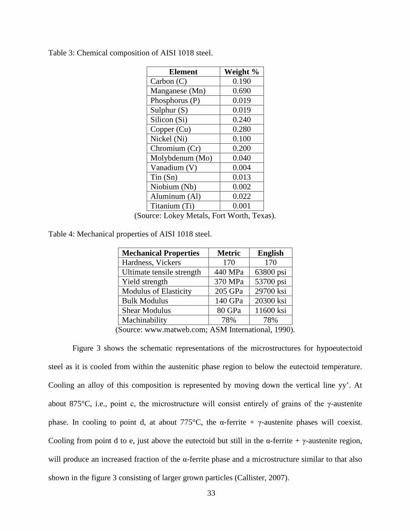
Table 3: Chemical composition of AISI 1018 steel.
Element Weight % Carbon (C) 0.190 Manganese (Mn) 0.690 Phosphorus (P) 0.019 Sulphur (S) 0.019 Silicon (Si) 0.240 Copper (Cu) 0.280 Nickel (Ni) 0.100 Chromium (Cr) 0.200 Molybdenum (Mo) 0.040 Vanadium (V) 0.004 Tin (Sn) 0.013 Niobium (Nb) 0.002 Aluminum (Al) 0.022 Titanium (Ti) 0.001
(Source: Lokey Metals, Fort Worth, Texas).
Table 4: Mechanical properties of AISI 1018 steel.
Mechanical Properties Metric English Hardness, Vickers 170 170 Ultimate tensile strength 440 MPa 63800 psi Yield strength 370 MPa 53700 psi Modulus of Elasticity 205 GPa 29700 ksi Bulk Modulus 140 GPa 20300 ksi Shear Modulus 80 GPa 11600 ksi Machinability 78% 78%
(Source: www.matweb.com; ASM International, 1990).
Figure 3 shows the schematic representations of the microstructures for hypoeutectoid
steel as it is cooled from within the austenitic phase region to below the eutectoid temperature.
Cooling an alloy of this composition is represented by moving down the vertical line yy’. At
about 875°C, i.e., point c, the microstructure will consist entirely of grains of the γ-austenite
phase. In cooling to point d, at about 775°C, the α-ferrite + γ-austenite phases will coexist.
Cooling from point d to e, just above the eutectoid but still in the α-ferrite + γ-austenite region,
will produce an increased fraction of the α-ferrite phase and a microstructure similar to that also
shown in the figure 3 consisting of larger grown particles (Callister, 2007).
33

Figure 3: Schematic representation of microstructures for AISI 1018 steel.
As the temperature is lowered just below the eutectoid, to point f, all the γ-austenite
phase will transform to pearlite. There will be no change in the α-ferrite phase; it will be present
in the form of continuous matrix phase surrounding the isolated pearlite colonies. The ferrite
phase will be present both in the pearlite and also as the phase that formed while cooling through
α-ferrite + γ-austenite phase region. The ferrite that is present in the pearlite is called eutectoid
ferrite, whereas the other, that was formed before eutectoid is termed as proeutectoid ferrite
(Callister, 2007). The pearlite has a lamellar structure which consists of α-ferrite and Fe3C.
Figure 4 shows a SEM image of as-received AISI 1018 steel, with clearly marked
proeutectoid ferrite and pearlite. A magnified image of the iron carbide showing the lamellar
structure is also shown in figure 4. Figure 5 gives us a much clear picture of the pearlite with a
34

clear distinction of the α-ferrite and Fe3C (Iron carbide/Cementite).
Figure 4: SEM image of as-received AISI 1018 steel.
Figure 5: TEM image of pearlite.
35

End Milling Equipment
A CNC Mori Seiki Dura Vertical 5060 machining center was used to perform the end
milling operation for this study. Figure 6 shows the machine in idle condition.
The following are the specifications of the machining center:
• Manufacturer: Mori Seiki
• Machine type: Vertical milling machine
• NC controller: Fanuc MSX-504 III
• Maximum power: 15 HP
• Maximum spindle speed: 10000 RPM
• Travel range in X x Y x Z-axis: 23.600 x 20.900 x 20.100 inches
Figure 6: Mori Seiki Dura Vertical 5060 machining center.
36

The machining center was equipped with an exhaust pump as shown in figure 6. The
exhaust pump was a Darwin 2000M model, manufactured by Losma, Inc. The machining center
was also equipped with a single nozzle Kuroda Ecosaver KEP3 micro lubrication system as
shown in figure 7. The lubricant flow rate was maintained at 12 ml/h at an air pressure of 0.1
MPa.
Figure 7: Kuroda Ecosaver KEP3 micro lubrication system.
The machining center was equipped with a tool magazine with a maximum storage
capacity of 30 tools. The machining area was fully enclosed when in operation.
Metal Working Fluid (MWF)
Accu-Lube 6000 vegetable-based lubricant was used as a metal working fluid. It is
manufactured by ITW ROCOL North America. The lubricant was specially recommended for
micro lubrication of ferrous and non-ferrous materials. It is manufactured using renewable raw
37

materials and is non-toxic and biodegradable. It is not diluted in water before use. The physical
properties of Accu-Lube 6000 are listed below:
Table 5: Mechanical properties of Accu-Lube 6000.
Mechanical Properties Values Appearance Blue Specific gravity 0.92 Viscosity at 40ºC 8.9 cSt Flash point 418ºF (214ºC) Pour point -40ºF (-40ºC) Pin & Vee block 1250 lbs Sulphur None Chlorine None Silicon None VOC Nil Mineral oil 0% Water solubility Insoluble (Source: ITW Rocol North America, 2012).
Aerosol Mass Concentration and Aerosol Particle Size Measurements
The aerosol mass concentration and aerosol particle size measurements were done using
the Thermo Scientific DataRam4. The DataRam 4 is a portable, high-sensitivity, two-wavelength
nephelometric monitor with a light scattering sensing configuration that has been optimized for
the measurement of the fine particle fraction of airborne dust, smoke, fumes, and mists in
ambient, atmospheric, industrial, research, and indoor environments. The DataRam 4 provides
direct and continuous readout as well as electronic recording of the information gathered
(Thermo Scientific, 2012). The DataRam4 has an aerosol mass concentration measuring range of
0.0001 to 400 mg/m3. The DataRam4 is capable of storing 50,000 data points which include
individual point averages and detecting the median particle size of up to 0.05 μm. Figure 8 shows
the DataRam 4 attached with a non-electrostatic Tygon tube to measure the aerosol mass
concentration and the aerosol particle size produced during the end milling experiments.
38

Figure 8: Thermo scientific DataRam4.
A hole was made on the side of the machine to insert the tygon tube near the machining
area. A rubber grommet was used to seal the hole near the tygon tube. The position of the
DataRam4 and the tygon tube was adjusted properly to minimize the turbulence produced by the
mist during machine operating condition.
Samples Preparation
AISI 1018 steel samples were available in the form of circular blocks of 4 inch diameter
and 1.5 inch thickness. The samples were previously cut from a 10 feet long AISI 1018 steel bar
stock for a drilling study. One side of the circular block already had 1 inch deep drilled holes on
39

it from the earlier experiment. The other side was used for the end milling experiment. The idea
of using the previously drilled workpieces saved a lot of time and money for the study. The final
sample ready for doing end milling experiments is shown in figure 9.
Figure 9: Final sample.
End Milling Procedures
A CNC program was written and inserted into the machining center using the Fanuc NC
controller. Dry runs were conducted to test the program. The Kuroda microlubrication system
was filled with the required coolant (i.e. Accu-Lube 6000) and was set to the flow rate of 12
ml/hr and the air pressure of 0.1 MPa. The nozzle was positioned properly to spray exactly on
the tool-workpiece interface. The tool was inserted in the tool magazine. Before the start of the
end milling process, it was ensured that the workpiece was tightly held in the circular vice and
the machine sliding door was closed. The DataRam4 was also turned ‘ON’. The workpiece to be
drilled were kept randomly on the pallet so that when any sample was selected for the
40

experiments that sample would be a random sample. There should not be any bias in the
experiment.
The end milling procedure is as follows:
1. Select at random a combination of cutting speed and feed rate from table 1.
2. Turn ‘ON’ the machining center (Mori Seiki, Dura vertical 5060).
3. Insert the selected cutting speed and feed rate into the machine through the NC controller.
4. Turn ‘ON’ the exhaust pump.
5. Press the green ‘Cycle Start’ button on the numerical control (NC) controller.
6. Press the ‘Start Run’ button on the DataRam4.
7. After the machining cycle is complete, press the ‘Terminate Run’ button on the
DataRam4.
8. Turn ‘OFF’ the exhaust pump.
9. Open the sliding door.
10. Remove the workpiece from the circular vice.
11. Remove the cutting tool and measure its flank wear by toolmaker’s microscope.
12. If the flank wear is less than the failure criteria load the cutting tool in the tool magazine.
13. Load a new workpiece and repeat Step 4 to 12 until the tool fails.
The tool was declared failed, if the flank wear of any one of the two flanks went above
0.5 mm (ASM International, 1989). If the cutting tool fails, load a new cutting tool in the tool
magazine. Do the tool length compensation for the cutting tool and follow the same end milling
procedure again. Before loading the next component in the circular vice, ensure that the vice is
thoroughly cleaned of chips and coolant. At the end of each day, save all the readings from the
DataRam4 into the computer. All data collected should be saved on a spreadsheet.
41

Method of Data Analysis for MANOVA
MANOVA was conducted to investigate the main and the interaction effects of the
independent variables (namely, cutting speed and feed rate) on all the dependent variables
namely flank wear side 1, flank wear side 2, aerosol mass concentration and aerosol particle size.
Minitab 16 statistical software was used for the data analysis.
The following steps were taken in the MANOVA analysis:
1. Organize and input the data obtained from tool flank wear measurement and the
DataRam4.
2. Verify the MANOVA assumptions by analyzing the ‘Normal plots of residuals’,
‘Residuals versus the fitted values’ and ‘Equality of covariance’.
3. Conduct data transformation if required.
4. Perform the significant test of the independent variables at 95% confidence level.
5. Plot graphs to aid in analyses.
MANOVA Assumptions
1. Data should be randomly sampled from the populations of interest.
2. Observations should be independent of one another.
3. The dependent variables should have a multivariate normal distribution within each
group. The dependent variables should also meet univariate normality assumptions.
4. Equality of covariance matrices of all groups of dependent variables. This assumption is
two-folds:
(i) The ANOVA homogeneity of variance assumption must be met for each
dependent variables;
42
(ii) The correlation between any two dependent variables must be the same in all
groups (Bray & Maxwell, 1985).
Robustness of MANOVA
Although the MANOVA assumptions are mathematical requirements for MANOVA, in
practice it is unlikely that all of the assumptions will be met precisely. Under many conditions in
MANOVA, violating the assumptions does not necessarily invalidate the results. In other words,
MANOVA is relatively robust to violations of the assumptions in many circumstances. However,
MANOVA is not robust to violations of either of the first two assumptions. Departures from
multivariate normality generally have only very slight effects on the Type I error rates of the four
statistics. The sole known exception to this rule is that Roy's greatest characteristic root test may
lead to much Type I errors when only one of several groups has a distribution with high positive
kurtosis. Departures from normality may reduce statistical power. One possible solution to this
problem is to employ transformations of the data to achieve normality (or at least approximate it
more closely), in much the same manner as ANOVA.
The effects of failing to meet the equality of covariance matrices assumption are more
complicated. When sample sizes are unequal, none of the four test statistics is robust. Depending
on the relationship between the sample sizes and the covariance matrices, either too many or too
few Type I errors will result. When sample sizes are equal, all of the test statistics tend to be
robust unless sample sizes are small, or the number of variables is large, and the difference in
matrices is quite large. However, Olson 1974, has found that the Pillai-Bartlett trace is much
more robust across a wide range of population configurations than any of the other three
statistics (Bray & Maxwell, 1985).
43

Hypotheses
1. Null Hypothesis:
There is no significant difference between the responses (i.e. flank wear side 1 & 2,
aerosol mass concentration and aerosol particle size) obtained by varying the individual input
variables (i.e. cutting speed and feed rate).
2. Alternate Hypothesis:
There is a significant difference between the responses (i.e. flank wear side 1 & 2, aerosol
mass concentration and aerosol particle size) obtained by varying the individual input variables
(i.e. cutting speed and feed rate).
Tool Flank Wear Measurements
The cutting tools flank wear measurements were done by Mitutoyo toolmaker’s
microscope. The microscope and a magnified inset image of the tool flank face showing the
flank wear as seen from the microscope is shown in figure 10. The microscope has a maximum
magnification of 40X. The cutting tool was set on the XY-stage with its flank aligned with the Y-
axis as seen from the eyepiece. The microscope has a contour illumination from the bottom
suited for measurement and inspection of specimen contour and a surface illuminator for
observation and inspection of specimen surfaces. A digital micrometer head was attached to the
X and Y-axis and was set to zero. The micrometer was equipped with digital data display which
gave live readings. The Y-Axis was carefully moved in +Y-directions and was aligned with the
maximum flank wear valley as seen on the tool from the eyepiece. Reading from the micrometer
was than collected and recorded in MS-Excel manually.
44

Figure 10: Mitutoyo toolmaker’s microscope.
The toolmaker’s microscope was also equipped with a camera to take pictures of the
specimen. The camera can be fixed on the eyepiece. A picture taken from the camera is shown in
figure 11 with the cutting tool rake face of side 2 for treatment 100 SFM and 0.003 IPT.
45

Figure 11: Optical micrograph of tool rake side 1 - Treatment 100 SFM and 0.003 IPT.
Tool-Workpiece Interface Temperature Calculations
The interface temperature between the cutting tool and the workpiece was calculated
using peclet numbers. When the cutting tool and the workpiece are in contact the interface
experiences a rise in temperature. The mechanical energy which is required to overcome the
frictional resistance during machining is dissipated through a conversion into thermal energy and
is responsible for the tool-workpiece interface temperature rise. This increase in temperature can
sometime even lead to cutting tool failure. The temperature rise is of very short durations and is
called ‘flash temperature’. The presence of the lubricant in the tool-workpiece interface will
affect the temperature rise. Some part of the heat will be convected away by the lubricant,
resulting in the cooling of the interface. Therefore, an accurate value of the coefficient of friction
is very difficult to obtain; however, in most lubricated contacts the coefficient of friction is <0.1
(Stachowiak & Batchelor, 2005).
There is no single algebraic equation giving the flash temperature for the whole range of
surface velocities and contact geometries. A non-dimensional measure of the speed at which the
46

two surface moves across each other called the ‘Peclet number’ is used as a criterion allowing
the differentiation between various speed regimes and contact geometries.
The peclet number (Stachowiak & Batchelor, 2005) is defined as:
Pe (Peclet #) = Ua/2χ
where:
Pe = peclet number;
U = velocity of solid (workpiece or tool) [m/s];
a = contact dimension [m], (i.e. contact radius for circular contacts, half width of the
contact square for square contacts and the half width of the rectangle for linear
contacts); here a = (4 W R'L π E'
)2 where:
W = normal load, here = mg;
R’ = reduced area of curvature, here = (1/Rtool) + (1/Rworkpiece)
E’ = reduced young’s modulus, here = {(1-νtool2)/Etool} + {(1-νworkpiece
2)/Eworkpiece}
E = young’s modulus
χ = thermal diffusivity [m2/s]. i.e., χ = κ/ρσ, where:
κ = thermal conductivity [W/mK];
ρ = density [kg/m3];
σ = specific heat [J/kgK].
Peclet number is the ratio of speed of the surface to the rate of thermal diffusion into the
solid. It is an indicator of the heat penetration into the bulk of the contacting solid, i.e., it
describes whether there is sufficient time for the surface temperature distribution of the contact
to diffuse into the stationary solid. A higher Peclet number indicates a higher surface velocity for
constant materials characteristics.
47

The heat transfer effects vary with the Peclet number. The following velocity ranges,
defined by their Peclet number, are considered in flash temperature analysis (Stachowiak &
Batchelor, 2005):
Pe < 0.1 one surface moves very slowly with respect to the other. There is enough time for
the temperature distribution of the contact to be established in the stationary body,
i.e., steady state conduction.
0.1 < Pe < 5 intermediate region one surface moves fast with respect to other, and a slowly
moving heat source model is assumed.
Pe > 5 one surface moves fast with respect to other and is modeled by a fast moving heat
source. There is insufficient time for temperature distribution of the contact to be
established in the stationary body. The depth to which the heat penetrates into the
stationary body is very small compared to the contact dimensions.
The heat partition or proportion of heat (Ƞ) in the workpiece and the tool can be calculated by,
Ƞworkpiece = 1/ 1+( κtool x √Petool / κworkpiece x √Peworkpiece)
Note that the Pe can be dropped from the equation if the value of Pe is very low.
Table 6: Average and maximum flash temperature formulae for line contacts (Stachowiak & Batchelor, 2005).
Peclet number Average flash temperature Tfa Maximum flash temperature Tfmax
L < 0.1 0.318 × µ W (Ua−Ub)Kl
× χUb
× (-2.303 L Log10 2 Pe + 1.616 Pe)
0.318 × µ W (Ua−Ub)Kl
× χUb
× (-2.303 L Log10 Pe + 1.616Pe)
0.1 < L < 5 0.159 C3 × µ W (Ua−Ub)Kl
× χUb
(where C3 = 1.1)
0.159 C4 × µ W (Ua−Ub)Kl
× χUb
(where C4 = 1.3)
L > 5 0.266 × µ W (Ua−Ub)Kl
× ( χUb
)0.5 0.399 × µ W (Ua−Ub)Kl
× ( χUb
)0.5
48

Flash temperature formulae for line contacts for various velocity ranges are summarized
in table 6.
where:
µ = coefficient of friction;
Ua, Ub = surface velocities of solid ‘A’ (i.e. workpiece) and solid ‘B’ (i.e. tool);
l = half length of the line contact [m]
Flash temperature equations are given in terms of the heat supply over the contact area,
the velocity and the thermal properties of the materials. They are derived based on the
assumption that the proportion of the total heat flowing into each contacting body is that the
average temperature over the contact area is the same for both bodies.
The next step is to calculate the true flash temperature rise and maximum flash
temperature rise. The true flash temperature rise must be the same for both the solids in contact
and is calculated from:
1/Tf = 1/Tfworkpiece + 1/Tftool
The maximum temperature rise is calculated by the formulae:
1/Tfmax = 1/(Tfmax)workpiece + 1/(Tfmax)tool
Vickers Hardness Measurement
The hardness measurements were carried out using Shimadzu dynamic ultra micro
hardness tester model # DUH-211S as shown in figure 12. The hardness tester is equipped with
an optical microscope and a X and Y-axis micrometer. The hardness tester uses a standard type
115º standard pyramid indenter. Electromagnetic force is used to press the indenter against a
specimen. The pressing force is increased at a constant rate, from 0 to the preset test force. The
49
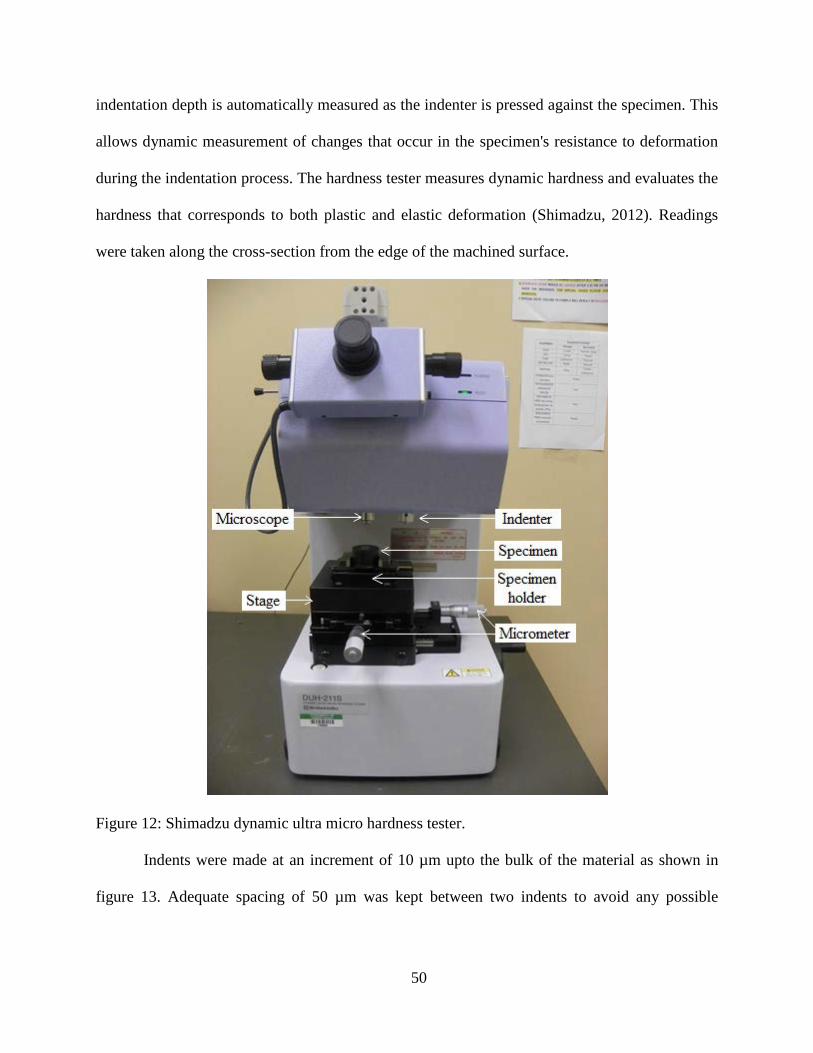
indentation depth is automatically measured as the indenter is pressed against the specimen. This
allows dynamic measurement of changes that occur in the specimen's resistance to deformation
during the indentation process. The hardness tester measures dynamic hardness and evaluates the
hardness that corresponds to both plastic and elastic deformation (Shimadzu, 2012). Readings
were taken along the cross-section from the edge of the machined surface.
Figure 12: Shimadzu dynamic ultra micro hardness tester.
Indents were made at an increment of 10 µm upto the bulk of the material as shown in
figure 13. Adequate spacing of 50 µm was kept between two indents to avoid any possible
50

alteration in readings due to the deformation caused by the earlier indent. Gradient in the
hardness values was reported.
Figure 13: Schematic of vickers hardness measurements.
Bakelite mounts as shown in figure 14, were made to make sure that the material does not
bulge out while taking the readings near to the edge of the cross-sectional machined surface.
Figure 14: Bakelite mount.
50µm
10µm
Cutting tool
Machined surface
Workpiece
Tool rotation
Indents
Cross-section
10µm
50µm
Machined surface
Cross-section
51

Bearing Area Curve Measurement
A Nanovea non-contact optical profilometer was used to get the bearing area curve
(BAC). The optical profilometer is shown in figure 15. BAC is a statistical method to represent
the machined surface topography. It was introduced by Abbott and Firestone in 1933. Hence, it is
also called as ‘Abbott Curve’. The BAC can approximate the real contact area obtained from the
surface profile. It is compiled by considering the fraction of surface profile intersected by an
infinitesimally thin plane positioned above a datum plane. The intersect length with material
along the plane is measured, summed together and plotted as a proportion of the total length. The
obtained curve is an integral of the height probability density function and if the height
distribution is Gaussian, then this curve is nothing else than the cumulative probability
distribution function (CDF) (Stachowiak & Batchelor, 2005).
Figure 15: Nanovea non-contact optical profilometer.
52
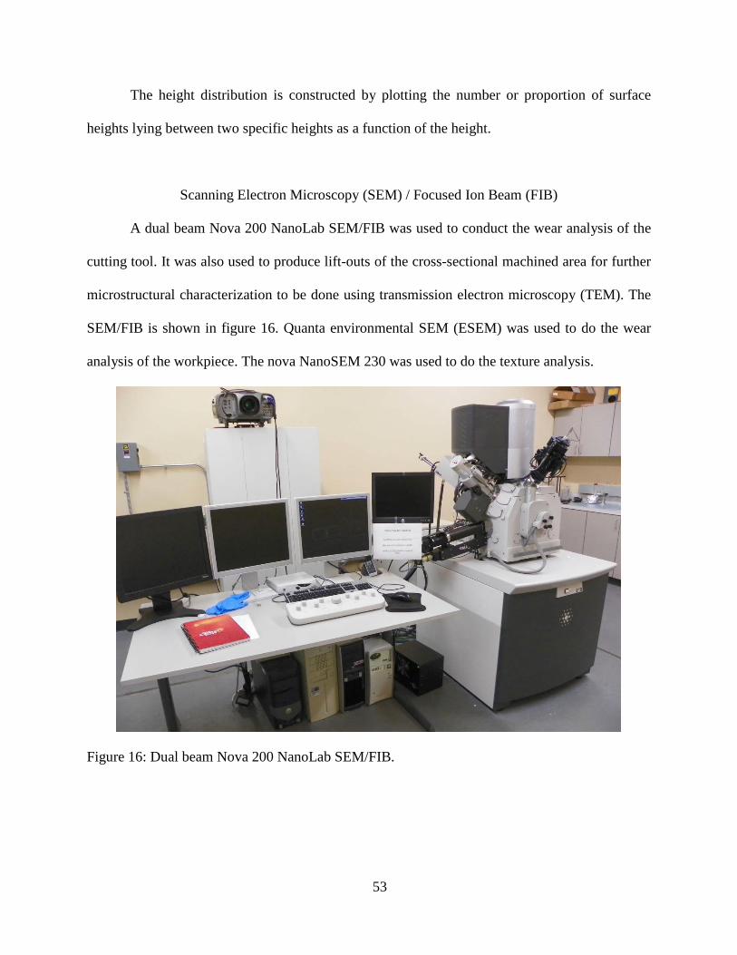
The height distribution is constructed by plotting the number or proportion of surface
heights lying between two specific heights as a function of the height.
Scanning Electron Microscopy (SEM) / Focused Ion Beam (FIB)
A dual beam Nova 200 NanoLab SEM/FIB was used to conduct the wear analysis of the
cutting tool. It was also used to produce lift-outs of the cross-sectional machined area for further
microstructural characterization to be done using transmission electron microscopy (TEM). The
SEM/FIB is shown in figure 16. Quanta environmental SEM (ESEM) was used to do the wear
analysis of the workpiece. The nova NanoSEM 230 was used to do the texture analysis.
Figure 16: Dual beam Nova 200 NanoLab SEM/FIB.
53

Electron Backscatter Diffraction (EBSD)
EBSD technique was carried out in the NanoSEM 230. EBSD is a SEM based
microstructural crystallographic technique. In EBSD, an electron beam strikes a predetermined
location on a tilted sample and the diffracted electrons form a pattern on a fluorescent screen.
This pattern is characteristic of the crystal structure and orientation of the sample region from
which it is generated. It provides the crystal orientation with sub-micron resolution down to ~ 50
nm (Oxford Instruments, 2013). The EBSD analysis was done to measure the grain size, phase
mapping and potential grain texture. Electropolishing was done before mounting the samples for
EBSD analysis. A solution containing 90% acetic acid and 10% perchloric acid was used for
etching the surface for 300 seconds. Samples were than cleaned in an ultrasonicator and mounted
on an SEM sample stub for EBSD analysis.
Transmission Electron Microscopy (TEM)
A Tecnai G2 F20 TEM was used to do the subsurface deformation structural evolution
analyses of the machined cross-sectional area. The TEM is shown in figure 17 (a). Electron
transparent samples were made in SEM/FIB after attaching them on a Cu grid. The Cu grid are
inserted into the TEM sample holder. High energy electrons are transmitted having very small
wavelength (i.e., 0.025Aº) through the sample to image the microstructure of the material with
high resolution. Line defects, interfaces, grain boundaries, morphologies, crystallographic phases
and defects can be observed using TEM.
54

Figure 17 (a): Tecnai G2 F20 TEM.
Dislocation Density Quantification Procedure
The dislocation density was calculated by the line intersection method (Roy et al. 2006)
which was based on the superimposition of the grid consisting of the horizontal and vertical lines
on a TEM micrograph containing dislocations. The magnitude of the total length of the
horizontal (∑ Lh) and vertical (∑ Lv) test lines were determined from the test grid, while the
thickness (t) of the TEM specimen was determined by the convergent beam electron diffraction
(CBED) method (Williams & Carter, 2009). When exactly on a two-beam condition, the
transmitted undiffacted beam (000) - disc usually contains concentric diffuse fringes known as
Kossel-Mollenstedt (K-M) fringes. The number of fringes increases by one every time the
55

thickness increases by one extinction distance. The thickness measurements are not made under
the zone axis but under two beam conditions with only one strongly excited (hkl) reflection. The
CBED will contain parallel instead of concentric intensity oscillations (Liao, 2006) as shown in
figure 17 (b).
Figure 17 (b): Necessary measurements to extract thickness (t) from K-M fringes.
The central bright fringe is in exact Bragg condition. The fringe spacing corresponds to
angle ΔΘi and from this spacing the deviation si for ith fringe can be determined using Eq. 1.
si = 𝜆 ΔΘi2𝛩𝑏𝑑2
(1)
where,
λ = wavelength of the incident electron
56

Θb = the Bragg angle for the diffracting (hkl) plane
d = the (hkl) interplanar spacing
If the extinction distance ξg is known, the foil thickness (t) can be determined according
to Eq. 2,
𝑆𝑖2
nk2+ 1
ξg2nk2= 1
t2 (2)
where,
nk = integer
If the extinction distance is not known, then a graphical method is used to plot the
measurements for several fringes as follows (Williams & Carter, 2009):
• Arbitrarily assign the integer n = 1 to the first fringe to an excitation error si.
• Then assign n = 2 to the second fringe, s2, etc.
• Plot (si/nk)2 versus (1/nk)2. If the result is a straight line, the arbitrary assignment was
good.
• If the plot is a curve, then repeat the procedure by re-assigning n = 2 to the first fringe.
• Continue to iterate until you find a straight line as shown in figure 17 (b)
After calculating the foil thickness, the dislocation density (ρ) was calculated by using
Eq. 3.
ρ = 1t (∑nv∑Lv
+ ∑nh∑Lh
) (3)
where,
∑ nv = number of intersections of vertical test lines with the dislocations
∑ nh = number of intersections of horizontal test lines with the dislocations
∑ Lv = total length of vertical test lines
57

∑ Lh = total length of horizontal test lines
Assumptions of the Study
1. Any lack of rigidity in the machine tool and set up did not affect the data in the study.
2. Position of the mister nozzle and the flow rate was consistently same throughout the
study.
3. Use of the toolmaker’s microscope, DataRam4 and the vickers hardness tester was
consistent throughout the study.
4. Tool flank wear was an appropriate indicator of tool life.
5. MANOVA was the appropriate statistical technique used for the analysis.
6. All the cutting tools and coatings used in the study were identical in composition.
7. The as-received workpiece material composition was homogeneous.
58
CHAPTER 4
RESULTS AND ANALYSES
This chapter includes the results of multivariate analysis of variance (MANOVA), tool-
workpiece interface temperature analysis, tool life, wear mechanisms, cross-sectional hardness
analysis at failure, transmission electron microscopy (TEM) analysis at failure, dislocation
density quantification and electron backscattered diffraction (EBSD) analysis.
MANOVA
Minitab 16 statistical software was used for the MANOVA analysis. The flank wear side
1, side 2, aerosol mass concentration and aerosol particle size data was first checked for the
MANOVA assumptions. The homogeneity of covariance was determined using Bartlett’s test
and Levene’s test at 95% confidence level. The results are shown in Figures 18, 19, 20 and 21
for flank wear side 1, side 2, aerosol mass concentration and aerosol particle size, respectively.
The p-values of Bartlett and Levene’s test for all the dependent variables are significant
indicating that they meet the equality of covariance assumption. Figures 22, 23, 24 and 25, show
plots of residual versus fitted values which were used to test the assumption of constant variance
for flank wear side 1, side 2, aerosol mass concentration and aerosol particle size. To fulfill the
test, these plots should be a random scatter. The constant variance in the data demonstrates that
the data does not follow a particular pattern, indicating constant variance.
59

Figure 18: Test for equal covariance for flank wear side 1.
Figure 19: Test for equal covariance for flank wear side 2.
Speed Feed
120.0
100.0
80.0
0.005
0.003
0.005
0.003
0.005
0.003
0.50.40.30.20.10.0
95% Bonferroni Confidence Intervals for StDevs
Test Statistic 9.19P-Value 0.057
Test Statistic 0.94P-Value 0.465
Bartlett's Test
Levene's Test
Speed Feed
120.0
100.0
80.0
0.005
0.003
0.005
0.003
0.005
0.003
108642095% Bonferroni Confidence Intervals for StDevs
Test Statistic 3.99P-Value 0.408
Test Statistic 0.59P-Value 0.676
Bartlett's Test
Levene's Test
60

Figure 20: Test for equal covariance for aerosol mass concentration.
Figure 21: Test for equal covariance for aerosol particle size.
Speed Feed
120.0
100.0
80.0
0.005
0.003
0.005
0.003
0.005
0.003
161412108642095% Bonferroni Confidence Intervals for StDevs
Test Statistic 8.39P-Value 0.078
Test Statistic 0.98P-Value 0.441
Bartlett's Test
Levene's Test
Speed Feed
120.0
100.0
80.0
0.005
0.003
0.005
0.003
0.005
0.003
2.52.01.51.00.50.095% Bonferroni Confidence Intervals for StDevs
Test Statistic 6.27P-Value 0.180
Test Statistic 1.65P-Value 0.206
Bartlett's Test
Levene's Test
61
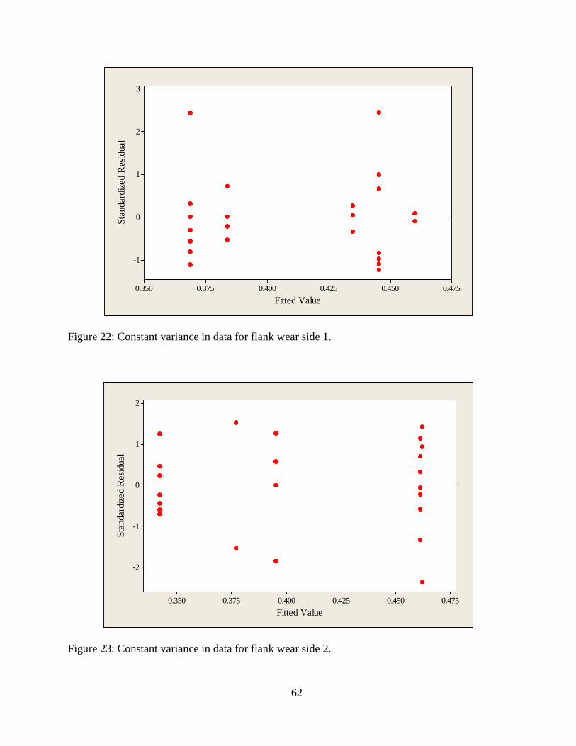
Figure 22: Constant variance in data for flank wear side 1.
Figure 23: Constant variance in data for flank wear side 2.
0.4750.4500.4250.4000.3750.350
3
2
1
0
-1
Fitted Value
Stan
dard
ized
Res
idua
l
0.4750.4500.4250.4000.3750.350
2
1
0
-1
-2
Fitted Value
Stan
dard
ized
Res
idua
l
62

Figure 24: Constant variance in data for aerosol mass concentration.
Figure 25: Constant variance in data for aerosol particle size.
7.67.47.27.06.86.66.46.26.0
2
1
0
-1
-2
Fitted Value
Stan
dard
ized
Res
idua
l
0.780.770.760.750.74
2
1
0
-1
-2
Fitted Value
Stan
dard
ized
Res
idua
l
63

Mahalanobis distance was used to test the data for multivariate normality. An observation
is classified into a group if its Mahalanobis distance is the minimum. The outlier plot, as shown
in figure 26 displays Mahalanobis distances for each observation. Points that fall above the y-
axis reference line are outliers. There do not appear to be any outliers in the data.
Figure 26: Mahalanobis distance for multivariate normality testing for flank wear side 1, side 2, aerosol mass concentration and aerosol particle size.
Data was also examined for univariate normality assumption for analysis of variances
(ANOVA). A normal probability plot was used to determine if the distribution of data
approximates a normal distribution. In the ANOVA, the normal probability plot is usually more
effective and straightforward when it is done with residuals. The normal probability plot of
residuals for flank wear side 1, side 2, aerosol mass concentration and aerosol particle size is
shown in figures 27, 28, 29 and 30. The residual is the difference between the actual and
predicted response values. The normal probability plot with a general straight line pattern
indicates that the residuals follow a normal distribution. The far points which are slightly
2520151050
3.5
3.0
2.5
2.0
1.5
1.0
0.5
0.0
Observation
Mah
alan
obis
Dis t
ance
3.403
64

scattered do not follow any significant pattern. The ANOVA is said to be robust for the
normality assumption.
Figure 27: Normal plots of residual in data for flank wear side 1.
3210-1-2
99
9590
80706050403020
105
1
Standardized Residual
Perc
ent
Normal Probability Plot
65

Figure 28: Normal plots of residual in data for flank wear side 2.
Figure 29: Normal plots of residual in data for aerosol mass concentration.
3210-1-2-3
99
9590
80706050403020
105
1
Standardized Residual
Perc
ent
Normal Probability Plot
3210-1-2-3
99
9590
80706050403020
105
1
Standardized Residual
Perc
ent
Normal Probability Plot
66

Figure 30: Normal plots of residual in data for aerosol particle size.
The MANOVA results are shown in table 7. The MANOVA model selected gave the
main factors effects and the 2-way interaction effects.
Table 7: MANOVA test summarized results.
General Linear Model (MANOVA)
Source Criterion Test Statistics
F Value
Numerator DF
Denominator DF
p- value Result
Speed Pillai’s 0.90714 3.320 8 30 0.007 Significant Feed Pillai’s 0.89738 32.793 4 15 0.000 Significant
Speed*Feed Pillai’s 0.55631 1.541 8 32 0.182 Not Significant
The model gave an F-value of 3.32, 32.79 and 1.54 for speed, feed and the interaction of
(speed*feed), respectively. A significant effect is one that has a probability of occurrence (i.e. p-
value) less than or equal to 0.05. Table 7 indicates that the speed and feed variables main effects
are significant at 95% confidence level. But, the interaction of (speed*feed) was not significant
at 95% confidence level. Univariate ANOVA was performed to determine which of the
dependent variables were significantly affected by the independent variable. Tables 8, 9, 10 and
210-1-2
99
9590
80706050403020
105
1
Standardized Residual
Perc
ent
Normal Probability Plot
67
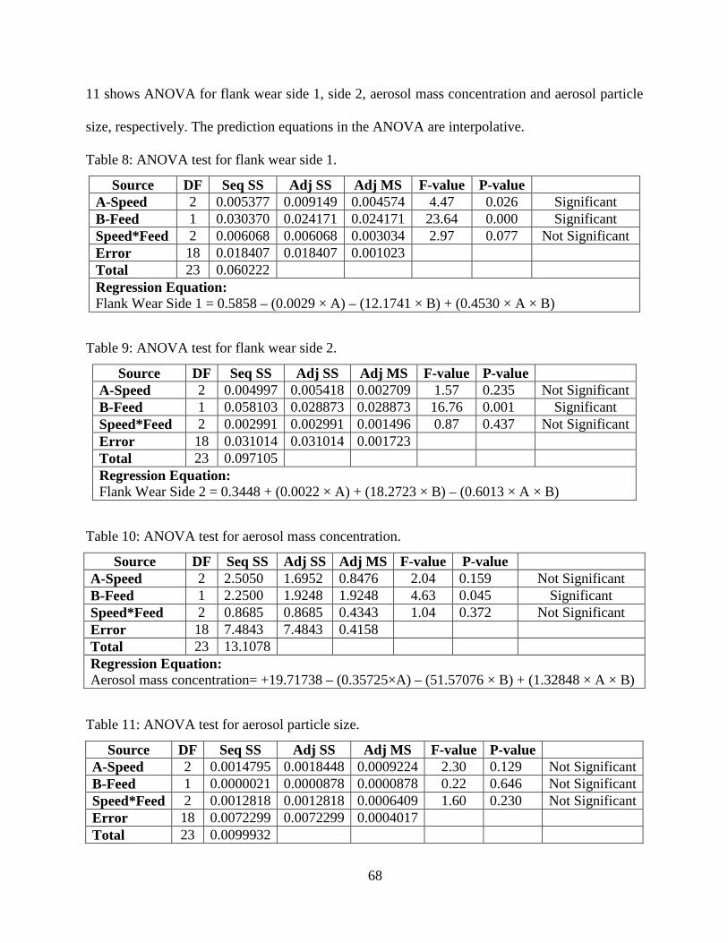
11 shows ANOVA for flank wear side 1, side 2, aerosol mass concentration and aerosol particle
size, respectively. The prediction equations in the ANOVA are interpolative.
Table 8: ANOVA test for flank wear side 1.
Source DF Seq SS Adj SS Adj MS F-value P-value A-Speed 2 0.005377 0.009149 0.004574 4.47 0.026 Significant B-Feed 1 0.030370 0.024171 0.024171 23.64 0.000 Significant Speed*Feed 2 0.006068 0.006068 0.003034 2.97 0.077 Not Significant Error 18 0.018407 0.018407 0.001023 Total 23 0.060222 Regression Equation: Flank Wear Side 1 = 0.5858 – (0.0029 × A) – (12.1741 × B) + (0.4530 × A × B)
Table 9: ANOVA test for flank wear side 2.
Source DF Seq SS Adj SS Adj MS F-value P-value A-Speed 2 0.004997 0.005418 0.002709 1.57 0.235 Not Significant B-Feed 1 0.058103 0.028873 0.028873 16.76 0.001 Significant Speed*Feed 2 0.002991 0.002991 0.001496 0.87 0.437 Not Significant Error 18 0.031014 0.031014 0.001723 Total 23 0.097105 Regression Equation: Flank Wear Side 2 = 0.3448 + (0.0022 × A) + (18.2723 × B) – (0.6013 × A × B)
Table 10: ANOVA test for aerosol mass concentration.
Source DF Seq SS Adj SS Adj MS F-value P-value A-Speed 2 2.5050 1.6952 0.8476 2.04 0.159 Not Significant B-Feed 1 2.2500 1.9248 1.9248 4.63 0.045 Significant Speed*Feed 2 0.8685 0.8685 0.4343 1.04 0.372 Not Significant Error 18 7.4843 7.4843 0.4158 Total 23 13.1078 Regression Equation: Aerosol mass concentration= +19.71738 – (0.35725×A) – (51.57076 × B) + (1.32848 × A × B)
Table 11: ANOVA test for aerosol particle size.
Source DF Seq SS Adj SS Adj MS F-value P-value A-Speed 2 0.0014795 0.0018448 0.0009224 2.30 0.129 Not Significant B-Feed 1 0.0000021 0.0000878 0.0000878 0.22 0.646 Not Significant Speed*Feed 2 0.0012818 0.0012818 0.0006409 1.60 0.230 Not Significant Error 18 0.0072299 0.0072299 0.0004017 Total 23 0.0099932
68

The ANOVA for flank wear side 1 shown in table 8 indicates that the speed and feed
variables main effects are statistically significant at 95% confidence level while the interaction of
(speed*feed) is not statistically significant at 95% confidence level. The resulting model gave an
R-squared value of 0.6944 indicating that it is able to predict 69.44% of the variation in the data.
The remaining percent is considered noise and may not be predicted by this model. The sources
of which may be manual variations while taking flank wear readings, machine vibrations,
variations within the tools and workpiece materials.
The ANOVA for flank wear side 2 shown in table 9 indicates that the feed variable main
effects is statistically significant at 95% confidence level while the speed variables main effect
and the interaction of (speed*feed) are not statistically significant at 95% confidence level. The
resulting model gave an R-squared value of 0.6806 indicating that it is able to predict 68.06% of
the variation in the data. The remaining percent is considered noise and may not be predicted by
this model. The sources of which may be the same as given for flank wear side 1. The units of
the prediction equations for both the flank wear side 1 and 2 are in millimeters (mm).
It was observed that the cutting speed variable main effect for flank wear side 1 was
statistically significant, while the cutting speed variable main effect for flank wear side 2 was
statistically not significant. The reason behind these results is hypothesized to be the alternate
use of up-milling and down-milling cut. As shown in the figure 31, it is always more favorable to
apply down-milling rather than up-milling. When the cutting edge goes into contact in down-
milling, the chip thickness has its maximum value, in up-milling the chip thickness is zero. The
tool life is generally shorter in up-milling due to the fact that there is considerably more heat
generated due to the rubbing action that takes place on the entry. The radial forces are also
considerably higher in up-milling (Sandvik Coromant, 2007).
69

Figure 31: Down-milling (Climb milling) and Up-milling (Conventional milling).
The ANOVA for aerosol mass concentration shown in table 10 indicates that the feed
variables main effects is statistically significant at 95% confidence level while the speed and the
interaction of (speed*feed) is not statistically significant at 95% confidence level. The resulting
model gave an R-squared value of 0.4290 indicating that it is able to predict 42.90% of the
variation in the data. The remaining percent is considered noise and may not be predicted by this
model. The sources of which may be length of the tygon tube, turbulence in aerosol flow due to
unavoidable bends in the tygon tube, type of lubricant, lubricant delivery method, aerosol flow
rate and/or nozzle position. Some of the other reasons may include logging time difference due
to manually turning ON/OFF the exhaust pump and/or DataRam4 particulate monitor, and the
slight difference in positioning of the tygon tube before starting each experiment. The ANOVA
for aerosol particle size shown in table 11 indicates that the speed, feed variable main effects and
the interaction of (speed*feed) are not statistically significant at 95% confidence level. The unit
of the prediction equation for the aerosol mass concentration is in mg/m3.
70
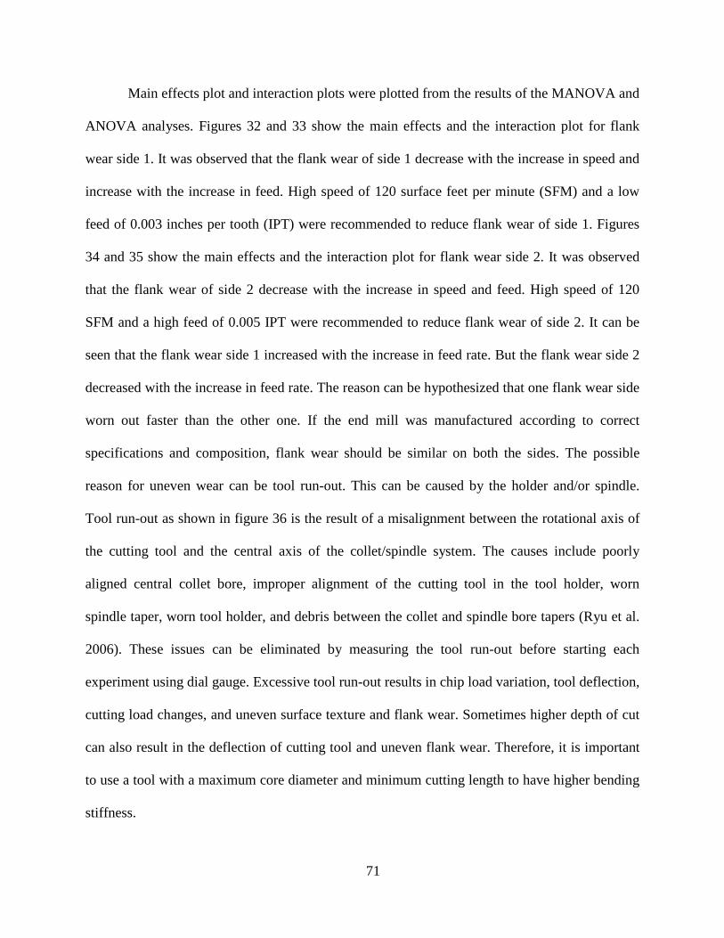
Main effects plot and interaction plots were plotted from the results of the MANOVA and
ANOVA analyses. Figures 32 and 33 show the main effects and the interaction plot for flank
wear side 1. It was observed that the flank wear of side 1 decrease with the increase in speed and
increase with the increase in feed. High speed of 120 surface feet per minute (SFM) and a low
feed of 0.003 inches per tooth (IPT) were recommended to reduce flank wear of side 1. Figures
34 and 35 show the main effects and the interaction plot for flank wear side 2. It was observed
that the flank wear of side 2 decrease with the increase in speed and feed. High speed of 120
SFM and a high feed of 0.005 IPT were recommended to reduce flank wear of side 2. It can be
seen that the flank wear side 1 increased with the increase in feed rate. But the flank wear side 2
decreased with the increase in feed rate. The reason can be hypothesized that one flank wear side
worn out faster than the other one. If the end mill was manufactured according to correct
specifications and composition, flank wear should be similar on both the sides. The possible
reason for uneven wear can be tool run-out. This can be caused by the holder and/or spindle.
Tool run-out as shown in figure 36 is the result of a misalignment between the rotational axis of
the cutting tool and the central axis of the collet/spindle system. The causes include poorly
aligned central collet bore, improper alignment of the cutting tool in the tool holder, worn
spindle taper, worn tool holder, and debris between the collet and spindle bore tapers (Ryu et al.
2006). These issues can be eliminated by measuring the tool run-out before starting each
experiment using dial gauge. Excessive tool run-out results in chip load variation, tool deflection,
cutting load changes, and uneven surface texture and flank wear. Sometimes higher depth of cut
can also result in the deflection of cutting tool and uneven flank wear. Therefore, it is important
to use a tool with a maximum core diameter and minimum cutting length to have higher bending
stiffness.
71

Figure 32: Main effect plot for flank wear side 1.
Figure 33: Interaction plot for flank wear side 1.
120.0100.080.0
0.46
0.45
0.44
0.43
0.42
0.41
0.40
0.39
0.380.0050.003
Speed
Mea
n
Feed
Main Effects Plot for Flank Wear Side 1
0.0050.003
0.50
0.45
0.40
0.35
120.0100.080.0
0.50
0.45
0.40
0.35
Speed
Feed
80.0100.0120.0
Speed
0.0030.005
Feed
Interaction Plot for Flank Wear Side 1
72

Figure 34: Main effect plot for flank wear side 2.
Figure 35: Interaction plot for flank wear side 2.
120.0100.080.0
0.44
0.43
0.42
0.41
0.40
0.39
0.38
0.37
0.36
0.35
0.0050.003
Speed
Mea
n
Feed
Main Effects Plot for Flank Wear Side 2
0.0050.003
0.450
0.425
0.400
0.375
0.350
120.0100.080.0
0.450
0.425
0.400
0.375
0.350
Speed
Feed
80.0100.0120.0
Speed
0.0030.005
Feed
Interaction Plot for Flank Wear Side 2
73

Figure 36: Tool run-out.
Figure 37: Main effect plot for aerosol mass concentration.
120.0100.080.0
7.0
6.8
6.6
6.4
6.2
6.00.0050.003
Speed
Mea
n
Feed
Main Effects Plot for Concentration
74

Figure 38: Interaction plot for aerosol mass concentration.
Figures 37 and 38 show the main effects and the interaction plot for aerosol mass
concentration. It was observed that the aerosol mass concentration decreases with the increase in
speed and feed. High speed of 120 SFM and a high feed of 0.005 IPT were recommended to
reduce the aerosol mass concentration.
The parameter optimization was done by setting the goal to minimize flank wear side 1,
side 2 and aerosol mass concentration. Design Expert 8 software was used to do the parameter
optimization. Figures 39 and 40, show that there is 84.2% desirability to achieve a flank wear
side 1 of 0.365 mm using a cutting speed of 120 SFM and a feed rate of 0.003 IPT. Figures 41
and 42, show that there is 60.7% desirability to achieve a flank wear side 2 of 0.380 mm using a
cutting speed of 120 SFM and 0.0041 IPT. All the figures with optimization parameter show
International System of Units (SI units).
0.0050.0037.6
7.2
6.8
6.4
6.0
120.0100.080.0
7.6
7.2
6.8
6.4
6.0
Speed
Feed
80.0100.0120.0
Speed
0.0030.005
Feed
Interaction Plot for Concentration
75

Figure 39: Desirability plot for flank wear side 1.
Figure 40: Selected solution plot for flank wear side 1.
76

Figure 41: Desirability plot for flank wear side 2.
Figure 42: Selected solution plot for flank wear side 2.
77

Figures 43 and 44 show that there is 84.0% desirability to achieve a concentration of 5.91
mg/m3 using a cutting speed of 120 SFM and a feed rate of 0.005 IPT.
Figure 43: Desirability plot for aerosol mass concentration.
Figure 44: Selected solution plot for aerosol mass concentration.
78

Aerosol Mass Concentration and Aerosol Particle Size Analysis
Figures 45 and 46 show the average mass concentration and the average particle size,
respectively, for different cutting speed and feed rate combinations. Machining with lower speed
and feed rate combinations (i.e. 80 SFM and 0.003 IPT) resulted in the higher average mass
concentration and machining with higher speed and feed rate combinations (i.e. 120 SFM and
0.005 mm/rev) resulted in the lower average mass concentration. The highest average mass
concentration of 8.32 mg/m3 was realized using treatment 80 SFM and 0.003 IPT. At low speed
and feed rates it is hypothesized that atomization is dominant and plays a larger role in aerosol
generation during the cutting process. The particles are less scattered resulting in higher mass
concentration (Jayal et al. 2004). At low speeds and feeds, the resulting mist particles have less
tendency to split, hence resulting in larger size particles as shown in figure 46. The lowest
average mass concentration of 5.91 mg/m3 was realized using treatment 120 SFM and 0.005 IPT.
At high speed and feed rate it is hypothesized that vaporization/condensation are the dominant
mechanisms for the generation of mist. At high speed and feed rate levels the resulting heat is
partially transferred to the lubricant which vaporizes some of the mist particles. Hence a lower
average mass concentration (Sutherland et al. 2000).
Figure 45: Average mass concentration for different cutting speeds and feed rates combinations.
8.32
6.45 6.47 6.20 6.16
5.91
5.00
5.50
6.00
6.50
7.00
7.50
8.00
8.50
9.00
80 SFM 0.003 IPT
100 SFM 0.003 IPT
120 SFM 0.003 IPT
80 SFM 0.005 IPT
100 SFM 0.005 IPT
120 SFM 0.005 IPT
Average Mass
Concentration (mg/m3)
79

Figure 46: Average particle size for different cutting speeds and feed rates combinations
Tool-Workpiece Interface Temperature Analysis
The interface temperature between the cutting tool and the workpiece was calculated
using Peclet numbers as described in chapter 3.
First, low cutting speed (i.e. 80 SFM) and low feed rate (i.e. 0.003 IPT) combination is
considered. We will start our calculation by finding the values of R’, E’, a, χworkpiece and χtool.
So,
R’ = 1 / {(1/Rtool) + (1/Rworkpiece)}
here, Rtool = 0.0254 m and
Rworkpiece = 0.1016 m
∴ R’ = 1 / {(1/0.0254) + (1/0.1016)}
∴ R’ = 0.02032 m
Also,
E’ = 1 / {(1-νtool2)/Etool} + {(1-νworkpiece
2)/Eworkpiece}
here, νtool = 0.26 Etool = 620 GPa
0.758 0.739 0.750
0.777
0.735 0.740
0.60
0.65
0.70
0.75
0.80
80 SFM 0.003 IPT
100 SFM 0.003 IPT
120 SFM 0.003 IPT
80 SFM 0.005 IPT
100 SFM 0.005 IPT
120 SFM 0.005 IPT
Average Particle
Size (microns)
80

νworkpiece = 0.29 Eworkpiece = 205 GPa
∴ E’ = 1 / {(1-0.26 2)/ 620} + {(1-0.292)/ 205}
∴ E’ = 1.6745 × 10¹¹ Pa
Also,
a = (4 W R'L π E'
)2
here, W = 5.6956 N L = 0.003175 m
∴ a = ( 4*5.6956*0.02032
0.003175*π*1.6745×10¹¹ )2
∴ a = 0.000016648 m
Also,
χworkpiece = κ/ρσ
here, κworkpiece = 51.9 W/mK ρworkpiece = 7870 kg/m3 σworkpiece = 486 J/kgK
∴ χworkpiece = 51.9/7870*486
∴ χworkpiece = 1.356 × 10⁻⁵ m2/s
Also,
χtool = κ/ρσ
here, κtool = 112 W/mK ρtool = 14600 kg/m3 σtool = 340 J/kgK
∴ χtool = 112/14600*340
∴ χtool = 2.256 × 10⁻⁵ m2/s
Now, the Peclet numbers for both workpiece and cutting tool is calculated.
Peworkpiece = Ua/2χ
here, Uworkpiece = 0.000776 m/s
81

∴ Peworkpiece = 0.000776 *0.000016648 / 2*1.356 × 10-5
∴ Peworkpiece = 0.000286 (negligible)
∴ Peworkpiece < 0.1 (One surface moves slowly with respect to other)
Also,
Petool = Ua/2χ
here, Utool = 0.4 m/s
∴ Petool = 0.4*0.000016648 / 2*2.256 × 10-5
∴ Petool = 0.245
∴ 0.1 < Petool < 5 (Intermediate region i.e. one surface moves fast with respect to other
although on the side of a slow moving heat source)
Now, the proportion of heat (Ƞ) in the workpiece and the tool is calculated.
Ƞworkpiece = 1/ 1+( κtool x √Petool / κworkpiece x √Peworkpiece)
Note: Pe is dropped from the equation because of its very low value.
∴ Ƞworkpiece = 1/ 1+(112 / 51.9)
∴ Ƞworkpiece = 0.316
∴ Ƞworkpiece = 31.6%
∴ Ƞtool = 1 - Ƞworkpiece = 0.684 = 68.4%
∴ 31.6% of the heat generated goes in the workpiece and the remaining 68.4% of the heat goes in
the cutting tool.
Finally, the average flash temperature for workpiece and cutting tool is calculated.
Tfaworkpiece = 0.159 C3 × µ W (Uworkpiece-Utool)
Kl ×
χUb
….. (From Table 5)
82

here, C3 = 1.1 µ = 0.15 b = 0.0015875 m
∴ Tfaworkpiece = 0.159 × 1.1 × 0.15*5.6956(0.000776)
51.9*0.000016648 ×
1.356×10^-50.000776*0.0015875
∴ Tfaworkpiece = 1.477 ºC + 25 ºC
∴ Tfaworkpiece = 26.52 ºC
Also,
Tfatool = 0.318 × µ W (Uworkpiece-Utool)
Kl × 𝜒
𝑈𝑏 × (-2.303 L Log10 2 Pe + 1.616 Pe)
….. (From Table 5)
∴ Tfatool = 0. 318× 0.15*5.6956(0.4)
51.9*0.000016648 ×
2.256×10^-50.4*0.0015875
× (-2.303*0.000286*Log10 2*
0.000286 + 1.616*0.000286)
∴ Tfatool = 0.0053 ºC + 25 ºC
∴ Tfatool = 25.0053 ºC
Now, the maximum flash temperature for workpiece and cutting tool is calculated.
Tfmaxworkpiece = 0.159 C4 × µ W (Ua-Ub)
Kl × 𝜒
𝑈𝑏
here, C4 = 1.3
∴ Tfmaxworkpiece = 0.159 × 1.3 × 0.15*5.6956(0.000776)
51.9*0.000016648 ×
1.356×10^-50.000776*0.0015875
∴ Tfmaxworkpiece = 1.8129 ºC + 25 ºC
∴ Tfmaxworkpiece = 26.8129 ºC
Also,
83

Tfmaxtool = 0.318 × µ W (Uworkpiece-Utool)
Kl ×
χUb
× (-2.303 L Log10 Pe + 1.616 Pe)
….. (From Table 5)
∴ Tfmaxtool = 0. 318× 0.15*5.6956(0.4)
51.9*0.000016648 ×
2.256×10^-50.4*0.0015875
× (-2.303*0.000286*Log10*
0.000286 + 1.616*0.000286)
∴ Tfmaxtool = 0.005789 ºC + 25 ºC
∴ Tfmaxtool = 25.005789 ºC
Similarly, all the remaining machining combinations were considered and the cutting
tool/workpiece interface temperatures were calculated. The results are given in table 12 below:
Table 12: Temperature calculations for different cutting speeds and feed rates combinations.
Speed (SFM) Feed (IPT)
Combination
Peclet #
Work
Peclet #
Tool
Tfa (Work)
ºC
Tfa (Tool)
ºC
Tfmax (Work)
ºC
Tfmax (Tool)
ºC 80 - 0.003 0.24 0.00 1.47 0.00 1.80 0.00 100 - 0.003 0.30 0.00 1.47 0.00 1.80 0.00 120 - 0.003 0.37 0.00 1.47 0.00 1.80 0.00 80 - 0.005 0.24 0.00 1.47 0.00 1.80 0.00 100 - 0.005 0.30 0.00 1.47 0.01 1.80 0.01 120 - 0.005 0.37 0.00 1.47 0.01 1.80 0.01
Note: Work = Workpiece
Based on the values in table 12, the interfacial flash temperatures are very low indicating
that heat generated via heat conduction during end milling is minimal. Thus, phenomena like
recrystallization of the steel during end milling are non-operative. These values are not
surprising since the loads and speed are relatively low during end milling. Furthermore, the
lubricant will further dissipate heat in the tool-workpiece contact.
84

Tool Life
Figures 47 and 48, shows the tool life in minutes and material removal volume (MRV) in
mm3 for different cutting speed and feed rate combinations, respectively. Cutting with lower feed
rate resulted in prolonged tool life and highest MRV whereas cutting with higher feed rates
decreased the tool life and MRV significantly. Lower cutting speed produces lower revolution
per minutes (RPM) of the spindle. Lower spindle RPM combined with lower feed rates produces
more chips and higher MRV and vice-versa.
Figure 47: Tool life for different cutting speeds and feed rates combinations at failure.
The highest tool life was realized using treatment 80 SFM and 0.003 IPT. The tool failed
after 861 minutes of machining at this treatment. Due to the lower cutting speed and feed rate
(Childs et al. 2000), it is hypothesized that the aerosol particle produced by microlubrication
easily penetrated through to the tool/workpiece interface (Min et al. 2005) and lubrication occurs
by diffusion through the workpiece, and the cutting fluid reacts to form a boundary layer of
solid-film lubricant (Adler et al. 2006). This led to the cooling of the cutting tool and
simultaneously the lubrication of the tool/workpiece interface. At low cutting speed, the cutting
temperature is also expected to be low as compared to the other cutting speed and feed rate
861
180 263
53 21
159
0
100
200
300
400
500
600
700
800
900
80 SFM 0.003 IPT
100 SFM 0.003 IPT
120 SFM 0.003 IPT
80 SFM 0.005 IPT
100 SFM 0.005 IPT
120 SFM 0.005 IPT
Tool life
(min)
85

combinations (ASM International, 1989; Shaw et al. 1951). This also contributes to the increase
in tool life.
But it was also observed that the MRV for cutting speed of 120 SFM was identical for
both the feed rates of 0.003 and 0.005 IPT, used in the study. This is because feed rate is more
significant parameter than the cutting speed in controlling the MRV (Yanda et al. 2010). Also,
high spindle speed in combination with high feed rate can cause evaporative cooling and
enhances the cutting tool performance resulting in higher MRV (Jayal & Balaji, 2009). One other
fact to consider is that both the cutting combinations machined exactly the same number of
workpieces. But, the feed rate of 0.003 IPT being slower gave a higher tool life in minutes than
at 0.005 IPT.
Figure 48: Material removal volume for different cutting speeds and feed rates combinations at failure.
The lowest tool life was realized using treatment 100 SFM and 0.005 IPT. The tool failed
only after 21 minutes of machining. Several reasons are hypothesized to have contributed to the
lower tool life. Due to high feed rate, the cutting fluid cannot effectively cool and lubricate the
cutting zone leading to higher temperatures. The tip of the tool is highly sensitive at high
476924
125506
225911
50203 25101
225911
0
100000
200000
300000
400000
500000
80 SFM 0.003 IPT
100 SFM 0.003 IPT
120 SFM 0.003 IPT
80 SFM 0.005 IPT
100 SFM 0.005 IPT
120 SFM 0.005 IPT
Material Removal Volume (mm3)
86

temperature (Dhar et al. 2006). Also under high feed rate, the subsurface of the workpiece is
harder due in part to work hardening resulting in earlier tool failure (Jayal et al. 2010).
Wear Mechanisms
All the cutting tools under consideration failed with gradual abrasive wear except for
treatment 80 SFM and 0.005 IPT, which underwent a catastrophic failure.
Figure 49: Optical micrograph of tool flank wear for treatment (a) 80 SFM and 0.003 IPT (b) 120 SFM and 0.003 IPT (c) 100 SFM and 0.005 IPT (d) 120 SFM and 0.005 IPT (e) 100 SFM and 0.003 IPT.
87

Figures 49(a) – 49(e), show the cutting tool at failure for all the treatments. Based on
scanning electron microscopy (SEM) observations, two-body abrasion wear mode is likely
dominant. In addition, chips form a foreign body and slide between the tool flank wear and the
workpiece activating sliding wear as shown in figure 52, causing the tool tip to gradually wear
out at the contact zone. In low carbon steel, the softer ferrite phase coexists with patches of
pearlite. These pearlite patches as a whole work as an abrasive and “break off” abrading the tool
surface (Kwon, 2000). Figure 50, shows that for treatment 100 SFM and 0.003 IPT, the tool had
gone through chipping before it underwent failure.
Figure 50: Optical micrograph of tool rake for treatment 100 SFM and 0.003 IPT.
Figure 51, shows the cutting tool for treatment 80 SFM and 0.005 IPT, which exhibited
catastrophic failure. The massive chipping shown in the figure 51 is the reason for the failure of
the tool. Two main conditions or causes of chipping are mechanical shock (i.e. impact by
interrupted cutting as in milling), and thermal fatigue (i.e. cyclic variation in temperature of the
tool in interrupted cutting) (Kalpakjian, 1995). Chipping can also be caused by high temperatures
at higher speed or higher feed rate conditions. Failure is linked to the fatigue crack promoted by
cyclic variation of the tool temperature during machining. Cutting tool embrittlement takes place
causing fracture under high thermo-mechanical stresses (Da Silva et al. 2011).
88

Figure 51: Optical micrograph of tool rake for treatment 80 SFM and 0.005 IPT.
SEM examinations of the cutting tool suggested that the bright oxide finish of the cutting
tool has been removed at the cutting edge. SEM examination also enabled the cutting edge of the
flank and the rake side of the cutting tool to be analyzed and revealed that various other micro
wear mechanisms were activated at different cutting speed and feed rate levels. The cutting
speed and feed rate level of 120 SFM and 0.005 IPT as well as 80 SFM and 0.003 IPT were
selected for further SEM analysis. Figures 52, 53, 54, and 55, show SEM images of cutting tool
edges for the cutting speed and feed rate level of 120 SFM and 0.005 IPT.
Figure 52: SEM micrograph of tool rake for treatment 120 SFM and 0.005 IPT showing sliding wear.
89

Figure 52 shows the occurrence of sliding wear having grooves parallel to the metal flow
direction. Figures 53 (a) and (b) show non-uniform micro-abrasion for rake and the flank side,
respectively. Micro grooves are formed which remove the tool coating and expose the tool
substrate. This is partly due to the high temperature resulting from the high cutting speed and
feed rate levels of 120 SFM and 0.005 IPT. Other reason can be high stresses exerted on the tool
during the cutting process.
Figure 53: SEM micrograph of tool for treatment 120 SFM and 0.005 IPT showing non-uniform micro-abrasion (a) Rake (b) Flank.
Figure 54 shows development of micro-fatigue crack near to the cutting edge resulting in
the weakening of the bright oxide finish coating and decreasing the local hardness. Finally,
resulting in the removal of the coating from the tool and exposing the tool substrate. Figures 55
(a) and (b), shows micro-chips being welded on rake and flank face, respectively. A higher
magnification inset picture is also shown to clarify the view. It is hypothesized that chips at
higher speed and feed rate level get welded to the cutting tool because of inadequate time for the
metal working fluid (MWF) to reach the cutting tool-workpiece interface.
90

Figure 54: SEM micrograph of tool rake for treatment 80 SFM and 0.003 IPT showing micro-fatigue crack.
Figure 55: SEM micrograph of tool for treatment 120 SFM and 0.005 IPT showing welded micro-chips (a) Rake (b) Flank.
91

Figures 56, 57, 58 and 59, show SEM images of cutting tool edges for the cutting speed
and feed rate level of 80 SFM and 0.003 IPT. Sliding wear and non-uniform micro-abrasion
similar to high speed and feed rate level was observed for low speed and low feed rate levels (i.e.
80 SFM and 0.003 IPT).
Figure 56: SEM micrograph of tool rake for treatment 80 SFM and 0.003 IPT showing sliding wear.
Figure 56 shows the occurrence of sliding wear having grooves parallel to the metal flow
direction. Figure 57 (a) and (b) show non-uniform micro-abrasion for rake and the flank side,
respectively. Micro-fatigue cracks were not observed at this treatment. The tool flank and rake
faces showed unusual build-up edge (BUE) and adhesion of workpiece material to the cutting
edges for treatment 80 SFM and 0.003 IPT, as shown in figures 58 and 59, respectively. The
BUE shown in figure 59 was not a stable kind of BUE.
92

Figure 57: SEM micrograph of tool for treatment 80 SFM and 0.003 IPT showing non-uniform micro-abrasion (a) Rake (b) Flank.
Figure 58: SEM micrograph of tool flank for treatment 80 SFM and 0.003 IPT showing adhesion.
93

Figure 59: SEM micrograph of tool rake for treatment 80 SFM and 0.003 IPT showing adhesion and built-up edge (BUE).
Figure 60 shows the SEM image of the workpiece surface for treatment 80 SFM and
0.003 IPT. The images clearly shows abrasive wear through the mechanism of plowing. It is
hypothesized that these small fragments of workpiece materials have adhered to the cutting tool
faces causing adhesive wear. However, it is to be noted that plowing did not happen consistently
throughout the machined workpiece surface.
94

Figure 60: SEM micrograph of workpiece for treatment 80 SFM and 0.003 IPT showing abrasive wear through plowing mechanism.
Cross Sectional Hardness Analysis at Failure
Measurement of cross-sectional vickers microhardness was carried out for the cutting
speed and feed rate level of 120 SFM and 0.005 IPT as well as for 80 SFM and 0.003 IPT.
Figures 61 and 62, shows the graphical representation of microhardness as a function of depth
below the machined surface for 120 SFM and 0.005 IPT and for 80 SFM and 0.003 IPT,
respectively. The plastic deformation due to machining extends to about 150 – 180 µm for both
the treatments. Figures 61 and 62 indicate that a few microns away from the cutting surface the
hardness increases beyond the bulk hardness of the material. Moving further away from the
machined surface, the hardness starts to decrease and reaches the bulk hardness. The
strengthening mechanism can be attributed to the increase in dislocation density due to plastic
deformation. The dislocation density analysis is done in the subsequent sections of this study.
95

Figure 61: Microhardness depth profile of cross-section for treatment 120 SFM and 0.005 IPT.
Figure 62: Microhardness depth profile of cross-section for treatment 80 SFM and 0.003 IPT.
Bearing Area Curve Calculations
Figure 63 and 64; show the surface profile of the workpiece at failure for the cutting
speed and feed rate level of 120 SFM and 0.005 IPT as well as for the cutting speed and feed rate
level of 80 SFM and 0.003 IPT.
150
170
190
210
230
250
270
290
10 30 50 70 90 110 130 150 170 190 210 230 250 270 290
Distance from the edge (Microns)
Vickers Hardness (VHN)
150
170
190
210
230
250
270
10 30 50 70 90 110 130 150 170 190 210 230 250 270 290
Vickers Hardness (VHN)
Distance from the edge (Microns)
96

Figure 63: Surface profile at failure for treatment 120 SFM and 0.005 IPT.
Figure 64: Surface profile at failure for treatment 80 SFM and 0.003 IPT.
Figures 65 and 66, show the depth histograms of the workpiece at failure for the cutting
speed and feed rate level of 120 SFM and 0.005 IPT as well as for the cutting speed and feed rate
level of 80 SFM and 0.003 IPT, respectively. The depths histogram helps us to study the density
of the distribution of the data points in the profile. The vertical axis is graduated in depths; the
horizontal axis is graduated in % of the whole population. Here for treatment 120 SFM and 0.005
IPT, 12% of the depth population is in between 7.35 µm and 7.92 µm as shown by the black
circle in figure 65.
97

Figure 65: Histogram for treatment 120 SFM and 0.005 IPT.
Figure 66: Histogram for treatment 80 SFM and 0.003 IPT.
For treatment 80 SFM and 0.003 IPT, 16% of the depth population is in between 4.31 µm
and 4.79 µm as shown by the black circle in figure 66. Figures 67 and 68, shows the bearing area
curve (BAC) of the workpiece at failure for the cutting speed and feed rate level of 120 SFM and
0.005 IPT as well as for the cutting speed and feed rate level of 120 SFM and 0.005 IPT. The
98

BAC presents the bearing ratio curve. For a given depth, the bearing ratio is the percentage of
material traversed in relation to the area covered. This function is the cumulating function of the
depth distribution function. The horizontal axis represents the bearing ratio (in %) and the
vertical axis the depths in microns.
Figure 67: Bearing area curve at failure for treatment 120 SFM and 0.005 IPT.
Figure 68: Bearing area curve at failure for treatment 80 SFM and 0.003 IPT.
99

Here, for treatment 120 SFM and 0.005 IPT, almost 50% of the points have a depth that
lies between 0 and 6.79 µm as shown by the two arrows in figure 67. Similarly, for treatment 80
SFM and 0.003 IPT, almost 60% of the points have a depth that lies between 0 and 4.79 µm as
shown by the two arrows in figure 68.
Table 13: Roughness parameter for different cutting speeds and feed rates combinations.
Speed (SFM) – Feed (IPT)
Combination
Ra (µm)
Rq (µm) Rsk Rku
80 – 0.003 0.915 1.18 0.374 3.3 120 – 0.005 1.77 2.2 0.741 2.59
Note: Ra - Arithmetic Mean Deviation, Rq - Root-mean-square deviation Rsk - Skewness of the roughness profile Rku - Kurtosis of the roughness profile
Table 13, shows the Ra, Rq, Rsk and Rku values. The Ra value for treatment 120 SFM and
0.005 IPT and treatment 80 SFM and 0.003 IPT was 1.77 and 0.915 µm, respectively. The Rq
value for treatment 120 SFM and 0.005 IPT and treatment 80 SFM and 0.003 IPT was 2.2 and
1.18 µm, respectively. The Rsk value for treatment 120 SFM and 0.005 IPT and treatment 80
SFM and 0.003 IPT was 0.741 and 0.374, respectively. Both the treatments have positive
skewness (Rsk) which means that the bulk of values lie on the left side of the mean. The Rku
value for treatment 120 SFM and 0.005 IPT and treatment 80 SFM and 0.003 IPT was 2.59 and
3.3, respectively. Kurtosis is the degree of peakedness of a distribution. A negative kurtosis
means a ‘flat’ distribution. But, both the treatments have positive kurtosis (Rku) which indicates a
‘peaked’ distribution
TEM Analysis at Failure
Cross sectional TEM analysis at failure was carried out for the cutting speed and feed rate
level of 120 SFM and 0.005 IPT. Three samples for the TEM analysis were prepared based on
100

the vickers microhardness measurements. Two samples were prepared at a depth of 20 µm and
100µm from the machined edge and one sample was prepared from the bulk of the sample. The
objective was to investigate the workpiece subsurface deformation and strengthening. Focused
Ion Beam (FIB) was used to produce lift-outs samples for the TEM analysis as shown in figure
69.
Figure 69: Lift-out area 20µm from machined edge for treatment 120 SFM and 0.005 IPT.
Figure 70 shows the TEM image at a depth of 20 µm from the machined edge. The figure
shows a high concentration of dislocation density.
101

Figure 70: TEM image showing dislocations for a depth of 20 µm from machined edge for treatment 120 SFM and 0.005 IPT.
Figure 71 (a) and (b) show the TEM images having dislocation pile-ups at the grain
boundaries (GB). It is hypothesized that the high concentration of dislocation density combined
with the dislocation pile-ups near the grain boundary are the reason for high hardness near the
cross section of the machined edge at a depth of 20 µm as shown in figure 61. Figure 72 show
the TEM images at a depth of 100 µm from the machined edge. The figure shows a fewer
concentration of dislocation density. The results are again in accordance with figure 61, which
shows decreased hardness as we go away from the machined surface due to fewer dislocations.
102
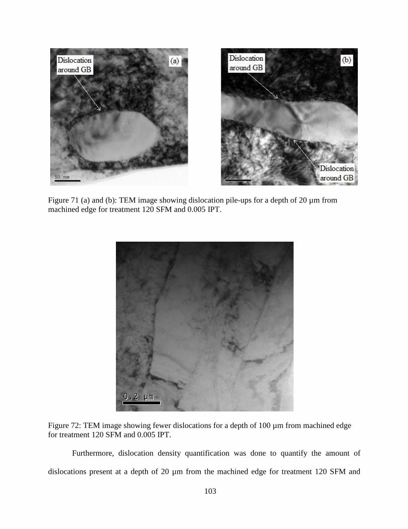
Figure 71 (a) and (b): TEM image showing dislocation pile-ups for a depth of 20 µm from machined edge for treatment 120 SFM and 0.005 IPT.
Figure 72: TEM image showing fewer dislocations for a depth of 100 µm from machined edge for treatment 120 SFM and 0.005 IPT.
Furthermore, dislocation density quantification was done to quantify the amount of
dislocations present at a depth of 20 µm from the machined edge for treatment 120 SFM and
103

0.005 IPR. Table 14 shows the si, ni and si2/ni
2 values. Figure 73 shows the graphical method
used to calculate the foil thickness (t) of the sample. The intercept of the line with the ordinate is
1/t2. Here, 1/t2 = 0.82 x 10⁻⁴ nm-2. Therefore, thickness of the foil (t) is 111 nm.
Table 14: CBED data for thickness determination.
Si (nm-1) ni Si
2/nk2 (nm-
2) 0.599 x 10⁻² 1 0.35 x 10⁻⁴ 1.7 x 10⁻² 2 0.72 x 10⁻⁴
Figure 73: Intercept plot to extrapolate foil thickness value.
After calculating the foil thickness, the dislocation density (ρ) was calculated by using
Eq. 3.
ρ = 1t (∑n𝑣∑𝐿v
+ ∑nℎ∑𝐿h
) (3)
where,
∑ nv = number of intersections of vertical test lines with the dislocations
∑ nh = number of intersections of horizontal test lines with the dislocations
∑ Lv = total length of vertical test lines
104

∑ Lh = total length of horizontal test lines
Five random sampling areas were selected on the two different images to calculate the
dislocation densities as shown in figures 74 (a) and (b). Both the images show a magnified inset
image with the approximate position where the grid was superimposed. Figure 75 shows the
individual and average dislocation densities for image 1 and 2. The literature does not report any
studies done to investigate the dislocation density by end milled American Iron and Steel
Institute (AISI) 1018 steel. The closest study reported was by Yeagashi Koh. Yeagashi, 2007
investigated before and after deformation dislocation density on manganese steels having 0.18%
carbon. The dislocation density (ρ) for the as-received material and material deformed in tension
at 0.2% /min was reported to be 6.1 x 10¹³ / m2 and 2.0 x 10¹⁴ / m2, respectively.
Figure 74 (a): TEM micrograph of image 1 used to determine ρ by the line intersection method at a depth of 20 µm from machined edge for treatment 120 SFM and 0.005 IPT.
105

Figure 74 (b): TEM micrograph of image 2 used to determine ρ by the line intersection method at a depth of 20 µm from machined edge for treatment 120 SFM and 0.005 IPT.
Figure 75: Dislocation density quantification at a depth of 20 µm from machined edge for treatment 120 SFM and 0.005 IPT.
Another closest study reported was by Yin et al. 2003. They investigated the dislocation
density for austenitized warm-rolled 1015 phosphorus steel; water quenched to avoid the
106
formation of pearlite microstructure in low carbon steel and reported a dislocation density (ρ) of
1.06 x 10¹⁴ / m2.
Some dislocation densities for low carbon steel as-received material reported in the
literature are 1.0 x 10⁶ / m2 for transformer steel having 0.005% carbon (Vorobev and Krivisha,
1971); 1.0 x 10⁶ / m2 for 0.9% carbon steel (Ryufuku, 2007) and 1.0 x 10¹² / m2 for Cr-Mn steel
having 0.06% carbon (Sternberk et al. 1985)
Other dislocation densities reported in the literature for low carbon steel after
deformation are 1.5 x 10¹⁴ / m2 for 0.05% carbon steel (Khodabakhshi and Kazeminezhad,
2011); 2.4 x 10¹³ / m2 for AISI 1035 steel (Mohandesi et al., 2007) and 1.0 x 10¹⁴ / m2 for AISI
4340 steel (Lee and Lam, 1996).
Increase in the dislocation density from the bulk of the material to the machined surface
can also be associated with the increase in strength of the material at the surface. This increase in
strength is already reported in this study. Taylor predicted that the strength of the metal crystal
(τ) obeys the following equation (Taylor, 1934)
τ = µ x b x α √ρ (4)
where,
µ = shear modulus = 80 GPa (for 1018 steel)
b = Burgers vector = 0.259 nm (for 1018 steel)
α = geometric constant = 0.5
ρ = dislocation density
If it is assumed that the average dislocation density (ρ) of the bulk of the material is 1.0 x
106 / m2. Than the shear strength of the bulk crystal (τbulk) will be 10,360 Pa or 1.50 Psi.
Similarly, if we calculate the shear strength of the machined crystal, considering the average
107

dislocation density 1.5 x 10⁹ / m2 from Image 1. Then the shear strength of the machined crystal
(τmachined) will be 401,241 Pa or 58.19 Psi. This shows that the increase in the strength of the
machined surface will be 38 times more than the bulk of the material. These results are in
agreement with the vickers hardness test conducted in this study.
EBSD Analysis
EBSD analysis was carried out on two-samples each, for the as-received sample and
samples at failure for the cutting speed and feed rate levels of (80 SFM – 0.003 IPT) and (120
SFM - 0.005 IPT), respectively. Figures 76 and 77 show the inverse pole figures (IPF) [001] of
all the phases, ferrite and iron carbide phases for the as-received material, respectively. Figures
78, 79, and 80 show the IPF of all the phases, ferrite phase and the iron carbide phase for sample
1 and 2 at failure when machining at the cutting speed and feed rate combination of 80 SFM and
0.003 IPT, respectively. Figures 81, 82 and 83 show the IPF of all the phases, ferrite phase and
iron carbide phase for sample 1 and 2 at failure when machining at the cutting speed and feed
rate combination of 120 SFM and 0.005 IPT, respectively. Samples 1 and 2 were taken from the
center and the edge of the machining cut on the workpiece, respectively.
108

Figure 76: IPF for all phases – As received material.
Figure 77: IPF for ferrite and iron carbide phase – As received material.
109

Figure 78: IPF for all phases – Sample 1 and 2 machined at 80 SFM and 0.003 IPT.
Figure 79: IPF for ferrite phase – Sample 1 and 2 machined at 80 SFM and 0.003 IPT.
110

Figure 80: IPF for iron carbide phase – Sample 1 and 2 machined at 80 SFM and 0.003 IPT.
Figure 81: IPF for all phases – Sample 1 and 2 machined at 120 SFM and 0.005 IPT.
111

Figure 82: IPF for ferrite phase – Sample 1 and 2 machined at 120 SFM and 0.005 IPT.
Figure 83: IPF for iron carbide phase – Sample 1 and 2 machined at 120 SFM and 0.005 IPT.
112

Figure 84 shows the grain size comparing between the as-received material and samples
at failure after machining at 80 SFM – 0.003 IPT and 120 SFM and 0.005 IPT.
Figure 84: Grain size comparison.
The grain size for the as-received sample obtained by using the American Society for
Testing and Materials (ASTM) method was 5 µm and by the EBSD was 2.47 µm. The observed
grain sizes for sample 1 and 2 for the cutting speed and feed rate combination of 80 SFM and
0.003 IPT were 13.2 µm and 9.54 µm, respectively. Similarly, the observed grain sizes for
sample 1 and 2 for the cutting speed and feed rate combination of 120 SFM and 0.005 IPT were
10.39 µm and 10.84 µm, respectively. The grain size distribution plot for the as- received
material, sample 1 for 80 SFM – 0.003 IPT and sample 1 for 120 SFM – 0.005 IPT is shown in
figures 85, 86 and 87, respectively. It was observed that there was some grain growth on the
machined surface. The grain growth was about 4 to 8 µm for both the cutting combination under
consideration. These grains cannot be associated with the grain growth mechanism which often
occurs after recrystallization since they do not have high enough temperature/time to reach the
113
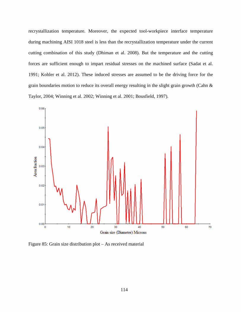
recrystallization temperature. Moreover, the expected tool-workpiece interface temperature
during machining AISI 1018 steel is less than the recrystallization temperature under the current
cutting combination of this study (Dhiman et al. 2008). But the temperature and the cutting
forces are sufficient enough to impart residual stresses on the machined surface (Sadat et al.
1991; Kohler et al. 2012). These induced stresses are assumed to be the driving force for the
grain boundaries motion to reduce its overall energy resulting in the slight grain growth (Cahn &
Taylor, 2004; Winning et al. 2002; Winning et al. 2001; Bousfield, 1997).
Figure 85: Grain size distribution plot – As received material
114

Figure 86: Grain size distribution plot for 80 SFM and 0.003 IPT – Sample 1
Figure 87: Grain size distribution plot for 120 SFM and 0.005 IPT – Sample 1
115

Also, the deformed machined surface is expected to have undergone the recovery
process/stage. Dislocations become mobile due to the materials stored energy. Recovery process
associated with plastic deformation is due to the annihilation of dislocations. Such annihilation
can occur by the coming together of dislocation segments of opposite sign. This type of recovery
process is called polygonization. In polygonization, gradual elimination of extraneous
dislocations and rearrangement of remaining dislocations occur, simultaneously. The sub-grain
formation is followed by sub-grain coarsening where the average grain size increases while the
number of sub-grain decreases (Doherty et al. 1997). Figure 88 show the ferrite pole figure for
the as-received material.
Figure 88: Ferrite pole figures – As received material.
It can be seen in figure 88, that the ferrite grains are moderately (001) textured along the
transverse direction (TD), while the (110) and (111) poles show no evidence of textured grains.
After machining it was observed that the ferrite maintained its c-axis texturing as seen in figure
89 and 90 for both the samples 1 and 2 at the cutting speed and feed rate combinations of (80
116

SFM – 0.003 IPT) and (120 SFM – 0.005 IPT), respectively. The iron carbide (Fe3C) pole
figures are not shown since the volume percent is too low to quantify texture.
Figure 89: Ferrite pole figures – Sample 1 and 2 machined at 80 SFM and 0.003 IPT.
Figure 90: Ferrite pole figures – Sample 1 and 2 machined at 120 SFM and 0.005 IPT.
117

CHAPTER 5
SUMMARY AND CONCLUSIONS
The focus of this present study was to investigate the effects of microlubrication during
end milling American Iron and Steel Institute (AISI) 1018 steel with a 1 inch solid carbide cutter
under varying cutting speed and feed rate levels and a constant depth of cut using Acculube 6000
vegetable based lubricant at a constant flow rate and air pressure of 12 ml/h and 0.1 MPa,
respectively. Machining experiments were carried out for a total of six combinations having
cutting speeds of 80, 100 and 120 surface feed per minute (SFM) and feed rates of 0.003 and
0.005 inches per revolution (IPT). The results were based on the multivariate analysis of variance
(MANOVA), parameter optimization, tool life, material removal rate (MRV), wear mechanisms,
cross sectional hardness measurements, transmission electron microscopy (TEM), scanning
electron microscopy (SEM) and electron backscattered diffraction (EBSD) analysis.
The MANOVA and analysis of variance (ANOVA) assumptions were found be robust.
The MANOVA model indicated that the main effects for the cutting speed and the feed rate
variables were significant. But, the interaction of (cutting speed*feed rate) was not significant at
95% confidence level.
The ANOVA for flank wear side 1 indicated that the cutting speed and feed rate variables
main effects were statistically significant while the interaction of (speed*feed) was not
statistically significant at 95% confidence level.
The ANOVA for flank wear side 2 indicated that the feed variable main effects is
statistically significant while the speed variables main effect and the interaction of (speed*feed)
are not statistically significant at 95% confidence level.
118

The ANOVA for aerosol mass concentration indicated that the feed rate variables main
effects was statistically significant while the cutting speed and the interaction of (speed*feed)
was not statistically significant at 95% confidence level.
The model was able to predict 69.44%, 68.06% and 42.90% of the variation in the data
for both the flank wear side 1, 2 and aerosol mass concentration, respectively. An adequate
signal-to-noise precision ratio of 9.54, 5.97 and 9.38 was obtained by the model for both the
flank wear side 1, 2 and aerosol mass concentration, respectively, indicating adequate signal
greater than 4. The model can therefore be used as a good predictor for both the flank wear sides
and aerosol mass concentration.
The parameter optimization was done by setting the goal to minimize flank wear Side 1,
Side 2 and aerosol mass concentration. It was observed that there was 84.2% desirability to
achieve a flank wear side 1 of 0.365 mm using a cutting speed of 120 SFM and 0.003 IPT. And
there was 60.7% desirability to achieve a flank wear side 2 of 0.380 mm using a cutting speed of
120 SFM and 0.0041 IPT. Also, there was 84.0% desirability to achieve a concentration of 5.91
mg/m3 using a cutting speed of 120 SFM and a feed rate of 0.005 IPT.
The highest average mass concentration of 8.32 mg/m3 was realized using treatment 80
SFM and 0.003 IPT. The lowest average mass concentration of 5.91 mg/m3 was realized using
treatment 120 SFM and 0.005 IPT. Atomization was dominant at low speed and feed rate while
vaporization/condensation mechanism was dominant at higher speed and feed rate combination.
Microlubrication generated low average mass concentration of aerosol for high feed rate
level of 0.005 IPT as compared to low feed rate level of 0.003 IPT. On the other hand,
microlubrication generated higher average particle size for lower speed rate levels as compared
to higher speed rate levels. During microlubrication, the main mechanism at work might be
119

cooling due to evaporation of the MWF. This points out towards developing MWF which have
higher latent heat of evaporation. Moreover, the aerosol concentrations during microlubrication
suggest the need for the scientific assessment of the atomization properties of MWFs. The
MWFs for microlubrication should be formulated in such a way that they atomize to a size range
that in non-hazardous to the environment and human health. It can be concluded that though
microlubrication may be effective in milling, more investigations should be carried out to lower
the mass concentration of the aerosol particles to below the recommended value of 5 mg/m3 by
Occupational Safety and Health Administration (OSHA) for mineral oil mist.
The cutting performance under microlubrication is five times better in terms of tool life
and two times better in terms of MRV under low cutting speed and feed rate combination (i.e. 80
SFM and 0.003 IPT) as compared to high cutting speed and feed rate combination (i.e. 120 SFM
and 0.005 IPT). The highest tool life of 861 minutes was realized using treatment 80 SFM and
0.003 IPT. Due to the lower cutting speed and feed rate the mist particle produced by
microlubrication easily penetrate through to the tool/workpiece interface promoting lubrication
and cooling. The lowest tool life of 21 minutes was realized using treatment 100 SFM and 0.005
IPT. Due to high feed rate, the cutting fluid is unable to effectively cool and lubricate the cutting
zone leading to higher temperatures and lower tool life.
All the cutting tools under consideration failed with gradual abrasive wear except for
treatment 80 SFM and 0.005 IPT, which underwent a catastrophic failure due to massive tool
chipping.
The treatments of (80 SFM – 0.003 IPT) and (120 SFM – 0.005 IPT) were further
considered for wear mechanisms analysis, cross sectional hardness measurements, SEM and
EBSD analysis. Based on SEM observation, two-body abrasion wear mode was likely dominant.
120

Other wear mechanisms were also active like sliding wear, adhesion and micro abrasion resulting
into micro fatigue crack, welded-micro chips and workpiece plowing.
Cross sectional hardness analyses indicated that the plastic deformation due to machining
extends to about 150 – 180 µm for both the treatments which was attributed to the increase in
dislocation density at the machined surface.
The surface profile of the workpiece suggested that for treatment 120 SFM and 0.005
IPT, 11% of the depth population (i.e. density of the distribution of the depth data points in the
profile) was in between 7.35 µm and 7.92 µm and for treatment 80 SFM and 0.003 IPT, 15% of
the depth population is in between 4.31 µm and 4.79 µm. The bearing area curve suggested that
for treatment 120 SFM and 0.005 IPT, almost 50% of the points have a depth that lies between 0
and 6.79 µm and for treatment 80 SFM and 0.003 IPT, almost 60% of the points have a depth
that lies between 0 and 4.79 µm. The Rq value for treatment 120 SFM and 0.005 IPT and
treatment 80 SFM and 0.003 IPT was 2.2 and 1.18 µm, respectively.
Cross sectional TEM analysis at failure was carried out for the cutting speed and feed rate
level of 120 SFM and 0.005 IPT to investigate the workpiece subsurface deformation and
strengthening. High concentration of dislocations were observed with an average dislocation
density (ρ) of 1.5 x 10⁹ / m2 for the sample taken at around 20 µm from machined edge, the
results were in accordance with cross sectional hardness measurements which showed high
hardness values near the surface and decreased hardness values while moving towards the bulk.
EBSD analysis showed a slight increase in grain size from the bulk for the both the
treatments. This was not due to the recrystallization process but due to the induced residual
stresses resulting in grain boundary motion. It was also observed that the ferrite maintained its
texture for both the treatments after machining.
121

Recommendation for Future Work
Future research for mist and microstructural analyses which can be done as an extension
to this study using the same material, process and parameters are:
1) Investigating the tool-workpiece interface temperature
2) Investigating the cutting forces generated during machining
3) Conducting a comparative study using dry, minimum quantity lubrication (MQL) and
flood coolant
4) Conducting a comparative study using different MQL flow rates
5) Conducting a comparative study using coated and uncoated tools
6) Investigating the effects of different vegetable oils
7) Conducting a surface roughness analysis
122
REFERENCES
ACGIH. (2001). Documentation of the threshold limits values and biological exposure indices. Sixth Edition, Cincinnati, American Conference of Governmental Industrial Hygienist.
Adler, D. P., Hii, W. W. S., Michalek, D. J., & Sutherland, J. W. (2006). Examining the role of
cutting fluid in machining and efforts to address associated environmental/health concerns. Machining Science and Technology, 10, 23-58.
American Society for Metals (ASM). (1990). Metals Handbook: Volume 1 – Properties and
Selection: Irons, Steels, and High-Performance Alloys, ASM International, Metals Park, OH.
Attanasio, A., Gelfi, M., Giardini, C., & Remino, C. (2006). Minimum quantity lubrication in
turning. Wear, 260, 333-338. Bennett, E. O., & Bennett, D. L. (1985). Occupational airways diseases in the metal working
industries. Tribology International, 18 (3), 169-176. Bhowmick, S., & Alpas, A. T. (2008). Minimum quantity lubrication drilling of aluminum-
silicon alloys in water using diamond-like carbon coated drills. International Journal of Machine Tools & Manufacture, 48, 1429-1443.
Boubekri, N., & Shaikh, V. (2012). Machining using minimum quantity lubrication: A
technology for sustainability. International Journal of Applied Science and Technology, 2, 111-115.
Bousfield, B. (1997). The metallography of deformation by material removal. Praktische
metallographie, 43 (1), 2-22. Bray, J. H., & Maxwell, S. E. (1985). Multivariate Analysis of Variance: Quantitative
applications in the social sciences, Second Edition, Sage Publications, Beverly Hills, CA. Brockhoff, T., & Walter, A. (1998). Fluid minimization in cutting and grinding, Abrasives,
October-November, 38-92. Cahn, J. W., & Taylor, J. E. (2004). A unified approach to motion of grain boundaries, relative
tangential translation along grain boundaries, and grain rotation. Acta Materialia, 52, 4887-4898.
Callister, W. D. Jr. (2007). Materials science and engineering: An introduction, Seventh Edition,
John and Wiley and Sons, New York City, NY. Chakraborty, P. (2008). Tool life and flank wear modeling of physical vapour deposited
TiAlN/TiN multilayer coated carbide end Mill inserts when machining 4340 steel under dry and semi-dry cutting conditions. University of Miami Scholarly Repository, Retrieved
123

from http://scholarlyrepository.miami.edu/cgi/viewcontent.cgi?article=1021&context= oa_dissertations
Chalmers, R. E. (1999). Global flavor highlights NAMRC XXVII. Manufacturing Engineering,
123 (1), 80-86. Childs, T. H.C., Maekawa, K., Obikawa, T., & Yamane, Y. (2000). Metal Machining - Theory
and Applications, Butterworth-Heinemann, Oxford, UK. Clarens, A. F., Zimmerman, J. B., Keoleian, G. A., Hayes, K. F., & Skerlos, S. J. (2008).
Comparison of life cycle emissions and energy consumption for environmentally adapted metalworking fluid systems. Environmental Science and Technology, 42 (22), 8534-8540.
Costa, E. S., Da Silva, M. B., & Machado, A. R. (2009). Burr produced on the drilling process as
a function of tool wear and lubricant coolant conditions. Journal of the Brazilian Society of Mechanical Science & Engineering, XXXI (1), 57-63.
Da Silva, R. B., Vieira, J. M., Cardoso, R. N., Carvalho, H. C., Costa, E. S., Machado, A. R., &
De Ávila, R. F. (2011). Tool wear analysis in milling of medium carbon steel with coated cemented carbide inserts using different machining lubrication/cooling systems. Wear, 271, 2459-2465.
Davis, J. R., (1989). Metals Handbook: Volume 16 – Machining, ASM International, Metals
Park, OH. Dhar, N. R., Ahmed, M. T., & Islam, S. (2006). An experimental investigation on effect of
minimum quantity lubrication in machining AISI 1040 steel. International Journal of Machine Tools and Manufacture, 47, 748-753.
Dhiman, S., Sehgal, R., Sharma, S. K., & Sharma, V. S. (2008). Machining behavior of AISI
1018 steel during turning. Journal of Scientific & Industrial Research, 67, 355-360. Doherty, R. D., Hughes, D. A., Humphreys, F. J., Jonas, J. J., Jensen, D. J., Kassner, M.
E., King, W. E., McNelley, T. R., McQueen, H. J., Rollett, A. D., (1997). Current issues in recrystallization: A review. Materials Science & Engineering A, A238 (2), 219-274.
Dosbaeva, J., Fox-Rabinovich, G., Dasch, J., & Veldhuis, S. (2008). Enhancement of wet and
MQL based machining of automotive alloys using cutting tools with DLC/Polymer surface treatments. Journal of Materials Engineering and Performance, 17 (3), 346-351.
Filipovic, A., & Stephenson, D. A. (2006). Minimum quantity lubrication (MQL) applications in
automotive power-train machining. Machining Science and Technology, 10, 3-22. Greaves, I. A., Eisen, E. A., Smith, T. J., Pothier, L. J., Kriebel, D., Woskie, S. R., Kennedy, S.
M., Shalat, S., & Monson, R. R., (1997). Respiratory health of automobile workers
124

exposed to metal-working fluid aerosols: respiratory symptoms. American Journal of Industrial Medicine, 32, 450-459.
Guhring Inc. (2012, September). Tool list. Retrieved from http://www.guhring.com/Documents
/Catalog/Tools/3146.pdf Hand, D. J., & Taylor, C. C. (1987). Multivariate Analysis of Variance and repeated measures:
A practical approach for behavioural scientist, Chapman and Hall Publishers, New York City, NY.
Hassan, A., & Yao, Z. (2005). Optimization of cutting parameters for face milling titanium alloy
using MQL. Journal of Donghua University, 22 (2), 9-12. Heisel, U., Schaal, M., & Wolf, G. (2009). Burr formation in milling with minimum quantity
lubrication. Production Engineering. Research and Development, 3, 23-30. Huynh, C. K. (2009). Occupational exposure to mineral oil metalworking fluid (MWFs) mist:
Development of new methodologies for mist sampling and analysis. Results from an Inter-laboratory Comparison. Journal of Physics: Conference Series, 151, 1-14.
Iqbal, A., Dar, N. U., He, N., Khan, I., & Li, L. (2008). Optimizing cutting parameter in
minimum quantity of lubrication milling of hardened cold work tool steel. Proceedings of the Institution of Mechanical Engineers, Part B, Journal of Engineering Manufacture, 223 (1), 43-54.
Iqbal, A., He, N., Khan, I., Liang, L., & Dar, N. U. (2008). Modeling the effects of cutting
parameters in MQL employed finish hard milling process using D-optimal method. Journal of Materials Processing Technology, 199, 379-390.
ITW Rocol North America. (September 2012). Acculube 6000 - Materials Safety Data Sheet.
Retrieved from http://www.itwfpg.com/TDS/acculube/lb6000.pdf Jayal, A. D., & Balaji, A. K. (2009). Effects of cutting fluid application on tool wear in
machining: Interactions with tool-coatings and tool surface features. Wear, 267, 1723-1730.
Jayal, A. D., Balaji, A. K., & Sesek, R. (2004). Environmentally conscious machining of a cast
aluminum alloys: Investigation of cutting fluid effects in drilling. Transaction of NAMRI/SME, 32, 415-422.
Jayal, A. D., Umbrello, D., Dillon, O. W., & Jawahir, I. S. (2010). An investigation of the effects
of cutting conditions, tool edge geometry, and workpiece hardness on surface integrity in orthogonal machining of AISI 52100 steel. Transaction of NAMRI/SME, 38, 57-64.
Kalpakjian, S. (1995). Manufacturing Engineering and Technology, Third Edition, Addison-
Wesley Publishing Company, Boston, MA.
125

Kang, M, C., Kim, K. H., Shin, S. H., Jang, S. H., Park, J. H., & Kim, C. (2008). Effect of the minimum quantity lubrication in high-speed end-milling of AISI D2 cold worked die steel (62 HRC) by coated carbide tools. Surface & Coatings Technology, 202, 5621-5624.
Khan, M. M. A., & Dhar, N. R. (2006). Performance evaluation of minimum quantity lubrication
by vegetable oil in terms of cutting force, cutting zone temperature, tool wear, job dimension and surface finish in turning AISI-1060 steel. Journal of Zhejiang University, Science A, 7 (11), 1790-1799.
Khan, M. M. A., Mithu, M. A. H., & Dhar, N. R. (2009). Effects of minimum quantity
lubrication on turning AISI 9310 alloy steel using vegetable oil-based cutting fluid. Journal of Materials Processing Technology, 209, 5573-5583.
Khodabakhshi, F., & Kazeminezhad, M. (2011). The effects of constrained groove pressing on
grain size, dislocation density and electrical resistivilty of low carbon steel. Materials and Design, 32, 3280-3285.
Köhler, J., Grove, T., Mai, O., & Denkena, B. (2012). Residual stresses in milled titanium parts.
Procedia CIRP, 2, 79-82. Kurgin, S., Barber, G., & Zou, Q. (2011). Cutting insert and work piece materials for minimum
quantity lubrication. Proceedings of the SPIE - The International Society for Optical Engineering, Fourth International Seminar on Modern Cutting and Measurement Engineering, 7997, 1-10.
Kwon, P. (2000). Predictive models for flank wear on coated inserts, Transaction of ASME, 122,
340-347. Lee, W., & Lam, H. (1996). The deformation behaviour and microstructure evolution of high-
strength alloy steel at high rate of strain. Journal of Materials Processing Technology, 57, 233-240.
Liao, Y. (February 2013). Foil thickness measurement. Practical electron microscopy and
database. Retrieved from http://www.globalsino.com/EM/page4832.html Meyveci, A., Karacan, I., Hanifi, F. E., Cahgulu, U., & Durmus, H. (2011). A study of wear and
aged aluminum alloys 2XXX and 6XXX within the MANOVA statistical analysis. Metal Science and Heat Treatment, 53 (3-4), 173-175.
Min, S., Inasaki, I., Fujimura, S., Wakabayashi, T & Suda, S. (2005). Investigation of adsorption
behaviour of lubricants in near-dry machining. Proceedings of the Institution of Mechanical Engineers, Part B: Journal of Engineering Manufacture, 219, 665-671.
Mohandesi, A, J., Rafiee, M, A., Maffi, O., & Saffarzadeh, P. (2007). Dependence of the yield
and fatigue strength of the thread rolled milled steel on dislocation density. Transaction of ASME, 129, 216-222.
126

Murakami, Y., & Yamamoto, T. (2007). Ecological deep hole drilling by novel coated and designed drill. Key Engineering Materials, 329, 657-662.
Northcott, W. H. (1868). A treatise on lathes and turning, simple, mechanical and ornamental.
Longmans Green and Company, London, UK. Olson, C. L. (1974). Comparative robustness of six tests in multivariate analysis of variance.
Journal of the American Statistical Association, 69, 894-908. Oxford Instruments. (March 2013). Electron Backscattered Diffraction. Retrieved from
www.ebsd.com Park, D. (2012). The occupational exposure limit for fluid aerosol generated in metalworking
operations: Limitations and recommendations. Safety and Health at Work, 3, 1-10. Rahman, M., Senthil, K. A., & Salam, M. U. (2002). Experimental evaluation on the effect of
minimal quantities of lubricant in milling, International Journal of Machine Tools & Manufacture, 42, 539-547.
Roy, A. K., Bandyopadhyay, S., Suresh, S. B., Maitra, D., Kumara, P., Wells, D., & Mac, L.
(2006). Relationship of residual stress to dislocation density in cold-worked martensitic alloy, Materials Science and Engineering A, 416, 134-138.
Ryu, S. H., Choi, D. K., & Chong, N. C., (2006). Roughness and texture generation on end
milled surface, International Journal of Machine Tools & manufacture, 46, 404-412. Ryufuku, S., Tomota, Y., Shiota, Y., Shiratori, T., Suzuki, H., & Moriai, A. (2007). Neutron
diffraction profile analysis to determine dislocation density and grain size for drawn steel wires. Materials Science Forum – Trans Tech Publications, 539, 2281-2286.
Sadat, A. B., Reddy, M. Y., & Wang, B. P. (1991). Plastic deformation analysis in machining of
Inconel-718 nickel-base superalloy using both experimental and numerical methods. Int. J. Mech. Sci., 33 (10), 829-842.
Sandvik Coromant. (2007). Application guide: Milling methods, 2D component features,
complete process solutions. AB Sandvikens Tryckeri, Sweden. Page: 29. Sanz, C., Fuentes, E., Gonzalo, O., Bengoetxea, I., Obermair, F., & Eidenhammer, M. (2008).
Advances in the ecological machining of magnesium and magnesium based hybrid parts. International Journal of Machining and Machinability of Materials, 4 (4), 302-319.
Shaikh, V., & Boubekri, N. (2010). Effects of minimum quantity lubrication in drilling 1018
steel, Journal of Manufacturing Technology Research, 2 (1/2), 1-14.
127

Sharif, S., Hisyam, M. A., & Kurniawan, D. (2009). Performance evaluation of vegetable oil as an alternative cutting lubricant when end milling stainless steel using TiAlN coated carbide tools. Transactions of NAMRI/SME, 37, 9-14.
Shaw, M., Pigott, J., & Richardson, L. (1951). The effect of cutting fluid upon chip-tool interface
temperature. Transaction of ASME, 73, 45-56. Sheehan, M. J. (1999). Final report of the OSHA metalworking fluids standard advisory
committee. OSHA Publications, 1-193. Shimadzu. (August 2012). Shimadzu Dynamic Ultra Micro Hardness Tester DUH-211/211S.
Retrieved from http://www.shimadzu.eu/brochure/DUH-211_211S.pdf Sreejith, P. S., & Ngoi, B. K. A. (2000). Dry machining: machining of the future. Journal of
Materials Processing Technology, 101, 287-291. Stachowiak, G. W., & Batchelor, A. W. (2005). Engineering Tribology, Third Edition, Elsevier
Inc, Oxford, UK. Sternberk, J., Kratochvilova, E., Gemperle, A., Faja, V., & Walder, V., (1985). Dependence of
characteristics of hysteresis loops on dislocation densities for low-alloy Cr-Mo steel. Czechoslovak Journal of Physics, 35 (11), 1259-1266.
Su, Y., He, N., Li. L., & Li, X. (2006). An experimental investigation of effects of
cooling/lubrication conditions on tool wear in high-speed end milling of Ti-6Al-4V. Wear, 261 (7-80, 760-766.
Sutherland, J. W., Kulur, V. N., & King, N. C. (2000). An experimental investigation of air
quality in wet and dry turning. Annals of the CIRP, 49 (1), 61-64. Taylor, F. W. (1906). On the art of cutting metals. The American Society of Mechanical
Engineers, New York City, NY. Taylor, G. I., (1934). The mechanism of plastic deformation of crystals. Part 1. Theoretical.
Proceedings of the Royal Society of London. Series A. 145 (855), 362-387. Thermo Scientific. (September 2012), Particulate Monitor DataRam4, Retrieved from
http://www.thermoscientific.com/ecomm/servlet/productsdetail_11152_L10955_89583_11961406_-1
U.S. Department of Health and Human Services. (1998). Occupational exposure to metal
working fluid. NIOSH Publication, 98-102. Vorobev, G, M., & Krivisha, L, V. (1971). X-Ray diffraction measurement of dislocation density
in transformer steel. Industrial Tribology, 37 (9), 1392-1395.
128

Wakabayashi, T., Inasaki, I., & Suda, S. (2006). Tribological action and optimal performance: Research activities regarding MQL machining fluids, Machining Science and Technology, 10, 59-85.
Weinert, K., Inasaki, I., Sutherland, J.W., & Wakabayashi, T. (2004). Dry machining and
minimum quantity lubrication. CIRP Ann. Manuf. Technol. 53, 511-537. William, D. B., & Carter, C. B. (2009). Transmission electron microscopy – A textbook for
materials science, Springer, New York City, NY. Winning, M., Gottstein, G., & Shvindlerman, L. S. (2002). On the mechanisms of grain
boundary migration. Acta Materialia, 50, 353-363. Winning, M., Gottstein, G., & Shvindlerman, L. S. (2001). Stress induced grain boundary
motion. Acta Materialia, 49, 211-219. Yan, L. T., Yuan, S. M., & Liu, Q. (2009). Effect of cutting parameters on minimum quantity
lubrication machining of high strength steel. Trans Tech Publications, Materials Science Forum, 626-627, 387-392.
Yeagashi, Koh. (2007). Dependence of magnetic susceptibility on dislocation density in tensile
deformed Iron and Mn-steel. ISIJ International, 47 (2), 327-332. Yanda, H., Ghani, J. A., Rodzi, M. N. A. M., Othman, K., & Haron, C. H. C. (2010).
Optimization of materials removal rate, surface roughness and tool life on conventional dry turning of FCD 700. International Journal of Mechanical and Materials Engineering (IJMME), 5 (2), 182-190.
Yin, F., Hanamura, T., Umezawa, O., & Nagai, K. (2003). Phosphorus-induced dislocation
structure variation in the warm rolled ultrafine-grained low-carbon steels. Materials Science and Engineering A, 354, 31-39.
Zhang, S., Li, J. F., & Wang, Y.W. (2012). Tool life and cutting forces in end milling Inconel
718 under dry and minimum quantity cooling lubrication cutting conditions. Journal of Cleaner Production, 32, 81-87.
Zhao, W., He, N., & Li. L. (2007). High speed milling of Ti6Al4V alloy with minimal quantity
lubrication. Key Engineering Materials, 329, 663-668.
129