CHAPTER V MODEL CALIBRATION AND VALIDATION

116

CHAPTER V

MODEL CALIBRATION AND VALIDATION

The current integrated hydrological model covers the sub-basin of Paya Indah fresh water

lakes and Kuala Langat Swamp Forest and their surroundings which are part of the regional

Langat River Basin. It is an integrated model including a suite of model components

simulating the flow on overland and in river/canals, flow in the unsaturated and saturated

zone, evapotranspiration losses to the atmosphere and an extension to describe the water

balance and its distribution.

The conjunctive use of surface water and groundwater requires a resource assessment

including both surface and subsurface domains. The calibration has consequently been

aimed at obtaining a satisfactory agreement for the simulated and observed groundwater

heads, surface water level and open-channel flow within the catchment.

Discontinuity in observation data as shown in some hydrographs of this thesis represent

some missing data due to some reading errors associated with the measuring devices.

117

Interpolation process was eliminated due to an occurrence of a remarkable discrepancy

between observed and simulated values. Following the calibration and validation of the

model, a sensitivity analysis was carried out to test how the model responds to variation of

certain parameters or input data.

5.1 CALIBRATION

The calibration process is primarily aiming at obtaining a set of model parameters, which

provide a satisfactory agreement between model results and field observations considering

the fact that calibration of distributed parameters is a complicated procedure.

In general there are mainly three categories of parameters that control the accuracy of

calibration process. These include: (1) the saturated hydraulic conductivity and the specific

yield of the aquifer of groundwater model and the model for water exchange between

aquifers and channels, (2) the infiltration and evapotranspiration rates which are used in the

2-layer water balance of unsaturated zone model, and (3) the Manning roughness

coefficient for overland grid cells and channel grid cells. The second group guarantees

correct simulation of the water yield volume. Parameters of this group are multipliers to

that are used in the infiltration and evapotranspiration models.

The Paya Indah wetland model was calibrated in three stages for the period of July 1st, 1999

to November 1st, 2004. This period was chosen because of availability of different

historical observation data which were required to achieve the calibration targets.

118

5.1.1 Calibration targets

In terms of water balance the ability of the model to simulate both wet and dry period

conditions is required. On the other hand problems of water table dropping in the shallow

aquifer and subsequently surface water at the Kuala Langat swamp Forest of the Paya Indah

hydrological system are only seen during dry period and associated with high water loss

due to the evapotranspiration which implies that low flows periods should be subjected to

special attention. The formulated calibration targets have been based on general criteria as

well as been tailored to the specific purpose of the Paya Indah wetland model and the

availability of field data. Subsequently, they should be seen as overall guidelines.

For the groundwater component of MIKE SHE, the objective first of all was a simulation of

the groundwater head at eight boreholes distributed across the modelled catchment; in

which observed data and simulation values were matched. This simulation helped in

calibrating the hydrological properties of the geological layers, i.e. horizontal and vertical

hydraulic conductivity. Furthermore, the range of potential head (maximum and minimum

levels) should be represented; and the model, to the extent possible, should be able describe

the full dynamics given limitations in input data.

The simulation water level of rivers and channels of the model were included as another

calibration target. The calibration locations included the North-Inlet-Canal (SWL1), Lakes’

system, and Lotus Lake Outlet (SWL2), in which all the simulated parameters matched

over the observed data.

119

In order to evaluate the model predictive capability, simulation of open-channel flow was

adopted for the inflow and outflow associated with the Paya Indah lakes system. The

North-Channel-Inlet (SWL1) and Lotus-outlet (SWL2) were considered as calibration

locations for inflow and outflow respectively.

5.1.2 Primary calibration parameters

The choice of calibration parameters was based on prior experience and a simple sensitivity

analysis. The number of calibration parameters is a key issue in the calibration procedure

and should be high enough to secure an optimal solution and full exploitation of the input

data and model complexity, but low enough to avoid over-parameterization and non-

uniqueness as well as excessive computation times (Refsgaard, 1997 “quoted” in Stisen et

al., 2008). The hydrological regime and thus the water balance of the Paya Indah wetland

are characterized by high rates of rainfall (2000 - 2300 mm/year) and evapotranspiration

(pan evaporation of 1100 - 1300 mm/year). The evapotranspiration is the dominant factor

of the water budget with or without considering artificial irrigation bearing in mind that the

catchment of Paya Indah wetland is characterized by rain-fed farming. The infiltration

capacity of the soils is high and the net rainfall seems to recharge the water table aquifer

noticeable at the area between Lotus Lake and Langat River. The flow in the water table

aquifer is in general directed towards the Langat River, unless there is no groundwater

abstraction taking place at the Megasteel Company’s property then the groundwater would

flow towards the discharging point. Due to the shallow groundwater table at peat layer (±1

m below ground surface) and furthermore occurrence of dense drainage and irrigation

canals network, a partial hydraulic contact between surface water bodies and the upper

120

aquifer sequence is more likely take place allowing lateral flow between the shallow

groundwater and the canals.

5.2 CALIBRATION RESULTS

The simulation of both surface water level and groundwater table provide a quite good

visual description of the hydrodynamic interaction at the modelled catchment of the Paya

Indah Wetland. Based on a visual qualitative assessment, a satisfactory performance was

attained at all the surface water and groundwater calibration points. However, noticeable

biases between observed measurements and simulated values were encountered causing

some overestimation as well as underestimation trends. Other than equipments errors, these

biases were mainly attributed to the unscheduled lock operations and over-abstraction of

groundwater that is carried out within the modelled catchment.

Distribution of different calibration locations were shown in Figures 1.3 and 4.21 for

surface water stage and discharge, and groundwater heads respectively.

5.2.1 Simulation of surface water level

The Paya Indah Wetland model was calibrated against surface water level at twelve

locations and the simulation results were shown in Figures 5.1-5.12. Results revealed that

drought conditions have caused the water level to drop between 20cm – 60cm.

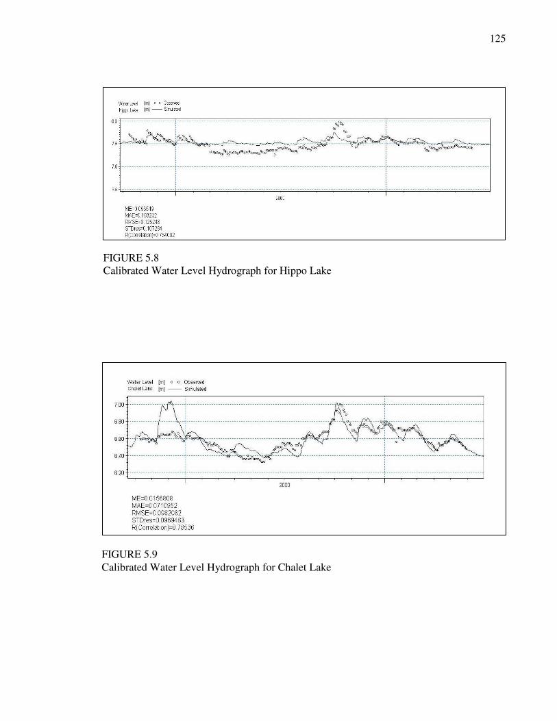
Good performance was obtained in nine calibration locations (Figures 5.1-5.9) in which

agreement between observed and simulated water levels were matched, with a correlation

(R) ≥0.75, during most of the calibration period. However, the observable overestimation or

121

underestimation trends that occurred only during short-time intervals were attributed to the

normal uncertainty associated with modelling; most possibly due to scaling problem.

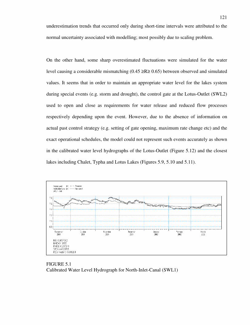
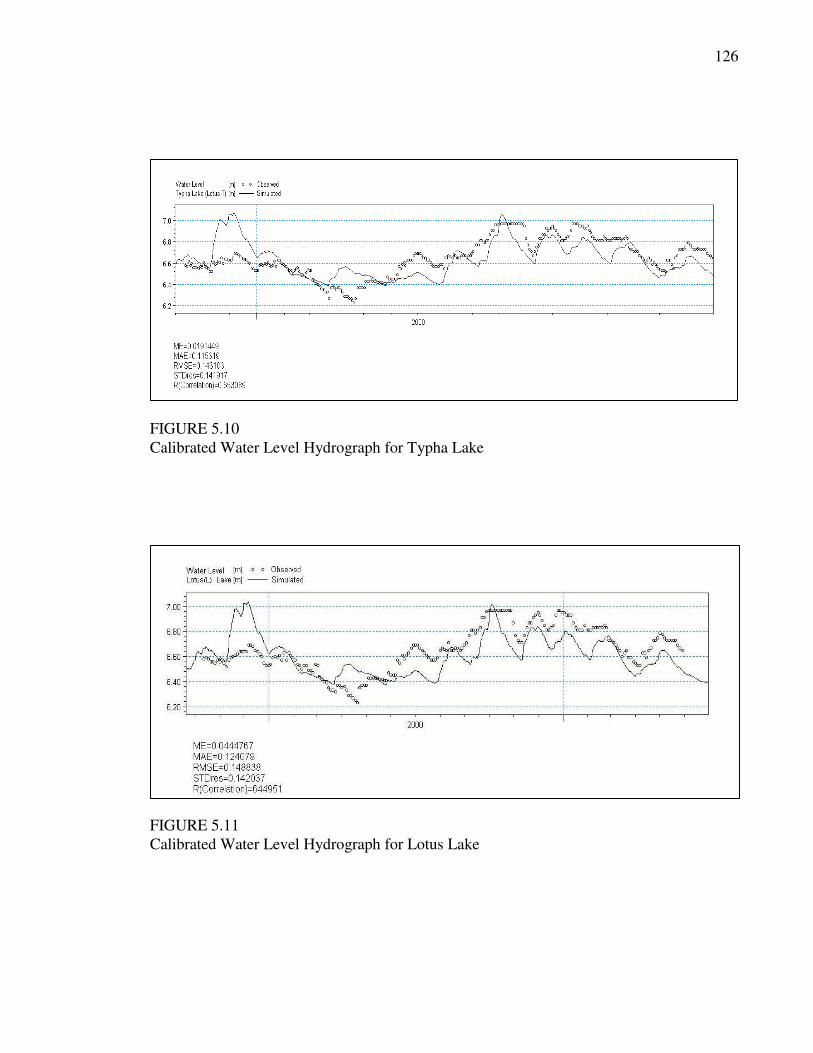
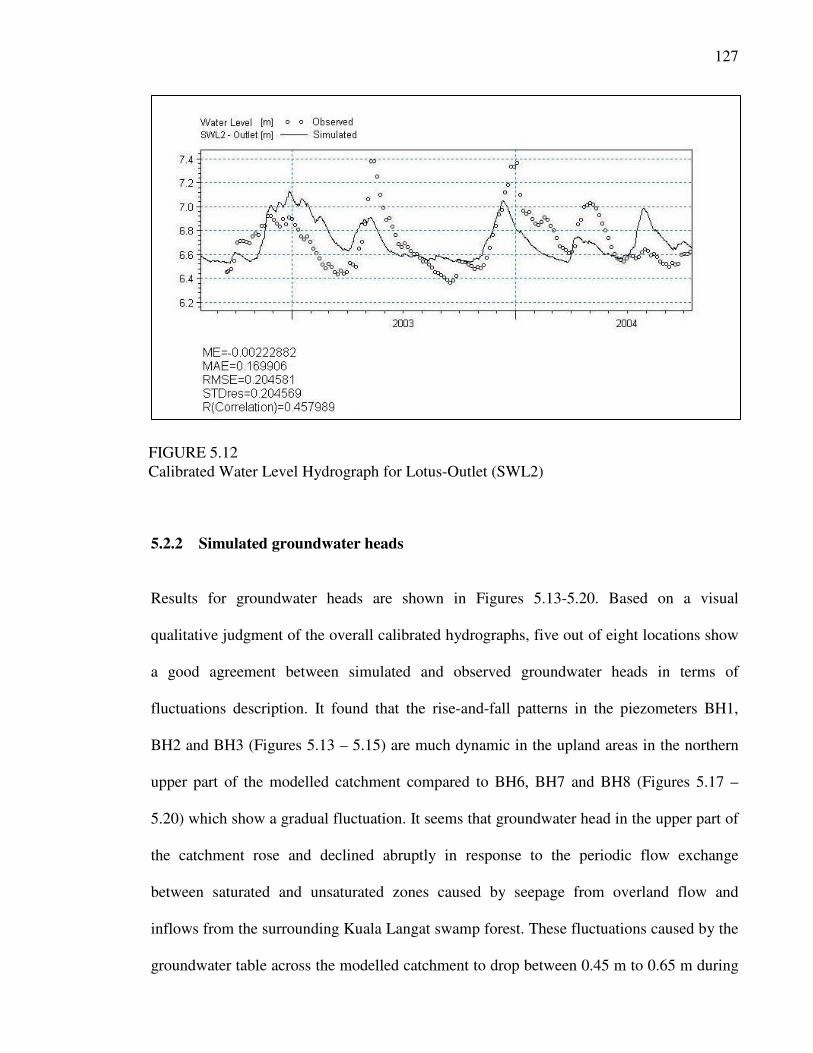
On the other hand, some sharp overestimated fluctuations were simulated for the water

level causing a considerable mismatching (0.45 ≥R≥ 0.65) between observed and simulated

values. It seems that in order to maintain an appropriate water level for the lakes system

during special events (e.g. storm and drought), the control gate at the Lotus-Outlet (SWL2)

used to open and close as requirements for water release and reduced flow processes

respectively depending upon the event. However, due to the absence of information on

actual past control strategy (e.g. setting of gate opening, maximum rate change etc) and the

exact operational schedules, the model could not represent such events accurately as shown

in the calibrated water level hydrographs of the Lotus-Outlet (Figure 5.12) and the closest

lakes including Chalet, Typha and Lotus Lakes (Figures 5.9, 5.10 and 5.11).

FIGURE 5.1

Calibrated Water Level Hydrograph for North-Inlet-Canal (SWL1)

122

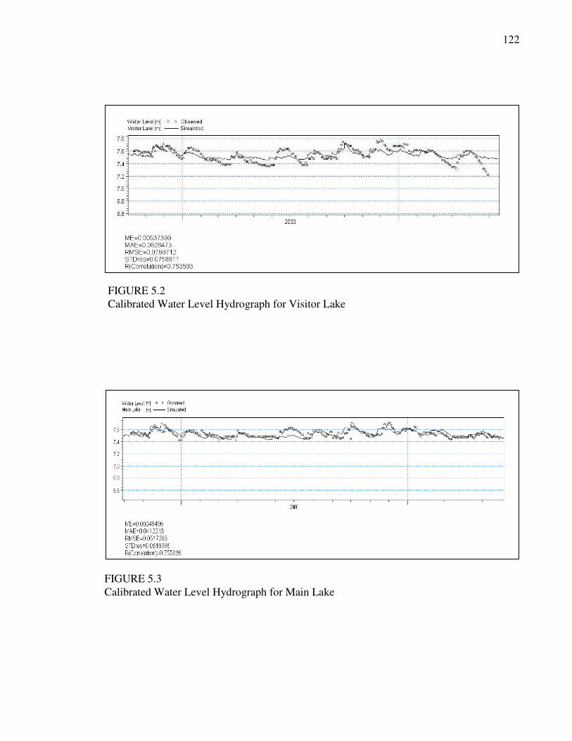
FIGURE 5.2

Calibrated Water Level Hydrograph for Visitor Lake

FIGURE 5.3

Calibrated Water Level Hydrograph for Main Lake

123

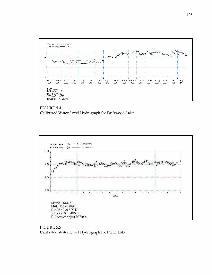
FIGURE 5.4

Calibrated Water Level Hydrograph for Driftwood Lake

FIGURE 5.5

Calibrated Water Level Hydrograph for Perch Lake

124

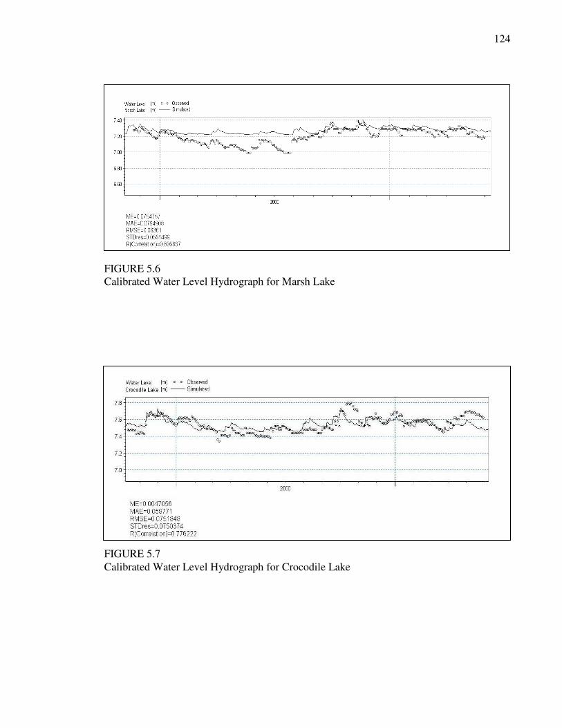
FIGURE 5.6

Calibrated Water Level Hydrograph for Marsh Lake

FIGURE 5.7

Calibrated Water Level Hydrograph for Crocodile Lake

125

FIGURE 5.8

Calibrated Water Level Hydrograph for Hippo Lake

FIGURE 5.9

Calibrated Water Level Hydrograph for Chalet Lake

126

FIGURE 5.10

Calibrated Water Level Hydrograph for Typha Lake

FIGURE 5.11

Calibrated Water Level Hydrograph for Lotus Lake

127

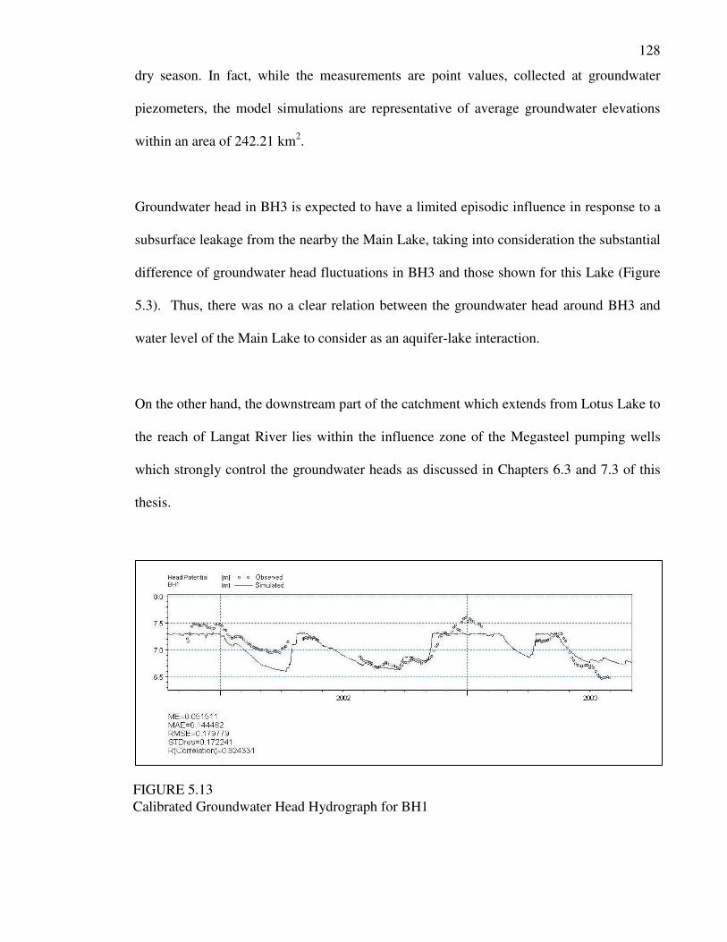
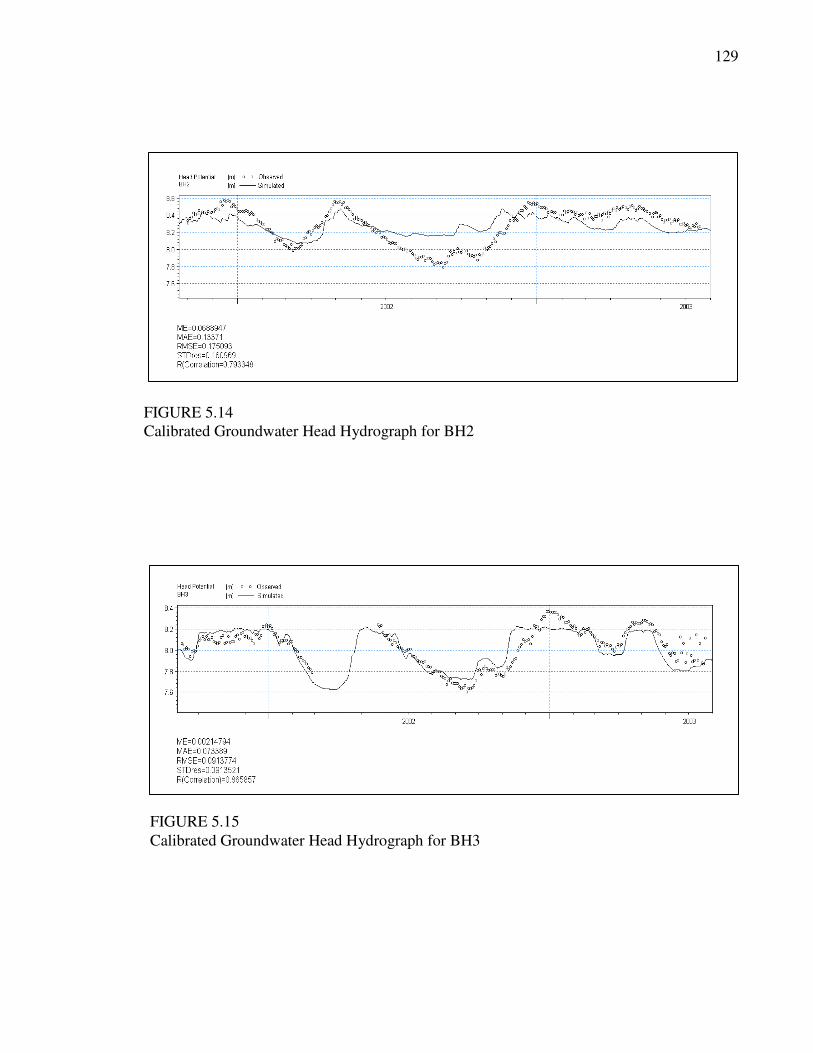
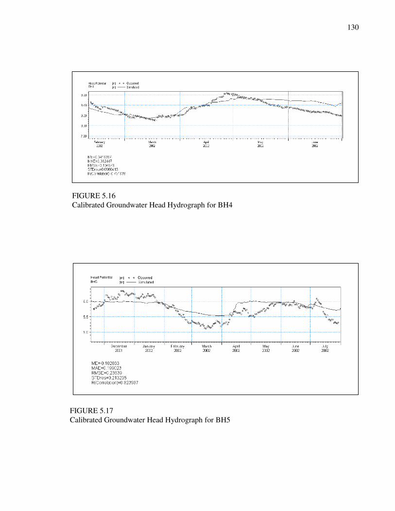
5.2.2 Simulated groundwater heads

Results for groundwater heads are shown in Figures 5.13-5.20. Based on a visual

qualitative judgment of the overall calibrated hydrographs, five out of eight locations show

a good agreement between simulated and observed groundwater heads in terms of

fluctuations description. It found that the rise-and-fall patterns in the piezometers BH1,

BH2 and BH3 (Figures 5.13 – 5.15) are much dynamic in the upland areas in the northern

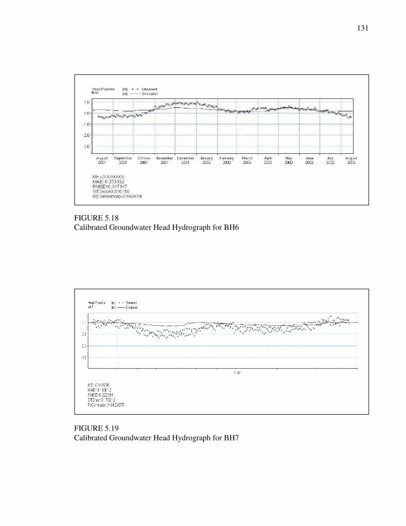
upper part of the modelled catchment compared to BH6, BH7 and BH8 (Figures 5.17 –

5.20) which show a gradual fluctuation. It seems that groundwater head in the upper part of

the catchment rose and declined abruptly in response to the periodic flow exchange

between saturated and unsaturated zones caused by seepage from overland flow and

inflows from the surrounding Kuala Langat swamp forest. These fluctuations caused by the

groundwater table across the modelled catchment to drop between 0.45 m to 0.65 m during

FIGURE 5.12

Calibrated Water Level Hydrograph for Lotus-Outlet (SWL2)

128

dry season. In fact, while the measurements are point values, collected at groundwater

piezometers, the model simulations are representative of average groundwater elevations

within an area of 242.21 km2.

Groundwater head in BH3 is expected to have a limited episodic influence in response to a

subsurface leakage from the nearby the Main Lake, taking into consideration the substantial

difference of groundwater head fluctuations in BH3 and those shown for this Lake (Figure

5.3). Thus, there was no a clear relation between the groundwater head around BH3 and

water level of the Main Lake to consider as an aquifer-lake interaction.

On the other hand, the downstream part of the catchment which extends from Lotus Lake to

the reach of Langat River lies within the influence zone of the Megasteel pumping wells

which strongly control the groundwater heads as discussed in Chapters 6.3 and 7.3 of this

thesis.

FIGURE 5.13

Calibrated Groundwater Head Hydrograph for BH1

129

FIGURE 5.14


FIGURE 5.15


130

FIGURE 5.16


FIGURE 5.17


131

FIGURE 5.18


FIGURE 5.19


132

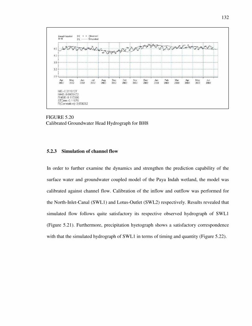
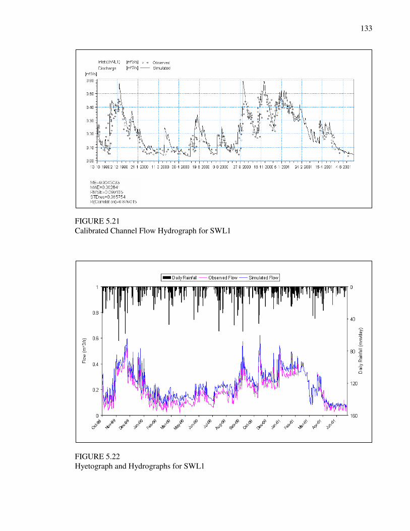
5.2.3 Simulation of channel flow

In order to further examine the dynamics and strengthen the prediction capability of the

surface water and groundwater coupled model of the Paya Indah wetland, the model was

calibrated against channel flow. Calibration of the inflow and outflow was performed for

the North-Inlet-Canal (SWL1) and Lotus-Outlet (SWL2) respectively. Results revealed that

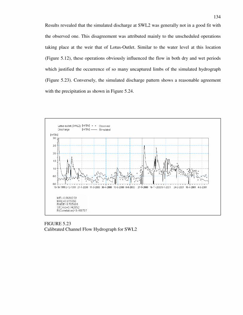
simulated flow follows quite satisfactory its respective observed hydrograph of SWL1

(Figure 5.21). Furthermore, precipitation hyetograph shows a satisfactory correspondence

with that the simulated hydrograph of SWL1 in terms of timing and quantity (Figure 5.22).

FIGURE 5.20


133

FIGURE 5.21

Calibrated Channel Flow Hydrograph for SWL1

FIGURE 5.22

Hyetograph and Hydrographs for SWL1

134

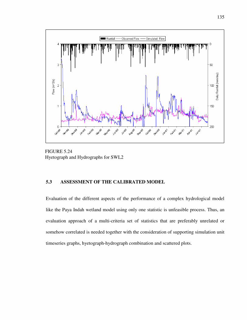
Results revealed that the simulated discharge at SWL2 was generally not in a good fit with

the observed one. This disagreement was attributed mainly to the unscheduled operations

taking place at the weir that of Lotus-Outlet. Similar to the water level at this location

(Figure 5.12), these operations obviously influenced the flow in both dry and wet periods

which justified the occurrence of so many uncaptured limbs of the simulated hydrograph

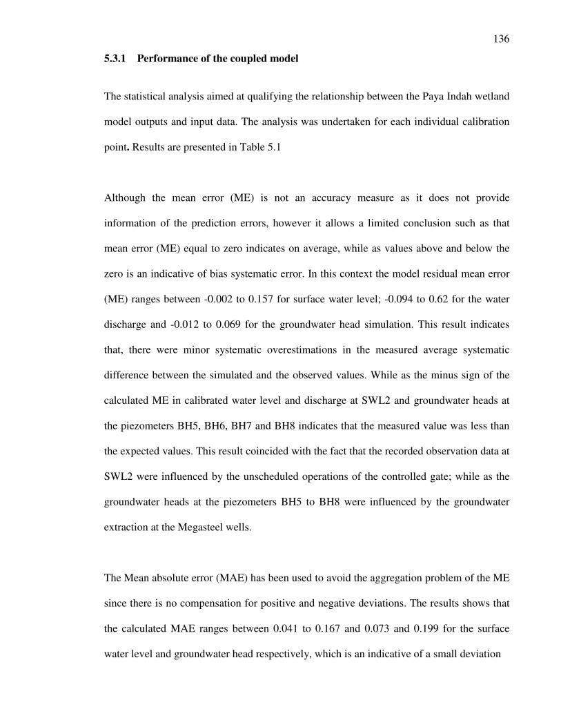
(Figure 5.23). Conversely, the simulated discharge pattern shows a reasonable agreement

with the precipitation as shown in Figure 5.24.

FIGURE 5.23

Calibrated Channel Flow Hydrograph for SWL2

135

FIGURE 5.24

Hyetograph and Hydrographs for SWL2

5.3 ASSESSMENT OF THE CALIBRATED MODEL

Evaluation of the different aspects of the performance of a complex hydrological model

like the Paya Indah wetland model using only one statistic is unfeasible process. Thus, an

evaluation approach of a multi-criteria set of statistics that are preferably unrelated or

somehow correlated is needed together with the consideration of supporting simulation unit

timeseries graphs, hyetograph-hydrograph combination and scattered plots.

136

5.3.1 Performance of the coupled model

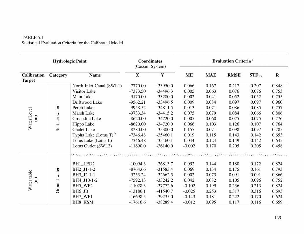
The statistical analysis aimed at qualifying the relationship between the Paya Indah wetland

model outputs and input data. The analysis was undertaken for each individual calibration

point. Results are presented in Table 5.1

Although the mean error (ME) is not an accuracy measure as it does not provide

information of the prediction errors, however it allows a limited conclusion such as that

mean error (ME) equal to zero indicates on average, while as values above and below the

zero is an indicative of bias systematic error. In this context the model residual mean error

(ME) ranges between -0.002 to 0.157 for surface water level; -0.094 to 0.62 for the water

discharge and -0.012 to 0.069 for the groundwater head simulation. This result indicates

that, there were minor systematic overestimations in the measured average systematic

difference between the simulated and the observed values. While as the minus sign of the

calculated ME in calibrated water level and discharge at SWL2 and groundwater heads at

the piezometers BH5, BH6, BH7 and BH8 indicates that the measured value was less than

the expected values. This result coincided with the fact that the recorded observation data at

SWL2 were influenced by the unscheduled operations of the controlled gate; while as the

groundwater heads at the piezometers BH5 to BH8 were influenced by the groundwater

extraction at the Megasteel wells.

The Mean absolute error (MAE) has been used to avoid the aggregation problem of the ME

since there is no compensation for positive and negative deviations. The results shows that

the calculated MAE ranges between 0.041 to 0.167 and 0.073 and 0.199 for the surface

water level and groundwater head respectively, which is an indicative of a small deviation

137

between the observed and simulated data. Conversely, the highest MAE value of 0.92

which was calculated for the discharge at SWL2 indicates relatively a large deviation

between simulation and prediction values.

Unlike the mean absolute error (MAE), the root mean square error (RMSE) is highly

sensitive in terms of assessing large errors, thus provides a better judgment. In this concern

the calculated RMSE varied between 0.052 to 0.217, and 0.091 to 0.317 for surface water

and groundwater levels respectively. Despite the considerable biases between observed and

simulated hydrographs of the SWL2 resulted in a relatively large RMSE value of 0.77,

these results revealed that the vertical distance of the observed data from the fitted line of

the model parameters is very narrow which in turn, demonstrates that the average random

discrepancies between simulations and observations were small.

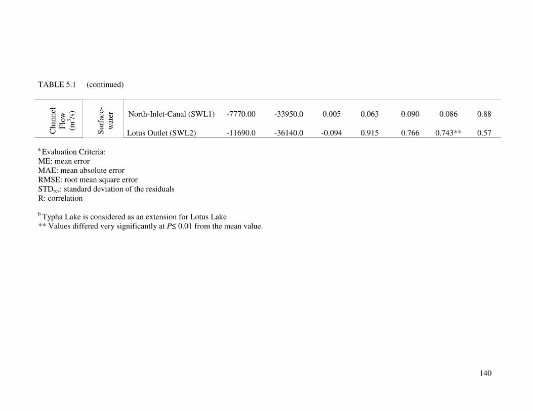
With the exception to SWL2 data in which observed and simulated flow values deviate a

significant volume (P ≤ 0.01) of 0.74 m3/s from its mean value; the overall low standard

deviation values which were calculated for the whole calibrated hydrographs indicate a

satisfactory prediction accuracy of the model. Furthermore, this result was further

strengthened by the Pearson distribution index (R2) and coefficient of efficiency (CE)

which were calculated for the channel flow.

The values of the coefficients of correlation (R) varied widely among the different

calibrated categories. Values that were obtained for the surface water level and discharge

range from 0.46 to 0.96 and 0.47 to 0.86 respectively. While as the groundwater head

obtained values range from 0.62 to 0.87. The strong correlation values calculated for the

majority of the simulated points indicate good one-to-one match between the measured and

138

simulated values. However, the relatively low correlation coefficient values of both stage

(0.46) and discharge (0.47) at SWL2 and the moderate correlation coefficient values of

0.645 and 0.653 for Lotus and Typha lakes respectively, were attributed mainly to the bias

of operations of unscheduled water release and control at the Lotus Outlet controlled gate

which influenced both the water stage and discharge. On the other hand the low correlation

coefficient value of 0.62 for BH7 and the moderate correlation coefficient values of 0.65

and 0.69 for both BH8 and BH6 respectively indicate the influence of over-extraction and

irregular withdrawal rate of groundwater that is carried out by the Megasteel Co. Ltd. on

that part of the modelled catchment.

139

TABLE 5.1

Statistical Evaluation Criteria for the Calibrated Model

Hydrologic Point

Coordinates

(Cassini System)

Evaluation Criteria

a

Calibration

Target

Category Name X Y ME MAE RMSE STDres R

Wat

er L

evel

(m)

Su

rfac

e-w

ater

North-Inlet-Canal (SWL1) -7770.00 -33950.0 0.066 0.167 0.217 0.207 0.848

Visitor Lake -7373.50 -34496.3 0.005 0.063 0.076 0.076 0.753

Main Lake -9170.00 -33280.0 0.002 0.041 0.052 0.052 0.755

Driftwood Lake -9562.21 -33496.5 0.009 0.084 0.097 0.097 0.960

Perch Lake -9958.52 -34811.5 0.013 0.071 0.086 0.085 0.757

Marsh Lake -9733.34 -34415.2 0.075 0.079 0.084 0.066 0.806

Crocodile Lake -8620.00 -34720.0 0.005 0.060 0.075 0.075 0.776

Hippo Lake -8620.00 -34720.0 0.066 0.103 0.126 0.107 0.764

Chalet Lake -8280.00 -35300.0 0.157 0.071 0.098 0.097 0.785

Typha Lake (Lotus T) b

-7346.48 -35460.1 0.019 0.115 0.143 0.142 0.653

Lotus Lake (Lotus L) -7346.48 -35460.1 0.044 0.124 0.149 0.142 0.645

Lotus Outlet (SWL2) -11690.0 -36140.0 -0.002 0.170 0.205 0.205 0.458

Wat

er t

able

(m)

Gro

un

d-w

ater

BH1_LED2 -10094.3 -26813.7

0.052

0.144

0.180

0.172

0.824

BH2_J1-1-2 -8764.66 -31583.4 0.069 0.134 0.175 0.161 0.793

BH3_J2-1-1 -9253.24 -32662.5 0.002 0.073 0.091 0.091 0.866

BH4_J10-1-2 -7592.13 -33242.2 0.042 0.082 0.105 0.096 0.752

BH5_WF2 -11028.3 -37772.6 -0.102 0.199 0.236 0.213 0.824

BH6_JB -13186.1 -41540.7 -0.025 0.253 0.317 0.316 0.693

BH7_WF1 -16698.5 -39235.0 -0.143 0.181 0.222 0.170 0.624

BH8_KSM -17616.6 -38289.4 -0.012 0.095 0.117 0.116 0.659

139

140

TABLE 5.1 (continued)

a Evaluation Criteria:

ME: mean error

MAE: mean absolute error

RMSE: root mean square error

STDres: standard deviation of the residuals

R: correlation

b Typha Lake is considered as an extension for Lotus Lake

** Values differed very significantly at P≤ 0.01 from the mean value.

Ch

ann

el

Flo

w

(m3/s

)

Su

rfac

e-

wat

er

North-Inlet-Canal (SWL1)

-7770.00

-33950.0

0.005

0.063

0.090

0.086

0.88

Lotus Outlet (SWL2) -11690.0 -36140.0 -0.094 0.915 0.766 0.743** 0.57

140

141

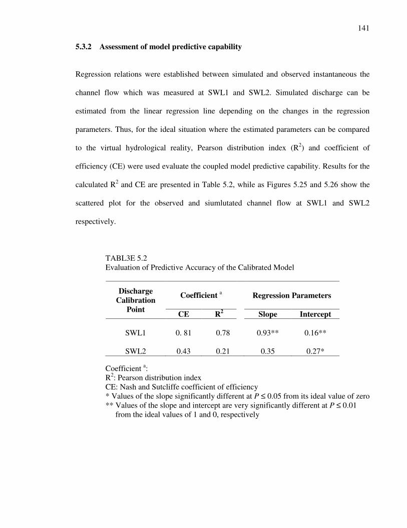
5.3.2 Assessment of model predictive capability

Regression relations were established between simulated and observed instantaneous the

channel flow which was measured at SWL1 and SWL2. Simulated discharge can be

estimated from the linear regression line depending on the changes in the regression

parameters. Thus, for the ideal situation where the estimated parameters can be compared

to the virtual hydrological reality, Pearson distribution index (R2) and coefficient of

efficiency (CE) were used evaluate the coupled model predictive capability. Results for the

calculated R2 and CE are presented in Table 5.2, while as Figures 5.25 and 5.26 show the

scattered plot for the observed and siumlutated channel flow at SWL1 and SWL2

respectively.

TABL3E 5.2

Evaluation of Predictive Accuracy of the Calibrated Model

Discharge

Calibration

Point

Coefficient a

Regression Parameters

CE R2

Slope Intercept

SWL1 0. 81 0.78 0.93** 0.16**

SWL2

0.43

0.21

0.35

0.27*

Coefficient a:

R2: Pearson distribution index

CE: Nash and Sutcliffe coefficient of efficiency

* Values of the slope significantly different at P ≤ 0.05 from its ideal value of zero

** Values of the slope and intercept are very significantly different at P ≤ 0.01

from the ideal values of 1 and 0, respectively

142

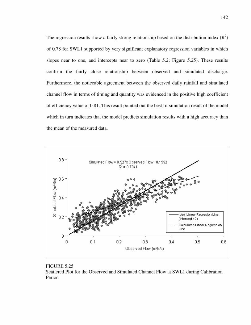
The regression results show a fairly strong relationship based on the distribution index (R2)

of 0.78 for SWL1 supported by very significant explanatory regression variables in which

slopes near to one, and intercepts near to zero (Table 5.2; Figure 5.25). These results

confirm the fairly close relationship between observed and simulated discharge.

Furthermore, the noticeable agreement between the observed daily rainfall and simulated

channel flow in terms of timing and quantity was evidenced in the positive high coefficient

of efficiency value of 0.81. This result pointed out the best fit simulation result of the model

which in turn indicates that the model predicts simulation results with a high accuracy than

the mean of the measured data.

FIGURE 5.25

Scattered Plot for the Observed and Simulated Channel Flow at SWL1 during Calibration Period

143

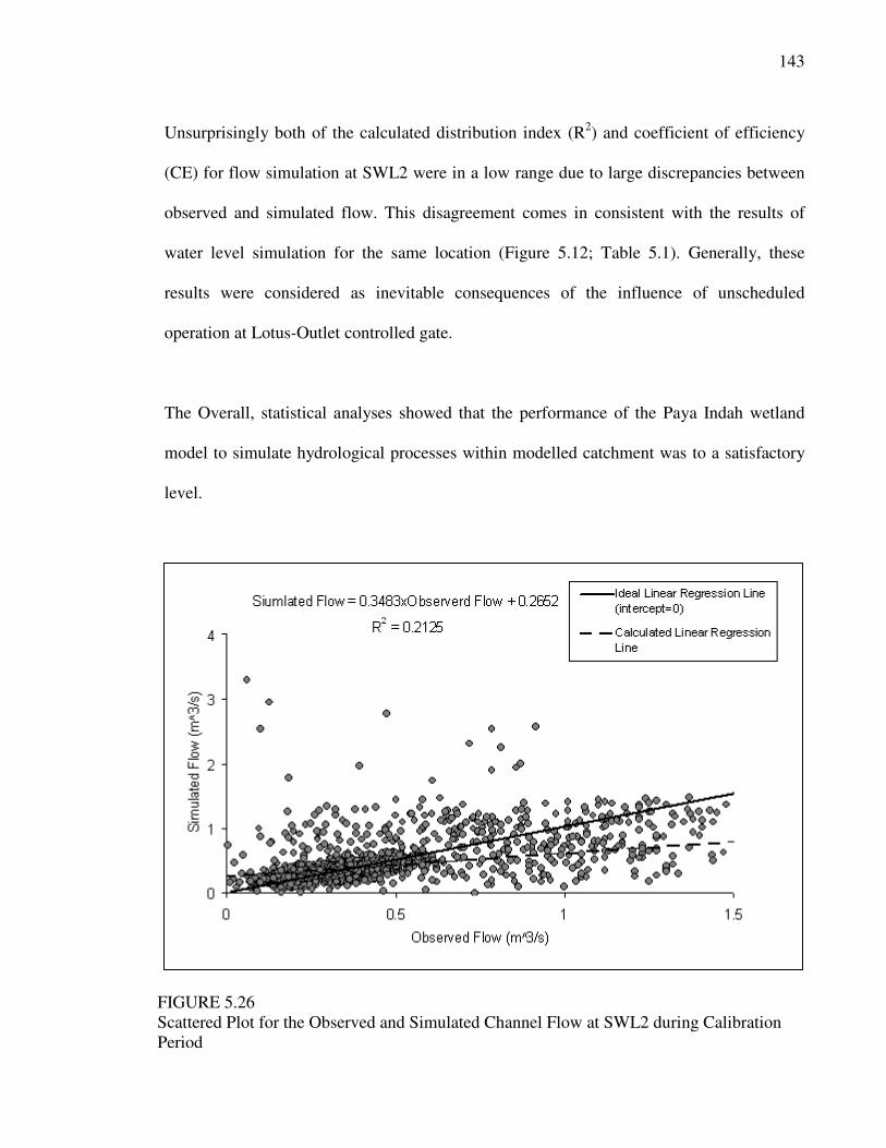
Unsurprisingly both of the calculated distribution index (R2) and coefficient of efficiency

(CE) for flow simulation at SWL2 were in a low range due to large discrepancies between

observed and simulated flow. This disagreement comes in consistent with the results of

water level simulation for the same location (Figure 5.12; Table 5.1). Generally, these

results were considered as inevitable consequences of the influence of unscheduled

operation at Lotus-Outlet controlled gate.

The Overall, statistical analyses showed that the performance of the Paya Indah wetland

model to simulate hydrological processes within modelled catchment was to a satisfactory

level.

FIGURE 5.26

Scattered Plot for the Observed and Simulated Channel Flow at SWL2 during Calibration

Period

144

5.4 VALIDATION

A distributed hydrological model can be considered validated not only if it is able to

produce good simulations for future conditions, but also if it is able to perform reliable

predictions at internal/multi-site locations (Refsgaard, 1997). On this context, the

performance of the calibrated model was validated for one year using present data. The period

from August 2007 to August 2008 was chosen for the model validation in order to cover one

full hdrologic year. All parameters applied in the calibration are unchanged during

validation. The validation of the model was aimed at investigating the reliability of model

parameters which were applied for the calibration period (July 1999 - November 2004) in

order to simulate the ongoing land use change in the Paya Indah wetland catchment. The

canal network and groundwater wells locations are assumed identical for the calibration

period implying that the canal system, but not necessarily the water flow and level, is

unchanged.

Due to vandalism problem which was discussed in Chapter 4.7of this thesis, the validation

process was confined to eight locations for the surface water level, two locations for

groundwater heads, and two locations for channel flow excluding the North-Canal-Inlet

(SWL1) where the automatic logger was smashed.

145

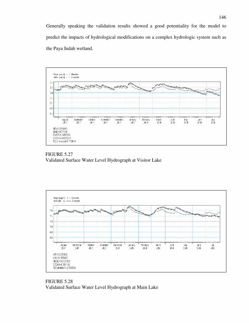
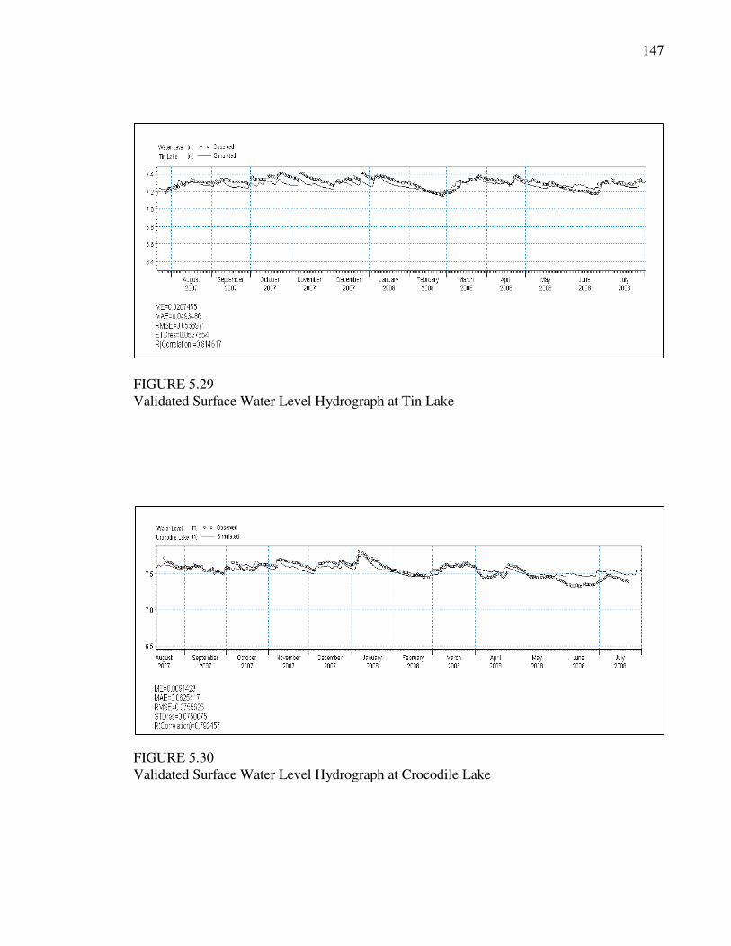
5.4.1 Validated surface water flow

Surface water level was validated at eight different locations including Visitor, Main, Tin,

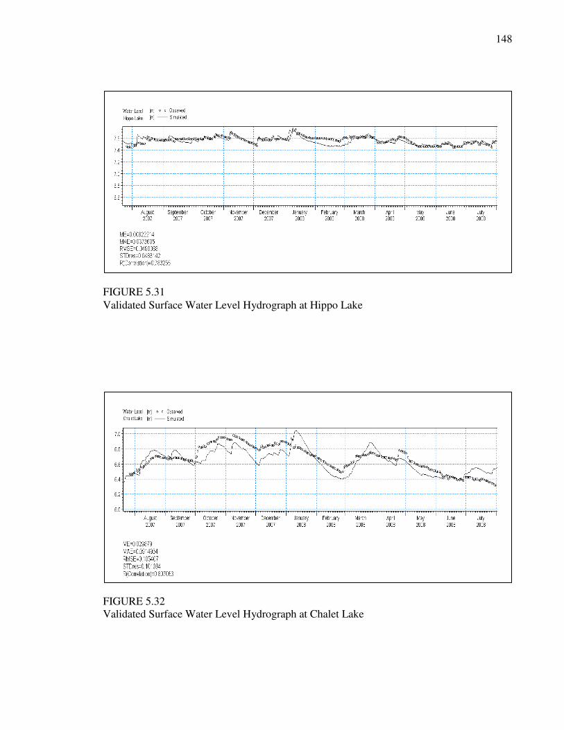
Crocodile, Hippo, Chalet, Typha and Lotus lakes. Figures 5.27 – 5.34 illustrate observed

and simulated water level hydrographs. The results clearly revealed that the validated

model response was much better than the calibrated model. Despite the short-term running

of the validation period, it was found that the dynamics of the water level was well

represented by the validated model. Furthermore most of the simulated flow peaks matched

well with their observed counterparts especially for the upper and middle lakes (Figures

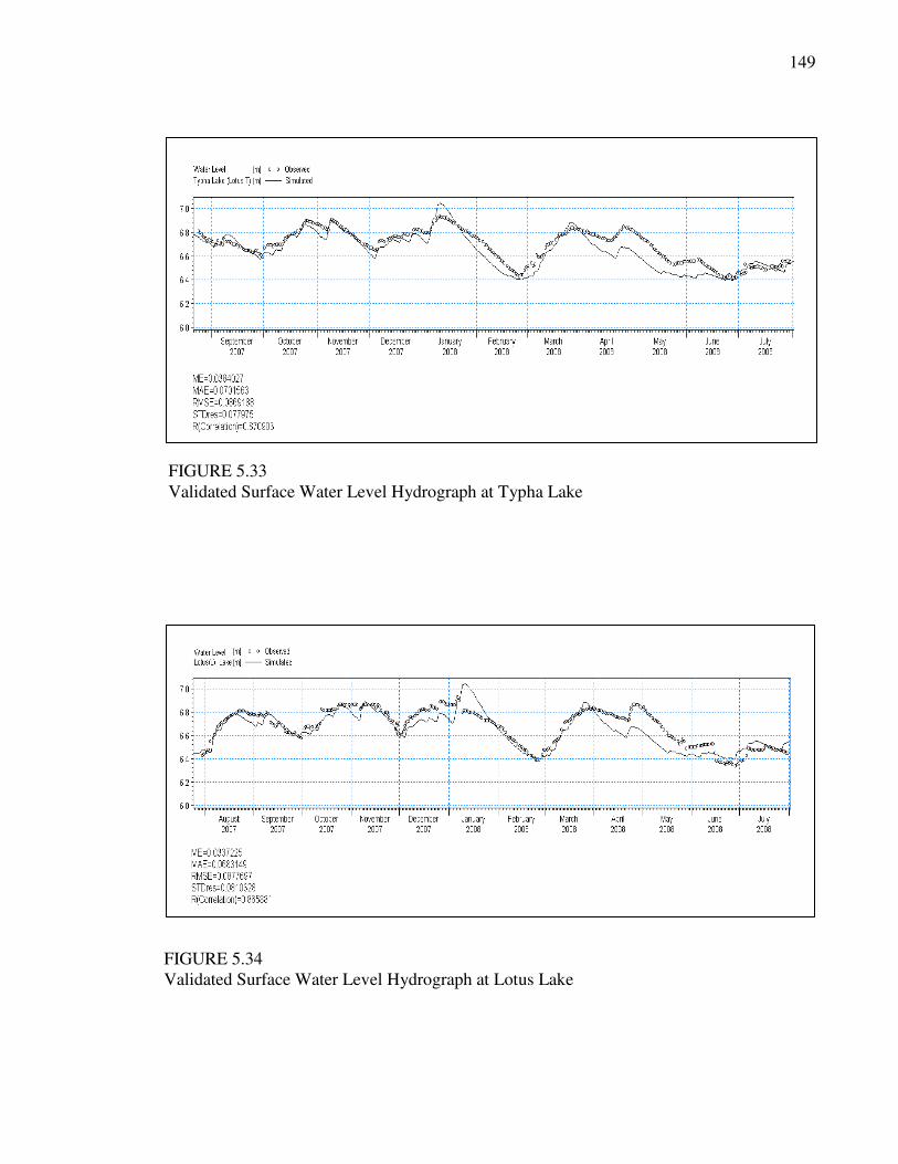
5.27 to 5.31). However at the lower lakes, mainly Chalet, Typha and Lotus, it seems that

the model missed capturing two anomalous peaks that were occurred during the periods 04

- 11 January 2008 and 22 – 25 March 2008 i.e. occurred after certain events (Figures 5.32

to 5.35). These anomalies were justified by the occurrence of four and two successive

storms during the first and second periods respectively which in turn represented 8.2% and

3.2% of the total rainfall during the whole validation period.

On the other hand, based on an information tip from the local authorities there were no

operations for the SWL2 control gate during the whole validation period. This action may

explain the good representation of the surface water dynamics characteristics during the

validation period rather than the calibration one. Thus the slightly overall under-estimation

especially lower lakes, was mainly related to the fact that the accumulation of water in the

Lotus lake after storm events tends to exceed the discharge intake capacity of the broad-

crested weirs type of the controlled gate.

146

Generally speaking the validation results showed a good potentiality for the model to

predict the impacts of hydrological modifications on a complex hydrologic system such as

the Paya Indah wetland.

FIGURE 5.27

Validated Surface Water Level Hydrograph at Visitor Lake

FIGURE 5.28

Validated Surface Water Level Hydrograph at Main Lake

147

FIGURE 5.29

Validated Surface Water Level Hydrograph at Tin Lake

FIGURE 5.30

Validated Surface Water Level Hydrograph at Crocodile Lake

148

FIGURE 5.31

Validated Surface Water Level Hydrograph at Hippo Lake

FIGURE 5.32

Validated Surface Water Level Hydrograph at Chalet Lake

149

FIGURE 5.33

Validated Surface Water Level Hydrograph at Typha Lake

FIGURE 5.34

Validated Surface Water Level Hydrograph at Lotus Lake

150

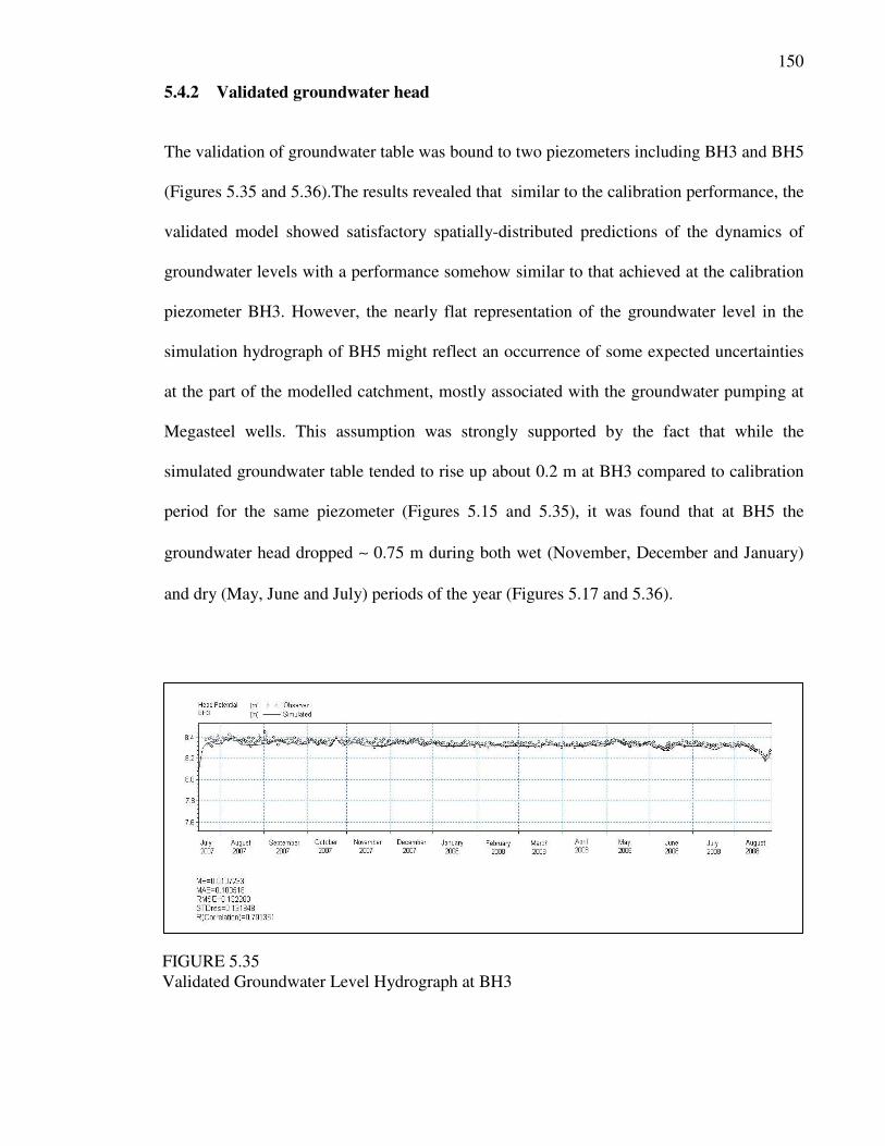
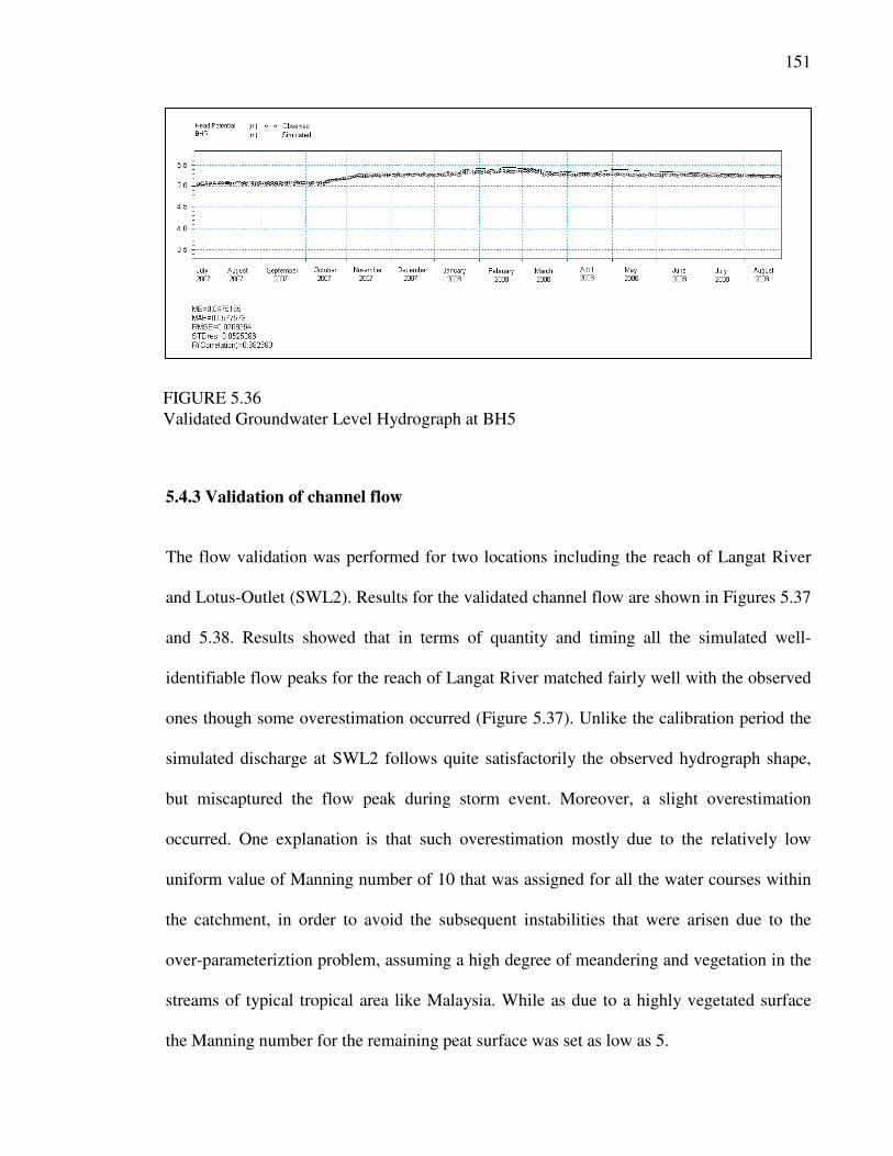
5.4.2 Validated groundwater head

The validation of groundwater table was bound to two piezometers including BH3 and BH5

(Figures 5.35 and 5.36).The results revealed that similar to the calibration performance, the

validated model showed satisfactory spatially-distributed predictions of the dynamics of

groundwater levels with a performance somehow similar to that achieved at the calibration

piezometer BH3. However, the nearly flat representation of the groundwater level in the

simulation hydrograph of BH5 might reflect an occurrence of some expected uncertainties

at the part of the modelled catchment, mostly associated with the groundwater pumping at

Megasteel wells. This assumption was strongly supported by the fact that while the

simulated groundwater table tended to rise up about 0.2 m at BH3 compared to calibration

period for the same piezometer (Figures 5.15 and 5.35), it was found that at BH5 the

groundwater head dropped ∼ 0.75 m during both wet (November, December and January)

and dry (May, June and July) periods of the year (Figures 5.17 and 5.36).

FIGURE 5.35

Validated Groundwater Level Hydrograph at BH3

151

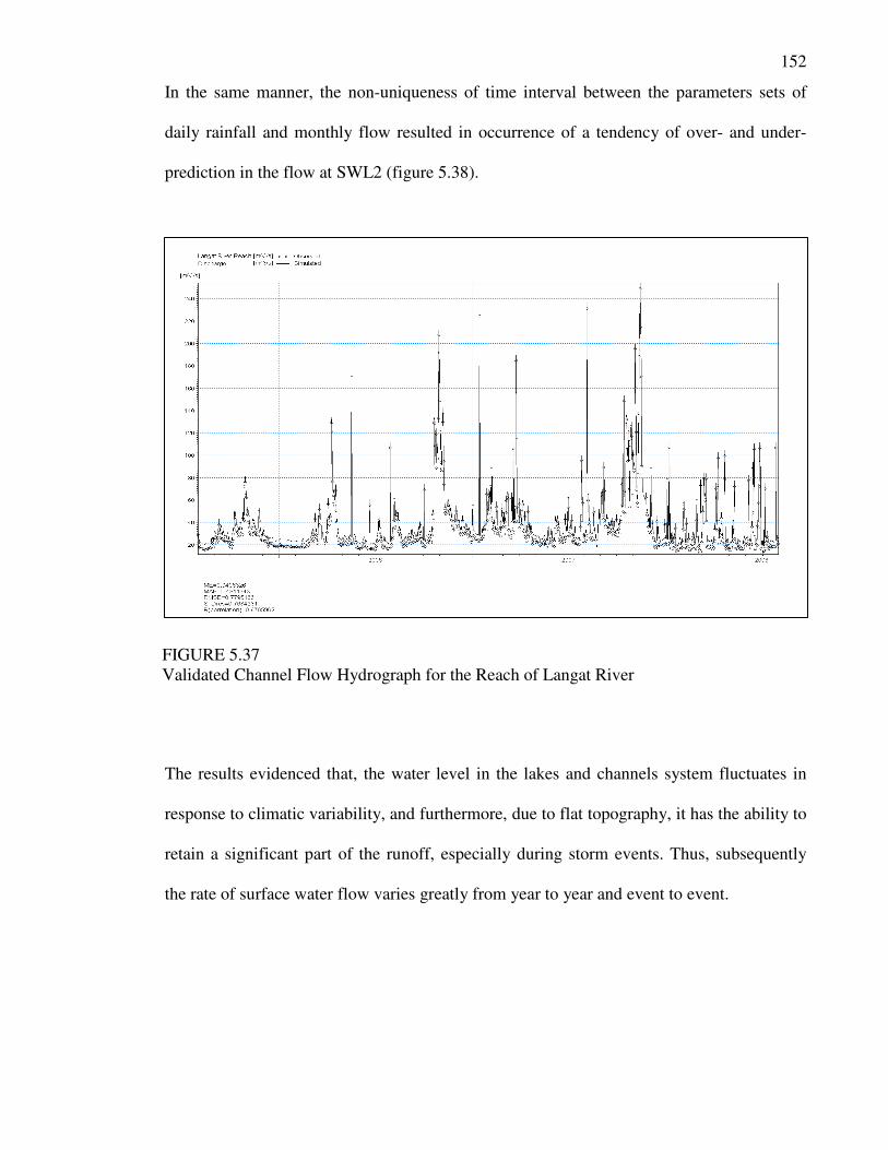
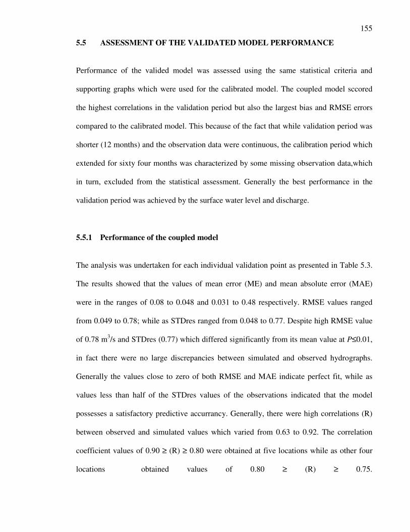
5.4.3 Validation of channel flow

The flow validation was performed for two locations including the reach of Langat River

and Lotus-Outlet (SWL2). Results for the validated channel flow are shown in Figures 5.37

and 5.38. Results showed that in terms of quantity and timing all the simulated well-

identifiable flow peaks for the reach of Langat River matched fairly well with the observed

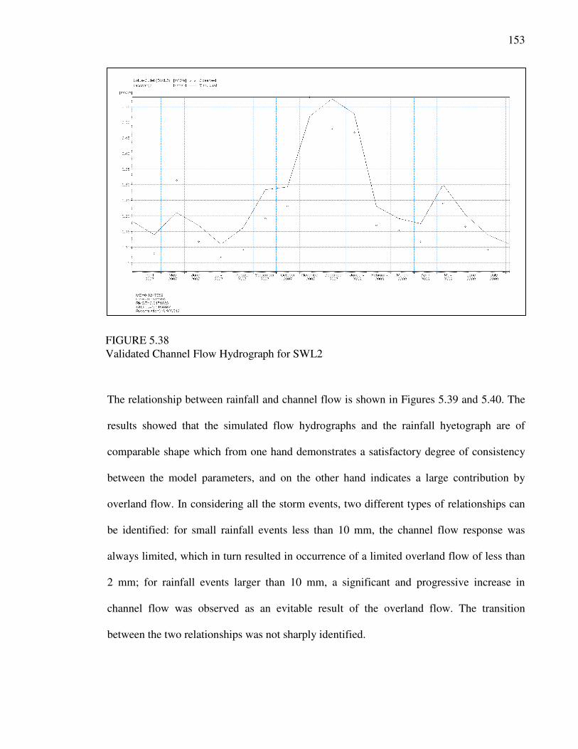
ones though some overestimation occurred (Figure 5.37). Unlike the calibration period the

simulated discharge at SWL2 follows quite satisfactorily the observed hydrograph shape,

but miscaptured the flow peak during storm event. Moreover, a slight overestimation

occurred. One explanation is that such overestimation mostly due to the relatively low

uniform value of Manning number of 10 that was assigned for all the water courses within

the catchment, in order to avoid the subsequent instabilities that were arisen due to the

over-parameteriztion problem, assuming a high degree of meandering and vegetation in the

streams of typical tropical area like Malaysia. While as due to a highly vegetated surface

the Manning number for the remaining peat surface was set as low as 5.

FIGURE 5.36

Validated Groundwater Level Hydrograph at BH5

152

In the same manner, the non-uniqueness of time interval between the parameters sets of

daily rainfall and monthly flow resulted in occurrence of a tendency of over- and under-

prediction in the flow at SWL2 (figure 5.38).

The results evidenced that, the water level in the lakes and channels system fluctuates in

response to climatic variability, and furthermore, due to flat topography, it has the ability to

retain a significant part of the runoff, especially during storm events. Thus, subsequently

the rate of surface water flow varies greatly from year to year and event to event.

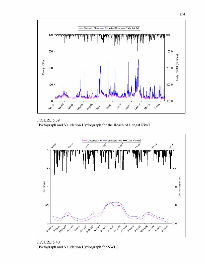
FIGURE 5.37

Validated Channel Flow Hydrograph for the Reach of Langat River

153

The relationship between rainfall and channel flow is shown in Figures 5.39 and 5.40. The

results showed that the simulated flow hydrographs and the rainfall hyetograph are of

comparable shape which from one hand demonstrates a satisfactory degree of consistency

between the model parameters, and on the other hand indicates a large contribution by

overland flow. In considering all the storm events, two different types of relationships can

be identified: for small rainfall events less than 10 mm, the channel flow response was

always limited, which in turn resulted in occurrence of a limited overland flow of less than

2 mm; for rainfall events larger than 10 mm, a significant and progressive increase in

channel flow was observed as an evitable result of the overland flow. The transition

between the two relationships was not sharply identified.

FIGURE 5.38

Validated Channel Flow Hydrograph for SWL2

154

.

FIGURE 5.40

Hyetograph and Validation Hydrograph for SWL2

FIGURE 5.39

Hyetograph and Validation Hydrograph for the Reach of Langat River

155

5.5 ASSESSMENT OF THE VALIDATED MODEL PERFORMANCE

Performance of the valided model was assessed using the same statistical criteria and

supporting graphs which were used for the calibrated model. The coupled model sccored

the highest correlations in the validation period but also the largest bias and RMSE errors

compared to the calibrated model. This because of the fact that while validation period was

shorter (12 months) and the observation data were continuous, the calibration period which

extended for sixty four months was characterized by some missing observation data,which

in turn, excluded from the statistical assessment. Generally the best performance in the

validation period was achieved by the surface water level and discharge.

5.5.1 Performance of the coupled model

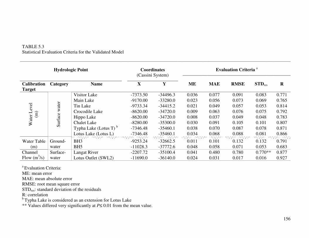
The analysis was undertaken for each individual validation point as presented in Table 5.3.

The results showed that the values of mean error (ME) and mean absolute error (MAE)

were in the ranges of 0.08 to 0.048 and 0.031 to 0.48 respectively. RMSE values ranged

from 0.049 to 0.78; while as STDres ranged from 0.048 to 0.77. Despite high RMSE value

of 0.78 m3/s and STDres (0.77) which differed significantly from its mean value at P≤0.01,

in fact there were no large discrepancies between simulated and observed hydrographs.

Generally the values close to zero of both RMSE and MAE indicate perfect fit, while as

values less than half of the STDres values of the observations indicated that the model

possesses a satisfactory predictive accurrancy. Generally, there were high correlations (R)

between observed and simulated values which varied from 0.63 to 0.92. The correlation

coefficient values of 0.90 ≥ (R) ≥ 0.80 were obtained at five locations while as other four

locations obtained values of 0.80 ≥ (R) ≥ 0.75.

156

TABLE 5.3

Statistical Evaluation Criteria for the Validated Model

a Evaluation Criteria:

ME: mean error

MAE: mean absolute error

RMSE: root mean square error

STDres: standard deviation of the residuals

R: correlation b

Typha Lake is considered as an extension for Lotus Lake

** Values differed very significantly at P≤ 0.01 from the mean value.

Hydrologic Point

Coordinates

(Cassini System)

Evaluation Criteria a

Calibration

Target

Category Name X Y ME MAE RMSE STDres R

Wat

er L

evel

(m)

Su

rfac

e w

ater

Visitor Lake -7373.50 -34496.3 0.036 0.077 0.091 0.083 0.771

Main Lake -9170.00 -33280.0 0.023 0.056 0.073 0.069 0.765

Tin Lake -9733.34 -34415.2 0.021 0.049 0.057 0.053 0.814

Crocodile Lake -8620.00 -34720.0 0.009 0.063 0.076 0.075 0.792

Hippo Lake -8620.00 -34720.0 0.008 0.037 0.049 0.048 0.783

Chalet Lake -8280.00 -35300.0 0.030 0.091 0.105 0.101 0.807

Typha Lake (Lotus T) b

-7346.48 -35460.1 0.038 0.070 0.087 0.078 0.871

Lotus Lake (Lotus L) -7346.48 -35460.1 0.034 0.068 0.088 0.081 0.866

Water Table

(m)

Ground-

water

BH3 -9253.24 -32662.5 0.011 0.101 0.132 0.132 0.791

BH5 -11028.3 -37772.6 0.048 0.058 0.071 0.053 0.683

Channel

Flow (m3/s)

Surface-

water

Langat River -2207.72 -35100.4 0.041 0.480 0.780 0.770** 0.877

Lotus Outlet (SWL2) -11690.0 -36140.0 0.024 0.031 0.017 0.016 0.927

156

157

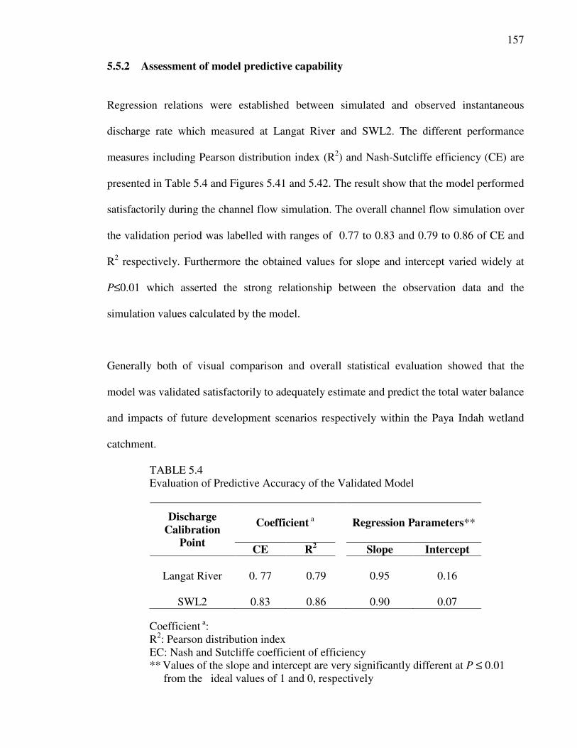
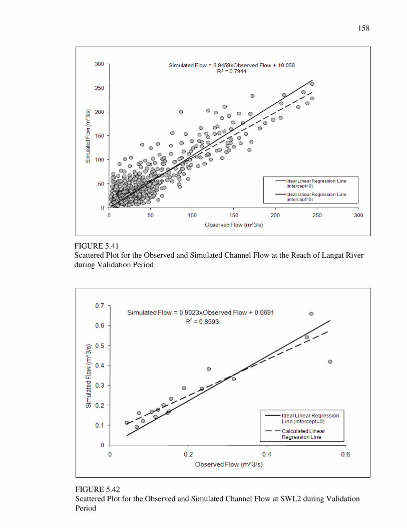
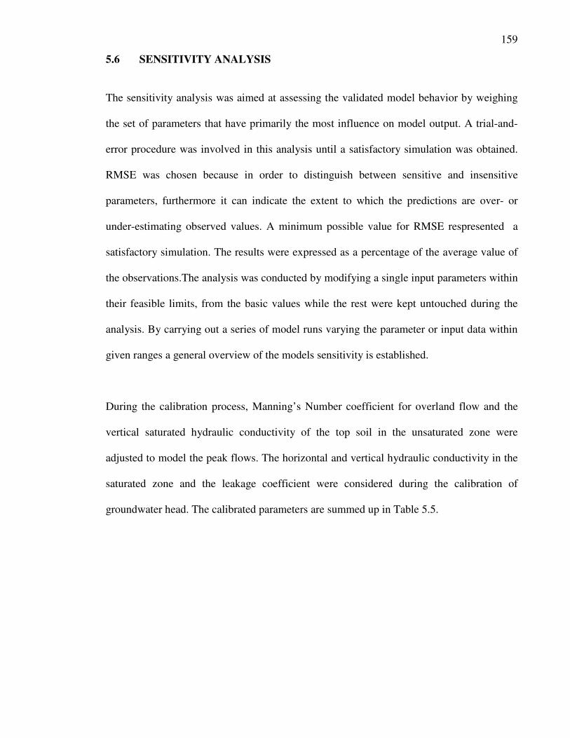
5.5.2 Assessment of model predictive capability

Regression relations were established between simulated and observed instantaneous

discharge rate which measured at Langat River and SWL2. The different performance

measures including Pearson distribution index (R2) and Nash-Sutcliffe efficiency (CE) are

presented in Table 5.4 and Figures 5.41 and 5.42. The result show that the model performed

satisfactorily during the channel flow simulation. The overall channel flow simulation over

the validation period was labelled with ranges of 0.77 to 0.83 and 0.79 to 0.86 of CE and

R2 respectively. Furthermore the obtained values for slope and intercept varied widely at

P≤0.01 which asserted the strong relationship between the observation data and the

simulation values calculated by the model.

Generally both of visual comparison and overall statistical evaluation showed that the

model was validated satisfactorily to adequately estimate and predict the total water balance

and impacts of future development scenarios respectively within the Paya Indah wetland

catchment.

TABLE 5.4

Evaluation of Predictive Accuracy of the Validated Model

Discharge

Calibration

Point

Coefficient a

Regression Parameters**

CE R2 Slope Intercept

Langat River 0. 77 0.79 0.95 0.16

SWL2

0.83

0.86

0.90

0.07

Coefficient a:

R2: Pearson distribution index

EC: Nash and Sutcliffe coefficient of efficiency

** Values of the slope and intercept are very significantly different at P ≤ 0.01

from the ideal values of 1 and 0, respectively

158

FIGURE 5.41

Scattered Plot for the Observed and Simulated Channel Flow at the Reach of Langat River

during Validation Period

FIGURE 5.42

Scattered Plot for the Observed and Simulated Channel Flow at SWL2 during Validation

Period

159

5.6 SENSITIVITY ANALYSIS

The sensitivity analysis was aimed at assessing the validated model behavior by weighing

the set of parameters that have primarily the most influence on model output. A trial-and-

error procedure was involved in this analysis until a satisfactory simulation was obtained.

RMSE was chosen because in order to distinguish between sensitive and insensitive

parameters, furthermore it can indicate the extent to which the predictions are over- or

under-estimating observed values. A minimum possible value for RMSE respresented a

satisfactory simulation. The results were expressed as a percentage of the average value of

the observations.The analysis was conducted by modifying a single input parameters within

their feasible limits, from the basic values while the rest were kept untouched during the

analysis. By carrying out a series of model runs varying the parameter or input data within

given ranges a general overview of the models sensitivity is established.

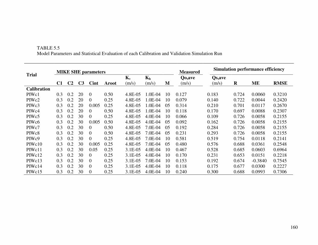
During the calibration process, Manning’s Number coefficient for overland flow and the

vertical saturated hydraulic conductivity of the top soil in the unsaturated zone were

adjusted to model the peak flows. The horizontal and vertical hydraulic conductivity in the

saturated zone and the leakage coefficient were considered during the calibration of

groundwater head. The calibrated parameters are summed up in Table 5.5.

160

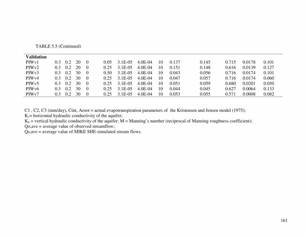
TABLE 5.5

Model Parameters and Statistical Evaluation of each Calibration and Validation Simulation Run

Trial

MIKE SHE parameters Measured Simulation performance efficiency

C1 C2 C3 Cint Aroot

Kv

(m/s) Kh

(m/s) M

Qo,ave

(m/s)

Qs,ave

(m/s) R ME RMSE

Calibration

PIWc1 0.3 0.2 20 0 0.50 4.8E-05 1.0E-04 10 0.127 0.183 0.724 0.0060 0.3210

PIWc2 0.3 0.2 20 0 0.25 4.8E-05 1.0E-04 10 0.079 0.140 0.722 0.0044 0.2420

PIWc3 0.3 0.2 20 0.005 0.25 4.8E-05 1.0E-04 05 0.314 0.210 0.701 0.0117 0.2670

PIWc4 0.3 0.2 20 0 0.50 4.8E-05 1.0E-04 10 0.118 0.170 0.697 0.0088 0.2307

PIWc5 0.3 0.2 30 0 0.25 4.8E-05 4.0E-04 10 0.066 0.109 0.726 0.0058 0.2155

PIWc6 0.3 0.2 30 0.005 0.50 4.8E-05 4.0E-04 05 0.092 0.162 0.726 0.0058 0.2155

PIWc7 0.3 0.2 30 0 0.50 4.8E-05 7.0E-04 05 0.192 0.284 0.726 0.0058 0.2155

PIWc8 0.3 0.2 30 0 0.50 4.8E-05 7.0E-04 05 0.231 0.293 0.726 0.0058 0.2155

PIWc9 0.3 0.2 30 0 0.25 4.8E-05 7.0E-04 10 0.581 0.519 0.754 0.0118 0.2141

PIWc10 0.3 0.2 30 0.005 0.25 4.8E-05 7.0E-04 05 0.480 0.576 0.688 0.0361 0.2548

PIWc11 0.3 0.2 30 0.05 0.25 3.1E-05 4.0E-04 10 0.467 0.528 0.685 0.0603 0.6964

PIWc12 0.3 0.2 30 0 0.25 3.1E-05 4.0E-04 10 0.170 0.231 0.653 0.0151 0.2218

PIWc13 0.3 0.2 30 0 0.25 3.1E-05 7.0E-04 10 0.153 0.192 0.674 -0.3840 0.7545

PIWc14 0.3 0.2 30 0 0.25 3.1E-05 4.0E-04 10 0.118 0.175 0.677 0.0300 0.2227

PIWc15 0.3 0.2 30 0 0.25 3.1E-05 4.0E-04 10 0.240 0.300 0.688 0.0993 0.7306

160

161

TABLE 5.5 (Continued)

C1 , C2, C3 (mm/day), Cint, Aroot = actual evapotranspiration parameters of the Kristensen and Jensen model (1975);

Kv= horizontal hydraulic conductivity of the aquifer;

Kh = vertical hydraulic conductivity of the aquifer; M = Manning’s number (reciprocal of Manning roughness coefficient);

Qo,ave = average value of observed streamflow;

Qs,ave = average value of MIKE SHE-simulated stream flows.

Validation

PIWv1 0.3 0.2 20 0 0.05 3.1E-05 4.0E-04 10 0.137 0.145 0.715 0.0178 0.101

PIWv2 0.3 0.2 20 0 0.25 3.1E-05 4.0E-04 10 0.151 0.148 0.616 0.0139 0.127

PIWv3 0.3 0.2 30 0 0.50 3.1E-05 4.0E-04 10 0.043 0.056 0.716 0.0174 0.101

PIWv4 0.3 0.2 30 0 0.25 3.1E-05 4.0E-04 10 0.047 0.057 0.716 0.0174 0.060

PIWv5 0.3 0.2 30 0 0.25 3.1E-05 4.0E-04 10 0.051 0.059 0.680 0.0201 0.050

PIWv6 0.3 0.2 30 0 0.25 3.1E-05 4.0E-04 10 0.044 0.045 0.627 0.0064 0.133

PIWv7 0.3 0.2 30 0 0.25 3.1E-05 4.0E-04 10 0.053 0.055 0.571 0.0008 0.082

161

162

One of the main required implementations from the Paya Indah wetland model is

estimation of the water balance for the modelled catchment and the stress on the water

resource caused by adjacent development of Cyberjaya and groundwater abstraction at

Megasteel Company’s property. Looking at the overall water balance components it is clear

that evapotranspiration accounts for the largest water loss from the model area, bearing in

mind the tropical climate conditions of the area. It was thus essential to test the sensitivity

of the actual evapotranspiration. The sensitivity runs were performed on different input

variables mainly potential evapotranspiration, inflow depletion at SWL1, and groundwater

abstraction. The latter was discussed comprehensively in Chapter 7.3 of this thesis. The test

also included some other inputs parameter such as hydraulic conductivity and storage

coefficient however, they were found of insignificant sensitivity thus excluded from the

discussion. Generally, the calibrated model values and statistics represented the control run

for all the sensitivity runs.

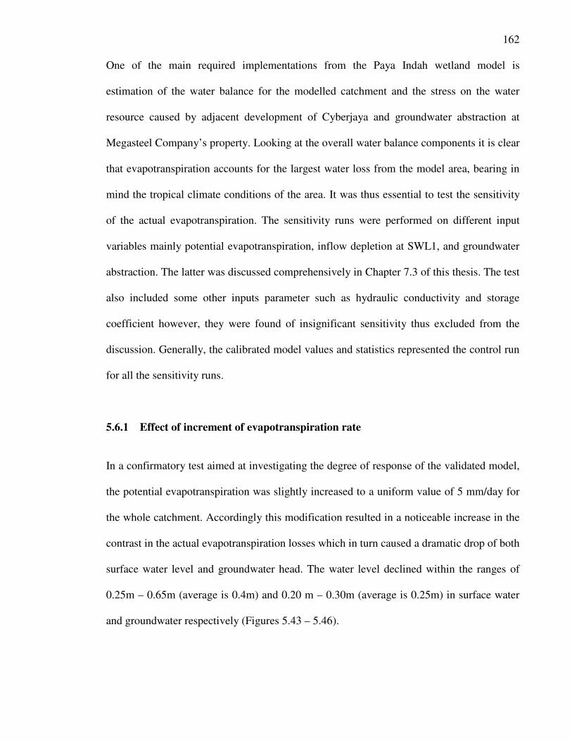
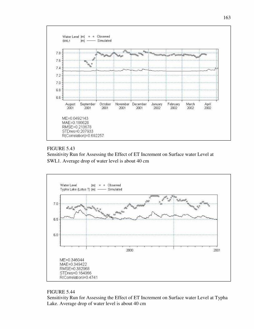
5.6.1 Effect of increment of evapotranspiration rate

In a confirmatory test aimed at investigating the degree of response of the validated model,

the potential evapotranspiration was slightly increased to a uniform value of 5 mm/day for

the whole catchment. Accordingly this modification resulted in a noticeable increase in the

contrast in the actual evapotranspiration losses which in turn caused a dramatic drop of both

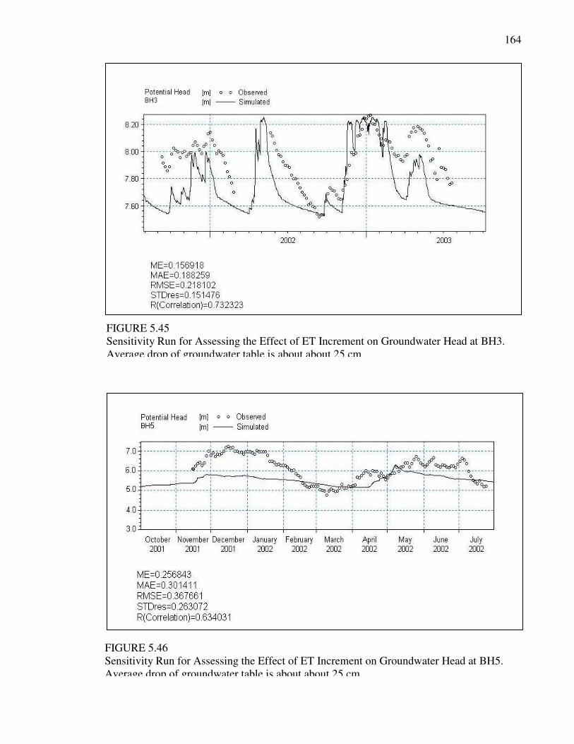
surface water level and groundwater head. The water level declined within the ranges of

0.25m – 0.65m (average is 0.4m) and 0.20 m – 0.30m (average is 0.25m) in surface water

and groundwater respectively (Figures 5.43 – 5.46).

163

FIGURE 5.43

Sensitivity Run for Assessing the Effect of ET Increment on Surface water Level at

SWL1. Average drop of water level is about 40 cm

FIGURE 5.44

Sensitivity Run for Assessing the Effect of ET Increment on Surface water Level at Typha

Lake. Average drop of water level is about 40 cm

164

FIGURE 5.46

Sensitivity Run for Assessing the Effect of ET Increment on Groundwater Head at BH5.

Average drop of groundwater table is about about 25 cm

FIGURE 5.45

Sensitivity Run for Assessing the Effect of ET Increment on Groundwater Head at BH3.

Average drop of groundwater table is about about 25 cm

165

The model demonstrated that increment and uniform distribution of the potential

evapotranspiration had a greater effect on the surface water level and, surprisingly, the

groundwater head as well. This phenomenon was observed at the Kuala Langat peat swamp

forest upstream of the modelled catchment where the water table normally is close to or

rises above the surface depending on the season (i.e. wet and dry). However, it seemed that

this modification of evapotranspiration input did not affect the capability of the model to

adequately simulate the dynamics in both surface water and groundwater. In fact it was

found that assigning the reference evapotranspiration rate in a form of an actual daily

timeseries that distributed evenly over the year; improve the model performance much

better than the uniform value of 4 mm/day does. This finding efficienctly improved the

simulation accuracy in both calibration or validation periods.

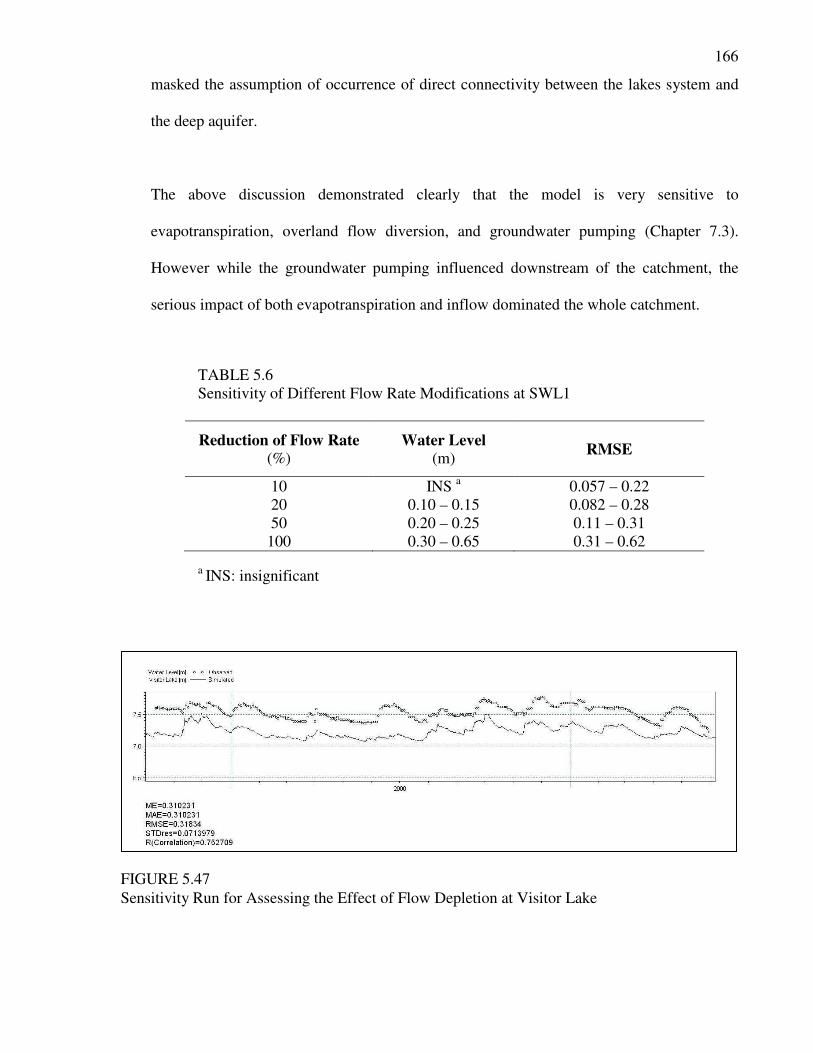
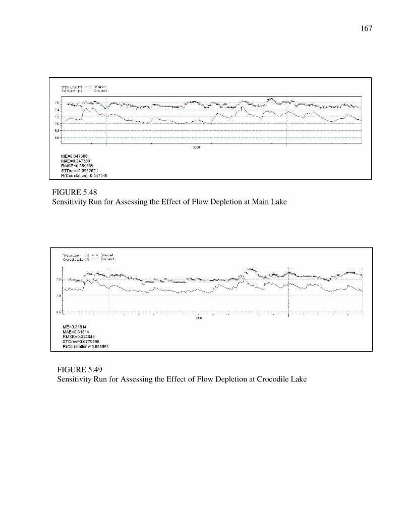
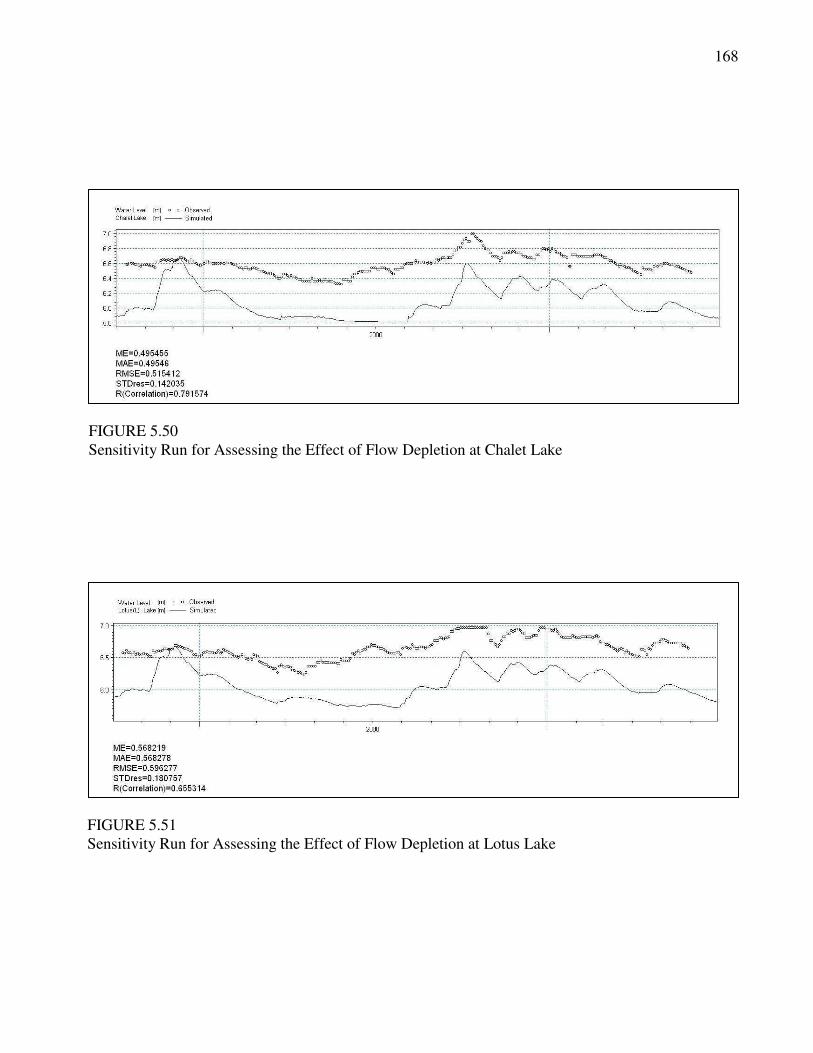
5.6.2 Effect of depletion of the inflow

The sensitivity runs were performed to examine the change of the model upon depletion of

inflow at SWL1. No significant difference was observed due to reduction of the flow rate

by 10% however by 20 % and 50 % it dropped 0.10 to 0.15 m and 0.20 m to 0.25 m

respectively (Table 5.6). While as 100 % depletion of the incoming flow to the system

caused a drop within a range of 0.3 m to 0.60 m (Figures 5.47 – 5.52). However the water

level at Driftwood, Tin, Perch and Marsh Lakes did not response to these modifications.

Despite the seepage from overland flow, the fact that outer boundary of the Tin Lake

extends some 2.5 km adjacent to the Kuala Langat swamp forest indicates of inflow from

the shallow peat aquifer. This observation explained the tendency of these lakes to act as a

sub-catchment within the Paya Indah Lakes system. In contrast the deep aquifer

groundwater head showed insignificant response to the flow modifications. This result

166

masked the assumption of occurrence of direct connectivity between the lakes system and

the deep aquifer.

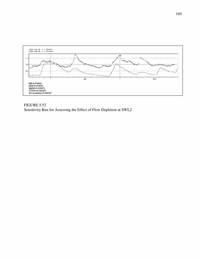
The above discussion demonstrated clearly that the model is very sensitive to

evapotranspiration, overland flow diversion, and groundwater pumping (Chapter 7.3).

However while the groundwater pumping influenced downstream of the catchment, the

serious impact of both evapotranspiration and inflow dominated the whole catchment.

TABLE 5.6

Sensitivity of Different Flow Rate Modifications at SWL1

Reduction of Flow Rate

(%) Water Level

(m)

RMSE

10 INS a

0.057 – 0.22

20 0.10 – 0.15 0.082 – 0.28

50 0.20 – 0.25 0.11 – 0.31

100 0.30 – 0.65 0.31 – 0.62

a INS: insignificant

FIGURE 5.47

Sensitivity Run for Assessing the Effect of Flow Depletion at Visitor Lake

167

FIGURE 5.48

Sensitivity Run for Assessing the Effect of Flow Depletion at Main Lake

FIGURE 5.49

Sensitivity Run for Assessing the Effect of Flow Depletion at Crocodile Lake

168

FIGURE 5.51

Sensitivity Run for Assessing the Effect of Flow Depletion at Lotus Lake

FIGURE 5.50

Sensitivity Run for Assessing the Effect of Flow Depletion at Chalet Lake

169

FIGURE 5.52

Sensitivity Run for Assessing the Effect of Flow Depletion at SWL2

CHAPTER V MODEL CALIBRATION AND VALIDATION

Documents

Transcript of CHAPTER V MODEL CALIBRATION AND VALIDATION