Chapter Six

Normal Curves and Sampling Probability

Distributions

SECTION 5SECTION 5

The Central Limit The Central Limit TheoremTheorem

The Central Limit Theorem is The Central Limit Theorem is applied in the following ways:applied in the following ways:

A given population has fixed parameters µ and σ .For each population, there are very many samples of size n, which can be taken. Each of these samples has a sample mean x. The x statistic varies from sample to sample. The Central Limit Theorem tells us what to expect about the sample means.

If x is normally distributed for any size sample, or if the sample

size is 30 or more, the sample means will be normally

distributed.

When working with any normal distribution, we have to

know the mean of the distribution and the standard

deviation. The Central Limit Theorem relates the mean

and the standard deviation of the original x to the mean

and standard deviation of x .

When working with normal distribution probabilities, we

must convert all values to z-scores.

The Central Limit Theorem is used to investigate the probability

of a sample mean being in a given interval.

Since we will be working with normal

distributions, the x values in the given

interval must be converted to z-scores.

There are three formulas, all which are

equivalent, which may be used to

convert from an x value to a z-score.

The simplest formula is

The deviation of x value from the mean is divided by the

standard deviation of the distribution σ x. To use this

version, first we calculate σ xby dividing σ by n. Then substitute.

You may prefer to directly substitute the fraction σn for

σ x in the denominator and use either of the two formulas that follow. You could use ...

z =x−μσ x

or invert and multiply to get the formulayou are to use in this class:

z =x−μσn

z =x−μ( ) n

σ

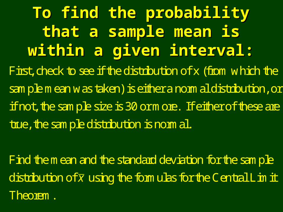
To find the probability that a sample To find the probability that a sample mean is within a given interval:mean is within a given interval:

First, check to see if the distribution of x (from which the

sample mean was taken) is either a normal distribution, or

if not, the sample size is 30 or more. If either of these are

true, the sample distribution is normal.

Find the mean and the standard deviation for the sample

distribution of x using the formulas for the Central Limit

Theorem.

Convert each endpoint of the given interval to the standard

normal z-score.

Rewrite the problem with the z-score interval.

Sketch a standard normal distribution curve and shade the

area you wish to calculate.

Use the table for standard normal probability distribution

to calculate the area, and thus, the probability.

Case 1Case 1When a variable x has a mean of μx, and a standard deviation of σ x, and is normally distributed. For a random sample of any size n, the following statements about the sampling distribution of x are true.

1. The distribution of x is normal.

2. The mean of the sample means is equal to the

mean of the population. That is: μx =μ

3. The standard deviation of the distributions of the sample means is called the standard error of the mean and is smaller than the

distribution of x by a factor of 1n.

That is: σ x =σn.

CASE 2CASE 2When a variable x comes from any

type of distribution, no matter how

unusual, as long as the random sample

has at least 30 members, then the

following statements about the

distribution of the sample size are true.

1. The distribution of x is normal.

2. The mean of the sample means is equal to the

mean of the population. That is: μx =μ

3. The standard deviation of the distributions of the sample means is called the standard error of the mean and is smaller than the

distribution of x by a factor of 1n.

That is: σ x =σn.

Sampling DistributionSampling Distribution

A probability distribution

for the sample statistic

we are using.

Example of a Sampling Example of a Sampling DistributionDistribution

Select samples with two elements

each (in sequence with

replacement) from the set

{1, 2, 3, 4, 5, 6}.

Constructing a Sampling Distribution Constructing a Sampling Distribution of the Mean for Samples of Size n = 2of the Mean for Samples of Size n = 2

List all samples and compute the mean of each sample.sample: mean: sample: mean{1,1} 1.0 {1,6} 3.5{1,2} 1.5 {2,1} 1.5{1,3} 2.0 {2,2} 2.0{1,4} 2.5 … ...{1,5} 3.0

How many different samples are there?How many different samples are there? 3636

Sampling Distribution of the MeanSampling Distribution of the Mean

p1.0 1/361.5 2/362.0 3/362.5 4/363.0 5/363.5 6/364.0 5/364.5 4/365.0 3/365.5 2/36 6.0 1/36

x

Sampling Distribution Sampling Distribution HistogramHistogram

Let x be a random variable with a

normal distribution with mean μ and standard deviation σ . Let x be the sample mean corresponding to random samples of size n taken from the distribution.

The following are true:The following are true:

1. The x distribution is a normal distribution.

2. The mean of the x distribution is μ (the same mean as the original distribution).

3. The standard deviation of the x distribution

is σn (the standard deviation of the original

distribution, divided by the square root of the sample size).

We can use this theorem to draw conclusions about means of samples taken from normal distributions.

If the original distribution is normal, then the sampling distribution will be normal.

The Mean of the Sampling The Mean of the Sampling DistributionDistribution

μx

The mean of the sampling distribution is equal to the mean of the original distribution.

μx = μ

The Standard Deviation of the The Standard Deviation of the Sampling DistributionSampling Distribution

σ x

The standard deviation of the sampling distribution is equal to the standard deviation of the original distribution divided by the square

root of the sample size.

σ x =σ

n

The Central

Limit Theorem

As the sample size continue to

increase closer and closer

to the population size the

following statements are true.

1. The sample will have

a normal distribution.

2. The sample mean will

approach the population

mean. limn→ N

x=μ( )

3. The standard deviation will take on the

intermediate value of the population

standard deviation divided by the

square root of the sample size. However,

because of the increasing sample size

this value will approach zero.

limn→ N

σ x =limn→ N

σn=0⎛

⎝⎜⎞⎠⎟

4. The probability of an interval that

contains the population mean

will approach 1.

limn→ N

P x1 < μ < x2( ) =1( )

5. The probability of an interval

that does NOT contain the

population mean will approach 0.

limn→ N

P x1 < μ( ) =0( )

or

limn→ N

P x> μ( ) =0( )

***Note***

As the sample size increases to the population size

Graph 1 → Graph 2→ Graph 3the graphs get closer and closer to the population mean.

The Central Limit Theorem states that

if the probability interval contains the

population mean and the sample size

continues to increase closer and closer

to the population size then the probability

will continue to increase and get closer

and closer to 1.

or

The Central Limit Theorem states that

if the probability interval does not

contain the population mean and the

sample size continues increase closer

and closer to the population size then

the probability will continue to decrease

and get closer and closer to 0.

Sample

Questions

1.1.

Suppose that it is known that the time

spent by customers in the local coffee

shop is normally distributed with a

mean of 24 minutes and a standard

deviation of 6 minutes.

a.Find the probability that an individual

customer will spend more than 26

minutes in the coffee shop.

P x > 26( )

P z>26−24

6⎛⎝⎜

⎞⎠⎟

P z>26

⎛⎝⎜

⎞⎠⎟

P z> 0.33( )0.5000−0.1293

0.3707

0.33

b.Find the probability that a random sample

of 9 customers will have a mean stay of

more than 26 minutes in the coffee shop. P x > 26( )

P z>26−24( ) 9

6

⎛

⎝⎜⎞

⎠⎟

P z>2 3( )6

⎛⎝⎜

⎞⎠⎟

P z>66

⎛⎝⎜

⎞⎠⎟

P z>1.00( )0.5000−0.3413

0.1587

1.00

c.Find the probability that a random sample

of 64 customers will have a mean stay of

more than 26 minutes in the coffee shop. P x > 26( )

P z>26−24( ) 64

6

⎛

⎝⎜⎞

⎠⎟

P z>2 8( )6

⎛⎝⎜

⎞⎠⎟

P z>166

⎛⎝⎜

⎞⎠⎟

P z> 2.67( )0.5000−0.4962

0.0038

2.67

d.Find the probability that a random sample

of 100 customers will have a mean stay of

more than 26 minutes in the coffee shop. P x > 26( )

P z>26−24( ) 100

6

⎛

⎝⎜⎞

⎠⎟

P z>2 10( )6

⎛⎝⎜

⎞⎠⎟

P z>206

⎛⎝⎜

⎞⎠⎟

P z> 3.33( )0.5000−0.4996

0.0004

3.33

e.Find the probability that a random sample

of 144 customers will have a mean stay of

more than 26 minutes in the coffee shop. P x > 26( )

P z>26−24( ) 144

6

⎛

⎝⎜⎞

⎠⎟

P z>2 12( )6

⎛⎝⎜

⎞⎠⎟

P z>246

⎛⎝⎜

⎞⎠⎟

P z> 4.00( )0.5000−0.4999

0.0001

4.00

e. The Central Limit Theorem states that

if the probability interval does not

contain the population mean and the

sample size continues increase closer

and closer to the population size then

the probability will continue to decrease

and get closer and closer to 0.

2.2.

Suppose that it is known that the time

spent by customers in the local coffee

shop is normally distributed with a

mean of 24 minutes and a standard

deviation of 6 minutes.

a.Find the probability that an individual

customer will spend between 22 to 25

minutes in the coffee shop.P 22 ≤x≤25( )

P22−24

6≤z≤

25−246

⎛⎝⎜

⎞⎠⎟

P−26

≤z≤16

⎛⎝⎜

⎞⎠⎟

P −0.33≤z≤0.17( )0.1293+0.0675

0.1968

-0.33 0.17

b.

Find the probability that a random sample

of 9 customers will have a mean stay in

the coffee shop between 22 to 25 minutes.

P 22 ≤x≤25( )

P22−24 9( )

6≤z≤

25−24( ) 96

⎛

⎝⎜⎜

⎞

⎠⎟⎟

P−2( ) 3( )6

≤z≤1( ) 3( )6

⎛⎝⎜

⎞⎠⎟

P−66

≤z≤36

⎛⎝⎜

⎞⎠⎟

P −1.00 ≤z≤0.50( )0.3413+ 0.1915

0.5328

-1.00 0.50

c.

Find the probability that a random sample

of 64 customers will have a mean stay in

the coffee shop between 22 to 25 minutes.

P 22 ≤x≤25( )

P22−24 64( )

6≤z≤

25−24( ) 646

⎛

⎝⎜⎜

⎞

⎠⎟⎟

P−2( ) 8( )6

≤z≤1( ) 8( )6

⎛⎝⎜

⎞⎠⎟

P−166

≤z≤86

⎛⎝⎜

⎞⎠⎟

P −2.67 ≤z≤1.33( )0.4962 + 0.4082

0.9044

-2.67 1.33

d.

Find the probability that a random sample

of 100 customers will have a mean stay in

the coffee shop between 22 to 25 minutes.

P 22 ≤x≤25( )

P22−24 100( )

6≤z≤

25−24( ) 1006

⎛

⎝⎜⎜

⎞

⎠⎟⎟

P−2( ) 10( )

6≤z≤

1( ) 10( )6

⎛⎝⎜

⎞⎠⎟

P−206

≤z≤106

⎛⎝⎜

⎞⎠⎟

P −3.33≤z≤1.67( )0.4996 +0.4525

0.9521

-3.33 1.67

e.

Find the probability that a random sample

of 144 customers will have a mean stay in

the coffee shop between 22 to 25 minutes.

P 22 ≤x≤25( )

P22−24 144( )

6≤z≤

25−24( ) 1446

⎛

⎝⎜⎜

⎞

⎠⎟⎟

P−2( ) 12( )

6≤z≤

1( ) 12( )6

⎛⎝⎜

⎞⎠⎟

P−246

≤z≤126

⎛⎝⎜

⎞⎠⎟

P −4.00 ≤z≤2.00( )0.4999 + 0.4772

0.9771

-4.00 2.00

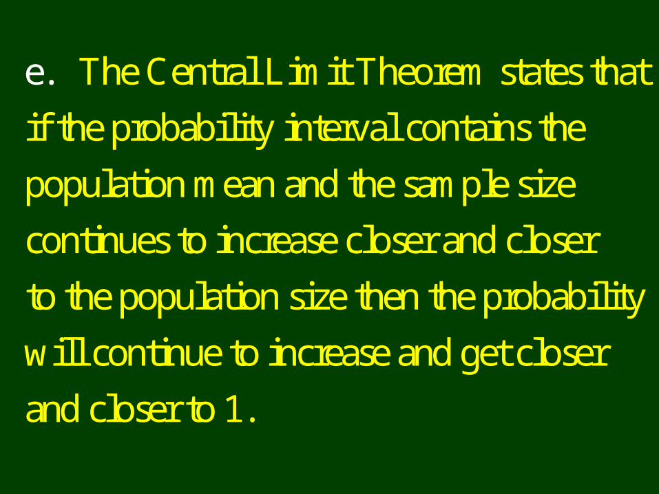
e. The Central Limit Theorem states that

if the probability interval contains the

population mean and the sample size

continues to increase closer and closer

to the population size then the probability

will continue to increase and get closer

and closer to 1.

THE END