Chapter Matrix Two Person Games
140
Game Theory, Ch1.2 1 Game Theory Chapter 1 Matrix Two‐Person Games Instructor: Chih‐Wen Chang Wenson Chang @ NCKU
Transcript of Chapter Matrix Two Person Games
Game Theory, Ch1.2 1
Game Theory
Chapter 1Matrix Two‐Person Games
Instructor: Chih‐Wen Chang
Wenson Chang @ NCKU
Contents
• 1.1 The basic
• 1.2 The von Neumann minimax theorem
• 1.3 Mixed strategies
• 1.4 Solving 2 × 2 games graphically
• 1.5 Graphical solution of 2 ×m and n × 2 games
• 1.6 Best response strategies
Wenson Chang @ NCKU Game Theory, Ch1.2 2
The Basic
• A game involves a number of players N, a set of strategies for each player, and a payoff that quantitatively describes the outcome of each play of the game in terms of the amount that each player wins or loses.
• A strategy for each player can be very complicated because it is a plan, determined at the start of the game, that describes what a player will do in every possible situation.
Wenson Chang @ NCKU Game Theory, Ch1.2 3
A Two‐Person Zero Sum Game
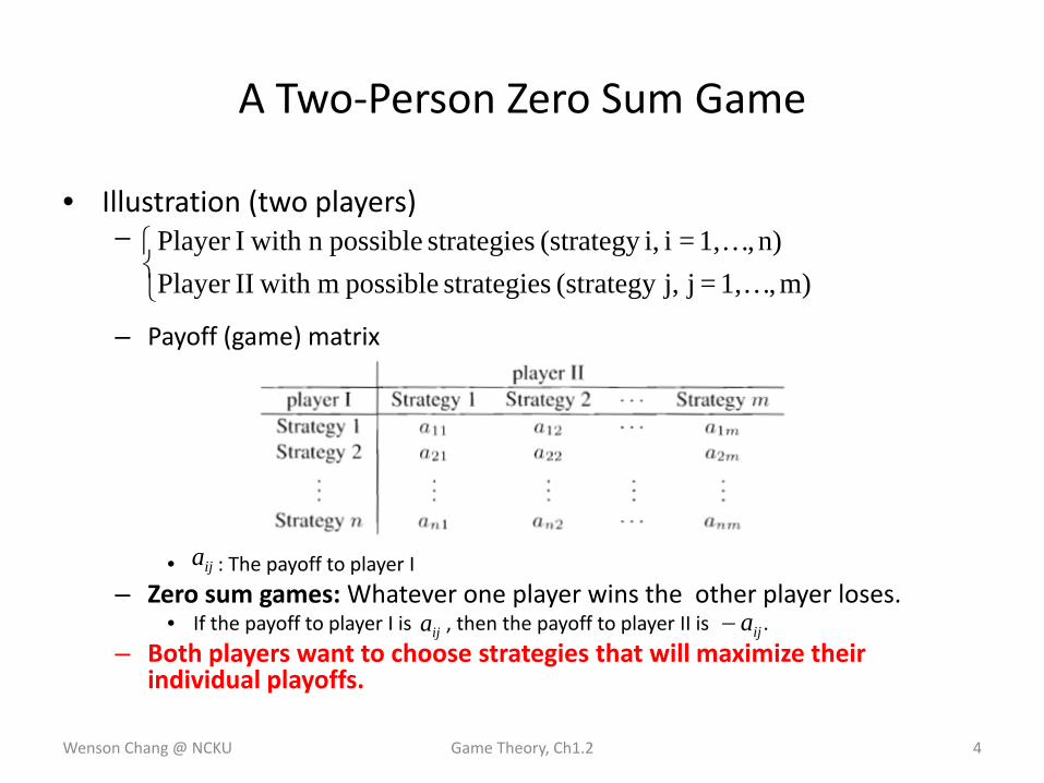
• Illustration (two players)–
– Payoff (game) matrix
• : The payoff to player I
– Zero sum games:Whatever one player wins the other player loses.• If the payoff to player I is , then the payoff to player II is .
– Both players want to choose strategies that will maximize their individual playoffs.
Wenson Chang @ NCKU Game Theory, Ch1.2 4
⎩⎨⎧
m),…1,=j j,(strategy strategies possible m with IIPlayer n),…1,=i i,(strategy strategies possiblen with IPlayer
ija
ija ija−
Constant Sum Games
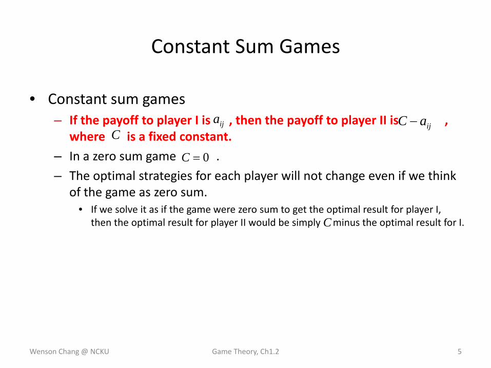
• Constant sum games– If the payoff to player I is , then the payoff to player II is ,
where is a fixed constant.
– In a zero sum game .
– The optimal strategies for each player will not change even if we think of the game as zero sum.
• If we solve it as if the game were zero sum to get the optimal result for player I, then the optimal result for player II would be simply minus the optimal result for I.
Wenson Chang @ NCKU Game Theory, Ch1.2 5
ijaijaC −
C
0=C
C
Example 1.1
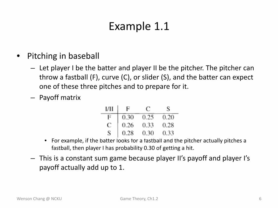
• Pitching in baseball– Let player I be the batter and player II be the pitcher. The pitcher can
throw a fastball (F), curve (C), or slider (S), and the batter can expect one of these three pitches and to prepare for it.
– Payoff matrix
• For example, if the batter looks for a fastball and the pitcher actually pitches a fastball, then player I has probability 0.30 of getting a hit.
– This is a constant sum game because player II’s payoff and player I’s payoff actually add up to 1.
Wenson Chang @ NCKU Game Theory, Ch1.2 6
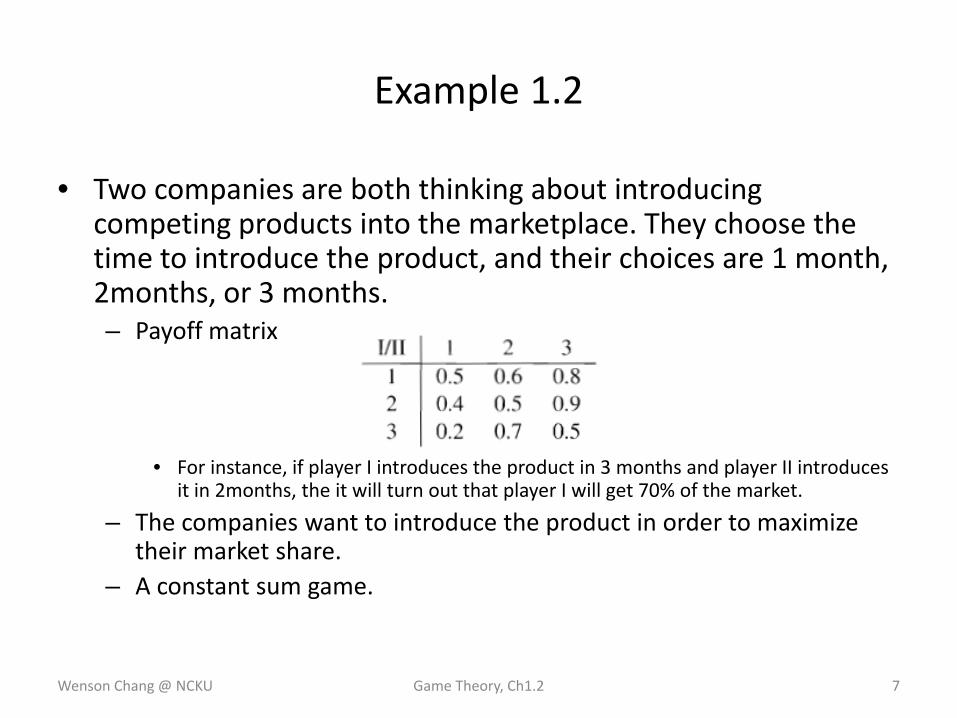
• Two companies are both thinking about introducing competing products into the marketplace. They choose the time to introduce the product, and their choices are 1 month, 2months, or 3 months.– Payoff matrix
• For instance, if player I introduces the product in 3 months and player II introduces it in 2months, the it will turn out that player I will get 70% of the market.
– The companies want to introduce the product in order to maximize their market share.
– A constant sum game.
Wenson Chang @ NCKU Game Theory, Ch1.2 7
Example 1.2
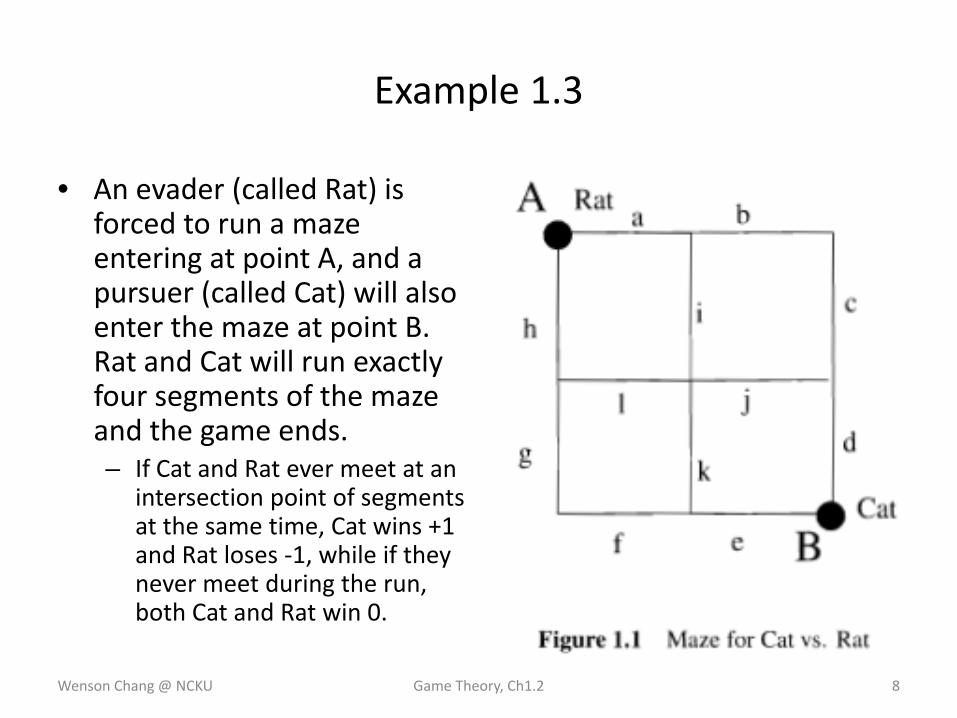
• An evader (called Rat) is forced to run a maze entering at point A, and a pursuer (called Cat) will also enter the maze at point B. Rat and Cat will run exactly four segments of the maze and the game ends.– If Cat and Rat ever meet at an
intersection point of segments at the same time, Cat wins +1 and Rat loses ‐1, while if they never meet during the run, both Cat and Rat win 0.
Wenson Chang @ NCKU Game Theory, Ch1.2 8
Example 1.3
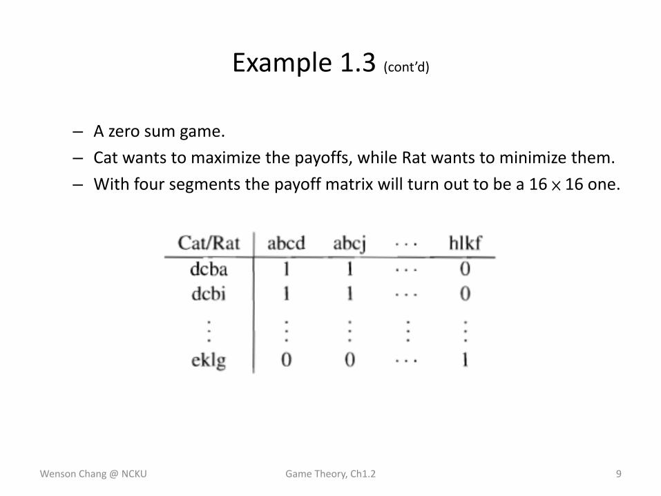
– A zero sum game.
– Cat wants to maximize the payoffs, while Rat wants to minimize them.
– With four segments the payoff matrix will turn out to be a 16 × 16 one.
Wenson Chang @ NCKU Game Theory, Ch1.2 9
Example 1.3 (cont’d)
• 2 × 2 Nim.– Four pennies are set out in two piles of two pennies each.
– Player I chooses a pile and then decides to remove one or two pennies from the pile chosen.
– Then player II chooses a pile with at least one penny and decides how many pennies to remove.
– Then player I starts the second round with the same rules.
– When both piles have no pennies, the game ends and the loser is the player who removed the last penny.
– The loser pays the winner one dollar.
Wenson Chang @ NCKU Game Theory, Ch1.2 10
Example 1.4
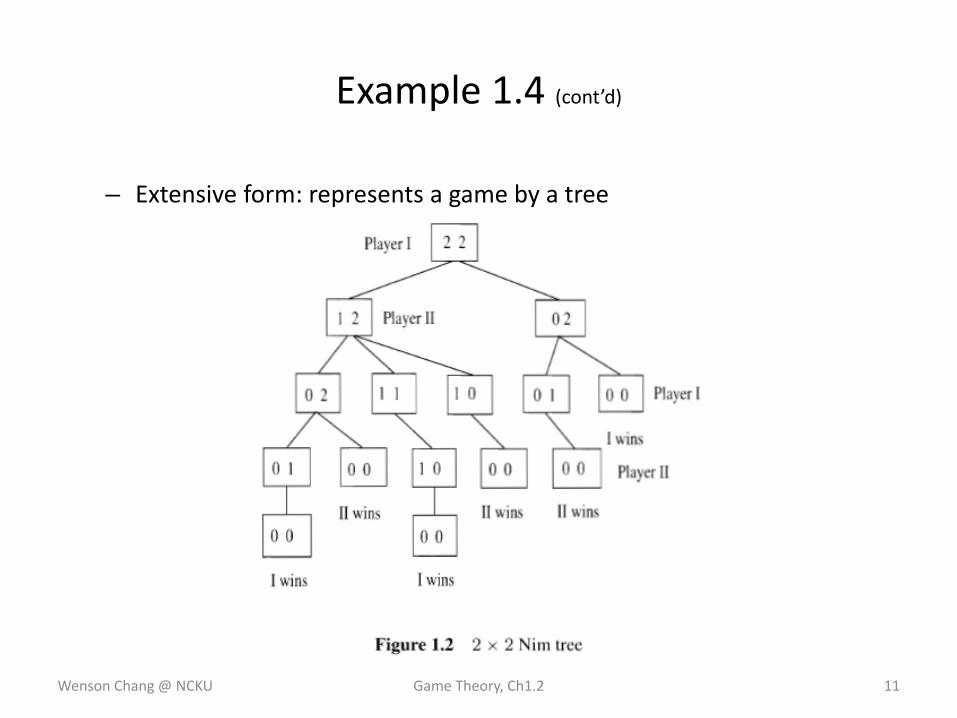
– Extensive form: represents a game by a tree
Wenson Chang @ NCKU Game Theory, Ch1.2 11
Example 1.4 (cont’d)
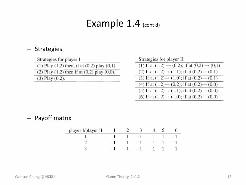
– Strategies
– Payoff matrix
Wenson Chang @ NCKU Game Theory, Ch1.2 12
Example 1.4 (cont’d)
• Analysis of 2 × 2 Nim.– Any rational player in II’s position would drop column 5 In the payoff
matrix from consideration (column 5 is called a dominated strategy).
By the same token, player I would drop column 3 from consideration.
– The value of this game is ‐1 and the strategies are saddle points, or optimal strategies for the players.
• Player I can improve the payoff if player II deviates from column 3.
• There are three saddle points in this example, so saddles are not necessarily unique.
Wenson Chang @ NCKU Game Theory, Ch1.2 13
Example 1.4 (cont’d)
• Russian roulette– Two players are faced with a six‐shot pistol loaded with one bullet.
– The players ante $1000, and player I goes first.
– At each play of the game, a player has the option of putting an additional $1000 into the pot and passing, or spinning the chamber and firing (at his own head).
Wenson Chang @ NCKU Game Theory, Ch1.2 14
Example 1.5
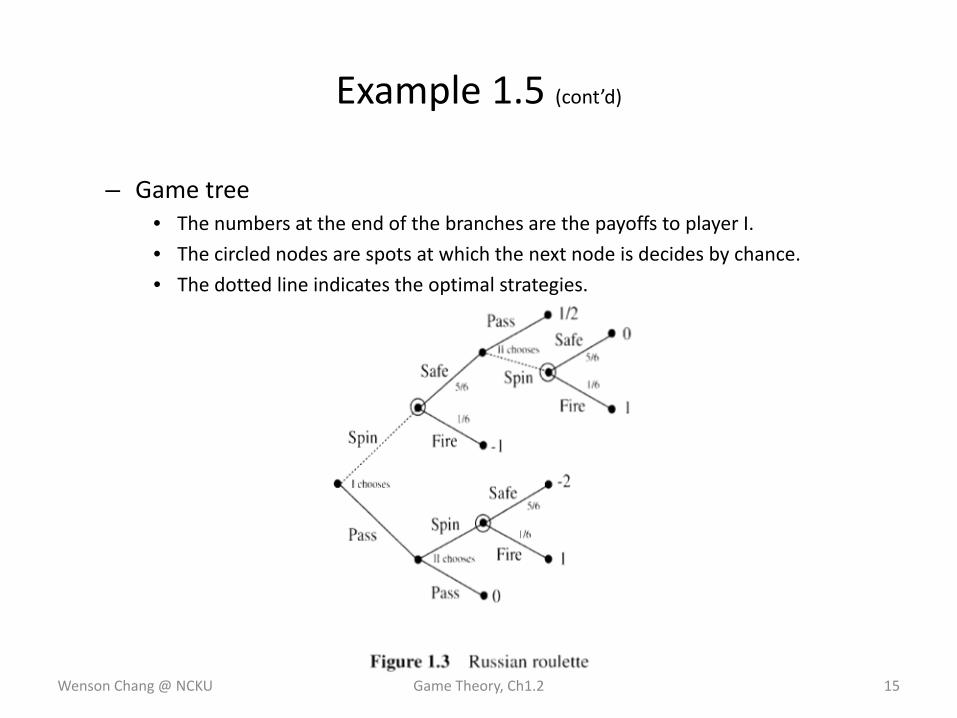
– Game tree• The numbers at the end of the branches are the payoffs to player I.
• The circled nodes are spots at which the next node is decides by chance.
• The dotted line indicates the optimal strategies.
Wenson Chang @ NCKU Game Theory, Ch1.2 15
Example 1.5 (cont’d)
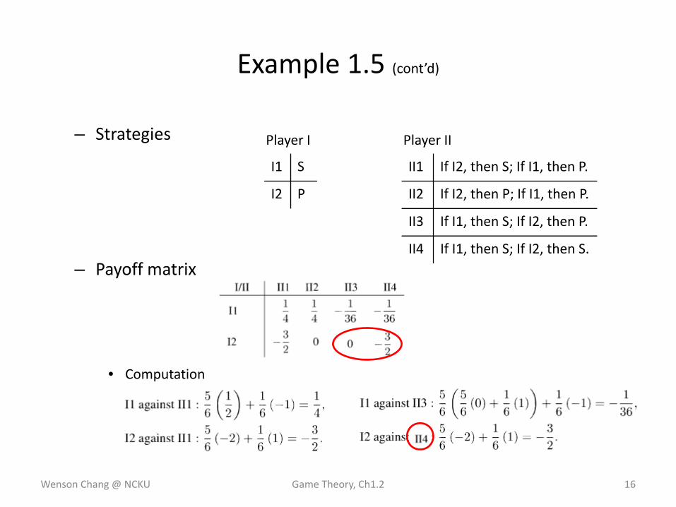
– Strategies
– Payoff matrix
• Computation
Wenson Chang @ NCKU Game Theory, Ch1.2 16
Example 1.5 (cont’d)
I1 S
I2 P
II1 If I2, then S; If I1, then P.
II2 If I2, then P; If I1, then P.
II3 If I1, then S; If I2, then P.
II4 If I1, then S; If I2, then S.
Player I Player II
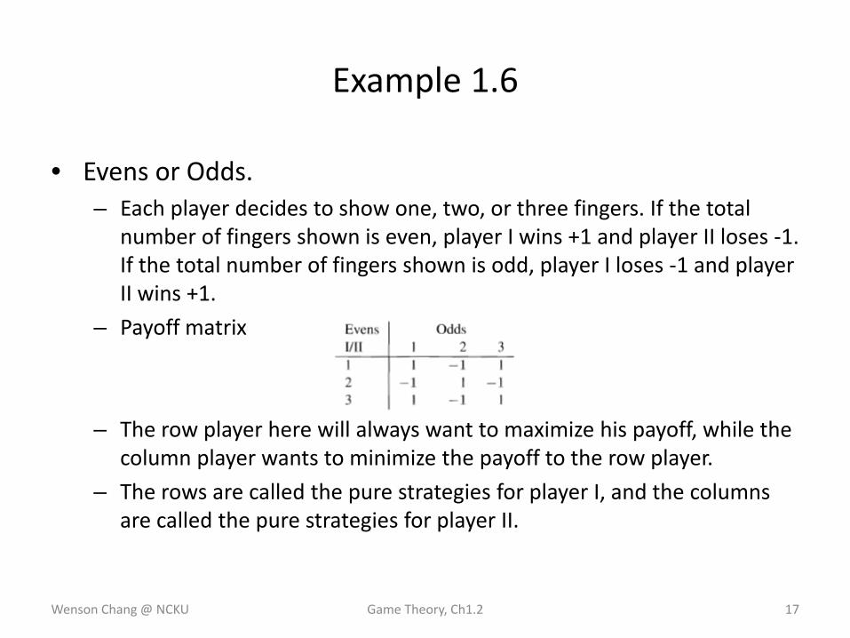
• Evens or Odds.– Each player decides to show one, two, or three fingers. If the total
number of fingers shown is even, player I wins +1 and player II loses ‐1. If the total number of fingers shown is odd, player I loses ‐1 and player II wins +1.
– Payoff matrix
– The row player here will always want to maximize his payoff, while the column player wants to minimize the payoff to the row player.
– The rows are called the pure strategies for player I, and the columns are called the pure strategies for player II.
Wenson Chang @ NCKU Game Theory, Ch1.2 17
Example 1.6
Example 1.6 (cont’d)
– If a player always plays the same strategy, the opposing player can win the game.
– It seems that the only alternatives is for the players to mix up their strategies and play some rows and columns sometimes and other rows and columns at other times.
Wenson Chang @ NCKU Game Theory, Ch1.2 18
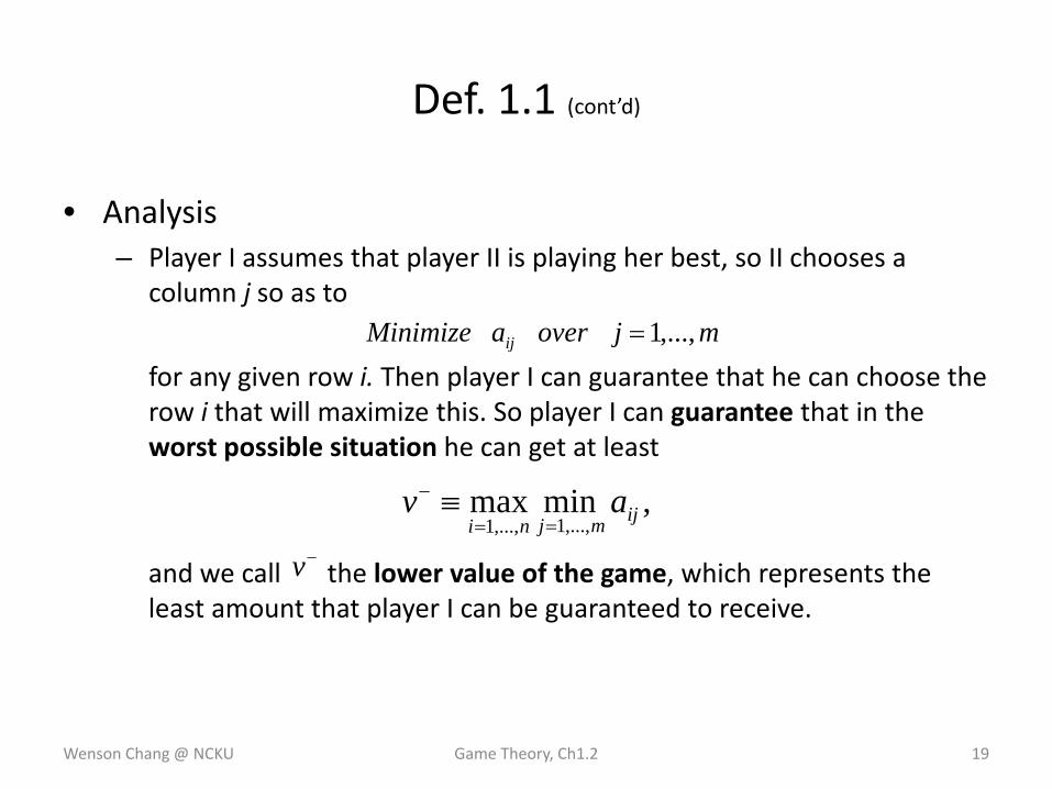
• Analysis– Player I assumes that player II is playing her best, so II chooses a
column j so as to
for any given row i. Then player I can guarantee that he can choose the row i that will maximize this. So player I can guarantee that in the worst possible situation he can get at least
and we call the lower value of the game, which represents the least amount that player I can be guaranteed to receive.
Wenson Chang @ NCKU Game Theory, Ch1.2 19
Def. 1.1 (cont’d)
mjoveraMinimize ij ,...,1=
,minmax,...,1,...,1 ijmjni
av==
− ≡−v
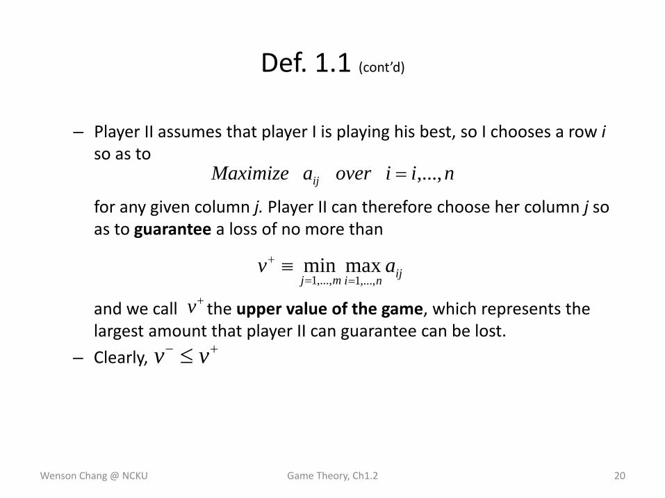
– Player II assumes that player I is playing his best, so I chooses a row i so as to
for any given column j. Player II can therefore choose her column j so as to guarantee a loss of no more than
and we call the upper value of the game, which represents the largest amount that player II can guarantee can be lost.
– Clearly,
Wenson Chang @ NCKU Game Theory, Ch1.2 20
Def. 1.1 (cont’d)
niioveraMaximize ij ,...,=
ijnimjav
,...,1,...,1maxmin==
+ ≡
+v
+− ≤ vv
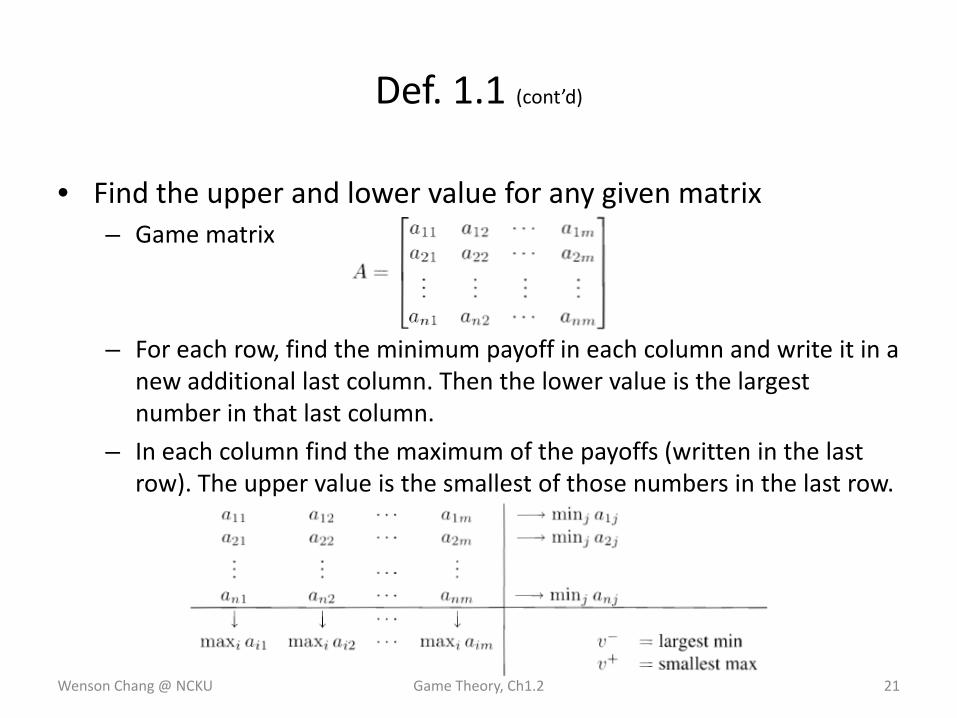
• Find the upper and lower value for any given matrix– Game matrix
– For each row, find the minimum payoff in each column and write it in a new additional last column. Then the lower value is the largest number in that last column.
– In each column find the maximum of the payoffs (written in the last row). The upper value is the smallest of those numbers in the last row.
Wenson Chang @ NCKU Game Theory, Ch1.2 21
Def. 1.1 (cont’d)
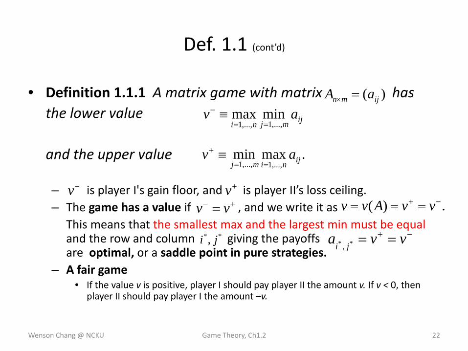
• Definition 1.1.1 A matrix game with matrix has the lower value
and the upper value
– is player I's gain floor, and is player II’s loss ceiling.– The game has a value if , and we write it as
This means that the smallest max and the largest min must be equal and the row and column giving the payoffs are optimal, or a saddle point in pure strategies.
– A fair game• If the value v is positive, player I should pay player II the amount v. If v < 0, then
player II should pay player I the amount –v.
Wenson Chang @ NCKU Game Theory, Ch1.2 22
Def. 1.1 (cont’d)
)( ijmn aA =×
ijmjniav
,...,1,...,1minmax==
− ≡
.maxmin,...,1,...,1 ijnimj
av==
+ ≡
−v +v+− = vv .)( −+ === vvAvv
**, ji −+ == vva ji ** ,
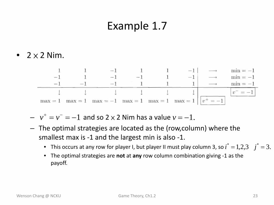
• 2 × 2 Nim.
– and so 2 × 2 Nim has a value
– The optimal strategies are located as the (row,column) where the smallest max is ‐1 and the largest min is also ‐1.
• This occurs at any row for player I, but player II must play column 3, so
• The optimal strategies are not at any row column combination giving ‐1 as the payoff.
Wenson Chang @ NCKU Game Theory, Ch1.2 23
Example 1.7
1−== −+ vv .1−=v
.33,2,1 ** == ji
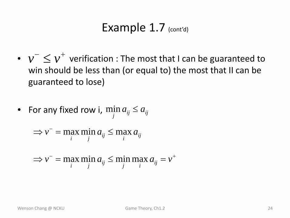
• verification : The most that I can be guaranteed to win should be less than (or equal to) the most that II can be guaranteed to lose)
• For any fixed row i,
Wenson Chang @ NCKU Game Theory, Ch1.2 24
Example 1.7 (cont’d)
+− ≤ vv
ijijjaa ≤min
ijiijjiaav maxminmax ≤=⇒ −
+− =≤=⇒ vaav ijijijjimaxminminmax
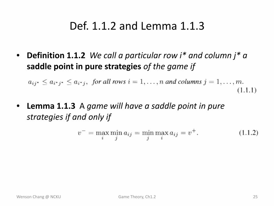
• Definition 1.1.2 We call a particular row i* and column j* a saddle point in pure strategies of the game if
• Lemma 1.1.3 A game will have a saddle point in pure strategies if and only if
Wenson Chang @ NCKU Game Theory, Ch1.2 25
Def. 1.1.2 and Lemma 1.1.3
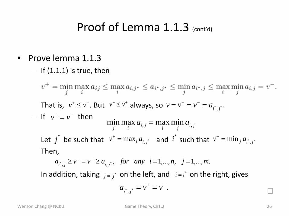
• Prove lemma 1.1.3– If (1.1.1) is true, then
That is, . But always, so
– If then
Let be such that and such that
Then,
In addition, taking on the left, and on the right, gives
Wenson Chang @ NCKU Game Theory, Ch1.2 26
Proof of Lemma 1.1.3 (cont’d)
−+ ≤ vv +− ≤ vv .** , jiavvv === −+
−+ = vvjijijiij
aa ,, minmaxmaxmin =
*j *,max jii av =+ *i .min ,* jij av =−
.,...,1,,...,1,** ,, mjnianyforavva jiji ==≥=≥ +−
*jj = *ii =
.** ,−+ == vva ji
• When a saddle point exists in pure strategies, (1.1.1) says that if any player deviates from playing her part of the saddle, then the other player can take advantage and improve his payoff.
• Each part of a saddle is a best response to the other.
Wenson Chang @ NCKU Game Theory, Ch1.2 27
Best Reponse (cont’d)
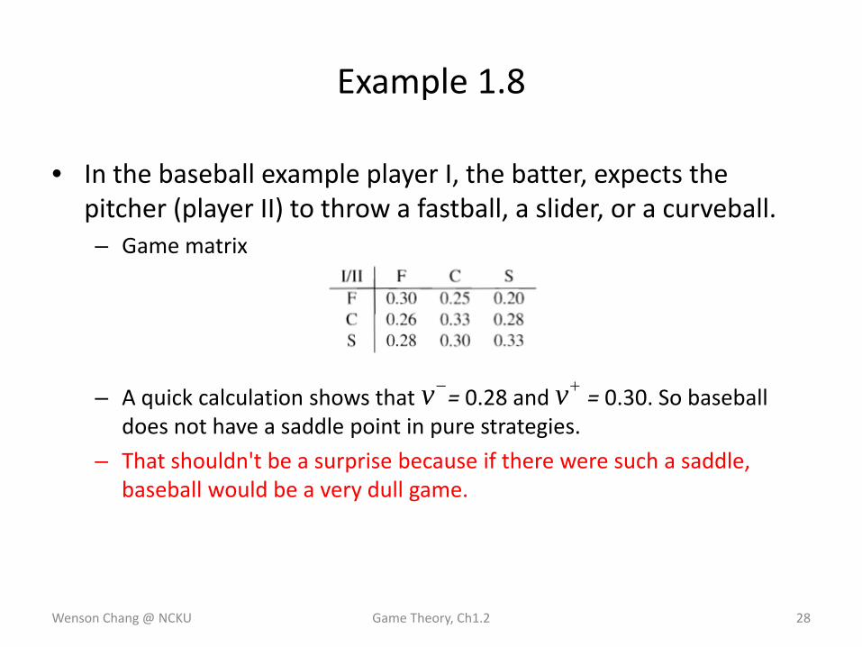
• In the baseball example player I, the batter, expects the pitcher (player II) to throw a fastball, a slider, or a curveball. – Game matrix
– A quick calculation shows that = 0.28 and = 0.30. So baseball does not have a saddle point in pure strategies.
– That shouldn't be a surprise because if there were such a saddle, baseball would be a very dull game.
Wenson Chang @ NCKU Game Theory, Ch1.2 28
Example 1.8
−v +v
Find the Upper and Lower Values With Maple
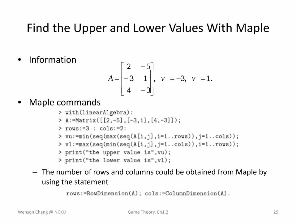
• Information
• Maple commands
– The number of rows and columns could be obtained from Maple by using the statement
Wenson Chang @ NCKU Game Theory, Ch1.2 29
.1,3,34
1352
=−=⎥⎥⎥
⎦
⎤
⎢⎢⎢
⎣
⎡
−−
−= +− vvA
The Von Neumann Minimax Theorem
Wenson Chang @ NCKU Game Theory, Ch1.2 30
Mixed Strategies
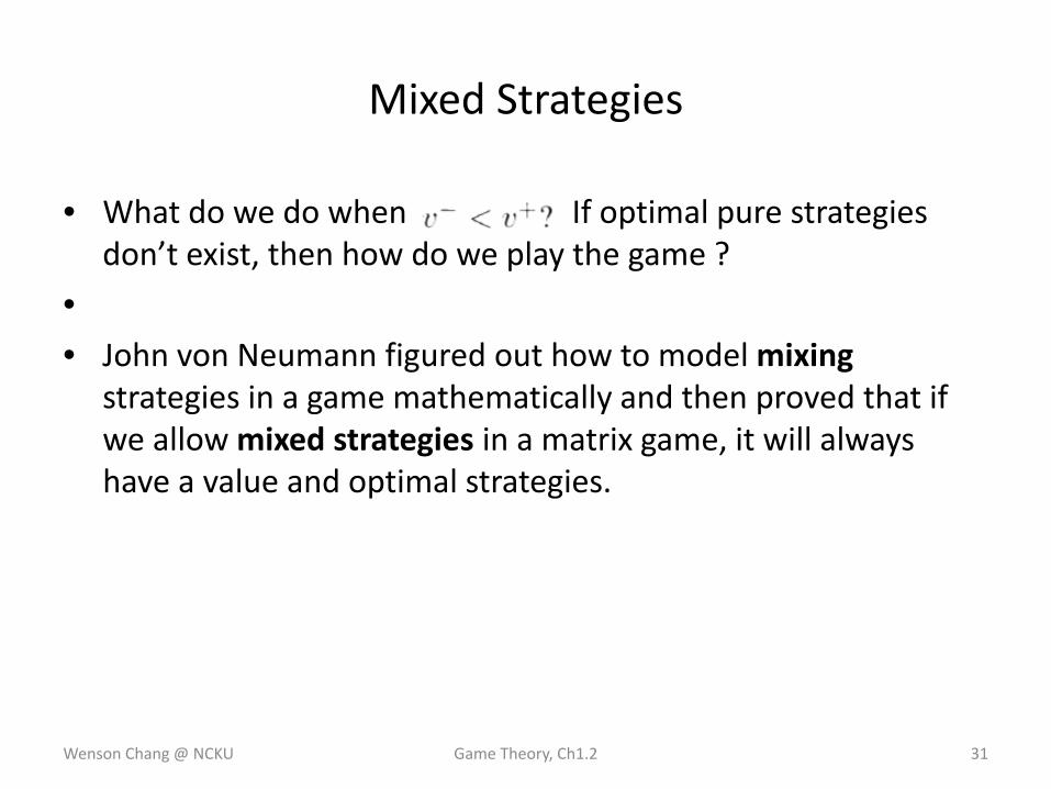
• What do we do when If optimal pure strategies don’t exist, then how do we play the game ?
•• John von Neumann figured out how to model mixing
strategies in a game mathematically and then proved that if we allow mixed strategies in a matrix game, it will always have a value and optimal strategies.
Wenson Chang @ NCKU Game Theory, Ch1.2 31
Def. 1.2.1
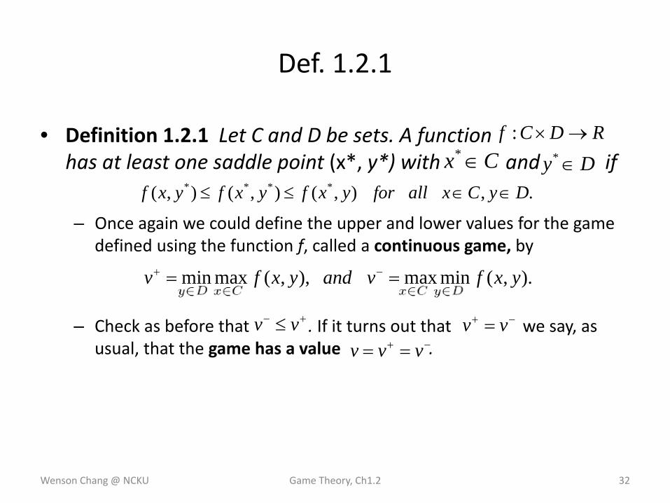
• Definition 1.2.1 Let C and D be sets. A function has at least one saddle point (x*, y*) with and if
– Once again we could define the upper and lower values for the game defined using the function f, called a continuous game, by
– Check as before that . If it turns out that we say, as usual, that the game has a value .
Wenson Chang @ NCKU Game Theory, Ch1.2 32
RDCf →×:Cx ∈* Dy ∈*
.,),(),(),( **** DyCxallforyxfyxfyxf ∈∈≤≤
).,(minmax),,(maxmin yxfvandyxfvCxDyDyCx ∈∈
−
∈∈
+ ==
+− ≤ vv −+ = vv−+ == vvv
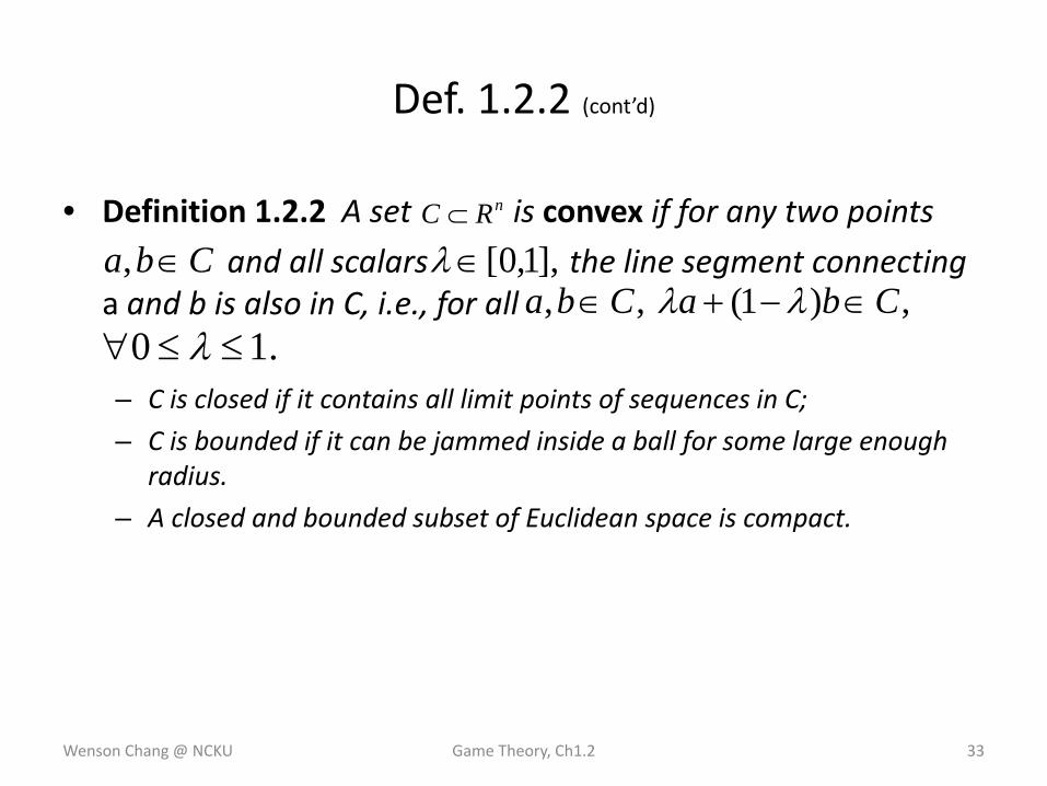
• Definition 1.2.2 A set is convex if for any two points
and all scalars the line segment connecting a and b is also in C, i.e., for all
– C is closed if it contains all limit points of sequences in C;
– C is bounded if it can be jammed inside a ball for some large enough radius.
– A closed and bounded subset of Euclidean space is compact.
Wenson Chang @ NCKU Game Theory, Ch1.2 33
Def. 1.2.2 (cont’d)
nRC ⊂
Cba ∈, ],1,0[∈λ,, Cba ∈ ,)1( Cba ∈−+ λλ
.10 ≤≤∀ λ
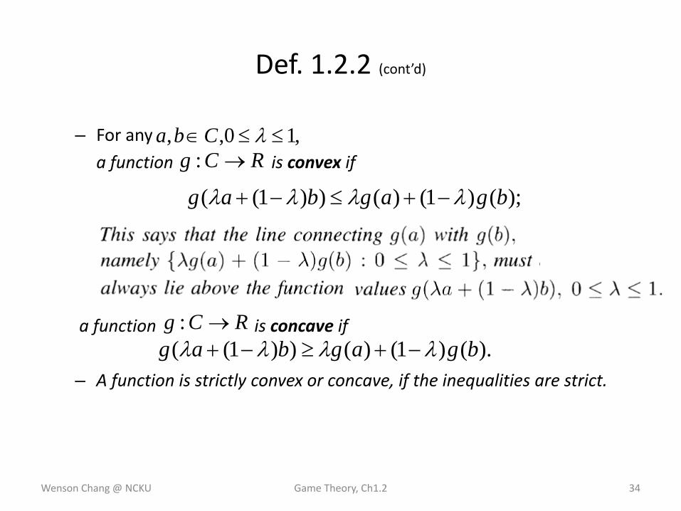
– For any
a function is convex if
a function is concave if
– A function is strictly convex or concave, if the inequalities are strict.
Wenson Chang @ NCKU Game Theory, Ch1.2 34
Def. 1.2.2 (cont’d)
,10,, ≤≤∈ λCbaRCg →:
);()1()())1(( bgagbag λλλλ −+≤−+
RCg →:).()1()())1(( bgagbag λλλλ −+≥−+
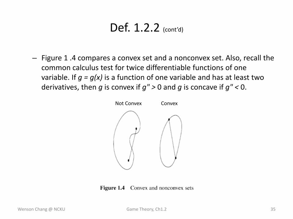
– Figure 1 .4 compares a convex set and a nonconvex set. Also, recall the common calculus test for twice differentiable functions of one variable. If g = g(x) is a function of one variable and has at least two derivatives, then g is convex if g" > 0 and g is concave if g" < 0.
Wenson Chang @ NCKU Game Theory, Ch1.2 35
Def. 1.2.2 (cont’d)
Not Convex Convex
• Theorem 1.2.3 Let be a continuous function. Let
and be convex, closed, and bounded. Suppose that is concave and is convex. Then
– For example,
This function has so it is convex in y for each x and concave in x for each y.
– Since and the square is closed and bounded, von Neumann's theorem guarantees the existence of a saddle point for this function.
Wenson Chang @ NCKU Game Theory, Ch1.2 36
The Von Neumann Minimax Theorem (cont’d)
RDCf →×:nRC∈ mRD∈
),( yxfx a ),( yxfy a−
∈∈∈∈
+ === vyxfyxfvDyCxCxDy
),(minmax),(maxmin
.1,01224),( ≤≤+−−= yxonyxxyyxf,00,00 ≤=≥= yyxx ff
],1,0[]1,0[),( ×∈yx
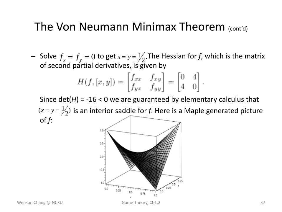
– Solve to get The Hessian for f, which is the matrix of second partial derivatives, is given by
Since det(H) = ‐16 < 0 we are guaranteed by elementary calculus that
is an interior saddle for f. Here is a Maple generated picture of f:
Wenson Chang @ NCKU Game Theory, Ch1.2 37
The Von Neumann Minimax Theorem (cont’d)
0== yx ff .21== yx
)21( == yx
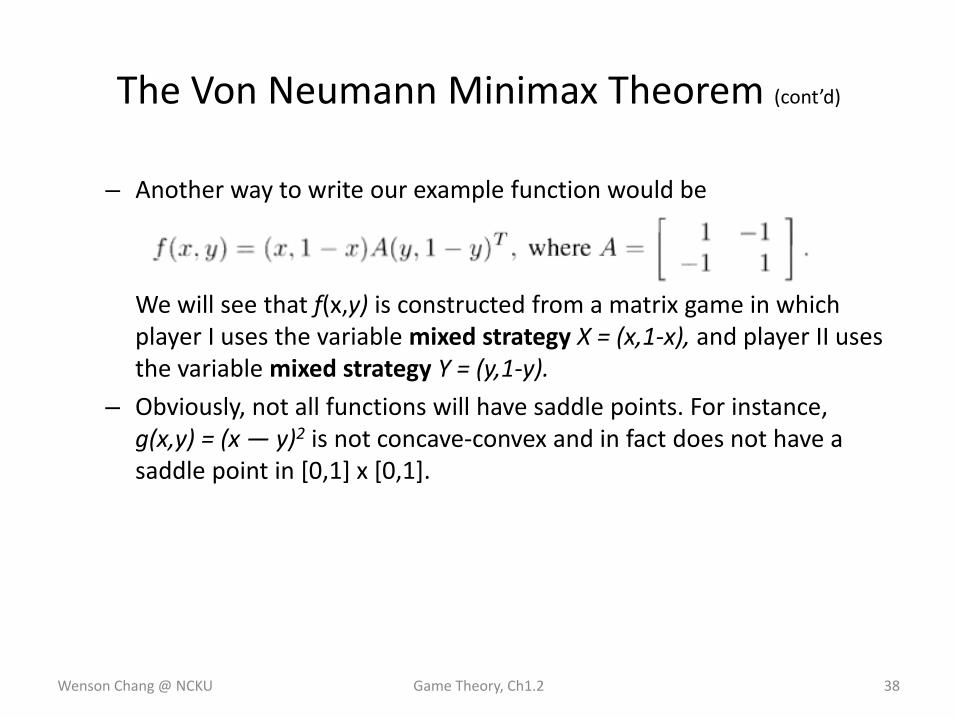
– Another way to write our example function would be
We will see that f(x,y) is constructed from a matrix game in which player I uses the variable mixed strategy X = (x,1‐x), and player II uses the variable mixed strategy Y = (y,1‐y).
– Obviously, not all functions will have saddle points. For instance, g(x,y) = (x — y)2 is not concave‐convex and in fact does not have a saddle point in [0,1] x [0,1].
Wenson Chang @ NCKU Game Theory, Ch1.2 38
The Von Neumann Minimax Theorem (cont’d)
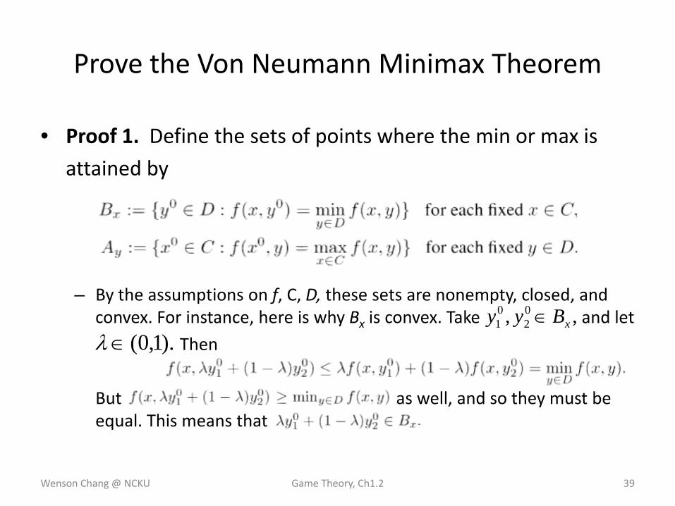
• Proof 1. Define the sets of points where the min or max is
attained by
– By the assumptions on f, C, D, these sets are nonempty, closed, and convex. For instance, here is why Bx is convex. Take and let
Then
But as well, and so they must be equal. This means that
Wenson Chang @ NCKU Game Theory, Ch1.2 39
Prove the Von Neumann Minimax Theorem
,, 02
01 xByy ∈
).1,0(∈λ
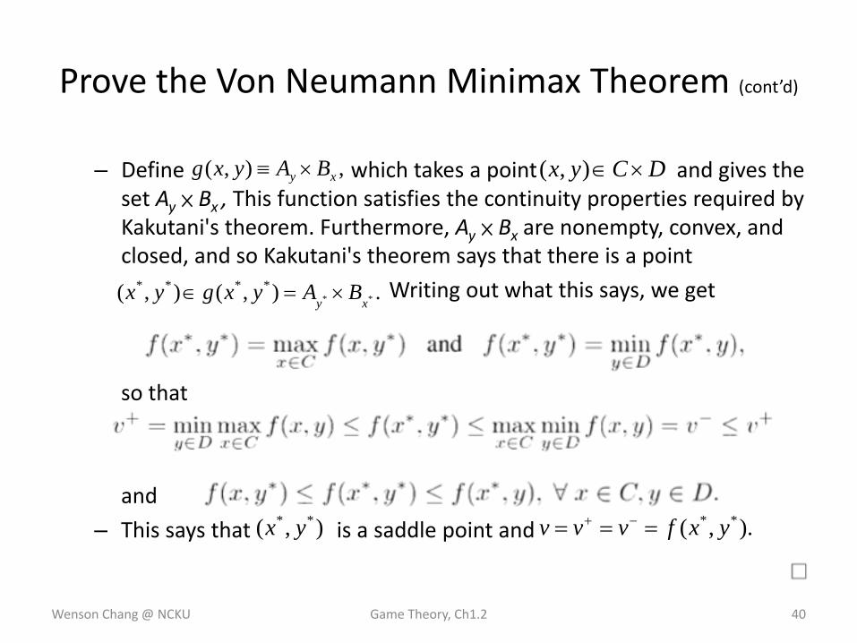
– Define which takes a point and gives the set Ay × Bx , This function satisfies the continuity properties required by Kakutani's theorem. Furthermore, Ay × Bx are nonempty, convex, and closed, and so Kakutani's theorem says that there is a point
Writing out what this says, we get
so that
and
– This says that is a saddle point and
Wenson Chang @ NCKU Game Theory, Ch1.2 40
Prove the Von Neumann Minimax Theorem (cont’d)
,),( xy BAyxg ×≡ DCyx ×∈),(
.),(),( ******
xy BAyxgyx ×=∈
).,( ** yxfvvv === −+),( ** yx
Kakutani's Theorem
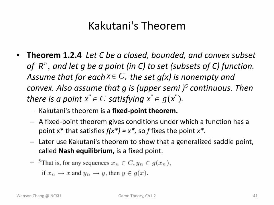
• Theorem 1.2.4 Let C be a closed, bounded, and convex subset of and let g be a point (in C) to set (subsets of C) function. Assume that for each the set g(x) is nonempty and convex. Also assume that g is (upper semi )5 continuous. Then there is a point satisfying– Kakutani's theorem is a fixed‐point theorem.
– A fixed‐point theorem gives conditions under which a function has a point x* that satisfies f(x*) = x*, so f fixes the point x*.
– Later use Kakutani's theorem to show that a generalized saddle point, called Nash equilibrium, is a fixed point.
–
Wenson Chang @ NCKU Game Theory, Ch1.2 41
,nR,Cx∈
Cx ∈* ).( ** xgx ∈
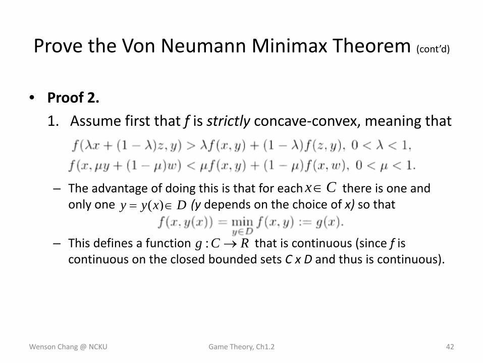
• Proof 2.
1. Assume first that f is strictly concave‐convex, meaning that
– The advantage of doing this is that for each there is one and only one (y depends on the choice of x) so that
– This defines a function that is continuous (since f is continuous on the closed bounded sets C x D and thus is continuous).
Wenson Chang @ NCKU Game Theory, Ch1.2 42
Prove the Von Neumann Minimax Theorem (cont’d)
Cx∈Dxyy ∈= )(
RCg →:
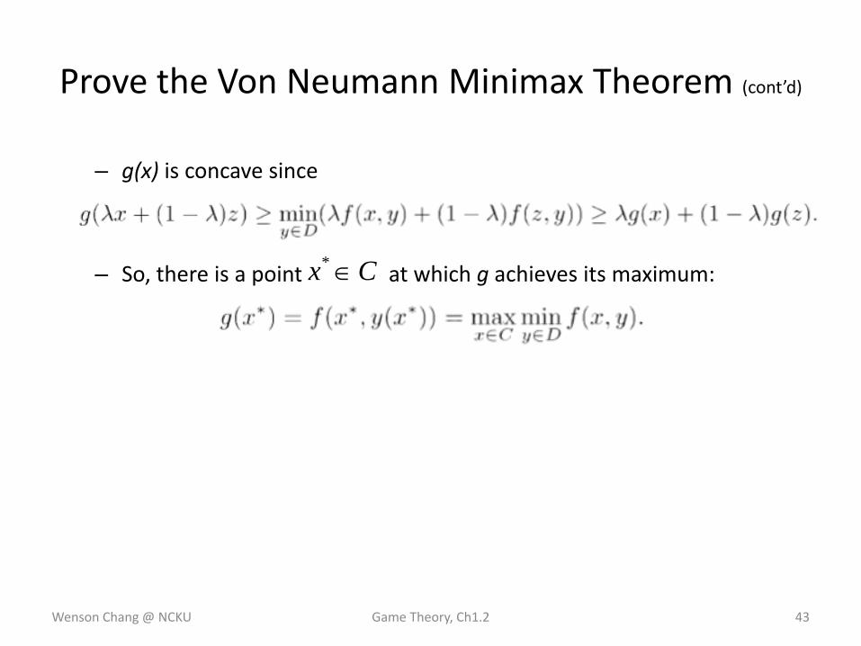
– g(x) is concave since
– So, there is a point at which g achieves its maximum:
Wenson Chang @ NCKU Game Theory, Ch1.2 43
Prove the Von Neumann Minimax Theorem (cont’d)
Cx ∈*
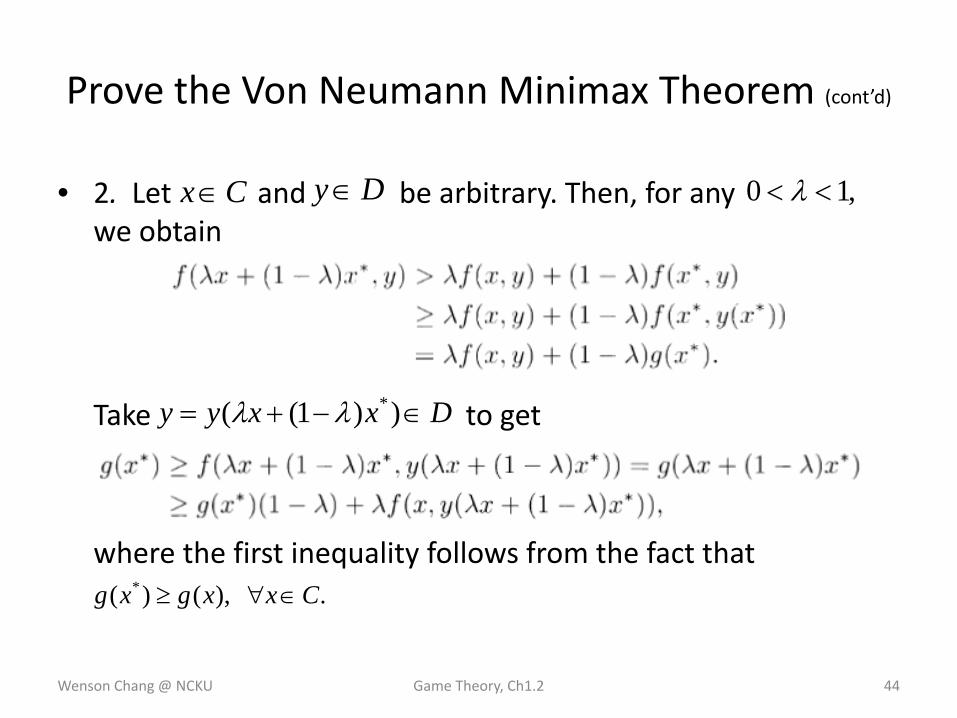
• 2. Let and be arbitrary. Then, for any we obtain
Take to get
where the first inequality follows from the fact that
Wenson Chang @ NCKU Game Theory, Ch1.2 44
Prove the Von Neumann Minimax Theorem (cont’d)
Cx∈ Dy∈ ,10 << λ
Dxxyy ∈−+= ))1(( *λλ
.),()( * Cxxgxg ∈∀≥
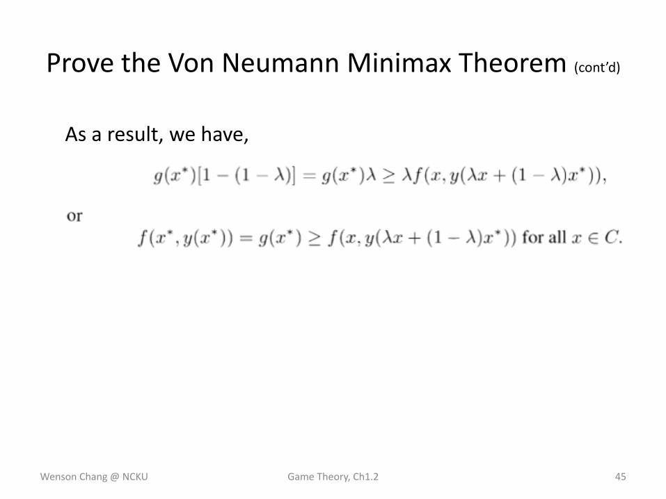
As a result, we have,
Wenson Chang @ NCKU Game Theory, Ch1.2 45
Prove the Von Neumann Minimax Theorem (cont’d)
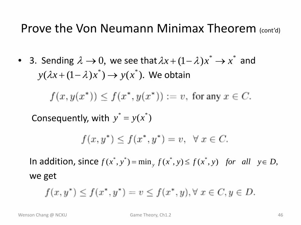
• 3. Sending we see that and
We obtain
Consequently, with
In addition, since
we get
Wenson Chang @ NCKU Game Theory, Ch1.2 46
Prove the Von Neumann Minimax Theorem (cont’d)
,0→λ **)1( xxx →−+ λλ).())1(( ** xyxxy →−+ λλ
)( ** xyy =
,),(),(min),( **** Dyallforyxfyxfyxf y ∈≤=
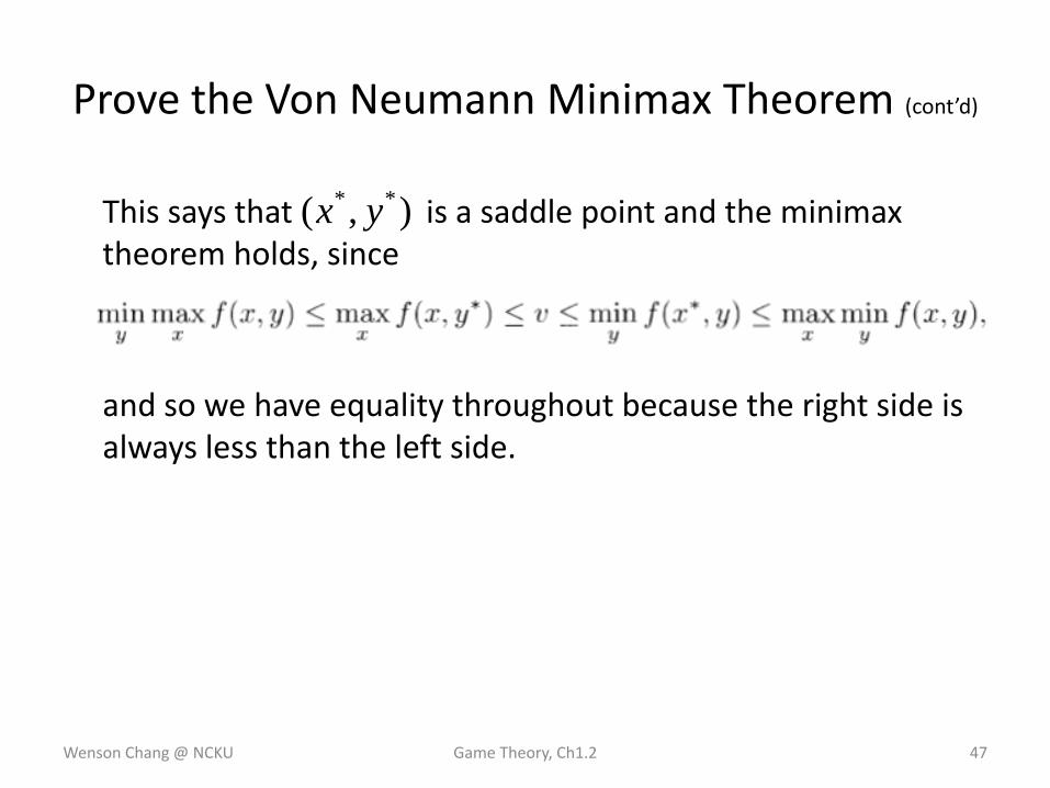
This says that is a saddle point and the minimaxtheorem holds, since
and so we have equality throughout because the right side is always less than the left side.
Wenson Chang @ NCKU Game Theory, Ch1.2 47
Prove the Von Neumann Minimax Theorem (cont’d)
),( ** yx
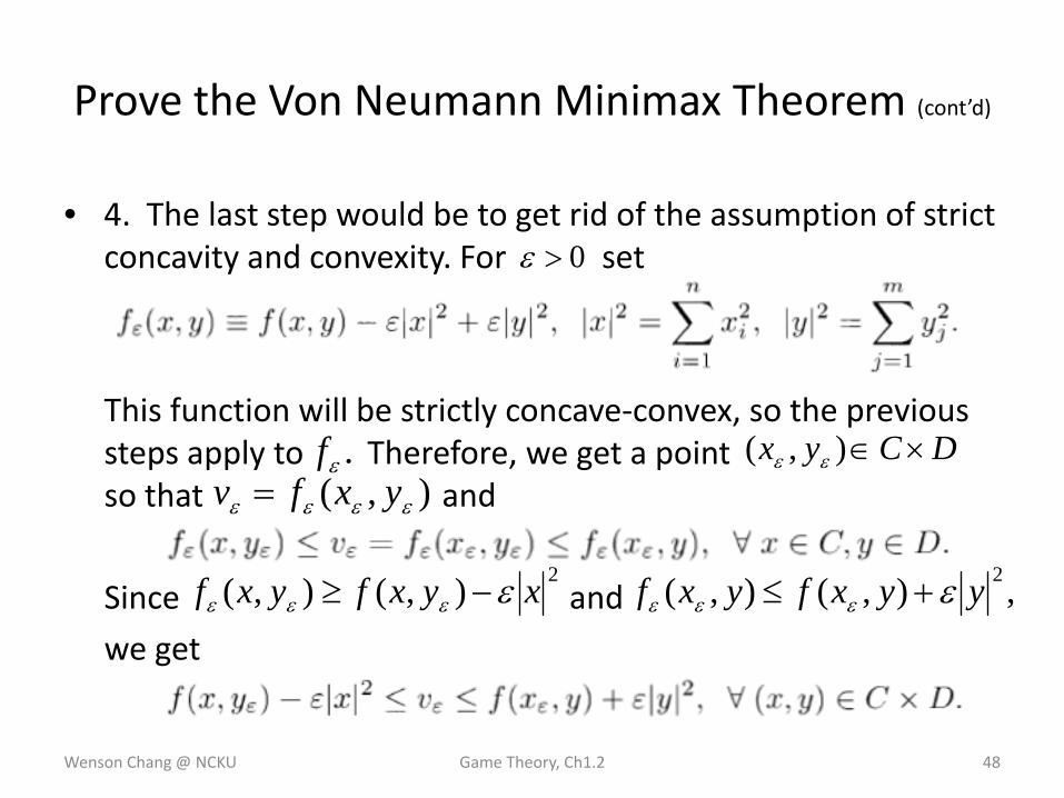
• 4. The last step would be to get rid of the assumption of strict concavity and convexity. For set
This function will be strictly concave‐convex, so the previous steps apply to Therefore, we get a point so that and
Since and
we get
Wenson Chang @ NCKU Game Theory, Ch1.2 48
Prove the Von Neumann Minimax Theorem (cont’d)
0>ε
.εf DCyx ×∈),( εε
),( εεεε yxfv =
2),(),( xyxfyxf εεεε −≥ ,),(),( 2yyxfyxf εεεε +≤
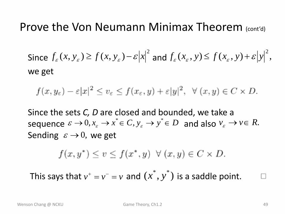
Since and
we get
Since the sets C, D are closed and bounded, we take a sequence and also Sending we get
This says that and is a saddle point.
Wenson Chang @ NCKU Game Theory, Ch1.2 49
Prove the Von Neumann Minimax Theorem (cont’d)
2),(),( xyxfyxf εεεε −≥ ,),(),( 2yyxfyxf εεεε +≤
DyyCxx ∈→∈→→ ** ,,0 εεε .Rvv ∈→ε
,0→ε
vvv == −+ ),( ** yx
The Von Neumann Minimax Theorem (cont’d)
• Von Neumann's theorem tells us what we need in order to guarantee that our game has a value.
• It is critical that we are dealing with a concave‐convex function, and that the strategy sets be convex.
Wenson Chang @ NCKU Game Theory, Ch1.2 50
Mixed Strategies
Wenson Chang @ NCKU Game Theory, Ch1.2 51
Mixed Strategies
• Von Neumann’s theorem suggests that: we need convexity of the sets of strategies, whatever they may be, and convexity‐concavity of the payoff function, whatever it may be.– A saddle point in pure strategies will not always exist.
• In most two‐person zero sum games a saddle point in pure strategies will not exist because that would say that the players should always do the same thing.
• A player who chooses a pure strategy randomly chooses a row or column according to some probability process that specifies the chance that each pure strategy will be played. These probability vectors are called mixed strategies.
Wenson Chang @ NCKU Game Theory, Ch1.2 52
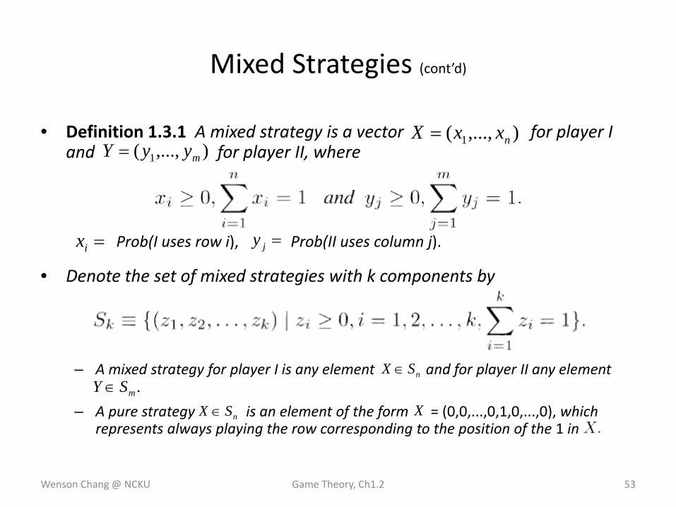
• Definition 1.3.1 A mixed strategy is a vector for player I and for player II, where
• Denote the set of mixed strategies with k components by
– A mixed strategy for player I is any element and for player II any element
– A pure strategy is an element of the form = (0,0,...,0,1,0,...,0), which represents always playing the row corresponding to the position of the 1 in
Wenson Chang @ NCKU Game Theory, Ch1.2 53
Mixed Strategies (cont’d)
),...,( 1 nxxX =),...,( 1 myyY =
=ix =jy
nSX ∈.mSY ∈
nSX ∈ X
Prob(I uses row i), Prob(II uses column j).
Expected Payoff
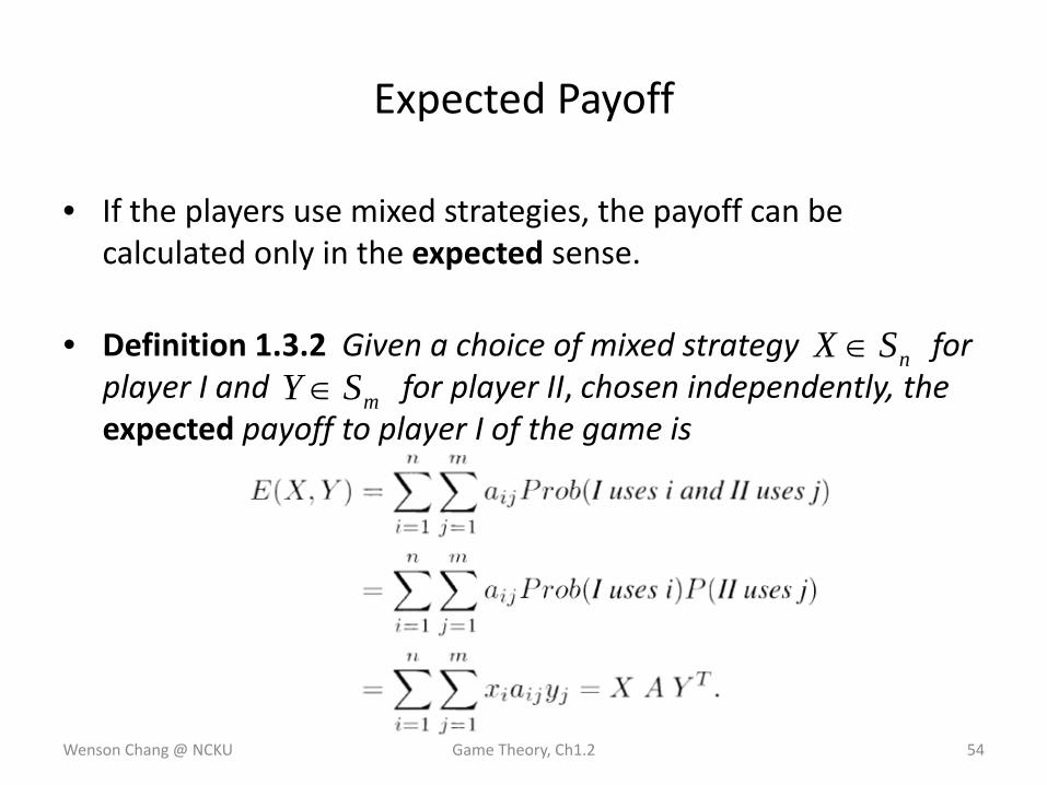
• If the players use mixed strategies, the payoff can be calculated only in the expected sense.
• Definition 1.3.2 Given a choice of mixed strategy for player I and for player II, chosen independently, the expected payoff to player I of the game is
Wenson Chang @ NCKU Game Theory, Ch1.2 54
nSX ∈mSY ∈
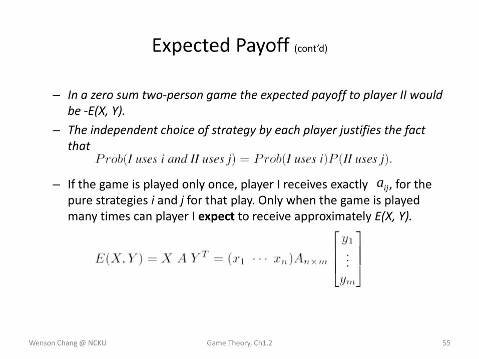
– In a zero sum two‐person game the expected payoff to player II would be ‐E(X, Y).
– The independent choice of strategy by each player justifies the fact that
– If the game is played only once, player I receives exactly , for the pure strategies i and j for that play. Only when the game is played many times can player I expect to receive approximately E(X, Y).
Wenson Chang @ NCKU Game Theory, Ch1.2 55
Expected Payoff (cont’d)
ija
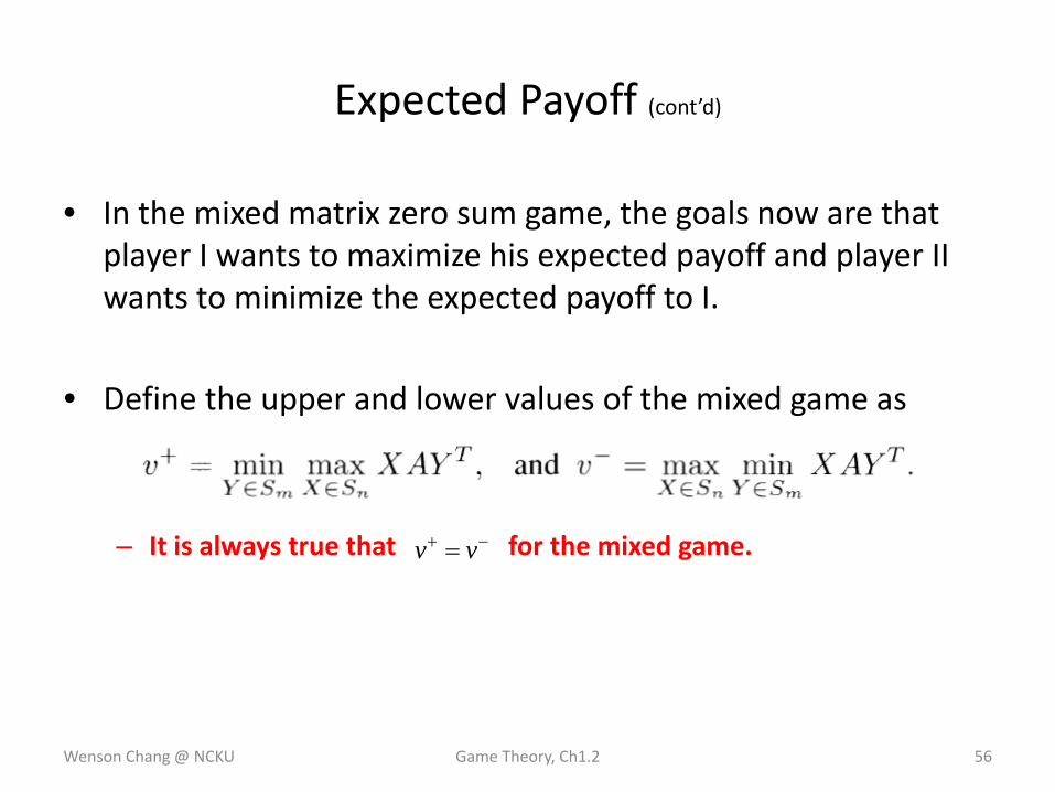
• In the mixed matrix zero sum game, the goals now are that player I wants to maximize his expected payoff and player II wants to minimize the expected payoff to I.
• Define the upper and lower values of the mixed game as
– It is always true that for the mixed game.
Wenson Chang @ NCKU Game Theory, Ch1.2 56
Expected Payoff (cont’d)
−+ = vv
A Saddle Point in Mixed Strategies
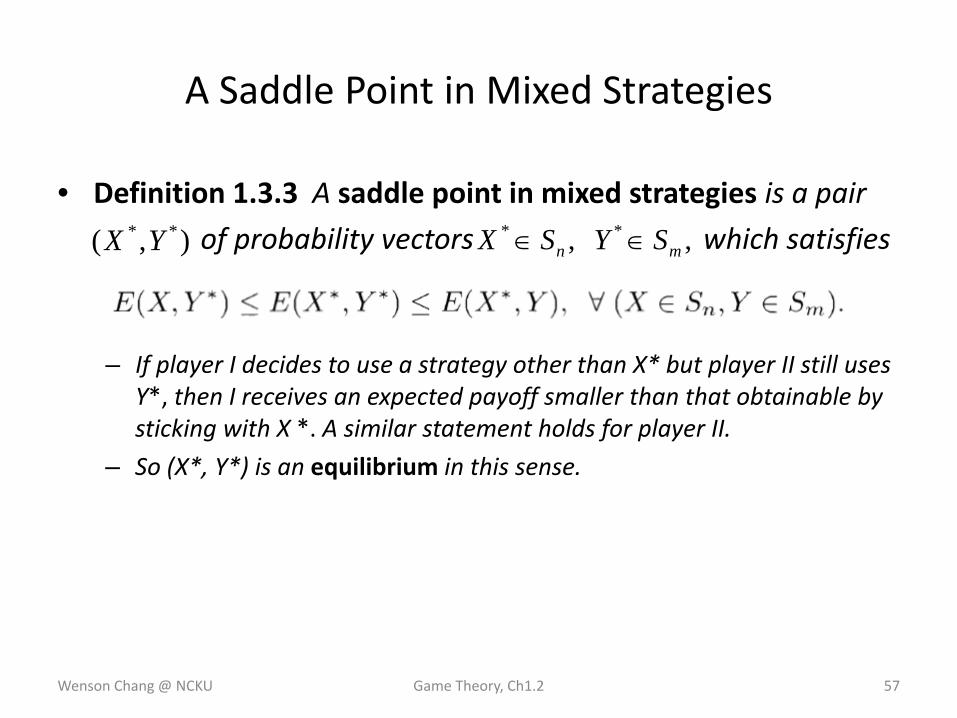
• Definition 1.3.3 A saddle point in mixed strategies is a pair
of probability vectors which satisfies
– If player I decides to use a strategy other than X* but player II still uses Y*, then I receives an expected payoff smaller than that obtainable by sticking with X *. A similar statement holds for player II.
– So (X*, Y*) is an equilibrium in this sense.
Wenson Chang @ NCKU Game Theory, Ch1.2 57
,, **mn SYSX ∈∈),( ** YX
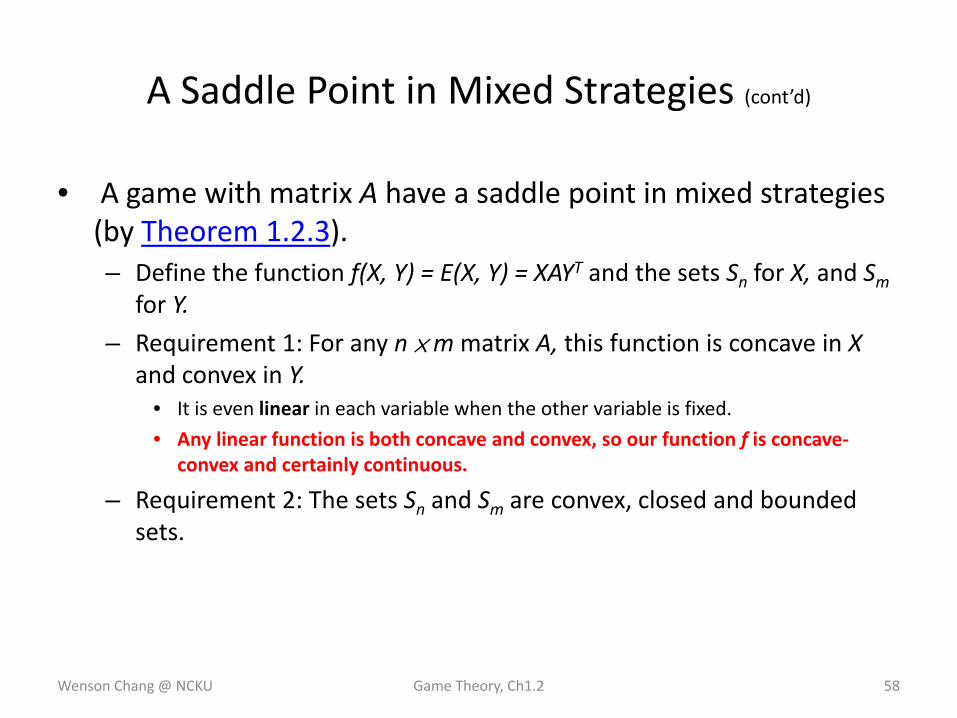
• A game with matrix A have a saddle point in mixed strategies (by Theorem 1.2.3).– Define the function f(X, Y) = E(X, Y) = XAYT and the sets Sn for X, and Sm
for Y.
– Requirement 1: For any n ×m matrix A, this function is concave in X and convex in Y.
• It is even linear in each variable when the other variable is fixed.
• Any linear function is both concave and convex, so our function f is concave‐convex and certainly continuous.
– Requirement 2: The sets Sn and Sm are convex, closed and bounded sets.
Wenson Chang @ NCKU Game Theory, Ch1.2 58
A Saddle Point in Mixed Strategies (cont’d)
The Value of the Game
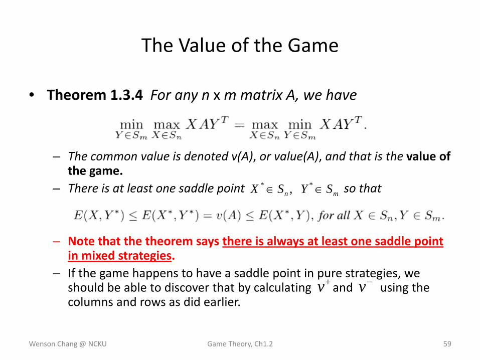
• Theorem 1.3.4 For any n x m matrix A, we have
– The common value is denoted v(A), or value(A), and that is the value of the game.
– There is at least one saddle point so that
– Note that the theorem says there is always at least one saddle point in mixed strategies.
– If the game happens to have a saddle point in pure strategies, we should be able to discover that by calculating and using the columns and rows as did earlier.
Wenson Chang @ NCKU Game Theory, Ch1.2 59
mn SYSX ∈∈ ** ,
−v+v
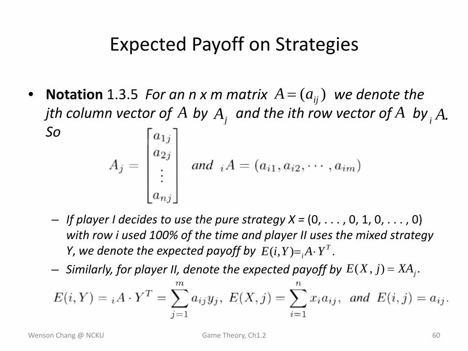
• Notation 1.3.5 For an n x m matrix we denote the jth column vector of by and the ith row vector of by So
– If player I decides to use the pure strategy X = (0, . . . , 0, 1, 0, . . . , 0) with row i used 100% of the time and player II uses the mixed strategy Y, we denote the expected payoff by
– Similarly, for player II, denote the expected payoff by
Wenson Chang @ NCKU Game Theory, Ch1.2 60
)( ijaA =
jAA A .Ai
Expected Payoff on Strategies
.),( Ti YAYiE ⋅=
.),( jXAjXE =
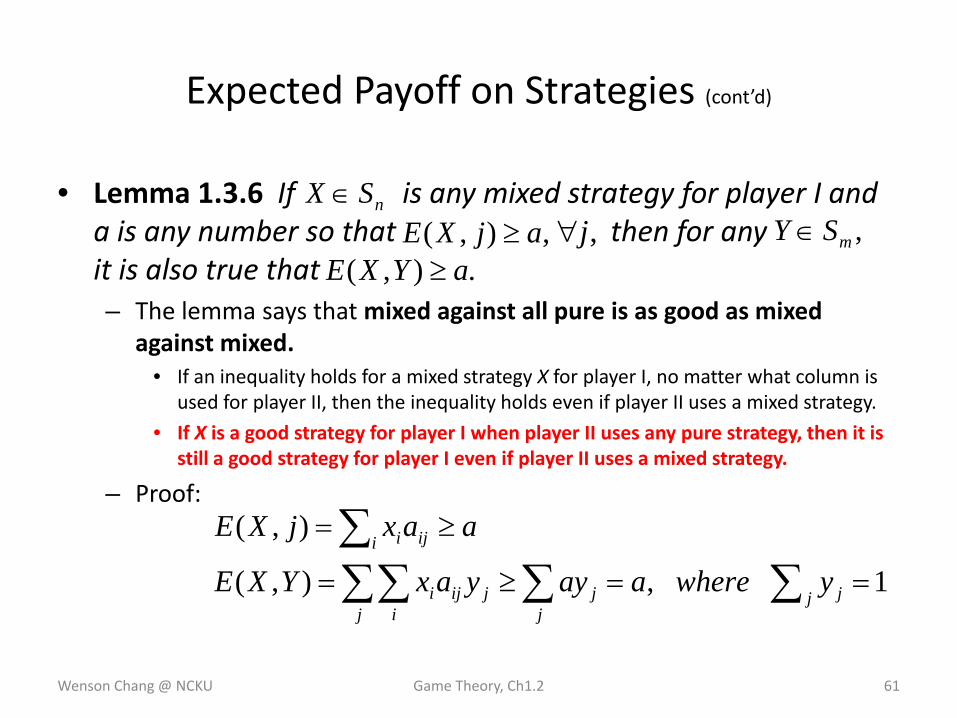
• Lemma 1.3.6 If is any mixed strategy for player I and a is any number so that then for any it is also true that– The lemma says that mixed against all pure is as good as mixed
against mixed.• If an inequality holds for a mixed strategy X for player I, no matter what column is
used for player II, then the inequality holds even if player II uses a mixed strategy.
• If X is a good strategy for player I when player II uses any pure strategy, then it is still a good strategy for player I even if player II uses a mixed strategy.
– Proof:
Wenson Chang @ NCKU Game Theory, Ch1.2 61
Expected Payoff on Strategies (cont’d)
nSX ∈,mSY ∈,),( ajXE ≥ ,j∀
.),( aYXE ≥
aaxjXEi iji ≥=∑),(
1,),( ==≥= ∑∑∑∑ j jj
jj i
jiji ywhereaayyaxYXE
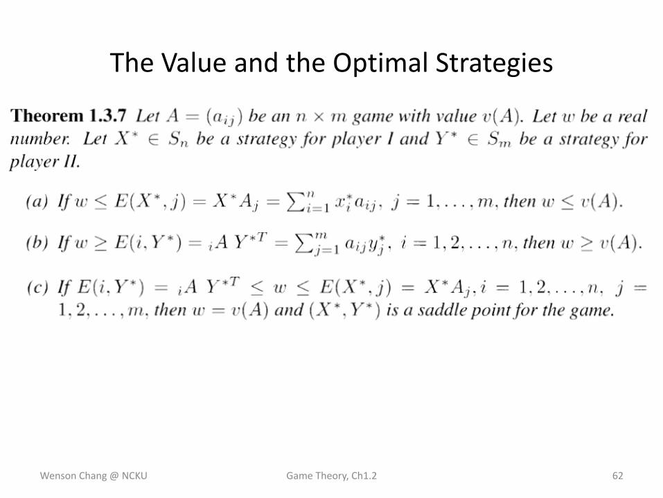
The Value and the Optimal Strategies
Wenson Chang @ NCKU Game Theory, Ch1.2 62
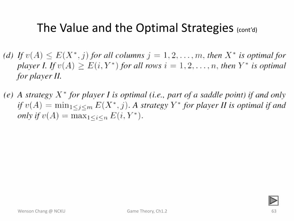
The Value and the Optimal Strategies (cont’d)
Wenson Chang @ NCKU Game Theory, Ch1.2 63
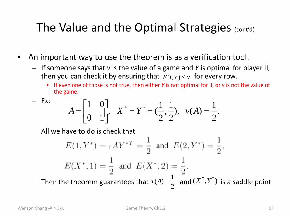
• An important way to use the theorem is as a verification tool.– If someone says that v is the value of a game and Y is optimal for player II,
then you can check it by ensuring that for every row.• If even one of those is not true, then either Y is not optimal for II, or v is not the value of
the game.
– Ex:
All we have to do is check that
Then the theorem guarantees that and is a saddle point.
Wenson Chang @ NCKU Game Theory, Ch1.2 64
The Value and the Optimal Strategies (cont’d)
vYiE ≤),(
.21)(),
21,
21(,
1001 ** ===⎥⎦
⎤⎢⎣
⎡= AvYXA
21)( =Av ),( ** YX
• If we take X=(3/4, 1/4), then E(X,2)=1/4 <1/2, and so, since v=1/2 is the value of the game, we know that X is not optimal for player I.
• Part (c) of the theorem is particularly useful because it gives us a system of inequalities involving v(A), X*, and Y*, which, if we can solve them, will give us the value of the game and the saddle points.
Wenson Chang @ NCKU Game Theory, Ch1.2 65
The Value and the Optimal Strategies (cont’d)
Proof of Theorem 1.3.7 (a) (b)
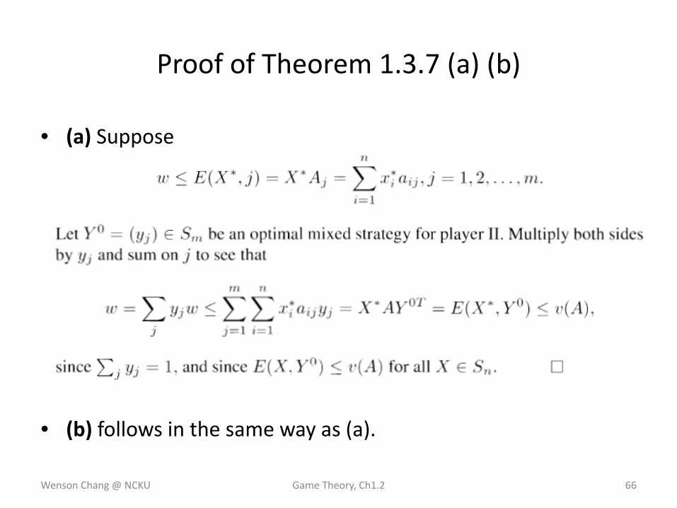
• (a) Suppose
• (b) follows in the same way as (a).
Wenson Chang @ NCKU Game Theory, Ch1.2 66
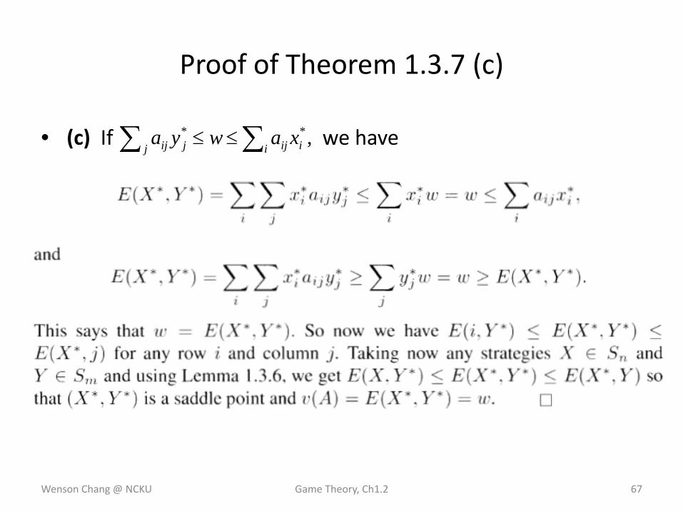
• (c) If we have
Wenson Chang @ NCKU Game Theory, Ch1.2 67
Proof of Theorem 1.3.7 (c)
,** ∑∑ ≤≤i iijj jij xawya
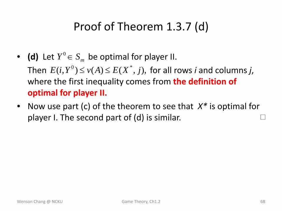
• (d) Let be optimal for player II.
Then for all rows i and columns j, where the first inequality comes from the definition of optimal for player II.
• Now use part (c) of the theorem to see that X* is optimal for player I. The second part of (d) is similar.
Wenson Chang @ NCKU Game Theory, Ch1.2 68
Proof of Theorem 1.3.7 (d)
mSY ∈0
),,()(),( *0 jXEAvYiE ≤≤
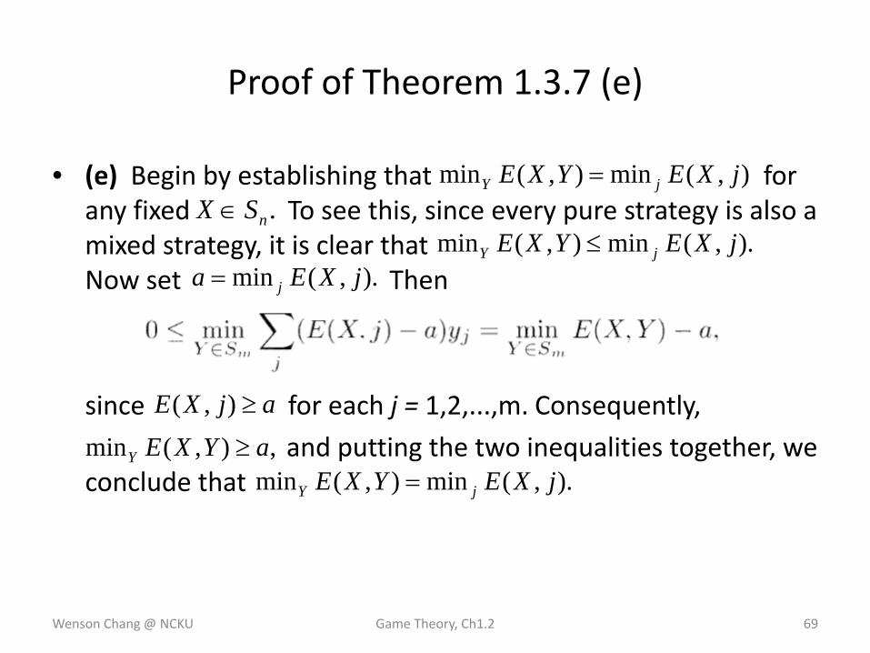
• (e) Begin by establishing that for any fixed To see this, since every pure strategy is also a mixed strategy, it is clear that Now set Then
since for each j = 1,2,...,m. Consequently,
and putting the two inequalities together, we conclude that
Wenson Chang @ NCKU Game Theory, Ch1.2 69
Proof of Theorem 1.3.7 (e)
),(min),(min jXEYXE jY =.nSX ∈
).,(min),(min jXEYXE jY ≤).,(min jXEa j=
ajXE ≥),(,),(min aYXEY ≥
).,(min),(min jXEYXE jY =
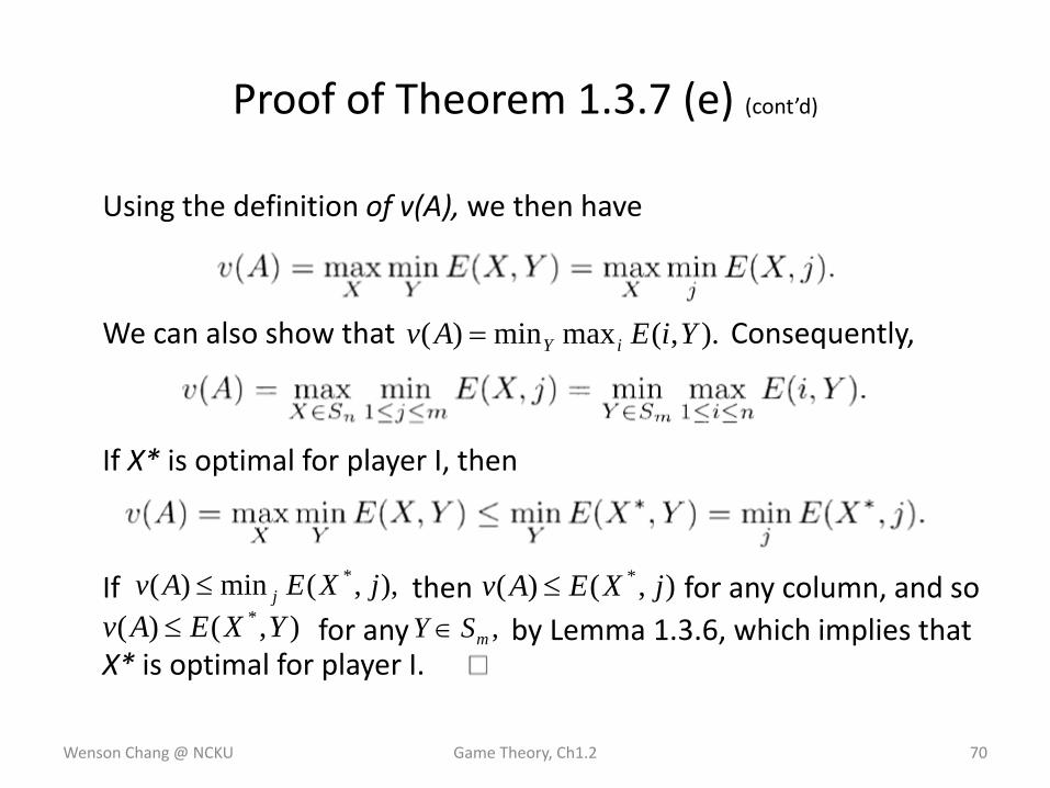
Using the definition of v(A), we then have
We can also show that Consequently,
If X* is optimal for player I, then
If then for any column, and sofor any by Lemma 1.3.6, which implies that
X* is optimal for player I.
Wenson Chang @ NCKU Game Theory, Ch1.2 70
Proof of Theorem 1.3.7 (e) (cont’d)
),,(min)( * jXEAv j≤
).,(maxmin)( YiEAv iY=
),()( * jXEAv ≤),()( * YXEAv ≤ ,mSY ∈
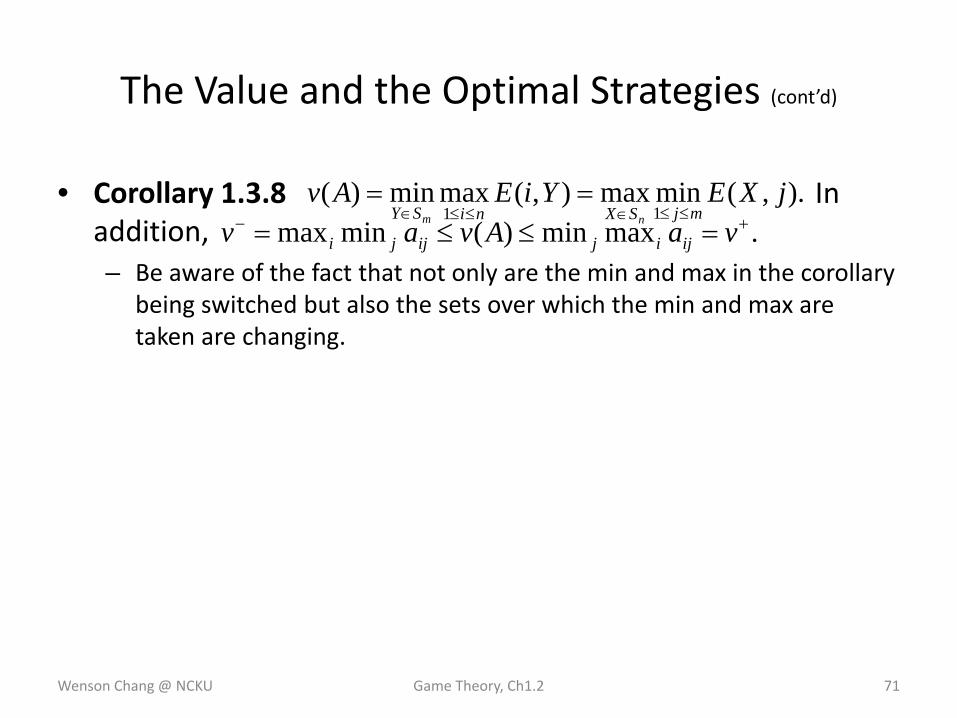
• Corollary 1.3.8 In addition,– Be aware of the fact that not only are the min and max in the corollary
being switched but also the sets over which the min and max are taken are changing.
Wenson Chang @ NCKU Game Theory, Ch1.2 71
The Value and the Optimal Strategies (cont’d)
).,(minmax),(maxmin)(11
jXEYiEAvmjSXniSY nm ≤≤∈≤≤∈
==.maxmin)(minmax +− =≤≤= vaAvav ijijijji
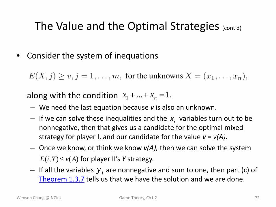
• Consider the system of inequations
along with the condition– We need the last equation because v is also an unknown.
– If we can solve these inequalities and the variables turn out to be nonnegative, then that gives us a candidate for the optimal mixed strategy for player I, and our candidate for the value v = v(A).
– Once we know, or think we know v(A), then we can solve the system
for player II’s Y strategy.
– If all the variables are nonnegative and sum to one, then part (c) of Theorem 1.3.7 tells us that we have the solution and we are done.
Wenson Chang @ NCKU Game Theory, Ch1.2 72
The Value and the Optimal Strategies (cont’d)
.1...1 =++ nxx
ix
)(),( AvYiE ≤
jy
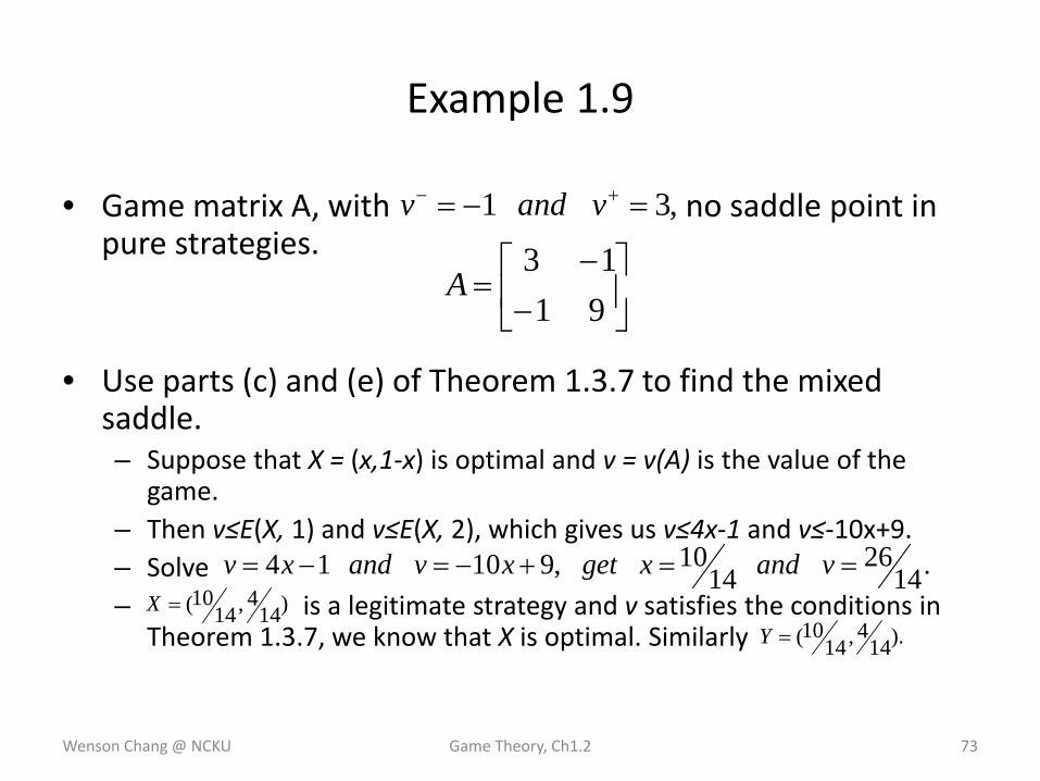
Example 1.9
• Game matrix A, with no saddle point in pure strategies.
• Use parts (c) and (e) of Theorem 1.3.7 to find the mixed saddle.– Suppose that X = (x,1‐x) is optimal and v = v(A) is the value of the
game.– Then v≤E(X, 1) and v≤E(X, 2), which gives us v≤4x‐1 and v≤‐10x+9.– Solve – is a legitimate strategy and v satisfies the conditions in
Theorem 1.3.7, we know that X is optimal. Similarly
Wenson Chang @ NCKU Game Theory, Ch1.2 73
⎥⎦
⎤⎢⎣
⎡−
−=
9113
A
,31 =−= +− vandv
)144,14
10(=X).14
4,1410(=Y
.1426
1410,91014 ==+−=−= vandxgetxvandxv
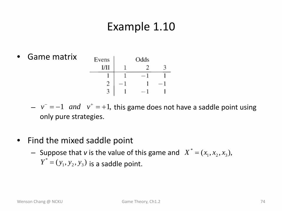
Example 1.10
• Game matrix
– this game does not have a saddle point using only pure strategies.
• Find the mixed saddle point– Suppose that v is the value of this game and
is a saddle point.
Wenson Chang @ NCKU Game Theory, Ch1.2 74
,11 +=−= +− vandv
),,,( 321* xxxX =
),,( 321* yyyY =
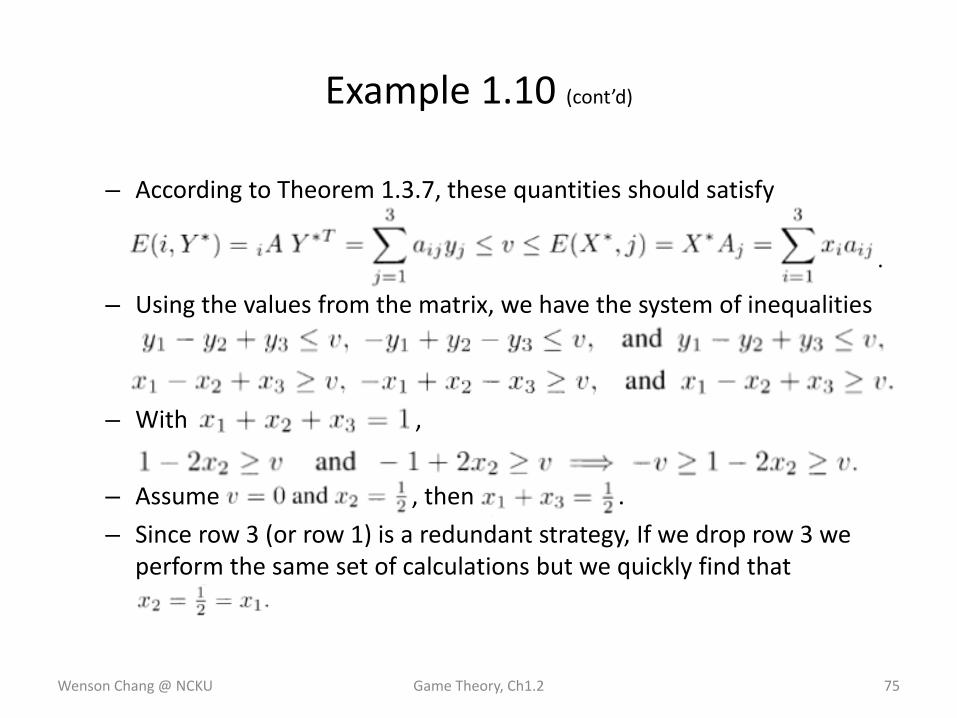
– According to Theorem 1.3.7, these quantities should satisfy
– Using the values from the matrix, we have the system of inequalities
– With ,
– Assume , then .
– Since row 3 (or row 1) is a redundant strategy, If we drop row 3 we perform the same set of calculations but we quickly find that
Wenson Chang @ NCKU Game Theory, Ch1.2 75
Example 1.10 (cont’d)
.
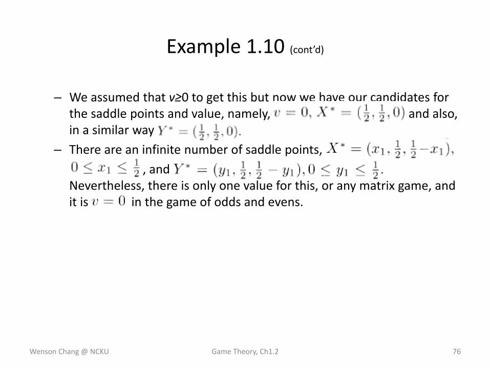
– We assumed that v≥0 to get this but now we have our candidates for the saddle points and value, namely, and also, in a similar way
– There are an infinite number of saddle points,
, and Nevertheless, there is only one value for this, or any matrix game, and it is in the game of odds and evens.
Wenson Chang @ NCKU Game Theory, Ch1.2 76
Example 1.10 (cont’d)
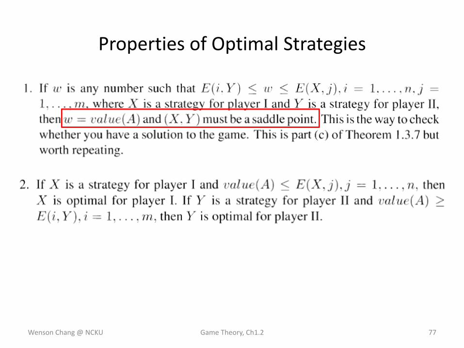
Properties of Optimal Strategies
Wenson Chang @ NCKU Game Theory, Ch1.2 77
Wenson Chang @ NCKU Game Theory, Ch1.2 78
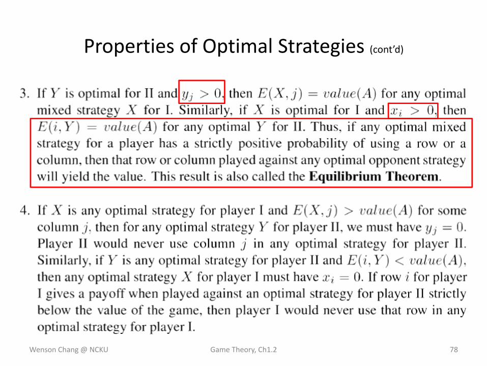
Properties of Optimal Strategies (cont’d)
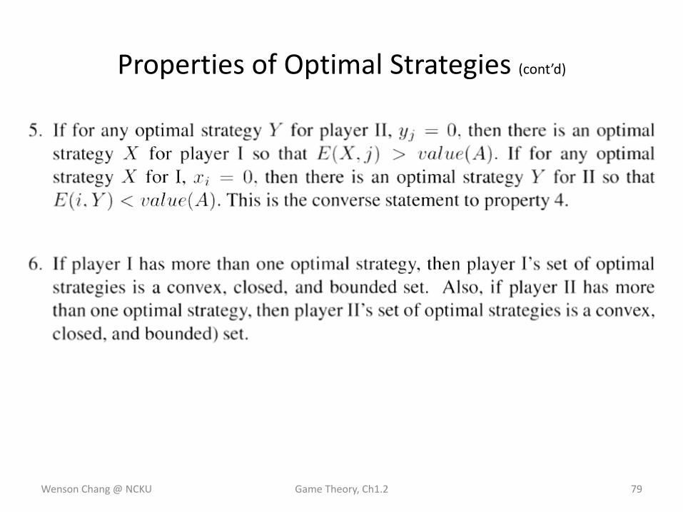
Wenson Chang @ NCKU Game Theory, Ch1.2 79
Properties of Optimal Strategies (cont’d)
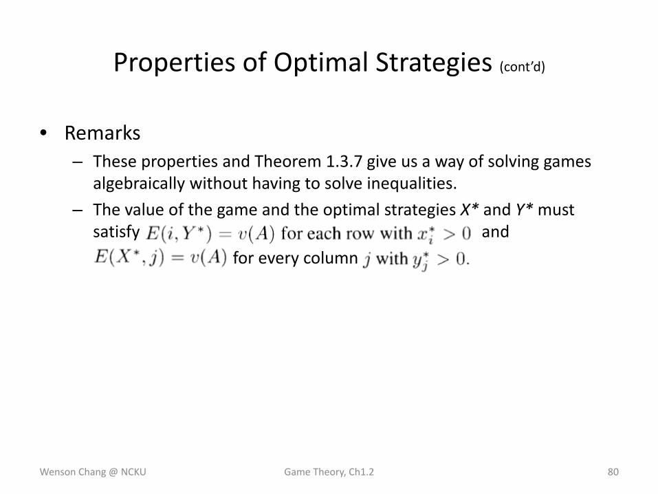
• Remarks– These properties and Theorem 1.3.7 give us a way of solving games
algebraically without having to solve inequalities.
– The value of the game and the optimal strategies X* and Y* must satisfy and
for every column
Wenson Chang @ NCKU Game Theory, Ch1.2 80
Properties of Optimal Strategies (cont’d)
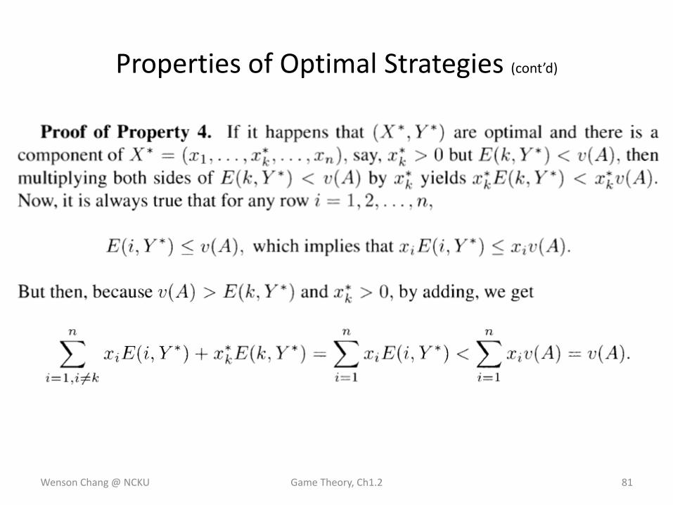
Wenson Chang @ NCKU Game Theory, Ch1.2 81
Properties of Optimal Strategies (cont’d)
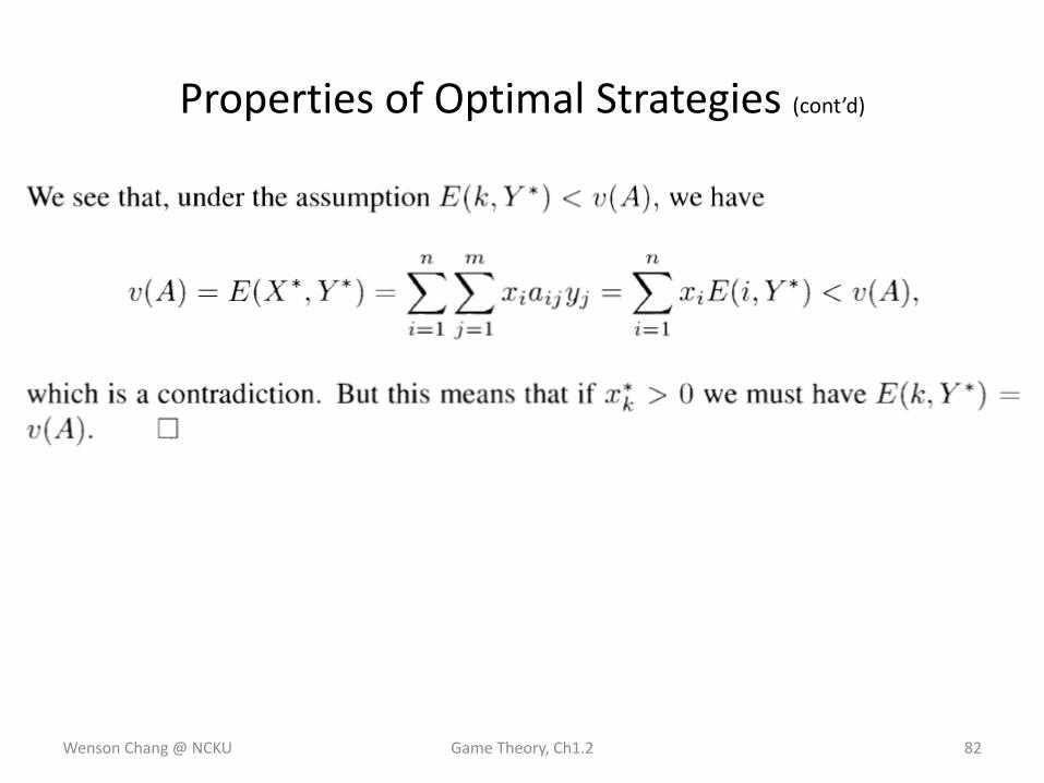
Wenson Chang @ NCKU Game Theory, Ch1.2 82
Properties of Optimal Strategies (cont’d)

• Consider the game matrix
– Conjecture
By property 3 for
Wenson Chang @ NCKU Game Theory, Ch1.2 83
Example 1.11
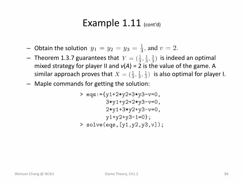
– Obtain the solution
– Theorem 1.3.7 guarantees that is indeed an optimal mixed strategy for player II and v(A) = 2 is the value of the game. A similar approach proves that is also optimal for player I.
– Maple commands for getting the solution:
Wenson Chang @ NCKU Game Theory, Ch1.2 84
Example 1.11 (cont’d)
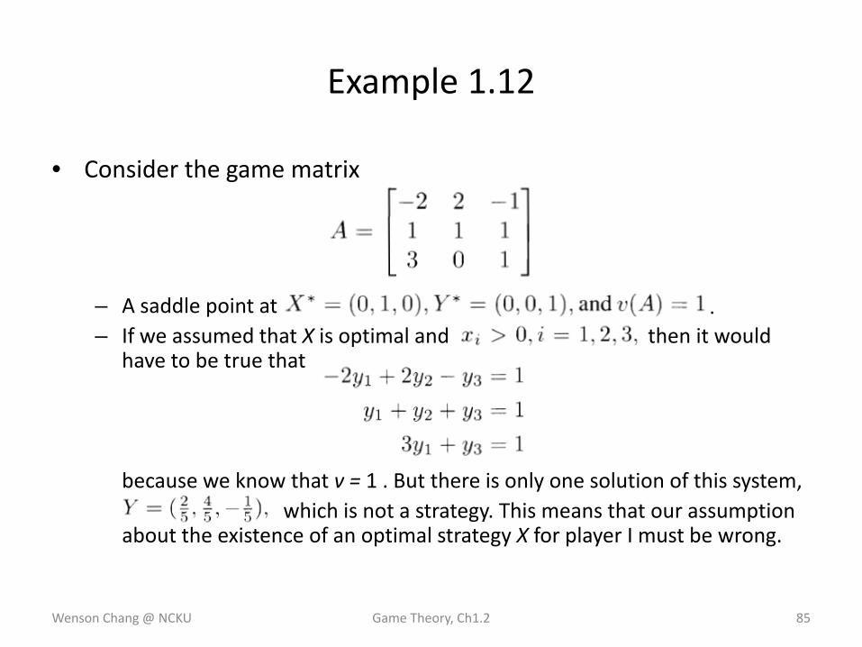
• Consider the game matrix
– A saddle point at .– If we assumed that X is optimal and then it would
have to be true that
because we know that v = 1 . But there is only one solution of this system, which is not a strategy. This means that our assumption
about the existence of an optimal strategy X for player I must be wrong.
Wenson Chang @ NCKU Game Theory, Ch1.2 85
Example 1.12
.
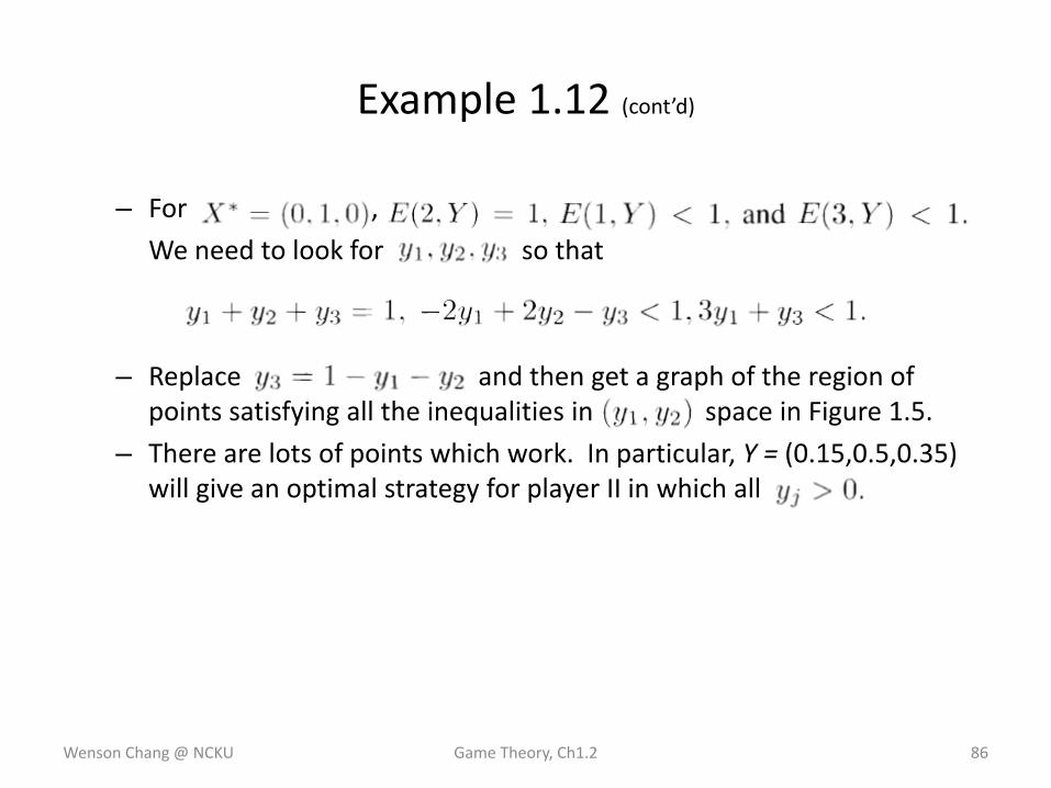
– For ,
We need to look for so that
– Replace and then get a graph of the region of points satisfying all the inequalities in space in Figure 1.5.
– There are lots of points which work. In particular, Y = (0.15,0.5,0.35) will give an optimal strategy for player II in which all
Wenson Chang @ NCKU Game Theory, Ch1.2 86
Example 1.12 (cont’d)
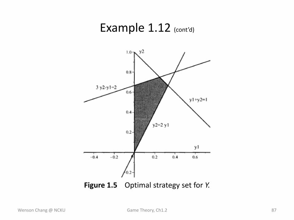
Figure 1.5 Optimal strategy set for Y.
Wenson Chang @ NCKU Game Theory, Ch1.2 87
Example 1.12 (cont’d)
Dominated Strategies
• Sometimes we can reduce the size of the matrix A by eliminating rows or columns (i.e., strategies) that will never be used because there is always a better row or column to use. This is elimination by dominance.– If we can reduce it to a 2 x m or n x 2 game, we can solve it by a
graphical procedure. If we can reduce it to a 2 x 2 matrix, we can use the formulas (following on).
Wenson Chang @ NCKU Game Theory, Ch1.2 88
• Definition 1.3.9 Row i dominates row k if for all
This allows us to remove row k. Column j dominates column k if This allows us to remove column k. Strict dominance means the inequalities are strict in at least one payoff pair in a row or a column.
• Remark. A row that is dropped because it is strictly dominated is played in a mixed strategy with probability 0. But a row that is dropped because it is equal to another row may not have probability 0 of being played.
Wenson Chang @ NCKU Game Theory, Ch1.2 89
Dominated Strategies (cont’d)
– For example, suppose that we have a matrix with three rows and row 2 is the same as row 3. If we drop row 3, we now have two rows and the resulting optimal strategy will look like .
– For the original game the optimal strategy could be or
or in fact for any
and this is the most general description.
– A duplicate row is a redundant row and may be dropped to reduce the size of the matrix. But you must account for redundant strategies.
Wenson Chang @ NCKU Game Theory, Ch1.2 90
Dominated Strategies (cont’d)
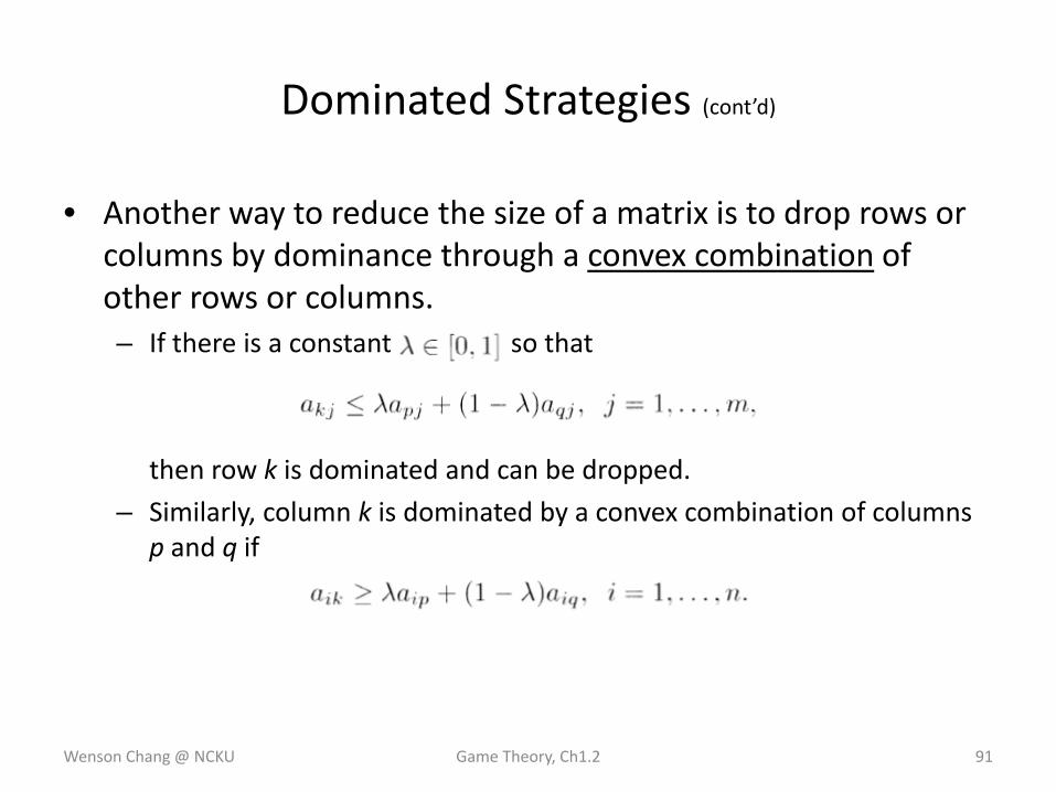
• Another way to reduce the size of a matrix is to drop rows or columns by dominance through a convex combination of other rows or columns. – If there is a constant so that
then row k is dominated and can be dropped.
– Similarly, column k is dominated by a convex combination of columns p and q if
Wenson Chang @ NCKU Game Theory, Ch1.2 91
Dominated Strategies (cont’d)
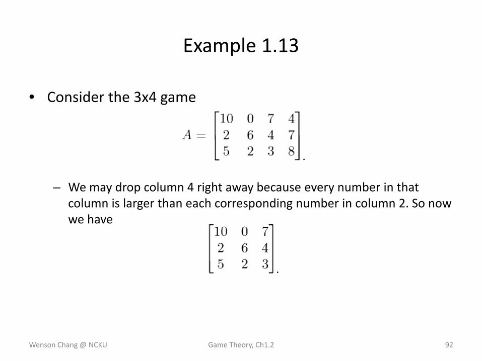
• Consider the 3x4 game
– We may drop column 4 right away because every number in that column is larger than each corresponding number in column 2. So now we have
Wenson Chang @ NCKU Game Theory, Ch1.2 92
Example 1.13
.
.
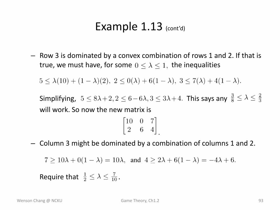
– Row 3 is dominated by a convex combination of rows 1 and 2. If that is true, we must have, for some 0 < the inequalities
Simplifying, This says any
will work. So now the new matrix is
– Column 3 might be dominated by a combination of columns 1 and 2.
Require that .
Wenson Chang @ NCKU Game Theory, Ch1.2 93
Example 1.13 (cont’d)
.
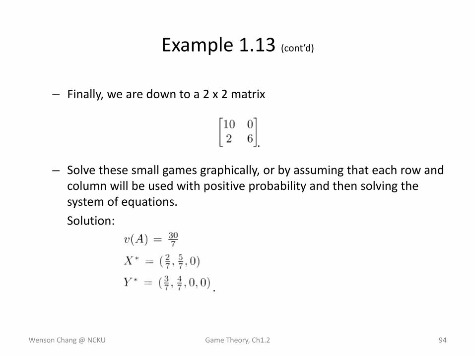
– Finally, we are down to a 2 x 2 matrix
– Solve these small games graphically, or by assuming that each row and column will be used with positive probability and then solving the system of equations.
Solution:
Wenson Chang @ NCKU Game Theory, Ch1.2 94
Example 1.13 (cont’d)
.
.
Solving 2 × 2 Games Graphically
Wenson Chang @ NCKU Game Theory, Ch1.2 95
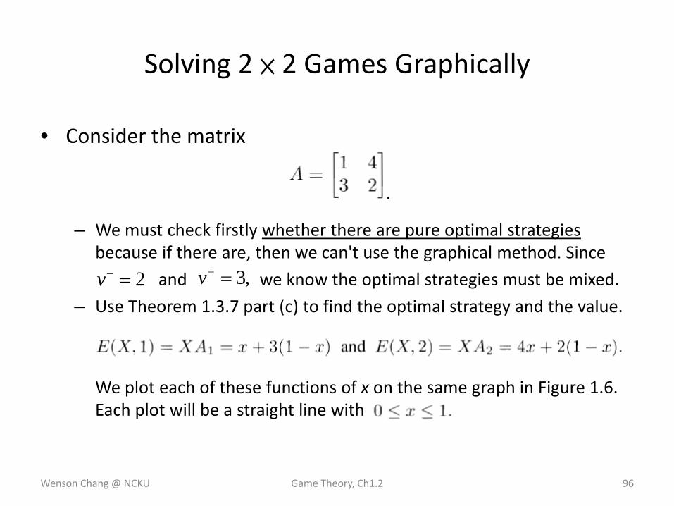
Solving 2 × 2 Games Graphically
• Consider the matrix
– We must check firstly whether there are pure optimal strategiesbecause if there are, then we can't use the graphical method. Since
and we know the optimal strategies must be mixed.
– Use Theorem 1.3.7 part (c) to find the optimal strategy and the value.
We plot each of these functions of x on the same graph in Figure 1.6. Each plot will be a straight line with
Wenson Chang @ NCKU Game Theory, Ch1.2 96
2=−v ,3=+v
.
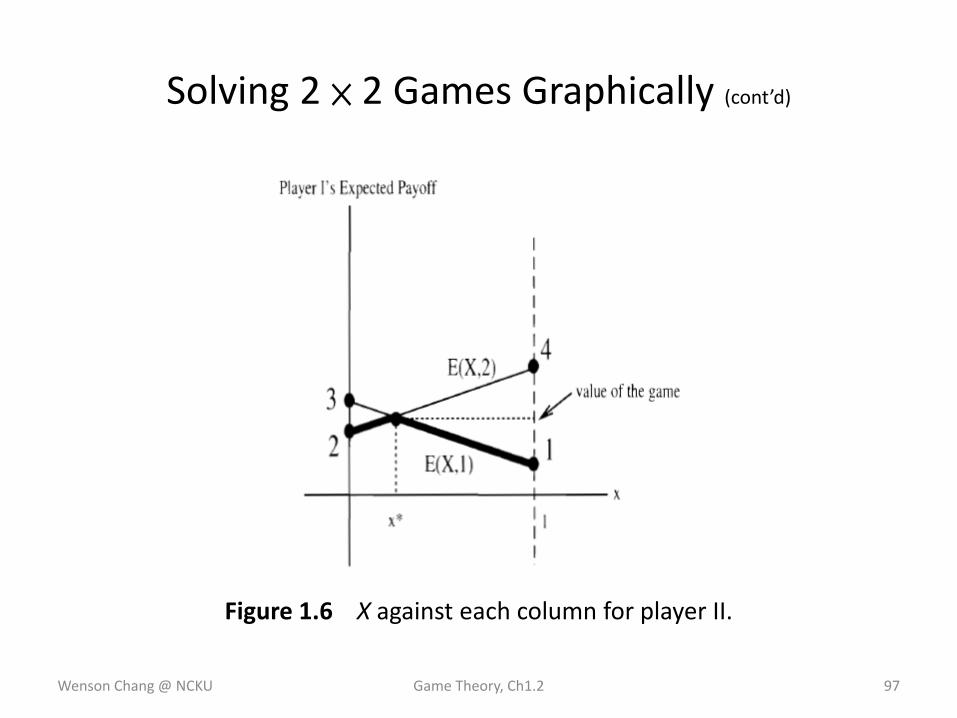
Figure 1.6 X against each column for player II.
Wenson Chang @ NCKU Game Theory, Ch1.2 97
Solving 2 × 2 Games Graphically (cont’d)
• Analysis– The point at which the two lines intersect is
– If player I chooses an then the best I can receive is on the highest line when is on the left of .
•• Player I will receive this higher payoff only if player II decides to play column 1.
• If player II use column 2, then I would receive a payoff on the lower line
– If player I chooses an •• The best I could get would happen if player II chose to use column 2.
• If player II use column 1, then I would receives some payoff on the line
Wenson Chang @ NCKU Game Theory, Ch1.2 98
Analysis of the Graph
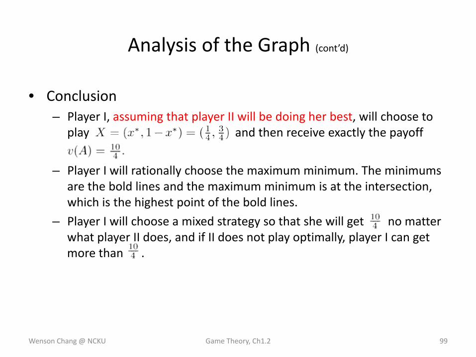
• Conclusion– Player I, assuming that player II will be doing her best, will choose to
play and then receive exactly the payoff
– Player I will rationally choose the maximum minimum. The minimums are the bold lines and the maximum minimum is at the intersection, which is the highest point of the bold lines.
– Player I will choose a mixed strategy so that she will get no matter what player II does, and if II does not play optimally, player I can get more than .
Wenson Chang @ NCKU Game Theory, Ch1.2 99
Analysis of the Graph (cont’d)
Graphical Solution of 2 ×mand n × 2 Games
Wenson Chang @ NCKU Game Theory, Ch1.2 100
Graphical Solution of 2 ×m Games
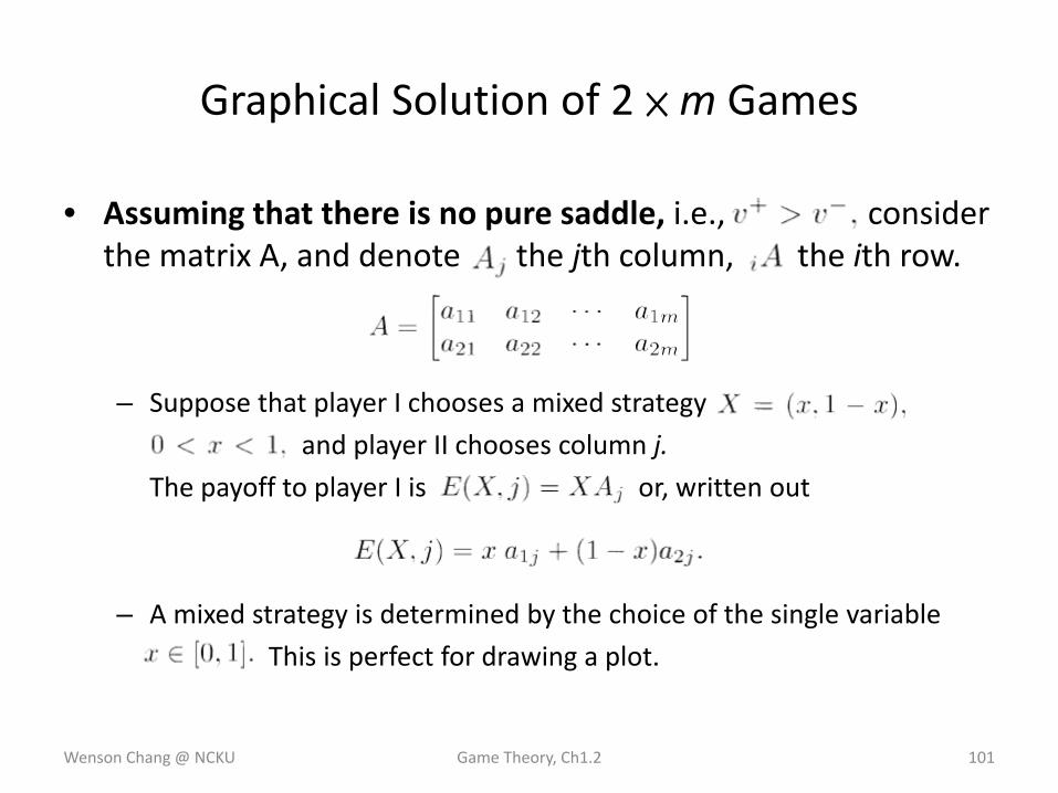
• Assuming that there is no pure saddle, i.e., consider the matrix A, and denote the jth column, the ith row.
– Suppose that player I chooses a mixed strategy
and player II chooses column j.
The payoff to player I is or, written out
– A mixed strategy is determined by the choice of the single variable
This is perfect for drawing a plot.
Wenson Chang @ NCKU Game Theory, Ch1.2 101
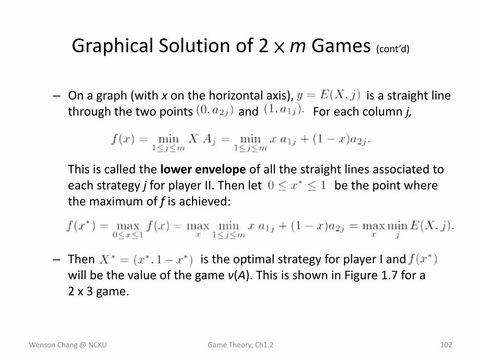
– On a graph (with x on the horizontal axis), is a straight line through the two points and For each column j,
This is called the lower envelope of all the straight lines associated to each strategy j for player II. Then let be the point where the maximum of f is achieved:
– Then is the optimal strategy for player I and will be the value of the game v(A). This is shown in Figure 1.7 for a 2 x 3 game.
Wenson Chang @ NCKU Game Theory, Ch1.2 102
Graphical Solution of 2 ×m Games (cont’d)
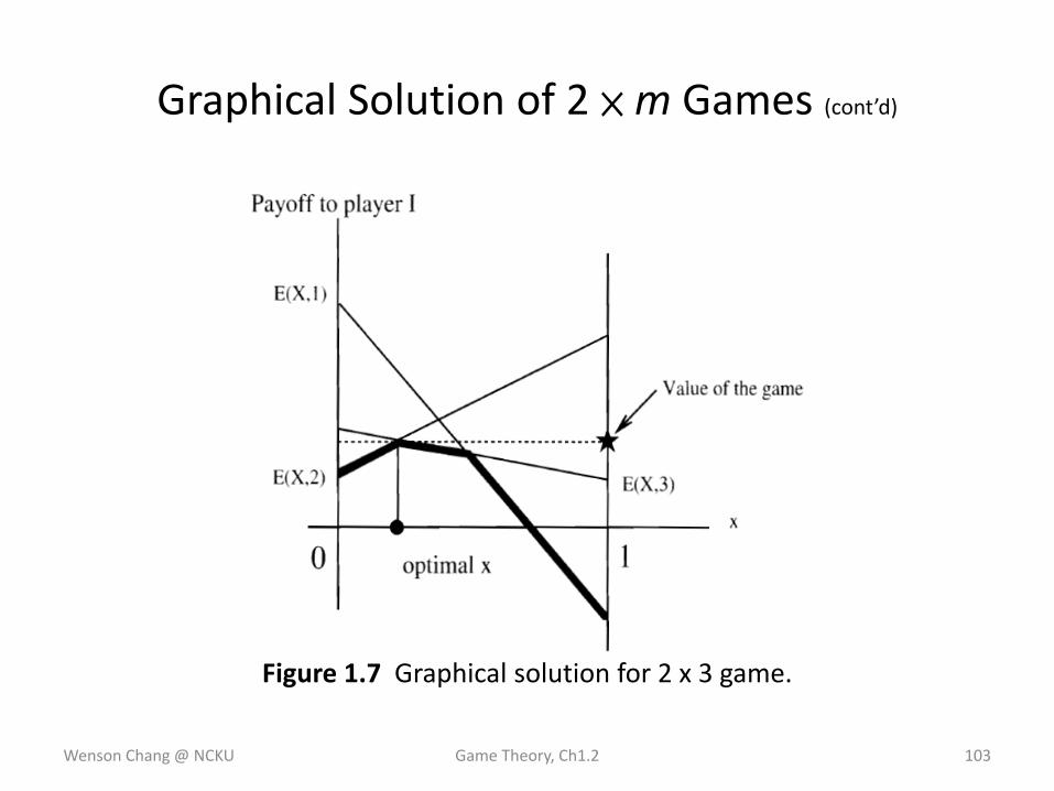
Figure 1.7 Graphical solution for 2 x 3 game.
Wenson Chang @ NCKU Game Theory, Ch1.2 103
Graphical Solution of 2 ×m Games (cont’d)
– Each line represents the payoff that player I would receive by playing the mixed strategy with player II always playing a fixed column.
• If player I decides to play the mixed strategy where is to the left of the optimal value, then player II would choose to play column 2.
• If player I decides to play the mixed strategy where is to the right of the optimal value, then player II would choose to play column 3, up to the point of intersection where and then switch to column 1.
• Player I would choose the x that guarantees that she will receive the maximum of all the lower points of the lines.
Wenson Chang @ NCKU Game Theory, Ch1.2 104
Graphical Solution of 2 ×m Games (cont’d)
– By choosing this optimal value, say, x*, it will be the case that player II would play some combination of columns 2 and 3.
• It would be a mixture (a convex combination) of the columns because if player II always chose to play, say, column 2, then player I could do better by changing her mixed strategy to a point to the right of the optimal value.
– For finding the optimal strategy for player II, the only two columns being used in an optimal strategy for player I are columns 2 and 3.
• By the properties of optimal strategies (1.3.1), that for this particular graph we can eliminate column 1 and reduce to a 2 x 2 matrix.
Wenson Chang @ NCKU Game Theory, Ch1.2 105
Graphical Solution of 2 ×m Games (cont’d)
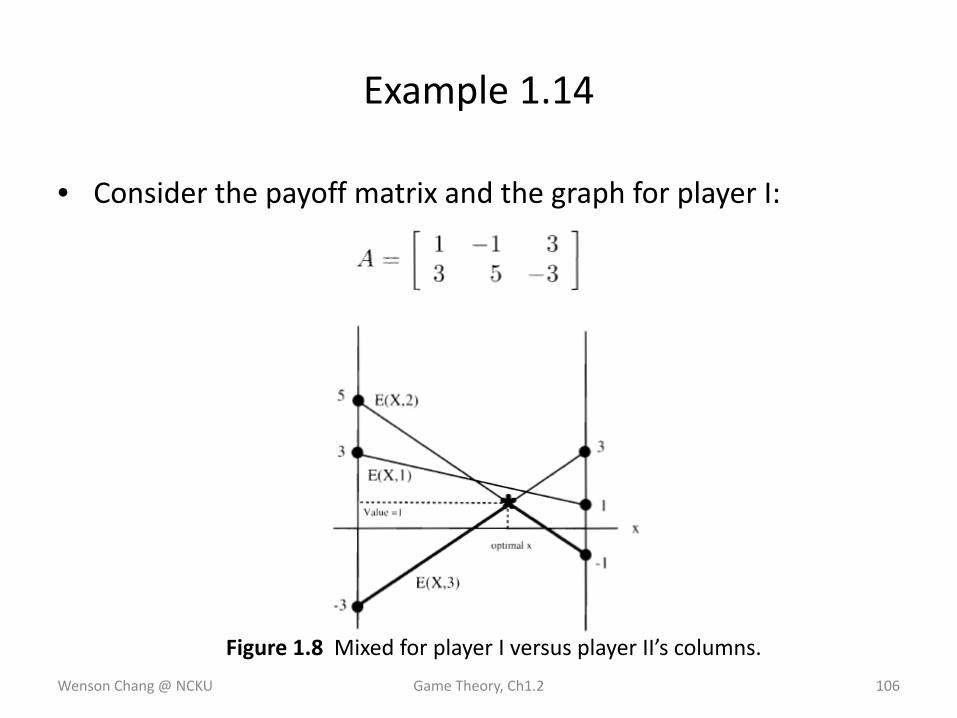
Example 1.14
• Consider the payoff matrix and the graph for player I:
Wenson Chang @ NCKU Game Theory, Ch1.2 106
Figure 1.8 Mixed for player I versus player II’s columns.
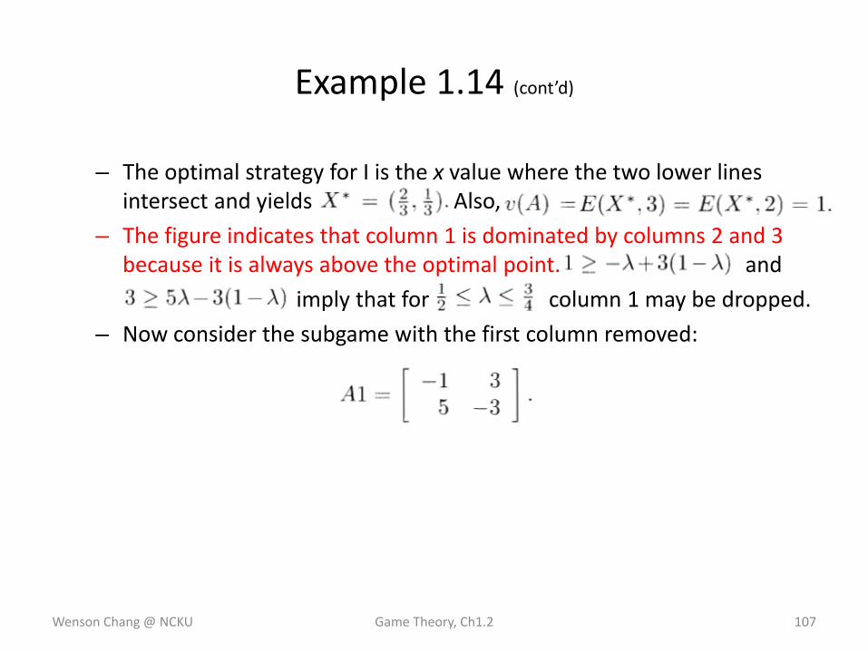
– The optimal strategy for I is the x value where the two lower lines intersect and yields Also,
– The figure indicates that column 1 is dominated by columns 2 and 3 because it is always above the optimal point. and
imply that for column 1 may be dropped.
– Now consider the subgame with the first column removed:
Wenson Chang @ NCKU Game Theory, Ch1.2 107
Example 1.14 (cont’d)
– Solve this graphically for player II assuming that II uses Consider the payoffs .
– Player II wants to choose y so that no matter what I does she is guaranteed the smallest maximum. This is now the lowest point of the highest part of the lines in Figure 1.9.
– The lines intersect with
– The optimal strategy for II is , and the value
Wenson Chang @ NCKU Game Theory, Ch1.2 108
Example 1.14 (cont’d)
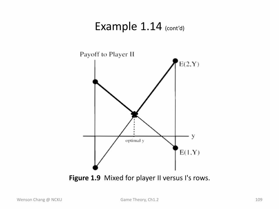
Figure 1.9 Mixed for player II versus I's rows.
Wenson Chang @ NCKU Game Theory, Ch1.2 109
Example 1.14 (cont’d)
Graphical Solution of n × 2 Games
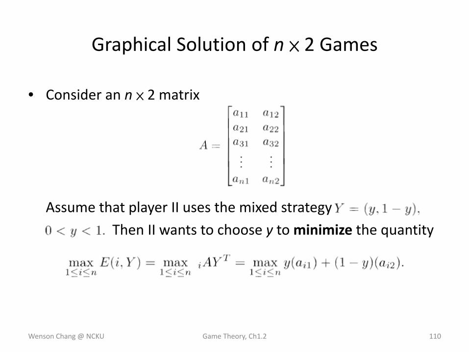
• Consider an n × 2 matrix
Assume that player II uses the mixed strategy
Then II wants to choose y to minimize the quantity
Wenson Chang @ NCKU Game Theory, Ch1.2 110
– The graph of the payoffs (to player I) will be a straight line.
– Player I will want to go as high as possible; Player II will play the mixed strategy which will give the lowest maximum.
– The optimal will be the point giving the minimum of the upper envelope.
Wenson Chang @ NCKU Game Theory, Ch1.2 111
Graphical Solution of n × 2 Games (cont’d)
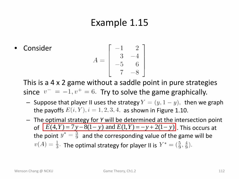
• Consider
This is a 4 x 2 game without a saddle point in pure strategies since Try to solve the game graphically.– Suppose that player II uses the strategy then we graph
the payoffs as shown in Figure 1.10.
– The optimal strategy for Y will be determined at the intersection point of . This occurs at the point and the corresponding value of the game will be
The optimal strategy for player II is
Wenson Chang @ NCKU Game Theory, Ch1.2 112
Example 1.15
(4, ) 7 8(1 ) and (1, ) 2(1 )E Y y y E Y y y= − − = − + −
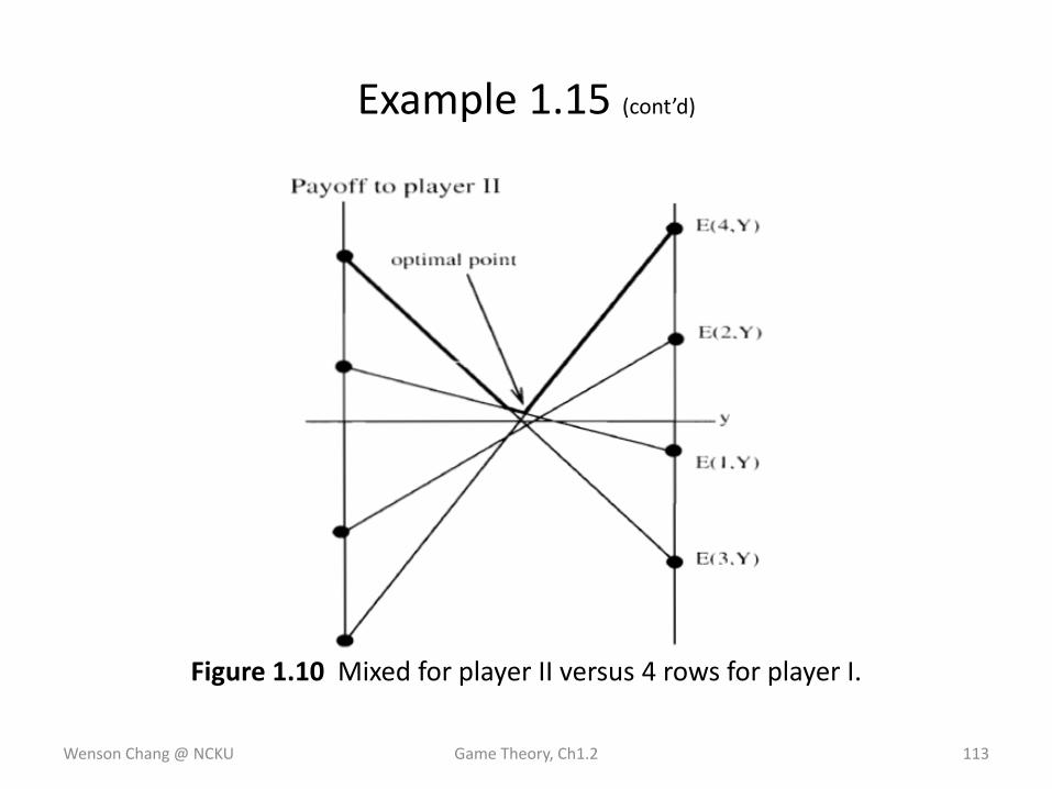
Figure 1.10 Mixed for player II versus 4 rows for player I.
Wenson Chang @ NCKU Game Theory, Ch1.2 113
Example 1.15 (cont’d)
– Since and row 2 is dominated by a convex combination of rows 1 and 4; so row 2 may be dropped.
– Row 3 is dropped because its payoff line does not pass through the optimal point.
– Considering the matrix using only rows 1 and 4, we now calculate
which intersect at
– We obtain that row 1 should be used with probability and row 4 should be used with probability
– In the above, we drop rows 2 and 3 to find the optimal strategy for player 1. In general, we may drop the rows ( or columns) not used to get the optimal intersection point. This is not always true !
Wenson Chang @ NCKU Game Theory, Ch1.2 114
Example 1.15 (cont’d)
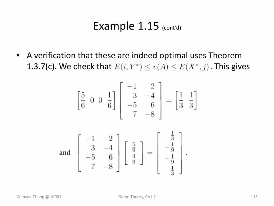
• A verification that these are indeed optimal uses Theorem 1.3.7(c). We check that . This gives
Wenson Chang @ NCKU Game Theory, Ch1.2 115
Example 1.15 (cont’d)
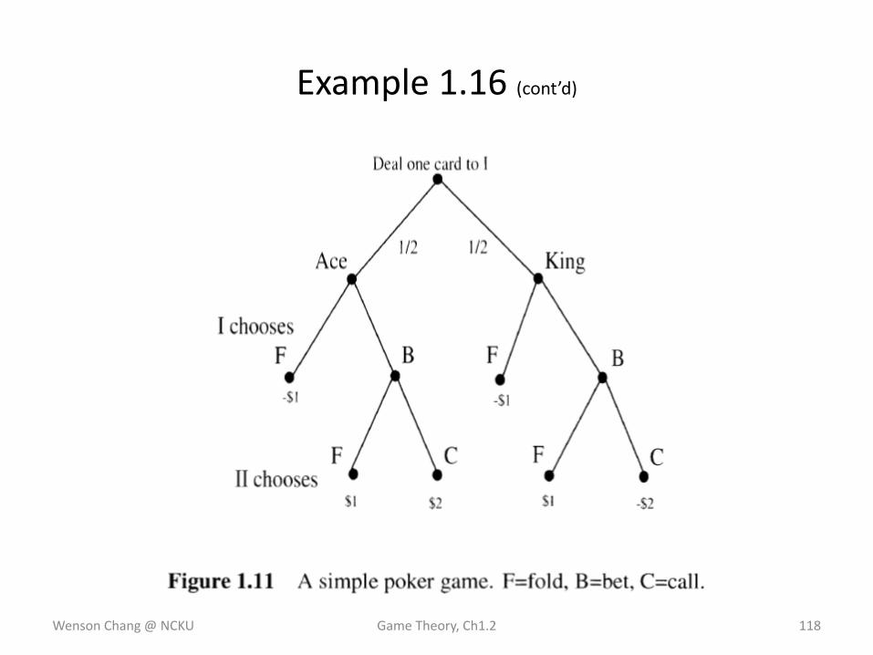
• Poker game rules– Player I is dealt a card that may be an ace or a king. Player I sees the
result but II does not. Player I may then choose to fold or bet.
– If I folds, he has to pay player II $1. If I bets, player II may choose to fold or call.
– If II folds, she pays player I $1. If player II calls and the card is a king, then player I pays player II $2, but if the card comes up ace, then player II pays player I $2.
– I must pay II $1 when I gets a king and he folds.
– Player I is hoping that player II will fold if I bets while holding a king. This is the element of bluffing, because if II calls while I is holding a king, then I must pay II $2.
Wenson Chang @ NCKU Game Theory, Ch1.2 116
Example 1.16
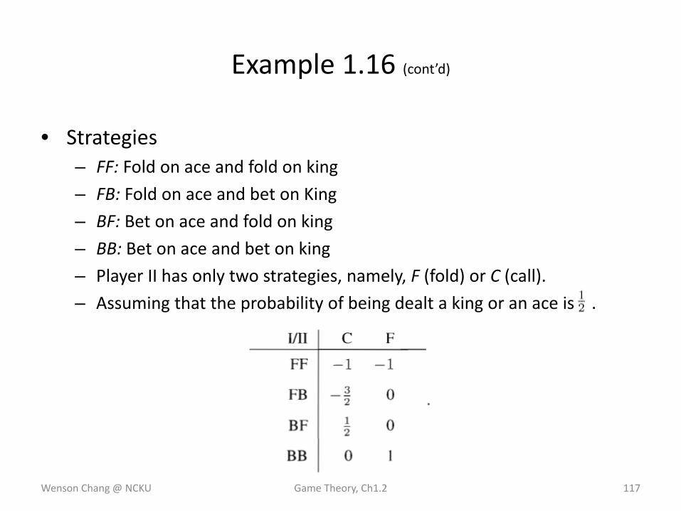
• Strategies– FF: Fold on ace and fold on king
– FB: Fold on ace and bet on King
– BF: Bet on ace and fold on king
– BB: Bet on ace and bet on king
– Player II has only two strategies, namely, F (fold) or C (call).
– Assuming that the probability of being dealt a king or an ace is .
Wenson Chang @ NCKU Game Theory, Ch1.2 117
Example 1.16 (cont’d)
Wenson Chang @ NCKU Game Theory, Ch1.2 118
Example 1.16 (cont’d)
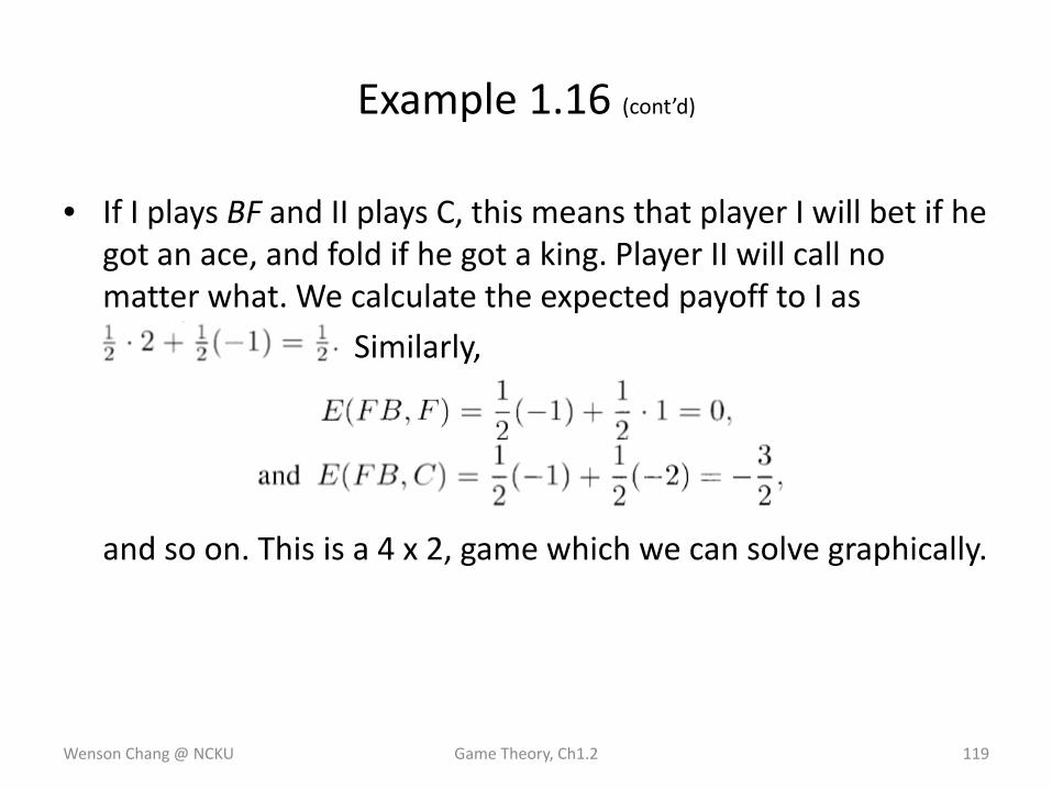
• If I plays BF and II plays C, this means that player I will bet if he got an ace, and fold if he got a king. Player II will call no matter what. We calculate the expected payoff to I as
Similarly,
and so on. This is a 4 x 2, game which we can solve graphically.
Wenson Chang @ NCKU Game Theory, Ch1.2 119
Example 1.16 (cont’d)
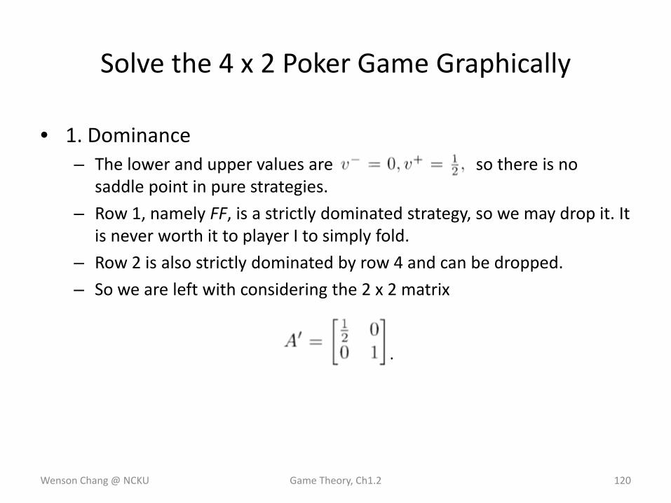
• 1. Dominance– The lower and upper values are so there is no
saddle point in pure strategies.
– Row 1, namely FF, is a strictly dominated strategy, so we may drop it. It is never worth it to player I to simply fold.
– Row 2 is also strictly dominated by row 4 and can be dropped.
– So we are left with considering the 2 x 2 matrix
Wenson Chang @ NCKU Game Theory, Ch1.2 120
Solve the 4 x 2 Poker Game Graphically
.
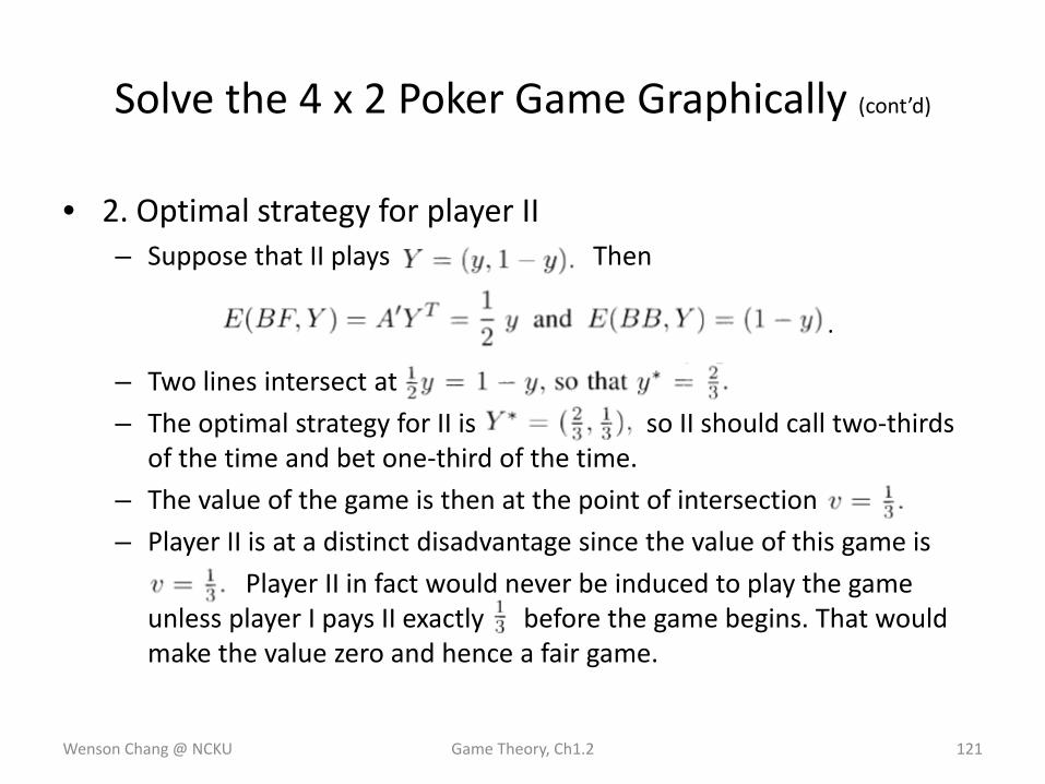
• 2. Optimal strategy for player II– Suppose that II plays Then
– Two lines intersect at
– The optimal strategy for II is so II should call two‐thirds of the time and bet one‐third of the time.
– The value of the game is then at the point of intersection
– Player II is at a distinct disadvantage since the value of this game is
Player II in fact would never be induced to play the game unless player I pays II exactly before the game begins. That would make the value zero and hence a fair game.
Wenson Chang @ NCKU Game Theory, Ch1.2 121
Solve the 4 x 2 Poker Game Graphically (cont’d)
.
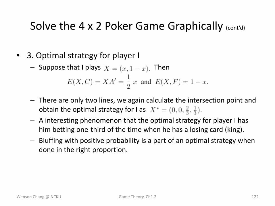
• 3. Optimal strategy for player I– Suppose that I plays Then
– There are only two lines, we again calculate the intersection point and obtain the optimal strategy for I as
– A interesting phenomenon that the optimal strategy for player I has him betting one‐third of the time when he has a losing card (king).
– Bluffing with positive probability is a part of an optimal strategy when done in the right proportion.
Wenson Chang @ NCKU Game Theory, Ch1.2 122
Solve the 4 x 2 Poker Game Graphically (cont’d)
Solve the 4 x 2 Poker Game Graphically (cont’d)
• Player II in fact would never be induced to play the game unless player I pays II exactly 1/3 before the game begins. – That would make the value zero and hence a fair game.
Wenson Chang @ NCKU Game Theory, Ch1.2 123
Best Response Strategies
Wenson Chang @ NCKU Game Theory, Ch1.2 124
Definition of Best Response Strategy
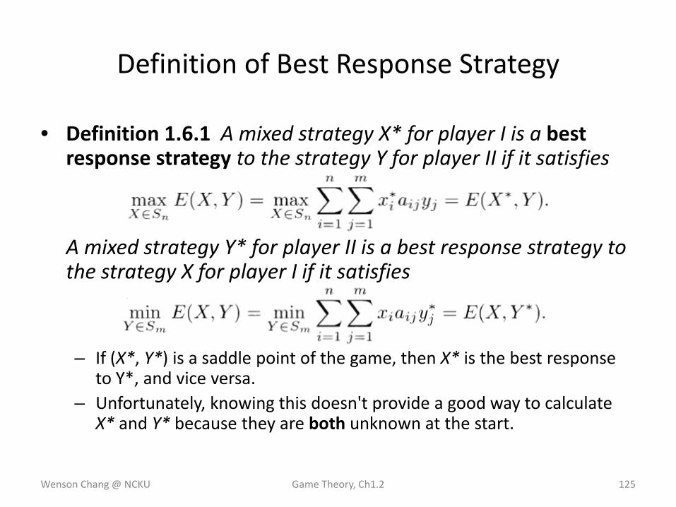
• Definition 1.6.1 A mixed strategy X* for player I is a best response strategy to the strategy Y for player II if it satisfies
A mixed strategy Y* for player II is a best response strategy to the strategy X for player I if it satisfies
– If (X*, Y*) is a saddle point of the game, then X* is the best response to Y*, and vice versa.
– Unfortunately, knowing this doesn't provide a good way to calculate X* and Y* because they are both unknown at the start.
Wenson Chang @ NCKU Game Theory, Ch1.2 125
Example 1.17
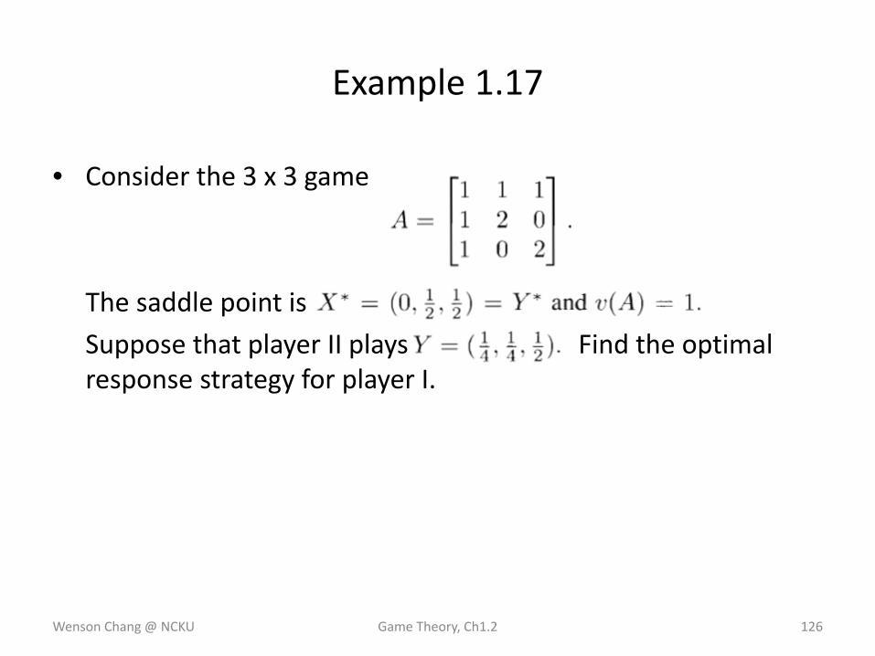
• Consider the 3 x 3 game
The saddle point is
Suppose that player II plays Find the optimal response strategy for player I.
Wenson Chang @ NCKU Game Theory, Ch1.2 126
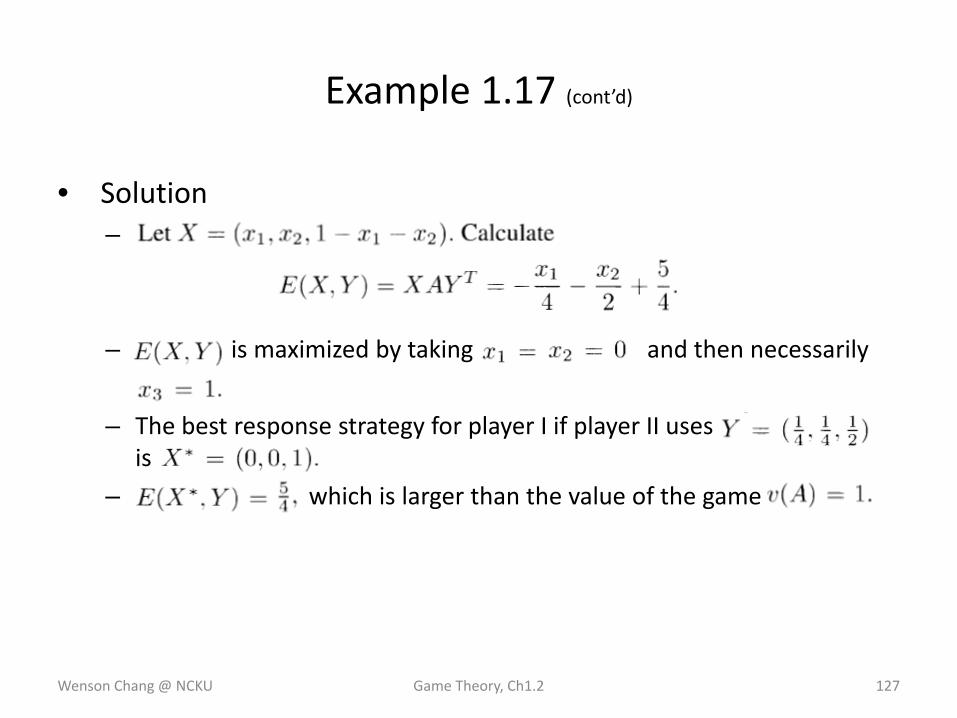
Example 1.17 (cont’d)
• Solution–
– is maximized by taking and then necessarily
– The best response strategy for player I if player II uses is
– which is larger than the value of the game
Wenson Chang @ NCKU Game Theory, Ch1.2 127

– How player 1 should play if player II decides to deviate from the optimal Y.
– This shows that any deviation from a saddle could result in a better payoff for the opposing player.
– If one player knows that the other player will not use her part of the saddle, then the best response may not be the strategy used in the saddle.
– In other words, if is a saddle point, the best response to
may not be but some other even though it will be the case that
Wenson Chang @ NCKU Game Theory, Ch1.2 128
Example 1.17 (cont’d)
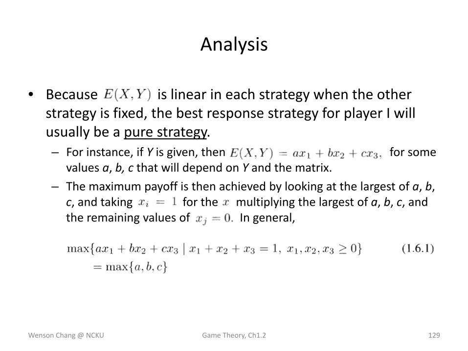
• Because is linear in each strategy when the other strategy is fixed, the best response strategy for player I will usually be a pure strategy.– For instance, if Y is given, then for some
values a, b, c that will depend on Y and the matrix.
– The maximum payoff is then achieved by looking at the largest of a, b,c, and taking for the multiplying the largest of a, b, c, and the remaining values of In general,
Wenson Chang @ NCKU Game Theory, Ch1.2 129
Analysis
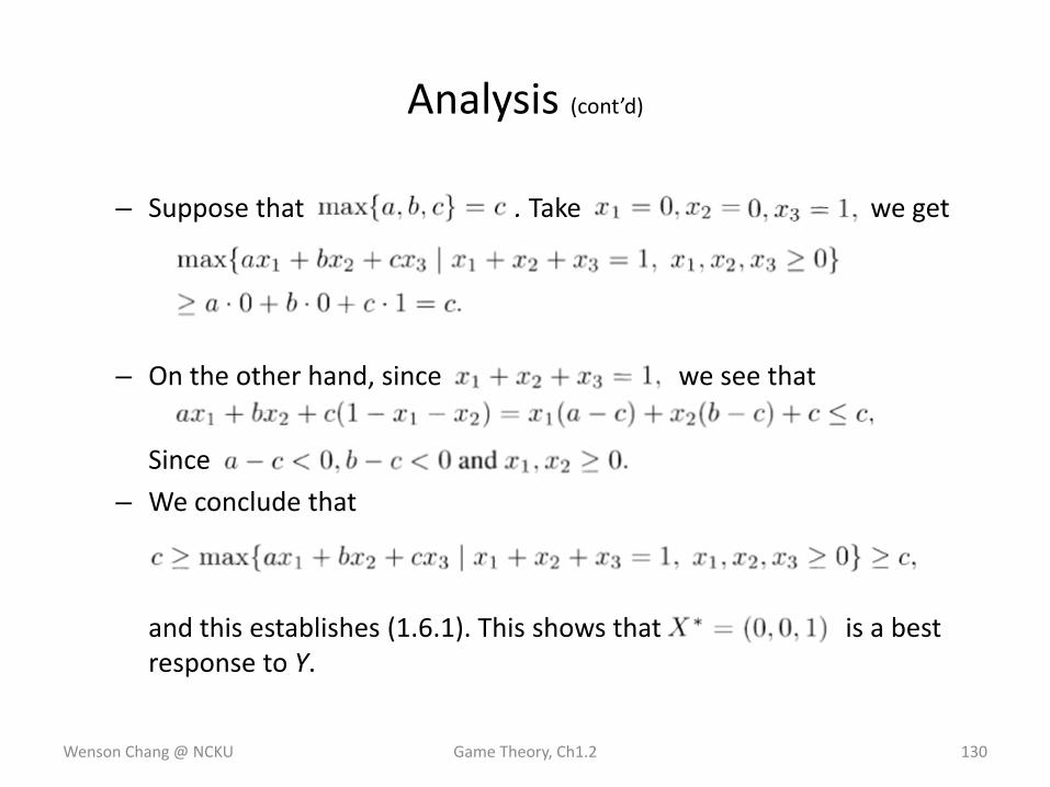
– Suppose that . Take we get
– On the other hand, since we see that
Since
– We conclude that
and this establishes (1.6.1). This shows that is a best response to Y.
Wenson Chang @ NCKU Game Theory, Ch1.2 130
Analysis (cont’d)
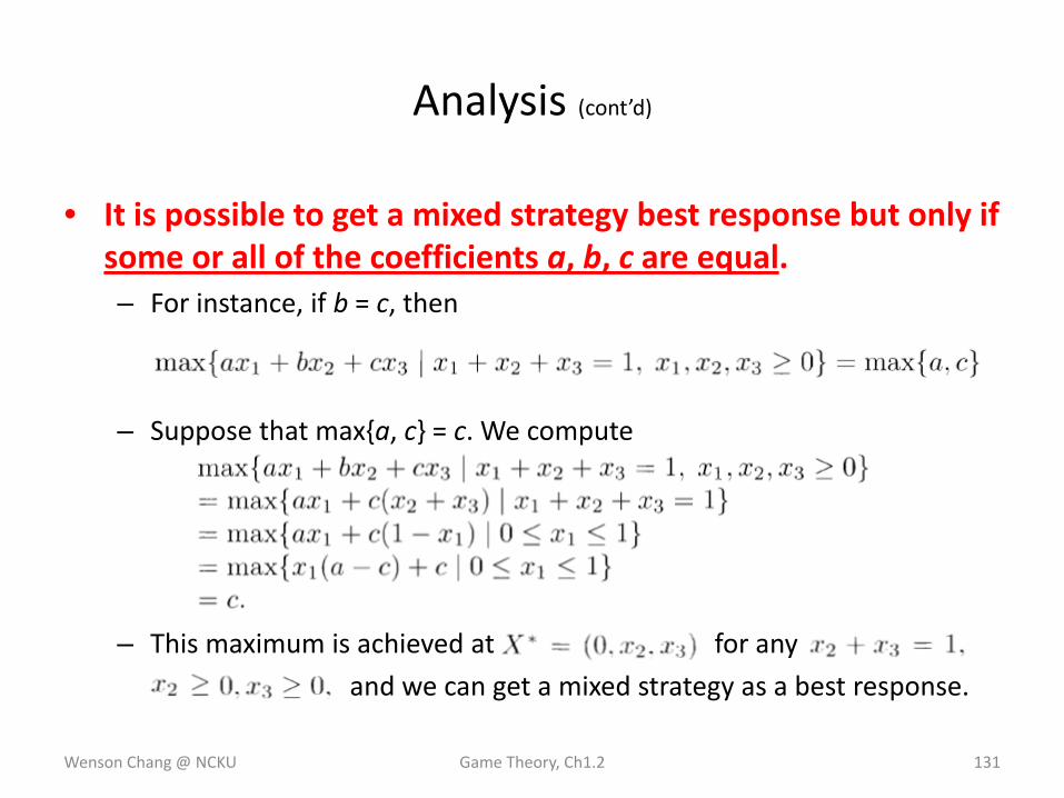
• It is possible to get a mixed strategy best response but only if some or all of the coefficients a, b, c are equal.– For instance, if b = c, then
– Suppose that max{a, c} = c. We compute
– This maximum is achieved at for any
and we can get a mixed strategy as a best response.
Wenson Chang @ NCKU Game Theory, Ch1.2 131
Analysis (cont’d)
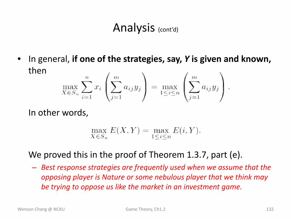
• In general, if one of the strategies, say, Y is given and known, then
In other words,
We proved this in the proof of Theorem 1.3.7, part (e).– Best response strategies are frequently used when we assume that the
opposing player is Nature or some nebulous player that we think may be trying to oppose us like the market in an investment game.
Wenson Chang @ NCKU Game Theory, Ch1.2 132
Analysis (cont’d)
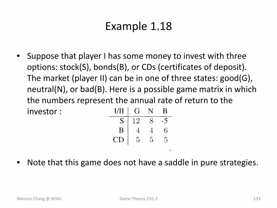
Example 1.18
• Suppose that player I has some money to invest with three options: stock(S), bonds(B), or CDs (certificates of deposit). The market (player II) can be in one of three states: good(G), neutral(N), or bad(B). Here is a possible game matrix in which the numbers represent the annual rate of return to the investor :
• Note that this game does not have a saddle in pure strategies.
Wenson Chang @ NCKU Game Theory, Ch1.2 133
.
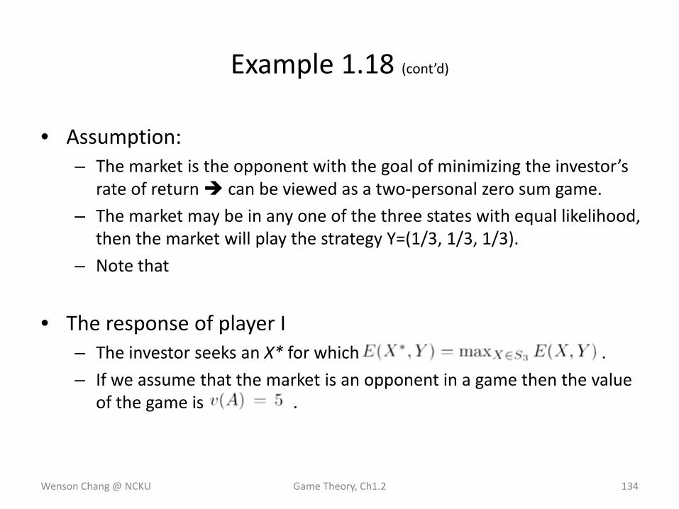
Example 1.18 (cont’d)
• Assumption: – The market is the opponent with the goal of minimizing the investor’s
rate of return can be viewed as a two‐personal zero sum game.– The market may be in any one of the three states with equal likelihood,
then the market will play the strategy Y=(1/3, 1/3, 1/3).
– Note that
• The response of player I– The investor seeks an X* for which .
– If we assume that the market is an opponent in a game then the value of the game is .
Wenson Chang @ NCKU Game Theory, Ch1.2 134
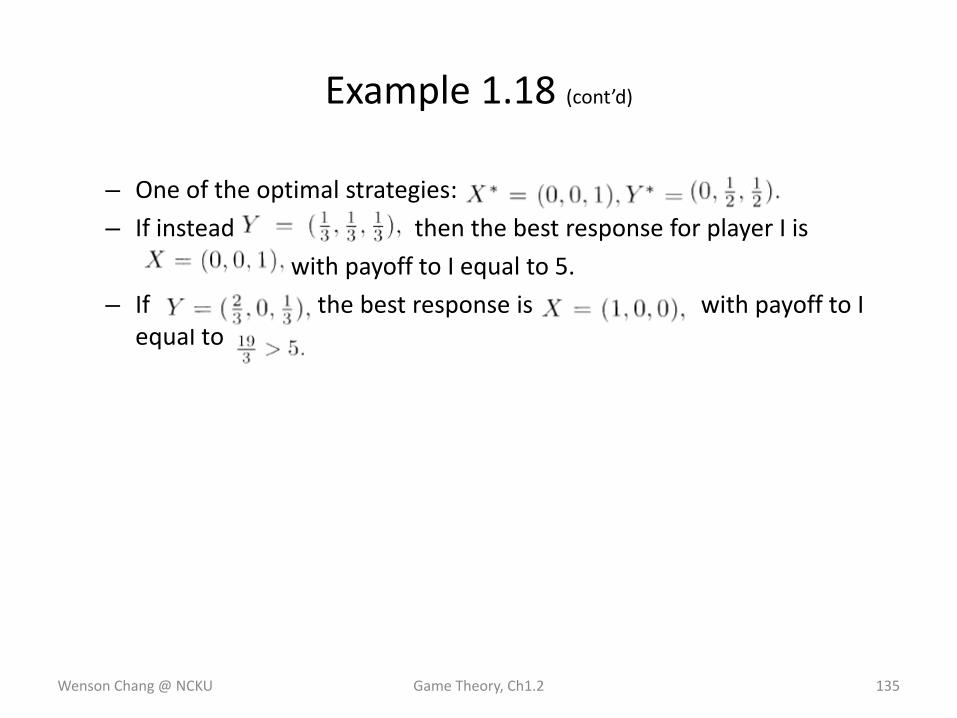
Example 1.18 (cont’d)
– One of the optimal strategies:
– If instead then the best response for player I is
with payoff to I equal to 5.
– If the best response is with payoff to I equal to
Wenson Chang @ NCKU Game Theory, Ch1.2 135
• It may seem odd that the best response strategy in a zero sum two person game is usually a pure strategy.
• Suppose that someone is flipping a coin that is not fair––say heads comes up 75% of the time.– If you think it is 75% of the time, then you will be correct 75 x 75 =
56.25% of the time!
– If you say heads all the time, you will be correct 75% of the time, and that is the best you can do.
Wenson Chang @ NCKU Game Theory, Ch1.2 136
Example 1.18 (cont’d)
Example 1.19
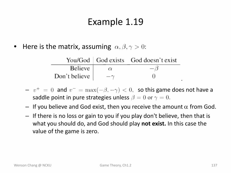
• Here is the matrix, assuming
– and so this game does not have a saddle point in pure strategies unless
– If you believe and God exist, then you receive the amount α from God.– If there is no loss or gain to you if you play don't believe, then that is
what you should do, and God should play not exist. In this case the value of the game is zero.
Wenson Chang @ NCKU Game Theory, Ch1.2 137
.
Example 1.19 (cont’d)
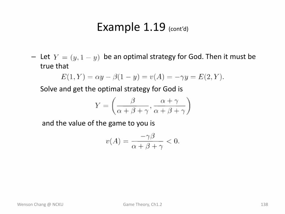
– Let be an optimal strategy for God. Then it must be true that
Solve and get the optimal strategy for God is
and the value of the game to you is
Wenson Chang @ NCKU Game Theory, Ch1.2 138
– Your optimal strategy must satisfy
– If the penalty to you if you don't believe and God exists is loss of eternal life, represented by a very large number. In this case, the percent of time you play believe, should be fairly close to 1, so you should play believe with high probability.
– If this is a zero sum game, God would then play doesn't exist with high probability.
• It may not make much sense to think of this as a zero sum game.
• Maybe we should just look at this like a best response for you, rather than as a zero sum game.
Wenson Chang @ NCKU Game Theory, Ch1.2 139
Example 1.19 (cont’d)
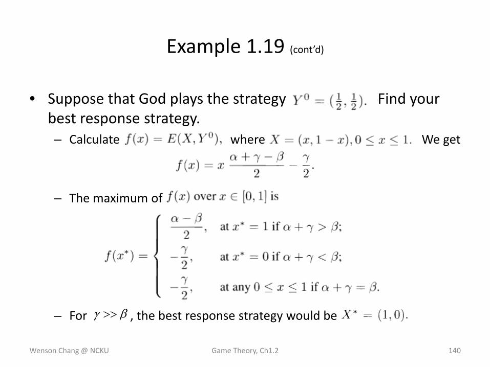
• Suppose that God plays the strategy Find your best response strategy.– Calculate where We get
– The maximum of
– For , the best response strategy would be
Wenson Chang @ NCKU Game Theory, Ch1.2 140
Example 1.19 (cont’d)
βγ >>


![[2007] Advanced Game Theory – Two Person Zero Sum Games](https://static.fdocuments.in/doc/165x107/563db9d9550346aa9aa08151/2007-advanced-game-theory-two-person-zero-sum-games.jpg)