CHAPTER 5k-NEAREST NEIGHBORALGORITHM

SUPERVISED VERSUS UNSUPERVISED METHODS

METHODOLOGY FOR SUPERVISED MODELING

BIAS–VARIANCE TRADE-OFF

CLASSIFICATION TASK

k-NEAREST NEIGHBOR ALGORITHM

DISTANCE FUNCTION

COMBINATION FUNCTION

QUANTIFYING ATTRIBUTE RELEVANCE: STRETCHING THE AXES

DATABASE CONSIDERATIONS

k-NEAREST NEIGHBOR ALGORITHM FOR ESTIMATION AND PREDICTION

CHOOSING k

SUPERVISED VERSUS UNSUPERVISED METHODS

Data mining methods may be categorized as either supervised or unsupervised. Inunsupervised methods, no target variable is identified as such. Instead, the data miningalgorithm searches for patterns and structure among all the variables. The most com-mon unsupervised data mining method is clustering, our topic in Chapters 8 and 9. Forexample, political consultants may analyze congressional districts using clusteringmethods, to uncover the locations of voter clusters that may be responsive to a par-ticular candidate’s message. In this case, all appropriate variables (e.g., income, race,gender) would be input to the clustering algorithm, with no target variable specified,in order to develop accurate voter profiles for fund-raising and advertising purposes.

Another data mining method, which may be supervised or unsupervised, isassociation rule mining. In market basket analysis, for example, one may simply be

Discovering Knowledge in Data: An Introduction to Data Mining, By Daniel T. LaroseISBN 0-471-66657-2 Copyright C© 2005 John Wiley & Sons, Inc.

90

METHODOLOGY FOR SUPERVISED MODELING 91

interested in “which items are purchased together,” in which case no target variablewould be identified. The problem here, of course, is that there are so many itemsfor sale, that searching for all possible associations may present a daunting task, dueto the resulting combinatorial explosion. Nevertheless, certain algorithms, such asthe a priori algorithm, attack this problem cleverly, as we shall see when we coverassociation rule mining in Chapter 10.

Most data mining methods are supervised methods, however, meaning that (1)there is a particular prespecified target variable, and (2) the algorithm is given manyexamples where the value of the target variable is provided, so that the algorithmmay learn which values of the target variable are associated with which values of thepredictor variables. For example, the regression methods of Chapter 4 are supervisedmethods, since the observed values of the response variable y are provided to theleast-squares algorithm, which seeks to minimize the squared distance between thesey values and the y values predicted given the x-vector. All of the classification methodswe examine in Chapters 5 to 7 are supervised methods, including decision trees, neuralnetworks, and k-nearest neighbors.

METHODOLOGY FOR SUPERVISED MODELING

Most supervised data mining methods apply the following methodology for buildingand evaluating a model. First, the algorithm is provided with a training set of data,which includes the preclassified values of the target variable in addition to the predictorvariables. For example, if we are interested in classifying income bracket, based onage, gender, and occupation, our classification algorithm would need a large pool ofrecords, containing complete (as complete as possible) information about every field,including the target field, income bracket. In other words, the records in the trainingset need to be preclassified. A provisional data mining model is then constructed usingthe training samples provided in the training data set.

However, the training set is necessarily incomplete; that is, it does not includethe “new” or future data that the data modelers are really interested in classifying.Therefore, the algorithm needs to guard against “memorizing” the training set andblindly applying all patterns found in the training set to the future data. For example,it may happen that all customers named “David” in a training set may be in the high-income bracket. We would presumably not want our final model, to be applied to newdata, to include the pattern “If the customer’s first name is David, the customer has ahigh income.” Such a pattern is a spurious artifact of the training set and needs to beverified before deployment.

Therefore, the next step in supervised data mining methodology is to examinehow the provisional data mining model performs on a test set of data. In the testset, a holdout data set, the values of the target variable are hidden temporarily fromthe provisional model, which then performs classification according to the patternsand structure it learned from the training set. The efficacy of the classifications arethen evaluated by comparing them against the true values of the target variable. Theprovisional data mining model is then adjusted to minimize the error rate on the testset.

92 CHAPTER 5 k-NEAREST NEIGHBOR ALGORITHM

Use training set to generatea provisional data mining

model.

Apply provisional modelto test set.

Adjust provisional modelto minimize error rate

on test set.

Training set(preclassified)

Test set

"Final"data mining

model

Provisionaldata mining

model

Validation set

Adjusteddata mining

model

Apply adjusted modelto validation set.

Adjust the adjusted modelto minimize error rate on

validation set.

Figure 5.1 Methodology for supervised modeling.

The adjusted data mining model is then applied to a validation data set, anotherholdout data set, where the values of the target variable are again hidden temporarilyfrom the model. The adjusted model is itself then adjusted, to minimize the error rateon the validation set. Estimates of model performance for future, unseen data canthen be computed by observing various evaluative measures applied to the validationset. Such model evaluation techniques are covered in Chapter 11. An overview of thismodeling process for supervised data mining is provided in Figure 5.1.

Usually, the accuracy of the provisional model is not as high on the test or vali-dation sets as it is on the training set, often because the provisional model is overfittingon the training set. Overfitting results when the provisional model tries to account forevery possible trend or structure in the training set, even idiosyncratic ones such as the“David” example above. There is an eternal tension in model building between modelcomplexity (resulting in high accuracy on the training set) and generalizability to thetest and validation sets. Increasing the complexity of the model in order to increasethe accuracy on the training set eventually and inevitably leads to a degradation inthe generalizability of the provisional model to the test and validation sets, as shownin Figure 5.2.

Figure 5.2 shows that as the provisional model begins to grow in complexityfrom the null model (with little or no complexity), the error rates on both the trainingset and the validation set fall. As the model complexity increases, the error rate on the

BIAS–VARIANCE TRADE-OFF 93

Err

or R

ate

Complexity of Model

Error Rate onTraining Set

Error Rate onValidation Set

Underfitting

Optimal Level ofModel Complexity

Overfitting

Figure 5.2 The optimal level of model complexity is at the minimum error rate on thevalidation set.

training set continues to fall in a monotone fashion. However, as the model complexityincreases, the validation set error rate soon begins to flatten out and increase becausethe provisional model has memorized the training set rather than leaving room forgeneralizing to unseen data. The point where the minimal error rate on the validationset is encountered is the optimal level of model complexity, as indicated in Figure 5.2.Complexity greater than this is considered to be overfitting; complexity less than thisis considered to be underfitting.

BIAS–VARIANCE TRADE-OFF

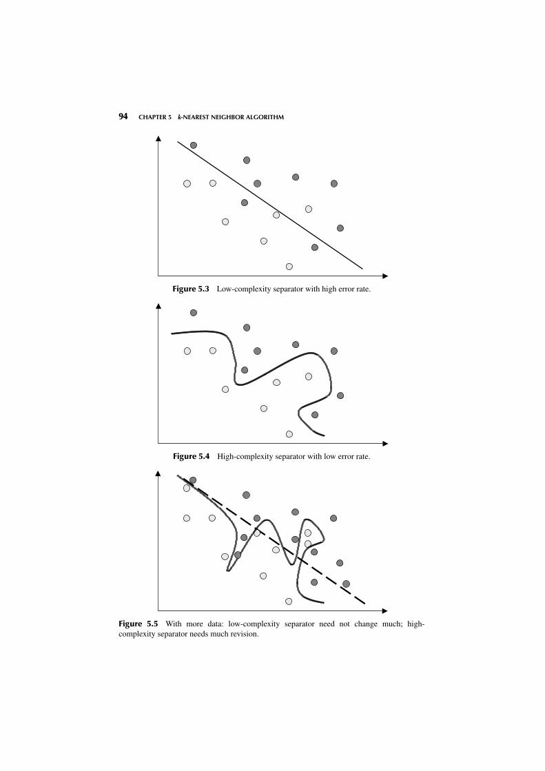
Suppose that we have the scatter plot in Figure 5.3 and are interested in constructingthe optimal curve (or straight line) that will separate the dark gray points from thelight gray points. The straight line in has the benefit of low complexity but suffersfrom some classification errors (points ending up on the wrong side of the line).

In Figure 5.4 we have reduced the classification error to zero but at the cost ofa much more complex separation function (the curvy line). One might be tempted toadopt the greater complexity in order to reduce the error rate. However, one shouldbe careful not to depend on the idiosyncrasies of the training set. For example, sup-pose that we now add more data points to the scatter plot, giving us the graph inFigure 5.5.

Note that the low-complexity separator (the straight line) need not change verymuch to accommodate the new data points. This means that this low-complexityseparator has low variance. However, the high-complexity separator, the curvy line,must alter considerably if it is to maintain its pristine error rate. This high degree ofchange indicates that the high-complexity separator has a high variance.

94 CHAPTER 5 k-NEAREST NEIGHBOR ALGORITHM

Figure 5.3 Low-complexity separator with high error rate.

Figure 5.4 High-complexity separator with low error rate.

Figure 5.5 With more data: low-complexity separator need not change much; high-complexity separator needs much revision.

CLASSIFICATION TASK 95

Even though the high-complexity model has a low bias (in terms of the errorrate on the training set), it has a high variance; And even though the low-complexitymodel has a high bias, it has a low variance. This is what is known as the bias–variance trade-off. The bias–variance trade-off is another way of describing the over-fitting/underfitting dilemma shown in Figure 5.2. As model complexity increases, thebias on the training set decreases but the variance increases. The goal is to construct amodel in which neither the bias nor the variance is too high, but usually, minimizingone tends to increase the other.

For example, the most common method of evaluating how accurate model esti-mation is proceeding is to use the mean-squared error (MSE). Between two competingmodels, one may select the better model as that model with the lower MSE. Why isMSE such a good evaluative measure? Because it combines both bias and variance.The mean-squared error is a function of the estimation error (SSE) and the modelcomplexity (e.g., degrees of freedom). It can be shown (e.g., Hand et al. [1]) that themean-squared error can be partitioned using the following equation, which clearlyindicates the complementary relationship between bias and variance:

MSE = variance + bias2

CLASSIFICATION TASK

Perhaps the most common data mining task is that of classification. Examples ofclassification tasks may be found in nearly every field of endeavor:

� Banking: determining whether a mortgage application is a good or bad creditrisk, or whether a particular credit card transaction is fraudulent

� Education: placing a new student into a particular track with regard to specialneeds

� Medicine: diagnosing whether a particular disease is present� Law: determining whether a will was written by the actual person deceased or

fraudulently by someone else� Homeland security: identifying whether or not certain financial or personal

behavior indicates a possible terrorist threat

In classification, there is a target categorical variable, (e.g., income bracket),which is partitioned into predetermined classes or categories, such as high income,middle income, and low income. The data mining model examines a large set ofrecords, each record containing information on the target variable as well as a setof input or predictor variables. For example, consider the excerpt from a data setshown in Table 5.1. Suppose that the researcher would like to be able to classifythe income bracket of persons not currently in the database, based on the othercharacteristics associated with that person, such as age, gender, and occupation.This task is a classification task, very nicely suited to data mining methods andtechniques.

96 CHAPTER 5 k-NEAREST NEIGHBOR ALGORITHM

TABLE 5.1 Excerpt from Data Set for Classifying Income

Subject Age Gender Occupation Income Bracket

001 47 F Software engineer High

002 28 M Marketing consultant Middle

003 35 M Unemployed Low...

The algorithm would proceed roughly as follows. First, examine the data setcontaining both the predictor variables and the (already classified) target variable,income bracket. In this way, the algorithm (software) “learns about” which com-binations of variables are associated with which income brackets. For example,older females may be associated with the high-income bracket. This data set iscalled the training set. Then the algorithm would look at new records for whichno information about income bracket is available. Based on the classifications inthe training set, the algorithm would assign classifications to the new records. Forexample, a 63-year-old female professor might be classified in the high-incomebracket.

k-NEAREST NEIGHBOR ALGORITHM

The first algorithm we shall investigate is the k-nearest neighbor algorithm, whichis most often used for classification, although it can also be used for estimation andprediction. k-Nearest neighbor is an example of instance-based learning, in whichthe training data set is stored, so that a classification for a new unclassified recordmay be found simply by comparing it to the most similar records in the training set.Let’s consider an example.

Recall the example from Chapter 1 where we were interested in classifying thetype of drug a patient should be prescribed, based on certain patient characteristics,such as the age of the patient and the patient’s sodium/potassium ratio. For a sampleof 200 patients, Figure 5.6 presents a scatter plot of the patients’ sodium/potassium(Na/K) ratio against the patients’ age. The particular drug prescribed is symbolizedby the shade of the points. Light gray points indicate drug Y; medium gray pointsindicate drug A or X; dark gray points indicate drug B or C.

Now suppose that we have a new patient record, without a drug classification,and would like to classify which drug should be prescribed for the patient based onwhich drug was prescribed for other patients with similar attributes. Identified as “newpatient 1,” this patient is 40 years old and has a Na/K ratio of 29, placing her at thecenter of the circle indicated for new patient 1 in Figure 5.6. Which drug classificationshould be made for new patient 1? Since her patient profile places her deep into asection of the scatter plot where all patients are prescribed drug Y, we would thereby

k-NEAREST NEIGHBOR ALGORITHM 97

Age

Na/

K R

atio

10

10

20

30

40

20 30 40 50 60 70

New Patient 1 New Patient 2 New Patient 3

Figure 5.6 Scatter plot of sodium/potassium ratio against age, with drug overlay.

classify new patient 1 as drug Y. All of the points nearest to this point, that is, allof the patients with a similar profile (with respect to age and Na/K ratio) have beenprescribed the same drug, making this an easy classification.

Next, we move to new patient 2, who is 17 years old with a Na/K ratio of12.5. Figure 5.7 provides a close-up view of the training data points in the localneighborhood of and centered at new patient 2. Suppose we let k = 1 for our k-nearestneighbor algorithm, so that new patient 2 would be classified according to whicheversingle (one) observation it was closest to. In this case, new patient 2 would be classified

A

New

C

B

Figure 5.7 Close-up of three nearest neighbors to new patient 2.

98 CHAPTER 5 k-NEAREST NEIGHBOR ALGORITHM

Figure 5.8 Close-up of three nearest neighbors to new patient 2.

for drugs B and C (dark gray), since that is the classification of the point closest tothe point on the scatter plot for new patient 2.

However, suppose that we now let k = 2 for our k-nearest neighbor algorithm,so that new patient 2 would be classified according to the classification of the k = 2points closest to it. One of these points is dark gray, and one is medium gray, so thatour classifier would be faced with a decision between classifying new patient 2 fordrugs B and C (dark gray) or drugs A and X (medium gray). How would the classifierdecide between these two classifications? Voting would not help, since there is onevote for each of two classifications.

Voting would help, however, if we let k = 3 for the algorithm, so that new patient2 would be classified based on the three points closest to it. Since two of the three clos-est points are medium gray, a classification based on voting would therefore choosedrugs A and X (medium gray) as the classification for new patient 2. Note that theclassification assigned for new patient 2 differed based on which value we chose for k.

Finally, consider new patient 3, who is 47 years old and has a Na/K ratio of13.5. Figure 5.8 presents a close-up of the three nearest neighbors to new patient 3.For k = 1, the k-nearest neighbor algorithm would choose the dark gray (drugs B andC) classification for new patient 3, based on a distance measure. For k = 2, however,voting would not help. But voting would not help for k = 3 in this case either, sincethe three nearest neighbors to new patient 3 are of three different classifications.

This example has shown us some of the issues involved in building a classifierusing the k-nearest neighbor algorithm. These issues include:

� How many neighbors should we consider? That is, what is k?� How do we measure distance?� How do we combine the information from more than one observation?

Later we consider other questions, such as:

� Should all points be weighted equally, or should some points have more influ-ence than others?

DISTANCE FUNCTION 99

DISTANCE FUNCTION

We have seen above how, for a new record, the k-nearest neighbor algorithm assignsthe classification of the most similar record or records. But just how do we definesimilar? For example, suppose that we have a new patient who is a 50-year-old male.Which patient is more similar, a 20-year-old male or a 50-year-old female?

Data analysts define distance metrics to measure similarity. A distance metricor distance function is a real-valued function d, such that for any coordinates x , y,and z:

1. d(x,y) ≥ 0, and d(x,y) = 0 if and only if x = y

2. d(x,y) = d(y,x)

3. d(x,z) ≤ d(x,y) + d(y,z)

Property 1 assures us that distance is always nonnegative, and the only way fordistance to be zero is for the coordinates (e.g., in the scatter plot) to be the same.Property 2 indicates commutativity, so that, for example, the distance from New Yorkto Los Angeles is the same as the distance from Los Angeles to New York. Finally,property 3 is the triangle inequality, which states that introducing a third point cannever shorten the distance between two other points.

The most common distance function is Euclidean distance, which representsthe usual manner in which humans think of distance in the real world:

dEuclidean(x,y) =√∑

i

(xi − yi )2

where x = x1, x2, . . . , xm , and y = y1, y2, . . . , ym represent the m attribute values oftwo records. For example, suppose that patient A is x1 = 20 years old and has a Na/Kratio of x2 = 12, while patient B is y1 = 30 years old and has a Na/K ratio of y2 = 8.Then the Euclidean distance between these points, as shown in Figure 5.9, is

dEuclidean(x,y) =√∑

i

(xi − yi )2 =√

(20 − 30)2 + (12 − 8)2

=√

100 + 16 = 10.77

Na/

K R

atio (20, 12)

(30, 8)

Age

Figure 5.9 Euclidean distance.

100 CHAPTER 5 k-NEAREST NEIGHBOR ALGORITHM

When measuring distance, however, certain attributes that have large values,such as income, can overwhelm the influence of other attributes which are measuredon a smaller scale, such as years of service. To avoid this, the data analyst shouldmake sure to normalize the attribute values.

For continuous variables, the min–max normalization or Z-score standardiza-tion, discussed in Chapter 2, may be used:

Min–max normalization:

X∗ =X − min(X )

range(X)=

X − min(X )

max(X) − min(X)

Z-score standardization:

X∗ =X − mean(X )

SD(X )

For categorical variables, the Euclidean distance metric is not appropriate. Instead,we may define a function, “different from,” used to compare the i th attribute valuesof a pair of records, as follows:

different(xi ,yi ) ={

0 if xi = yi

1 otherwise

where xi and yi are categorical values. We may then substitute different (x ,i yi ) for the

ith term in the Euclidean distance metric above.For example, let’s find an answer to our earlier question: Which patient is more

similar to a 50-year-old male: a 20-year-old male or a 50-year-old female? Supposethat for the age variable, the range is 50, the minimum is 10, the mean is 45, and thestandard deviation is 15. Let patient A be our 50-year-old male, patient B the 20-year-old male, and patient C the 50-year-old female. The original variable values, alongwith the min–max normalization (ageMMN ) and Z -score standardization (ageZscore),are listed in Table 5.2.

We have one continuous variable (age, x1) and one categorical variable (gender,x2). When comparing patients A and B, we have different (x2,y2) = 0, withdifferent (x2,y2) = 1 for the other combinations of patients. First, let’s see what hap-pens when we forget to normalize the age variable. Then the distance between patientsA and B is d(A,B) =

√(50 − 20)2 + 02 = 30, and the distance between patients A

and C is d(A,C) =√

(20 − 20)2 + 12 = 1. We would thus conclude that the 20-year-old male is 30 times more “distant” from the 50-year-old male than the 50-year-old

TABLE 5.2 Variable Values for Age and Gender

Patient Age AgeMMN AgeZscore Gender

A 5050 − 10

50= 0.8

50 − 45

15= 0.33 Male

B 2020 − 10

50= 0.2

20 − 45

15= −1.67 Male

C 5050 − 10

50= 0.8

50 − 45

15= 0.33 Female

COMBINATION FUNCTION 101

female is. In other words, the 50-year-old female is 30 times more “similar” to the50-year-old male than the 20-year-old male is. Does this seem justified to you? Well,in certain circumstances, it may be justified, as in certain age-related illnesses. But,in general, one may judge that the two men are just as similar as are the two 50-year-olds. The problem is that the age variable is measured on a larger scale than theDifferent(x2,y2) variable. Therefore, we proceed to account for this discrepancy bynormalizing and standardizing the age values, as shown in Table 5.2.

Next, we use the min–max normalization values to find which patient ismore similar to patient A. We have dMMN(A,B) =

√(0.8 − 0.2)2 + 02 = 0.6 and

dMMN(A,C) =√

(0.8 − 0.8)2 + 12 = 1.0, which means that patient B is now consid-ered to be more similar to patient A.

Finally, we use the Z -score standardization values to determine which patient ismore similar to patient A. We have dZscore(A,B) =

√[0.33 − (−1.67)]2 + 02 = 2.0

and dZscore(A,C) =√

(0.33 − 0.33)2 + 12 = 1.0, which means that patient C is againcloser. Using the Z -score standardization rather than the min–max standardizationhas reversed our conclusion about which patient is considered to be more similar topatient A. This underscores the importance of understanding which type of normal-ization one is using. The min–max normalization will almost always lie between zeroand 1 just like the “identical” function. The Z -score standardization, however, usuallytakes values −3 < z < 3, representing a wider scale than that of the min–max nor-malization. Therefore, perhaps, when mixing categorical and continuous variables,the min–max normalization may be preferred.

COMBINATION FUNCTION

Now that we have a method of determining which records are most similar to the new,unclassified record, we need to establish how these similar records will combine toprovide a classification decision for the new record. That is, we need a combinationfunction. The most basic combination function is simple unweighted voting.

Simple Unweighted Voting1. Before running the algorithm, decide on the value of k, that is, how many records

will have a voice in classifying the new record.

2. Then, compare the new record to the k nearest neighbors, that is, to the k recordsthat are of minimum distance from the new record in terms of the Euclideandistance or whichever metric the user prefers.

3. Once the k records have been chosen, then for simple unweighted voting, theirdistance from the new record no longer matters. It is simple one record, onevote.

We observed simple unweighted voting in the examples for Figures 5.4 and 5.5.In Figure 5.4, for k = 3, a classification based on simple voting would choose drugsA and X (medium gray) as the classification for new patient 2, since two of the threeclosest points are medium gray. The classification would then be made for drugs Aand X, with confidence 66.67%, where the confidence level represents the count ofrecords, with the winning classification divided by k.

102 CHAPTER 5 k-NEAREST NEIGHBOR ALGORITHM

On the other hand, in Figure 5.5, for k = 3, simple voting would fail to choosea clear winner since each of the three categories receives one vote. There would be atie among the three classifications represented by the records in Figure 5.5, and a tiemay not be a preferred result.

Weighted Voting

One may feel that neighbors that are closer or more similar to the new record shouldbe weighted more heavily than more distant neighbors. For example, in Figure 5.5,does it seem fair that the light gray record farther away gets the same vote as thedark gray vote that is closer to the new record? Perhaps not. Instead, the analyst maychoose to apply weighted voting, where closer neighbors have a larger voice in theclassification decision than do more distant neighbors. Weighted voting also makesit much less likely for ties to arise.

In weighted voting, the influence of a particular record is inversely proportionalto the distance of the record from the new record to be classified. Let’s look at anexample. Consider Figure 5.6, where we are interested in finding the drug classifica-tion for a new record, using the k = 3 nearest neighbors. Earlier, when using simpleunweighted voting, we saw that there were two votes for the medium gray classifica-tion, and one vote for the dark gray. However, the dark gray record is closer than theother two records. Will this greater proximity be enough for the influence of the darkgray record to overcome that of the more numerous medium gray records?

Assume that the records in question have the values for age and Na/K ratiogiven in Table 5.3, which also shows the min–max normalizations for these values.Then the distances of records A, B, and C from the new record are as follows:

d(new,A) =√

(0.05 − 0.0467)2 + (0.25 − 0.2471)2 = 0.004393

d(new,B) =√

(0.05 − 0.0533)2 + (0.25 − 0.1912)2 = 0.58893

d(new,C) =√

(0.05 − 0.0917)2 + (0.25 − 0.2794)2 = 0.051022

The votes of these records are then weighted according to the inverse square of theirdistances.

One record (A) votes to classify the new record as dark gray (drugs B and C),so the weighted vote for this classification is

TABLE 5.3 Age and Na/K Ratios for Records from Figure 5.4

Record Age Na/K AgeMMN Na/KMMN

New 17 12.5 0.05 0.25

A (dark gray) 16.8 12.4 0.0467 0.2471

B (medium gray) 17.2 10.5 0.0533 0.1912

C (medium gray) 19.5 13.5 0.0917 0.2794

QUANTIFYING ATTRIBUTE RELEVANCE: STRETCHING THE AXES 103

votes (dark gray) =1

d(new,A)2 =1

0.0043932 51,818

Two records (B and C) vote to classify the new record as medium gray (drugs A andX), so the weighted vote for this classification is

votes (medium gray) =1

d(new,B)2 +1

d(new,C)2 =1

0.0588932+

1

0.0510222

672

Therefore, by the convincing total of 51,818 to 672, the weighted voting procedurewould choose dark gray (drugs B and C) as the classification for a new 17-year-oldpatient with a sodium/potassium ratio of 12.5. Note that this conclusion reverses theearlier classification for the unweighted k = 3 case, which chose the medium grayclassification.

When the distance is zero, the inverse would be undefined. In this case thealgorithm should choose the majority classification of all records whose distance iszero from the new record.

Consider for a moment that once we begin weighting the records, there is notheoretical reason why we couldn’t increase k arbitrarily so that all existing records areincluded in the weighting. However, this runs up against the practical considerationof very slow computation times for calculating the weights of all of the records everytime a new record needs to be classified.

QUANTIFYING ATTRIBUTE RELEVANCE:STRETCHING THE AXES

Consider that not all attributes may be relevant to the classification. In decision trees(Chapter 6), for example, only those attributes that are helpful to the classification areconsidered. In the k-nearest neighbor algorithm, the distances are by default calculatedon all the attributes. It is possible, therefore, for relevant records that are proximateto the new record in all the important variables, but are distant from the new recordin unimportant ways, to have a moderately large distance from the new record, andtherefore not be considered for the classification decision. Analysts may thereforeconsider restricting the algorithm to fields known to be important for classifying newrecords, or at least to blind the algorithm to known irrelevant fields.

Alternatively, rather than restricting fields a priori, the data analyst may prefer toindicate which fields are of more or less importance for classifying the target variable.This can be accomplished using a cross-validation approach or one based on domainexpert knowledge. First, note that the problem of determining which fields are moreor less important is equivalent to finding a coefficient z j by which to multiply thejth axis, with larger values of z j associated with more important variable axes. Thisprocess is therefore termed stretching the axes.

The cross-validation approach then selects a random subset of the data to beused as a training set and finds the set of values z1, z2, . . . zm that minimize theclassification error on the test data set. Repeating the process will lead to a more

104 CHAPTER 5 k-NEAREST NEIGHBOR ALGORITHM

accurate set of values z1, z2, . . . zm . Otherwise, domain experts may be called uponto recommend a set of values for z1, z2, . . . zm . In this way, the k-nearest neighboralgorithm may be made more precise.

For example, suppose that either through cross-validation or expert knowl-edge, the Na/K ratio was determined to be three times as important as age fordrug classification. Then we would have zNa/K = 3 and zage = 1. For the exampleabove, the new distances of records A, B, and C from the new record would be asfollows:

d(new,A) =√

(0.05 − 0.0467)2 + [3(0.25 − 0.2471)]2 = 0.009305

d(new,B) =√

(0.05 − 0.0533)2 + [3(0.25 − 0.1912)]2 = 0.17643

d(new,C) =√

(0.05 − 0.0917)2 + [3(0.25 − 0.2794)]2 = 0.09756

In this case, the classification would not change with the stretched axis for Na/K,remaining dark gray. In real-world problems, however, axis stretching can lead to moreaccurate classifications, since it represents a method for quantifying the relevance ofeach variable in the classification decision.

DATABASE CONSIDERATIONS

For instance-based learning methods such as the k-nearest neighbor algorithm, it isvitally important to have access to a rich database full of as many different combina-tions of attribute values as possible. It is especially important that rare classificationsbe represented sufficiently, so that the algorithm does not only predict common clas-sifications. Therefore, the data set would need to be balanced, with a sufficiently largepercentage of the less common classifications. One method to perform balancing isto reduce the proportion of records with more common classifications.

Maintaining this rich database for easy access may become problematic ifthere are restrictions on main memory space. Main memory may fill up, and accessto auxiliary storage is slow. Therefore, if the database is to be used for k-nearestneighbor methods only, it may be helpful to retain only those data points that arenear a classification “boundary.” For example, in Figure 5.6, all records with Na/Kratio value greater than, say, 19 could be omitted from the database without loss ofclassification accuracy, since all records in this region are classified as light gray. Newrecords with Na/K ratio > 19 would therefore be classified similarly.

k-NEAREST NEIGHBOR ALGORITHM FORESTIMATION AND PREDICTION

So far we have considered how to use the k-nearest neighbor algorithm for classifica-tion. However, it may be used for estimation and prediction as well as for continuous-valued target variables. One method for accomplishing this is called locally weighted

CHOOSING k 105

TABLE 5.4 k = 3 Nearest Neighbors of the New Record

Record Age Na/K BP AgeMMN Na/KMMN Distance

New 17 12.5 ? 0.05 0.25 —

A 16.8 12.4 120 0.0467 0.2471 0.009305

B 17.2 10.5 122 0.0533 0.1912 0.16783

C 19.5 13.5 130 0.0917 0.2794 0.26737

averaging. Assume that we have the same data set as the example above, but this timerather than attempting to classify the drug prescription, we are trying to estimate thesystolic blood pressure reading (BP, the target variable) of the patient, based on thatpatient’s age and Na/K ratio (the predictor variables). Assume that BP has a range of80 with a minimum of 90 in the patient records.

In this example we are interested in estimating the systolic blood pressurereading for a 17-year-old patient with a Na/K ratio of 12.5, the same new patientrecord for which we earlier performed drug classification. If we let k = 3, we havethe same three nearest neighbors as earlier, shown here in Table 5.4. Assume that weare using the zNa/K = three-axis-stretching to reflect the greater importance of theNa/K ratio.

Locally weighted averaging would then estimate BP as the weighted averageof BP for the k = 3 nearest neighbors, using the same inverse square of the distancesfor the weights that we used earlier. That is, the estimated target value y is calculatedas

ynew =

∑i

wi yi

∑i

wi

where wi = 1/d(new, xi )2 for existing records x1, x2, . . . , xk . Thus, in this example,the estimated systolic blood pressure reading for the new record would be

ynew =

∑i

wi yi

∑i

wi=

1200.0093052 + 122

0.176432 + 1300.097562

10.0093052 + 1

0.176432 + 10.097562

= 120.0954.

As expected, the estimated BP value is quite close to the BP value in the present dataset that is much closer (in the stretched attribute space) to the new record. In otherwords, since record A is closer to the new record, its BP value of 120 contributesgreatly to the estimation of the BP reading for the new record.

CHOOSING k

How should one go about choosing the value of k? In fact, there may not be anobvious best solution. Consider choosing a small value for k. Then it is possiblethat the classification or estimation may be unduly affected by outliers or unusual

106 CHAPTER 5 k-NEAREST NEIGHBOR ALGORITHM

observations (“noise”). With small k (e.g., k = 1), the algorithm will simply returnthe target value of the nearest observation, a process that may lead the algorithm towardoverfitting, tending to memorize the training data set at the expense of generalizability.

On the other hand, choosing a value of k that is not too small will tend to smoothout any idiosyncratic behavior learned from the training set. However, if we take thistoo far and choose a value of k that is too large, locally interesting behavior will beoverlooked. The data analyst needs to balance these considerations when choosingthe value of k.

It is possible to allow the data itself to help resolve this problem, by followinga cross-validation procedure similar to the earlier method for finding the optimalvalues z1, z2, . . . zm for axis stretching. Here we would try various values of k withdifferent randomly selected training sets and choose the value of k that minimizes theclassification or estimation error.

REFERENCE1. David Hand, Heikki Mannila, and Padhraic Smyth, 2001, Principles of Data Mining, MIT

Press, Cambridge, MA, 2001.

EXERCISES1. Explain the difference between supervised and unsupervised methods. Which data mining

tasks are associated with unsupervised methods? Supervised? Both?

2. Describe the differences between the training set, test set, and validation set.

3. Should we strive for the highest possible accuracy with the training set? Why or why not?How about the validation set?

4. How is the bias–variance trade-off related to the issue of overfitting and underfitting? Ishigh bias associated with overfitting and underfitting, and why? High variance?

5. What is meant by the term instance-based learning?

6. Make up a set of three records, each with two numeric predictor variables and one cate-gorical target variable, so that the classification would not change regardless of the valueof k.

7. Refer to Exercise 6. Alter your data set so that the classification changes for differentvalues of k.

8. Refer to Exercise 7. Find the Euclidean distance between each pair of points. Using thesepoints, verify that Euclidean distance is a true distance metric.

9. Compare the advantages and drawbacks of unweighted versus weighted voting.

10. Why does the database need to be balanced?

11. The example in the text regarding using the k-nearest neighbor algorithm for estimation hasthe closest record, overwhelming the other records in influencing the estimation. Suggesttwo creative ways that we could dilute this strong influence of the closest record.

12. Discuss the advantages and drawbacks of using a small value versus a large value for k.