Risk Management in the Iullemeden Aquifer System - Abdel Kader Dodo - Iullemeden Aquifer
Techniques of Water-Resources Investigations of the United States Geological Survey
Chapter Cl
FINITE-DIFFERENCE MODEL FOR 0 AQUIFER SIMULATION IN
TWO DIMENSIONS WITH RESULTS OF
NUMERICAL EXPERIMENTS
By P. C. Trescott, G. F. Pinder, and S. P. Larson
Book 7
AUTOMATED DATA PROCESSING AND COMPUTATIONS
UNITED STATES DEPARTMENT OF TWE INTERIOR
CECIL D. ANDRUS, Secretary
GEOLOGICAL SUR\IEY
H. VVilliam Menard, Director
First printing 1976
Second printing 1980
Requests, at cost, for the Card Deck listed in Attachment VII should be directed to: Ralph N. Either, Chief, Office of Teleprocessing, M.S. 805, National Center,
U.S. Geological Survey, Reston, Virginia 22092.
UNITED STATES GOVERNMENT PRINTING OFFICE, WASHINGTON : 1976
For sale by the Branch of Distribution, U.S. Geological Survey, 1200 South Eads Street, Arlington, VA 22202
PREFACE
The series of manuals on techniques describes procedures for plan- ning and executing specialized work in water-resources investigations. The material is grouped under major headings called books and further sub- divided into sections and chapters; section C of Book ‘7 is on computer programs.
“Finite-difference model for aquifer simulation in two dimensions with results of numerical experiments” supersedes the report published in 1970 entitled, “A digital model for aquifer evaluation” by G. F. Pinder as Chapter Cl of Book 7. The new Chapter Cl represents a significant im- provement in the computational capability to solve the flow equations and has greater flexibility in the hydrologic situations that can be simulated.
III
l
CONTENTS
Abstract _________________________________ Introduction ______________________________ Theoretical development ____________-______
Ground-water flow equation ____________ Finite-difference approximations __---__- Source term __________________________
Leakage __________________________ Evapotranspiration ____ ____________
Computation of head at the radius of a pumping well ______________________
Combined artesian-water-table simulation- Transmissivity ------------------- Storage __________________________ Leakage _________________________
Test problems _____________-______________ Numerical solution ________________________
Line successive overrelaxation __________ Two-dimensional correction to LSOR LSOR acceleration parameter ______
Alternating-direction implicit pro- cedure _____________________________
Strongly implicit procedure ____________ Comparison of numerical results ____________ Considerations in designing an aquifer
model __________________________________ Boundary conditions __________________ Initial conditions _____________________ Designing the finite-difference grid _____
Selected references ________________________ Attachment I, notation ____________________ Attachment II, computer program __________
Main program ________________________
Page 1
1 2 2 2 4 4 7
8 10 11 11 11 12 14 15 17 18
19 21 27
29 29 30 30 32 37 38 38
Attachment II, computer program-Continued Subroutine DATA1 ___-_-_-~-~---~~~--~
Time parameters _----------------- Initialization _____________________
Subroutine STEP ____________-________ Maximum head change for each
iteration _______________________ Subroutine SOLVE ___________________
SIP iteration parameters _-_-__---- Exceeding permitted iterations _____
Subroutine COEF ____________________ Transient leakage coefficients ---_-- Transmissivity as a function of
head __________________________ TR and TC coefficients __-_--__--_-
Subroutine CHECK1 __________________ Subroutine PRNTAI __________________ BLOCK DATA routine ____--------~--- Technical Information ___-__----_~---~
Storage requirements ____________-- Computation time ______--__-----_- Use of disk facilities for storage of
array data and interim results __ Graphical display package _------------ Modification of program logic _-----__-- Fortran IV __________________________ Limitations of program ___--__--__-_--
Attachment III, data deck instructions------ Attachment IV, sample aquifer simulation
and job control language ---_------------ Attachment V, generalized flow chart for
aquifer simulation model _____________-__ Attachment VI, definition of program variables Attachment VII, program listing __-__-__-__
FIGURES
1. Index scheme for Anitedifference grid and coefficients of finite-difference equation written for node (i,i) ________________________________________-----------------------------------
2. In the first pumping period, (a) illustrates the head distribution in the confining bed at one time when transient leakage effects are significant; (b) illustrates a time after transient effects have dissipated; in the second pumping period, (c) is analogous to (a) and (d) is analogous to (b) __________________-_____________________------------------------------------------
3. The total drawdown at the elapsed time, t, in the pumping period (a) is applied at t/3 in equa- tions 9 and 10 to approximate qoc,,,r, the transient part of q’,,,,r (b) _- ___________________ -_
Page
38 38 40 40
40 40 41 41 41 41
41 41 42 42 43 43 43 43
44 46 46 46 48 49
66
68 74 78
Page
2
6
6
V
VI I CONTENTS
4.
6.
6.
7. 8.
9. 10. 11.
12. 13. 14.
16.
16.
17. 18. 19.
20. 21. 22. 23. 24. 25. 26. 27. 28.
29. 30.
31.
32. 33.
Comparison of analytic solution and numerical results using factors of 2 and 3 in the transient leakage approximation ________________________________________------------------------
Percent difference between the volume of leakage computed with the model approximation and Hantush’s analytical results _________________------.-------------------------------------
Evapotranspiration decreases linearly from &., where the water table is at land surface to zero where the water table is less than or equal to Gc,&X~ --_---____________________________
Flow from cell (i’l,i) to cell (ii) (a) and equivalent rad*ial flow to well (i,i) with radius rs (b) __ Storage adjustmen i- is applied to distance A in conversion from artesian to water-table conditions
(a) and to distance B in conversbon from water-table to artesian conditions (b) _____-__-__ Two of the possible situations in which leakage is restricted in artesian-water-table simulations _- Characteristics of test problem 1 _________ - _____________ -----_--__--__-- ______________ --___- Transmissivity and observed water-ta.ble configuration for teet problem 2 (fieldwork and model
design by Konikow, 1976) ________________________________________---------------------- Characteristics of test problem 3 ____________________ - __.________ --_--_-- ____________________ Hypothetical problem with 9 interior nodes -- ____ - ____ -_-----_--___- ____________________---- Number of iterations required for solution by LSOR and LSOR + 2DC using different accelera-
tion parameters __________-_-----_-----~~~~~-~----~.~~~~--~~-----~--~~~~~~~~~~~~~~~~~~~~ Reduction in the maximum residual for problems 1 to 3 for selected ~,a,, used to compute the
AD1 parameters ______-_--__---_-_----~~~~~-~-~~~~~~~~~-~~--~~~~--~~~~~~~~~~~~~~~~~~~~ Number of iterations required for solution of the test problems with AD1 using different num-
bers of parameters --_-____________--______________________--------------------------- Coefficients of unknowns in equation 27 ________________________________________-------------- Reverse numbering1 scheme for 3 x 3 problem---- ______________ -___--__-- ____________________ Iterations required ‘for solution of the test problem by SIF’ using different numbers and sequences
of parameters ____---_--_____-________________________-------------------------------- Computational work required by different iterative techniques for problem 1 ___- _______________ Computational work requi’red by different iterative techniques for problem 2 ______ - ____________ Computational work required by different iterative techniques for problem 3 ______--____-__--__ Computational work required by different iterative technisques for problem 4 __________________ Number of iterations required for solution of problem 4 by SIP using different values of p’ --_-_ Variable, block-centered grid with mi zed boundary conditions ___- -_ --_ -_ - -_ __ _ __ _____________ Orientation of manon computer page __- _________ ---_- __________ --___-__--_---------________ Additional FORTRAN code required to produce output for graphical displav __-__-_-________ Water level versus time at various n,odes of the sample aquifer problem produced by the graphi-
cal display padkage _______-____---_-__-____________________--------------------------- Contour map of water level for sample aquifer problem produced by graphical display package _ Cross section illustrates several options included in the sample ,problem and identifies the meaning
of several program parameters ___________________-____________________----------------- JCL and data deck ‘to copy some of the data sets on disk, compute for 5 iterations, and store the re
sults on disk -_-__-__________________________________---------------------------------- JCL and data deck tto continue the previous run (fig. 31) te a solution -- ____ - _____ - _____________ JCL and data deck’ to simulate the sample problem without using disk files _______ - ___________
TABLES
1. Comparison of drawdowns computed with equation 16 and the analytic values _________________ 2. Number of arrays required for the options ____________________ --___-__--___- _____ -__--- _____
Page 0
7
8
9 9
11 12 13
14 15 16
19
22
23 24 25
26 27 28 28 28 28 31
0
43 47
48 49
65
66 57 68
Page 10 38
3. Arrays passed to the subroutines and their relative location in the vector Y ------------------- 39
FINITE-DIFFERENCE MODEL FOR AQUIFER SIMULATION IN TWO DIMENSIONS WITH RESULTS OF
NUMERICAL EXPERIMENTS
By P. C. Trescott, G. F. Pinder, and S. P. Larson
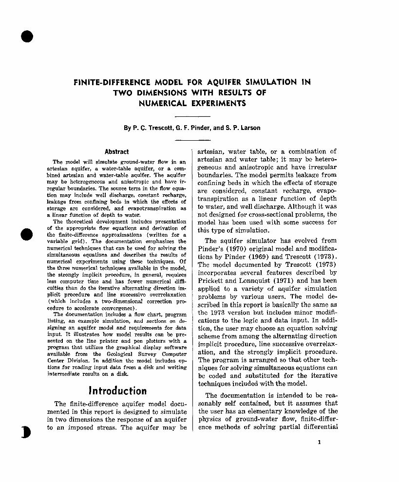
Abstract The model will simulate ground-water flow in an
artesian aquifer, a water-table aquifer, or a com- bined artesian and water-table aquifer. The aquifer may be heterogen,eous and anisotropic and have ir- regular boundaries. The source term in the flow equa- tion may include well discharge, constant recharge, leakage from confining beds in which the effects of storage are considered, and wapotranspiration as a linear function of depth to watex.
The theoretical development includes presentation
0
of the appropriate flow equations and derivation of the finite-difference approximations (written for a variable grid). The documentation emphasizes the numerical techniques that can be used for solving the simultaneous equations and describes the results of numerical experiments using these techniques. Of the three numerical techniques available in the model, the strongly implicit procedure, in general, requires less computer time and has fewer numerical diffi- culties than do the iterative alternating direction im- plicit procedure and line successive overrclaxation (which includes a two-dimensional correction pro- cedure to accelerate convergence).
The documentation includes a flow chart, program listing, an example simulation, and sections on de- signing an aquifer model and requirements for data input. It illustrates how model results can be pre- sented on the line printer and pen plotters with a program that utilizes the graphical display software available from the Geological Survey Computer Center Division. In addition the model includes op- tions for reading input data from a disk and writing intermediate results on a disk.
Introduction The finite-difference aquifer model docu-
mented in this report is designed to simulate in two dimensions the response of an aquifer to an imposed stress. The aquifer may be
artesian, water table, or a combination of artesian and water table ; it may be hetero- geneous and anisotropic and have irregular boundaries. The model permits leakage from confining beds in which the effects of storage are considered, constant recharge, evapo- transpiration as a linear function of depth to water, and well discharge. Although it was not designed for cross-sectional problems, the model has been used with some success for this type of simulation.
The aquifer simulator has evolved from Pinder’s (1970) original model and modifica- tions by Pinder (1969) and Trescott (1973). The model documented by Trescott (1973) incorporates several features described by Prickett and Lonnquist (1971) and has been applied to a variety of aquifer simulation problems by various users. The model de- scribed in this report is basically the same as the 1973 version but includes minor modifi- cations to the logic and data input. In addi- tion, the user may choose an equation solving scheme from among the alternating direction implicit procedure, line successive overrelax- ation, and the strongly implicit procedure. The program is arranged so that other tech- niques for solving simultaneous equations can be coded and substituted for the iterative techniques included with the model.
The documentation is intended to be re;G sonably self contained, but it assumes that the user has an elementary knowledge of the physics of ground-water flow, finite-differ- ence methods of solving partial differential
1
2 T+HNIQUES OF WATER-RESOURCES INVESTIGATIONS
equations, matrix lgebra, and the FOR- TRAN IV language. B
Theoretical Development
Ground-watgr flow equation The partial differential equation of ground-
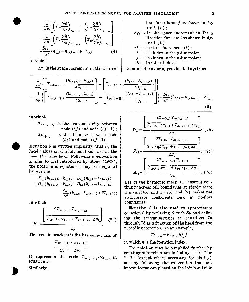
water flow in a confined aquifer in two di- mensions may be written as
in which
W(x, y, t) is the volumetric flux of re-
T,,, T,,, T,,, T&, are the components of
charge or withdrawal per
the transmissivity tensor
unit surface area of the
yt-1) ; h is hydraulic head (L) ;
aquifer (Libl).
S is /the storage coefficient (dimensionless) ;
The reader is referred to Pinder and Brede- hoeft (1968) for development and discussion of equation 1. In the simulation modcel, equa- tion 1 is simplified by assuming that the Cartesian coordinate axes x and y are alined with the principal components of the trans- missivity tensor, T,,iand T,,, giving
In water-table aquifers, transmissivity is a function of head. Assuming that the coordi- nate axes are co-linear with the principal components of the hydraulic conductivity tensor, the flow equation may be expressed as (Bredehoeft and Pinder, 1970)
in which
K,,, ,K,, are the principal components of the hydraulic conductivity tensor (U-l) ;
s, is the specific yield of the aqui- fer (dimensionless) ;
h is the saturated thickness of the aquifer (~5).
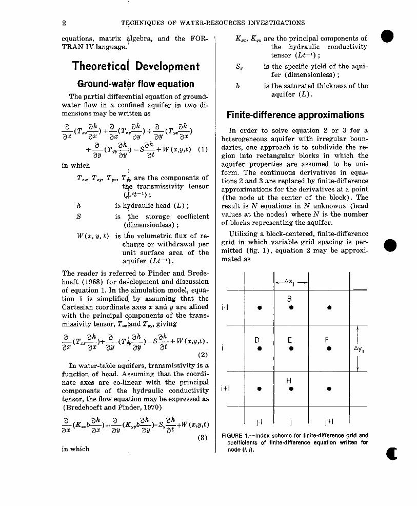
Finite-difference approximations In order to solve equation 2 or 3 for a
Utilizing a block-centered, finite-difference
heterogeneous aquifer with irregular boun-
grid in which variable grid spacing is per-
daries, one approach is to subdivide the re- gion into rectangular blocks in which the
mitted (fig. 1), equation 2 may be approxi-
aquifer properties are assumed to be uni- form. The continuous derivatives in equa- tions 2 and 3 are replaced by finite-difference
mated as
approximations for the derivatives at a point (the node at the center of the block). The result is N equations in N unknowns (head values at the nodes) where N is the number of blocks representing the aquifer.
--
i-l
I
--
i+l
bXJ -I B I
0 a
I D I l
D E F 0 0 0
I I H 0 0 0
j-l I j I jtl
FIGURE l.--Index scheme for finite-difference grid and coefficients of finite-difference equation written for node (i, j).
c
FINITE-DIFFERENCE MODEL FOR AQUIFER SIMULATION 3
+~[(Tu~)i+~,j-~u~)*-,,,3
="s (h,j,k- h,j,k-1) + Wi,j,k (4)
in which
AX] is the space increment in the x direc-
tion for column j as shown in fig- ure 1 (;L);
Ayi is in the space increment in the y direction for row i as shown in fig- ure 1 (G) ;
At is the time increment (t) ; i is the index in the y dimension ; j is the index in the x dimension ; k is the time index.
Equation 4 may be approximated again as
T (kj+l,k-ki.k) I[ _ T (&r- ki-I,k) =o(i,j+%)
AX1+ ?4 IE (i,j-%)
AXi.-% II Tuu (i+%.j) (h+~,j,k--h.j,k) I[ _ T (hij,k--hi-1,j.k)
AYi+. uu +-%A AYi-l/
=g(h,j,k- hi,j,k-1) + wi,j,k
in which
T,, (i,j+j/,) #is the transmissivity between node (i,j) and node (i,j+ 1) ;
Ax i+‘h is the distance between node (i,j) and node (i,j+ 1).
Equation 5 is written implicitly, that is, the head values on the IefLhand side are at the new (k) time level. Following a convention similar to that introduced by Stone (1968), the notation in equation 6 may be simplified by writing
Fi,j(h,j+l,k- h,j,k) -D&j (h,j,k- hi,j--l,k)
+Hi,j(h+l,j,k- k,j,k) -Bi,j (h,j,k-hi-l,j,k)
in which
TV, [t.jl Ayi--1+ Tyy[i-l.jl Ayi 1 (7a) Bi,j=
4% The term in brackets is the harmonic mean of
T ffu Iid Tuu [i-l.il
ay, &hi--~
It represents the ratio TV,+ 5/z,/Ayi-s in equation 5.
l Similarly,
(5)
2Tiom[i.j] Tm [i.j--11
T .m~t,j] AXj-l+ Tmz~i,j-l]AXj 1 Di,i =
AXj ; Ub)
[
2Tm[i,jl Tm [t,j+ll
Tscrnri,jlAX~+1+ Tm [i.j+l]AXj 1 F,j=
AXj ; (7c)
[
2Tuu~i+l.j] Tuu [i.jl
Tuu[i,jl AY4+1 + Tuu[t+l,jlAY,i 1 H4.j =
AY+ . (7d)
Use of the harmonic mean (1) insures con- tinuity across cell boundaries at steady state if a variable grid is used, and (2) makes the appropriate coefficients zero at no-flow boundaries.
Equation 6 is also used to approximate equation 3 by replacing S with Sy and defin- ing the transmissivities in equations 7a through 7d as a function of the head from the preceding iteration. As an example,
Tinci,jJ =K,,~,i,j,bt~~
in which n is the iteration index. The notation may be simplified further by
omitting subscripts not including a “ + 1” or “-1” (except where necessary for clarity) and by following the convention that un- known terms are placed on the left-hand side
4 TlhCHNIQUES OF WATER-RESOURCES INVESTIGATIONS I
of the equations. 4 quation 6 may be rear- ranged and expressed as
Bh-,+Dh,-,+&+Fh,+,+Hhi+l=Q (8) in which I
E=- (B+D+k+H+
Q= -$hx-,+iW.
Souice term The source term I/V(x,y,t) can incl.ude well
discharge, transientlleakage from a confining bed, recharge from ‘precipitation and evapo- transpiration. In the model the source term is computed as I
Wj,j,k = Qw Wkl
Axj Ay.i - qre Ii.j.kl - h,k + qet [i,j,k]
in which 12, Ci,j,LJ is the well discharge (Dt-I) ; ‘&[i,j,k] is the recharge flux per Unit area
(;Lt-1) ; il’i,j,k is the flux per unit area from a
confining layer (Lt-I) ; (I,~ [i,i’,,C1 is the evapotranspiration flux
per unit area (Lt-I).
Leakage
Leakage from a confining layer or stream- bed in which storage is considered may be approxim.ated by
Ki'j h )I) ’ + ---$ b,j,o - k,j,o) (9 1
(K: jt/mi,jS,[ij,) is dimensionless time; see Bredehoeft and Pinder (1970) for a discussion Iof leak- age versus dimen- sionless tim’e ;
t is the elapsed time of I the pumping period
(t) *
in which
ki,i,O
L,j,O
1
1 is the hydraulic head in the aquifer at the start of the pumping
I period (&) ; I is the hydraulic head
Kij >
mi,j
ss[i.jl
I on the other side of the confining bed (L) ;
/ is the hydraulic con- ductivity of the con- fining bed (L/t) ;
is the thickness of the confining bed (L) ;
, is the specific storage in the confining lay- er (L-l) ;
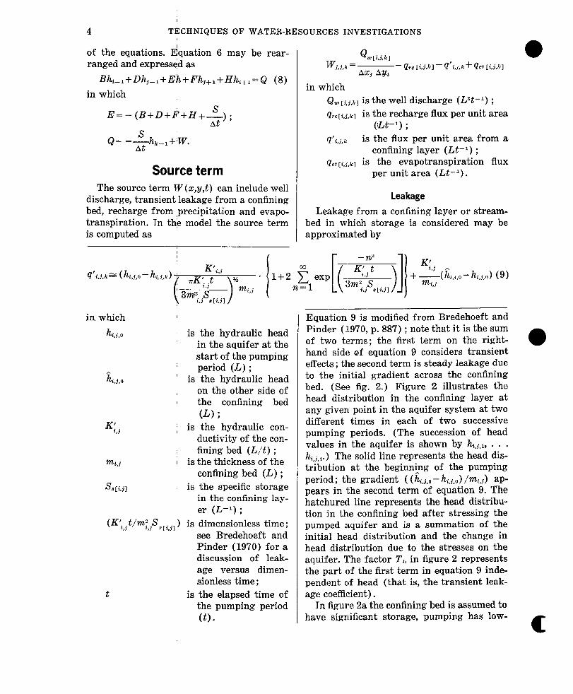
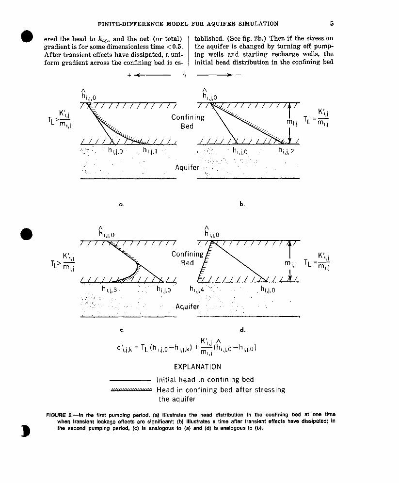
-- Equa.tion 9 is modified from Bredehoeft and Pinder (119’70, p. 887) ; note that it is the sum of two terms ; the first term on the right- 0 hand side of equation 9 considers transient effects ; the second term is steady leakage due to the initial gradient across the confining bed. (See fig. 2.) Figure 2 illustrates the head distribution in the confining layer at any given point in the aquifer system at two different times in each of two successive pumping periods. (The succession of head values in the aquifer is shown by ht,j,l, . . . hi,j,4.) The solid line represents the head dis- tribution at the beginning of the pumping period ; the gradient ( ( hi,i,o - hd,j,o) /mi,j) ap- pears, in ,the second term of equation 9. The hatchmred line represents the head distribu- tion in the confining bed after stressing the pumped aquifer and is a summation of the initial head distribution and the change in head distribution due to the stresses on the aquifer. The factor TL in figure 2 represents the part of the first term in equation 9 inde- pendent of head (that is, the transient leak- age coefficient).
In figure 2a the confining bed is assumed to have significant storage, pumping has low-
c
FINITE-DIFFERENCE MODEL FOR AQUIFER SIMULATION 5
0 ered the head to Iz~,~,~ and the net (or total) tablished. (See fig. 2b.) Then if the stress on gradient is for some dimensionless time <0.5. the aquifer is changed by turning off pump- After transient effects have dissipated, a uni- ing wells and starting recharge wells, the form gradient across the confining bed is es- initial head distribution in the confining bed
t-
6,,,,0 /By///////////
h --
A h f,l,O
a. b.
C. d.
q’,,j,k = TL th ,,j,O-h,,,,k) + K’,,j A ,I(hi,j,O-hi,j,O)
,
EXPLANATION
Initial head in confining bed m Head in confining bed after stressing
the aquifer
FIGURE 2.-In the first pumping period, (a) illustrates the head distribution in the confining bed at one time when transient leakage effects are significant; (b) illustrates a time after transient effects have dissipated: In the second pumping period, (c) is analogous to (a) and (d) is analogous to (b).
6 TECHNIQUES OF WATER-RESOURCES INVESTIGATIONS
for the new conditions is shown in figure 2c and is equal to the Anal distribution for the first pumping period! The net head distribu- tion in figure 2c is agected by storage in the confining bed and isifor some dimensionless time <0.5 (in the second pumping period). After storage effects have dissipated, the net gradient is shown in figure 2d.
For a simulation of several pumping peri- ods, the program assumes that transient leak- age effects from previous pumping periods have dissipated. This is accomplished at the start of each pumping period by initializing hi,i,O to the head at the end of the previous pumping period and/ setting t (and thereby dimensionless time) ’ to zero (note that the parameter storing the cumulative simulation time is not affected) 1 The assumption is rea- sonable if dimensio less P time for previous pumping periods is at least 0.5 (Bredehoeft and Pinder, 1970, fig. 4) and can be checked by noting the value of dimensionless time printed in the outputifor the end of the previ- ous pumping period. If the assumption is not valid, the code will need to be modified to in- clude transient effects for one or more previ- ous pumping periods.
hili,ol
I a. I I --
4
Z I
In the model, equation 9 is used until di- mensi~onless time reaches 3 x 10 --3 ; otherwise, the equation
!fi,j,kfb (hi,0 - hi,j,k)
is used. Equation 10 is computationally more efficielnt for dimensionless times greater than about 3 x :LO-3.
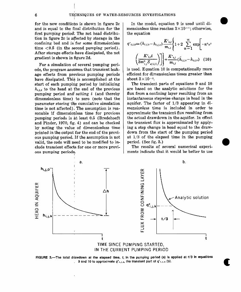
The transient parts of equations 9 and 10 are based on the analytic solutions for the flux from a confining layer resulting from an instantaneous stepwise change in head in the aquifer. The factor of l/3 appearing in di- mensionless time is included in order to approximate the transient flux resulting from the actual drawdown in the aquifer. In effect the transient flux is approximated by apply- ing a step change in head equal to the draw- down from the start of the pumping period at l/:3 of the elapsed time in the pumping period. (See fig. 3.)
The results of several numerical experi- ments indicate that it would be better to use
b.
solution
TIMIE SINCE PUMPING STARTED, IN THE CURRENT PUMPING PERIOD
FIGURE 3.-The total diawdown at the elapsed time, t, in the pumping period (a) is applied at t/3 in equations , 9 and 10 to approximate 9’,.,,r, the transient part of Q’w,~ (b).
c
FINITE-DIFFERENCE MODEL FOR AQUIFER SIMULATION 7
j¶ = 0.021
Hantush’s solution
1 o-3 10-Z K’t/m2Ss
10-l
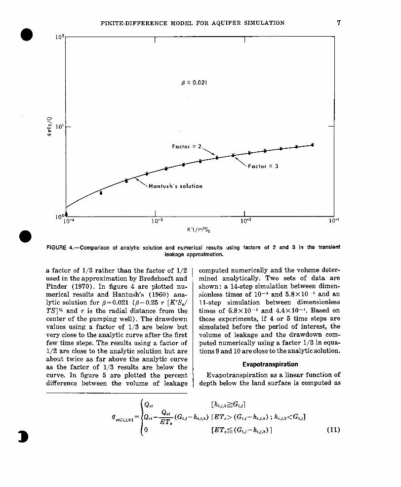
FIGURE 4.-Comparison of analytic solution and numerical results using factors of 2 and 3 in the transient leakage approximation.
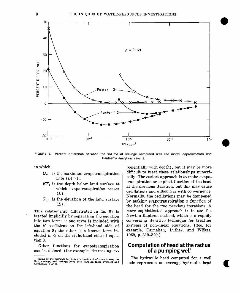
a factor of l/3 rather than the factor of l/2 used in the approximation by Bredehoeft and Pinder (1970). In figure 4 are plotted nu- merical results and Hantush’s (1960) ana- lytic solution for p= 0.021 (p = 0.25 r [K’S,/ TS]U and r is the radial distance from the center of the pumping well). The drawdown values using a factor of l/3 are below but very close to the analytic curve after the first few time steps. The results using a factor of l/2 are close to the analytic solution but are about twice as far above the analytic curve as the factor of l/3 results are below the curve. In figure 5 are plotted the percent difference between the volume of leakage
computed numerically and the volume deter- mined analytically. Two sets of data are shown: a 16step simulation between dimen- sionless times of lo+ and 5.8x10-* and an 11-step simulation between dimensionless times of 5.8~10-~ and 4.4X 10-l. Based on those experiments, if 4 or 5 time steps are simulated before the period of interest, the volume of leakage and the drawdown com- puted numerically using a factor l/3 in equa- tions 9 and 10 are close to the analytic solution.
Evapotranspiration
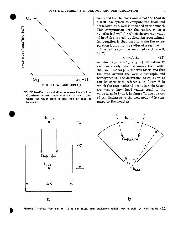
Evapotranspiration as a linear function of depth below the land surface is computed as
(11)
8
50
)C
0
-20 -
TECHNIQUES OF WATER-RESOURCES INVESTIGATIONS
/9 = 0.021
10-d 1 o-3 1 o-2
K’t/Ssm2 1 o-1 100
FIGURE 5.-Percent difference between the volume of leakage computed with the model approximation and Hantush’s analytical results.
in which
&et is the maximum evapotranspiration rate (U-l) ;
ET, is the depth below land surface at which evapotranspiration ceases WI ;
Gi,j is the elevation of the land surface W) *
This relationship (illustrated in fig. 6) is ’ treated implicitly by separating the equation
into two terms 1 : one term is included with the E coefficient on the left-hand side of equation 8 ; the other is a known term in- cluded in Q on the right-hand side of equa- tion 8.
ponentially with depth), but it may be more difficult to treat these relationships numeri- cally. The easiest approach is to make evapo- transpiration an explicit function of the head at the previous iteration, but this may cause oscillations and difficulties with convergence. Normally, the oscillations may be dampened by making evapotranspiration a function of the head for the two previous iterations. A more sophisticated approach is to use the Newton-Raphson method, which is a rapidly converging iterative technique for treating systems of non-linear equations. (See, for example, Carnahan, Luther, and Wilkes, 1969, p. 319329.)
Other functions for evapotranspiration Computation of head at the radius can be defined (for example, decreasing ex- of a pumping well
1 Some of the methods for implicit treatment of evapotranspira- tion. storage. and leakage have been adapted from Prick&t and Lonnsuist (1971).
The hydraulic head computed for a well node represents an average hydraulic head
FINITE-DIFFERENCE MODEL FOR AQUIFER SIMULATION 9
O- Gi,j Gi,j-ET,
DEPTH BELOW LAND SURFACE
FIGURE 6.-Evapotranspiration decreases linearly from Qet where the water table is at land surface to zero where the water table is less than or equal to GL,-ET..
Qw[i, j, k]/4
hi,j,k 0
-AX-
a
computed for the block and is not the head in a well. An option to compute the head and drawdown at a well is included in the model. This computation uses the radius, re, of a hypothetical well for which the average value of head for the cell applies. An approximat- ing equation is then used to make the extra- polation from re to the radius of a real well.
The radius re can be computed as (Prickett, 1967)
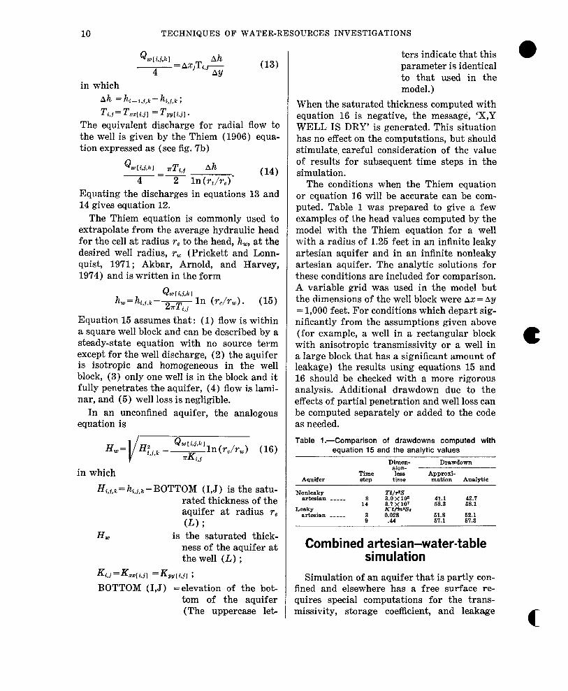
re = rJ4.81 (12) in which r1 =Axj= Ay, (fig. 7). Equation 12 assumes steady flow, no source term other than well discharge in the well block, and that the area around the well is isotropic and homogeneous. The derivation of equation 12 can be seen with reference to figure ‘7 in which the four nodes adjacent to node i,j are assumed to have head values equal to the value at node i - 1, j. In figure ‘7a one-quarter of the discharge to the well node i,j is com- puted by the model as
\/hi,i,k
b
3 FIGURE 7.-Flow from cell (i--l,/? to cell (Q)(a) and equivalent radial flow to well (i,n with radius r,(b).
10 TECHNIQUES OF WATER-RESOURCES INVESTIGATIONS
Q urli.Lkl ah 4
= Ax~T~,~--- (13) AY
ters indicate that this 0
in which Ah = hc-l,j,k- hi,j,k ; Ti,j= Tm[i,jl = Tg,[i,jl*
The equivalent discharge for radial flow to the well is given by the Thiem (1906) equa- tion expressed as (see fig. 7b)
Q ~1 ti,ikl T 77 i,j hh - =-- (14)
4 2 In (r&,)’ Equating the discharges in equations 13 and 14 gives equation 12.
The Thiem equation is commonly used to extrapolate from the average hydraulic head for the cell at radius re to the head, h,, at the desired well radius, rw (Prickett and Lonn- quist, 1971; Akbar, Arnold, and Harvey, 1974) and is written in the form
Qw~~.j.kI L = hi,j.k - 2nTj,j In (rehw) . (15)
Equation 15 assumes that: (1) flow is within a square well block and can be described by a steady-state equation with no source term except for the well discharge, (2) the aquifer is isotropic and homogeneous in the well block, (3) only one well is in the block and it fully penetrates the aquifer, (4) flow is lami- nar, and (5) well loss is negligible.
In an unconfined aquifer, the analogous equation is
I H,= V &J [ Likl Htjk --- , 3 J-G,
In (r&-d (16)
in which
Hi,j,k= hi,i,k - BOTTOM (1,J) is the satu- rated thickness of the aquifer at radius re (L) ;
HW is the saturated thick- ness of the aquifer at the well (L) ;
K4.j =Krnri.j, =Kgyli.jl ; BOTTOM (1,J) =elevation of the bot-
tom of the aquifer (The uppercase let-
parameter is identical to that used in the model.)
When the saturated thickness computed with equation 16 is negative, the message, ‘X,Y WELL IS DRY’ is generated. This situation has no effect on the computations, but should stimulate, careful consideration of the value of results for subsequent time steps in the simulation.
The conditions when the Thiem equation or equation 16 will be accurate can be com- puted. Table 1 was prepared to give a few examples of the head values computed by the model with the Thiem equation for a well with a radius of 1.25 feet in an infinite leaky artesian aquifer and in an infinite nonleaky artesian aquifer. The analytic solutions for these conditions are included for comparison. A variable grid was used in the model but the dimensions of the well block were Ax = Ay
= 1,000 feet. For conditions which depart sig- nificantly from the assumptions given above (for example, a well in a rectangular block with anisotropic transmissivity or a well in a large block that has a significant amount of leakage) the results using equations 15 and 16 should be checked with a more rigorous analysis. Additional drawdown due to the effects of partial penetration and well loss can be computed separately or added to the code as needed.
Table l.-Comparison of drawdowns computed with equation 15 and the analytic values
Aquifer Time BbP
Dimen- sion- less
time
Drawdown
Approxi- mation Analytic
Nonleaky artesian _____
Leaky srteman ---_-
TtP.9 3 41.1 42.7
14 ::70::::
68.3 68.1 Iww;,
i O:E8 E:! 62.1 67.3
Combined artesian-water-table simulation
Simulation of an aquifer that is partly con- fined and elsewhere has a free surface re- quires special computations for the trans- missivity, storage coefficient, and leakage
c
FINITE-DIFFERENCE MODEL FOR AQUIFER SIMULATION 11
term. The following paragraphs describe the computations required. Some of the methods of coding these procedures have been adapted from Prickett and Lonnquist (1971).
Transmissivity
The transmissivity is computed as the satu- rated thickness of the aquifer times the hy- draulic conductivity. This computation re- quires that the elevations of the top and bot- tom of the aquifer be specified. Where the aquifer crops out, the top of the aquifer is assigned a fictitious value greater than or equal to the elevation of the land surface.
Storage
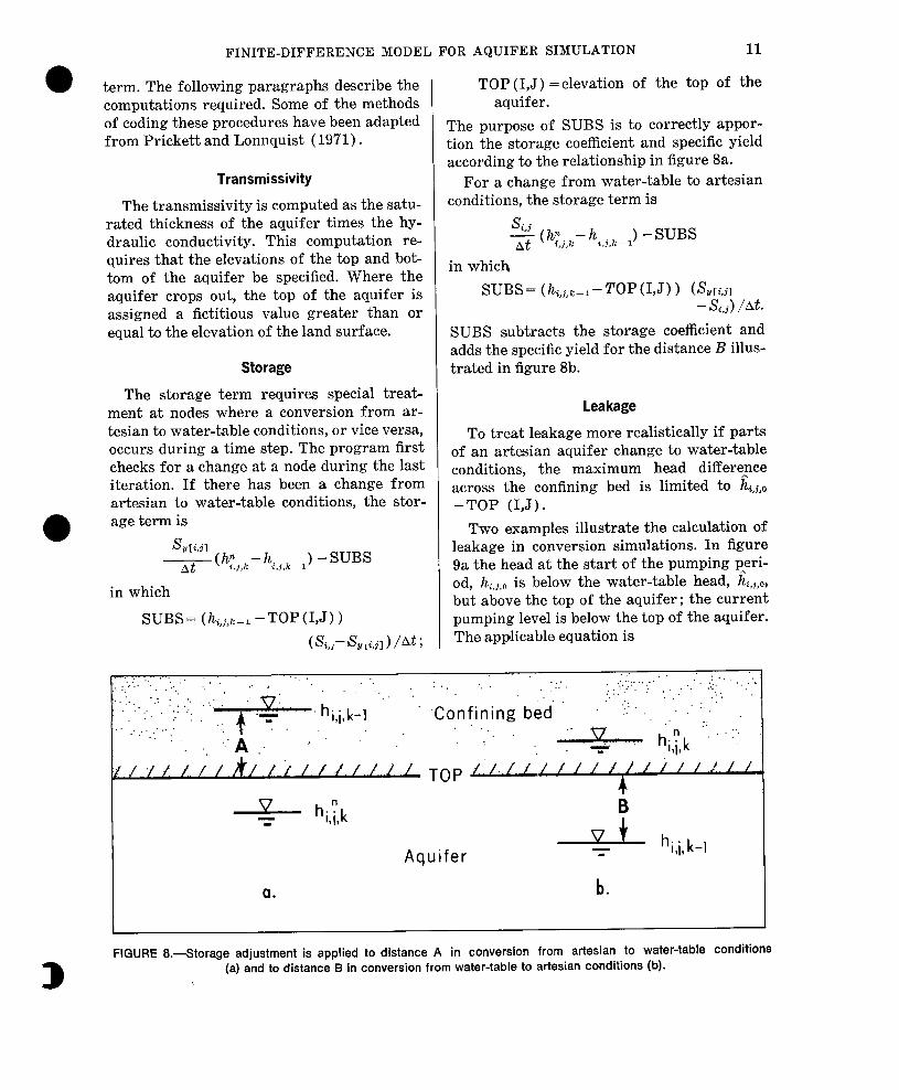
The storage term requires special treat- ment at nodes where a conversion from ar- tesian to water-table conditions, or vice versa, occurs during a time step. The program first checks for a change at a node during the last iteration. If there has been a change from artesian to water-table conditions, the stor- age term is
in which
SUBS = ( &i,~-l - TOP (I,J) 1
(&,j-Sy[i.jl 1 lAt ;
TOP (1,J) =elevation of the top of the aquifer.
The purpose of SUBS is to correctly appor- tion the storage coefficient and specific yield according to the relationship in figure 8a.
For a change from water-table to artesian conditions, the storage term is
g thy,,,,- hr,j,k--l) -SUBS
in which
SUBS= (hi,j,k-cTOP(I,J) 1 (Sy[i.j~ - L!&,~) /At.
SUBS subtra& the storage coefficient and adds the specific yield for the distance B illus- trated in figure 8b.
Leakage
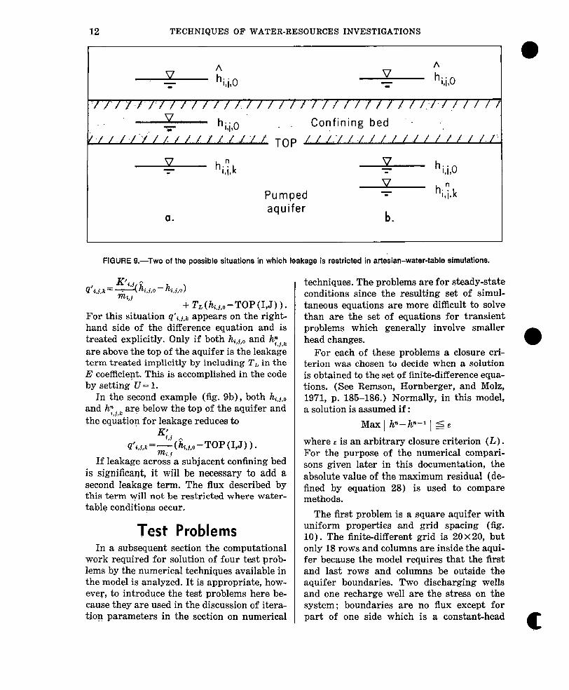
To treat leakage more realistically if parts of an artesian aquifer change to water-table conditions, the maximum head difference across the confining bed is limited to h,,j,,, -TOP (1,J).
Two examples illustrate the calculation of leakage in conversion simulations. In figure 9a the head at the start of the pumping peri- od, hi,i,o is below the water-table head, h,,,,, but above the top of the aquifer; the current pumping level is below the top of the aquifer. The applicable equation is
,. & - 1 1. / /.k/ / / / / f /./. / ./. TOP A.‘/. r’ / / i 1 J ./ / / 1 / / 1 1 /
& bilk 9 7
Aquifer - hi,i, k-1
a. b.
FIGURE 8.--Storage adjustment is applied to distance A in conversion from artesian to water-table conditions
D (a) and to distance B in conversion from water-table to artesian conditions (b).
12 TECHNIQUES OF WATER-RESOURCES INVESTIGATIONS
A V - hiiO I 1
FIGURE O.-Two of the possible situations in which leakage is restricted in artesian-water-table simulations.
“91 + TL t&,0 -TOP(I,J)).
For this situation q’c,j,k appears on the right- hand side of the difference equation and is treated explicitly. Only if both hi,j,o and h;,j,k are above the top of the aquifer is the leakage term treated implicitly by including TL in the E coefficient. This is accomplished in the code by setting U = 1.
In the second example (fig. 9b), both hi,j,o and h;,j,l, are below the top of the aquifer and the equation for leakage reduces to
K! . @i, j,k = - ,I’;&,,-TOP(I,J) 1.
If leakage across a subjacent confining bed is significant, it will be necessary to add a second leakage term. The flux described by this term will not be restricted where water- table conditions occur.
Test Problems In a subsequent section the computational
work required for solution of four test prob- lems by the numerical techniques available in the model is analyzed. It is appropriate, how- ever, to introduce the test problems here be- cause they are used in the discussion of itera- tion parameters in the section on numerical
techniques. The problems are for steady-state conditions since the resulting set of simul- taneous equations are more difficult to solve than are the set of equations for transient problems which generally involve smaller head changes. 0
For each of these problems a closure cri- terion was chosen to decide when a solution is obtained to the set of finite-difference equa- tions. (See Remson, Hornberger, and Molz, 19’71, p. 185-186.) Normally, in this model, a solution is assumed if:
Max 1 hn-hn-l 1 5 E
where E is an arbitrary closure criterion (L) . For the purpose of the numerical compari- sons given later in this documentation, the absolute value of the maximum residual (de fined by equation 28) is used to compare methods.
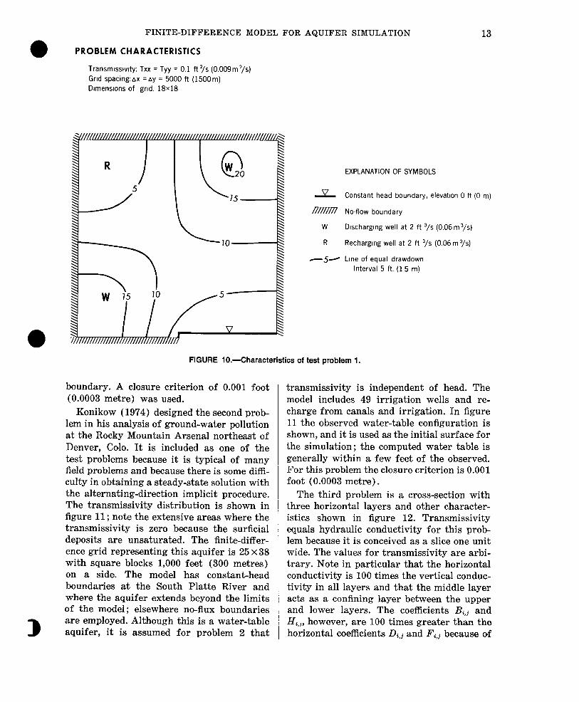
The first problem is a square aquifer with uniform properties and grid spacing (fig. 10). The finite-different grid is 20 x 20, but only 18 rows and columns are inside the aqui- fer because the model requires that the first and last rows and columns be outside the aquifer boundaries. Two discharging wells and one recharge well are the stress on the system ; boundaries are no flux except for part of one side which is a constant-head
c
FINITE-DIFFERENCE MODEL FOR AQUIFER SIMULATION 13
0 PROBLEM CHARACTERISTICS
Transmlsstvlty: Txx = Tyy = 0.1 ft ‘/s (0.009m ‘/s) Grad spacing:nx =ay = 5000 ft (1500m) Dlmenslons of gnd. 18x18
I T- 0 W 20
15-
EXPLANATION OF SYMBOLS
& Constant head boundary, elevation 0 ft (0 m)
m No-flow boundary
w Dlschargmg well at 2 ft “/s (0.06 m ‘/s)
R Recharging well at 2 ft “/s (0.06 m 3/s)
-5~ Lme of equal drawdown Interval 5 ft. (15 m)
FIGURE lO.-Characteristics of test problem 1.
boundary. A closure criterion of 0.001 foot (0.0003 metre) was used.
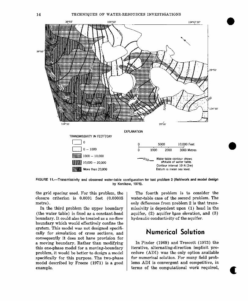
Konikow (1974) designed the second prob- lem in his analysis of ground-water pollution at the Rocky Mountain Arsenal northeast of Denver, Cdo. It is included as one of the test problems because it is typical of many field problems and because there is some diffi- culty in obtaining a steady-state solution with the alternating-direction implicit procedure. The transmissivity distribution is shown in figure 11; note the extensive areas where the transmissivity is zero because the surficial deposits are unsaturated. The finite-differ- ence grid representing this aquifer is 25 x38 with square blocks 1,000 feet (300 metres) on a side. The model has constantchead boundaries at the South Platte River and where the aquifer extends beyond the limits of the model; elsewhere no-flux boundaries are employed. Although this is a water-table aquifer, it is assumed for problem 2 that
transmissivity is independent of head. The model includes 49 irrigation wells and re- charge from canals and irrigation. In figure 11 the observed water-table configuration is shown, and it is used as the initial surface for the simulation; the computed water table is generally within a few feet of the observed. For this problem the closure criterion is 0.001 foot (0.0003 metre).
The third problem is a cross-section with three horizontal layers and other character- istics shown ,in figure 12. Transmissivity equals hydraulic conductivity for this prob- lem because it is conceived as a slice one unit wide. The values for transmissivity are arbi- trary. Note in particular that the horizontal conductivity is 100 times the vertical conduc- tivity in all layers and that the middle layer acts as a confining layer between the upper and lower layers. The coefficients Bi,j and Hi,,, however, are 100 times greater than the horizontal coefficients Di,j and Fi,j because of
14 TECHNIQUES OF WATER-RESOURCES INVESTIGATIONS
39055
TRANSMISSIVITY IN FEETZ/DAY EXPLANATION
no 0 5000 10,000 Feet
0 0 - 1000 0 ldoo 2ooo 3000 Metres
1000 - 10,000
10,000 - 20,000
More than 20,000
-~‘so, Water-table contour shows altitude of water table.
Contour interval 10 ft (3m) Datum IS mean sea level.
FIGURE Il.-Transmissivity and observed water-table configuration for test problem 2 (fieldwork and model design by Konikow, 1975).
the grid spacing used. For this problem, the closure criterion is 0.0001 feet (0.00003 metre) .
In the third problem the upper boundary (the water table) is fixed as a constant-head boundary. It could also be treated as a no-flow boundary which would effectively confine the system. This model was not designed specifi- cally for simulation of cross sections, and consequently it does not have provision for a moving boundary. Rather than modifying this one-phase model for a moving-boundary problem, it would be better to design a model specifically for this purpose. The two-phase model described by Freeze (1971) is a good example.
The fourth problem is to consider the water-table case of the second problem. The only difference from problem 2 is that trans- missivity is dependent upon (1) head in the aquifer, (2) aquifer base elevation, and (3) hydraulic conductivity of the aquifer.
Numerical Solution
In Pinder (1969) and Trescott (1973) the iterative, alternating-direction implicit pro- cedure (ADI) was the only option available for numerical solution. For many field prob- lems AD1 is convergent and competitive, in terms of the computational work required,
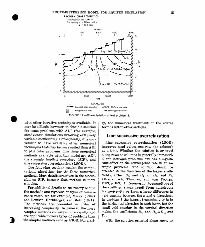
FINITE-DIFFERENCE MODEL FOR AQUIFER SIMULATION PROBLEM CHARACTERISTICS
Transmtsslwty Txx = 100 Tyy Grad spacmg AX = lOOOft (300117)
ay = 10 ft (3m)
METRES 0 1500 3000 4500 6000
1 Tyy = 10 ft (0.9m2/s)
0 0
0 6000 12000 18000
FEET
EXPLANATION
L Constant head boundary I$?%?%’ No-flow boundary
130- 135-- Equlpotentlal lines Vetilcal exaggeratm 83 1
FIGURE It.-Characteristics of test problem 3.
with other iterative techniques available. It may be difficult, however, to obtain a solution for some problems with AD1 (for example, steady-state simulations involving extremely variable coefficients). Consequently, it is con- venient to have available other numerical techniques that may be more suited than AD1 to particular problems. The three numerical methods available with this model are ADI, the strongly implicit procedure (SIP), and line successive overrelaxation (LSOR) .
The following sections outline the compu- tational algorithms for the three numerical methods. More details are given in the discus- sion on SIP, because that method is more complex.
For additional details on the theory behind the methods and rigorous analysis of conver- gence rates, see for example, Varga (1962) and Remson, Hornberger, and Molz (1971). The methods are presented in order of increasing complexity. In general, the more complex methods converge more rapidly and are applicable to more types of problems than the simpler methods such as LSOR. For clari-
15
ty, the numerical treatment of the source term is left to other sections.
Line successive overrelaxation Line successive overrelaxation (LSOR)
improves head values one row (or column) at a time. Whether the solution is oriented along rows or columns is generally immateri- al for isotropic problems but has a signifi- cant af%ct on the convergence rate in aniso- tropic problems. The solution should be oriented in the direction of the larger coeffi- cients, either &,! and H4,, or & and Fi,j (Breitenbach, Thurnau, and van Poollen, 1969, p. 159). Differences in the magnitude of the coefficients may result from anisotropic transmissivity or from a large difference in grid spacing between the x and y directions. In problem 3 the largest transmissivity is in the horizontal direction in each layer, but the small grid spacing in the vertical direction makes the coefficients & and Hi,,r* & and Fi,+
With the solution oriented along rows, an
16 TECHNIQUES OF WATER-RESOURCES INVESTIGATIONS
intermediate value is computed by the line Gauss-Seidel iteration formula,
Dh~~-l+Eh++Fh~+l=Qx,j=1,2, . . .,N, (17a)
in which
h+ is the intermediate head value at node (a ;
N, is the number of nodes in a row. Equation 17a can be expressed in matrix form as
=- A,h+ = &. (17b)
In order to reduce rounding errors, equa- tion 17b is put in residual form. (See Wein-
h= Ho
row 1
I
E, F, D, Es F,
D, Es 0 0 E, F,
D, Es F, D, E,
0
-
0
E, F, D, E, -F,
D, Es -
i!LO av 7(
I hl
t h4 L b
stein, Stone, and Kwan, 1969, p. 283, and Breitenbach, Thurnau, and van Poollen, 1969, p. 159.) This is accomplished by adding and subtracting &%-l to the right-hand side of equation 17b giving
A,~+=~,+Ax~n-l-Ax~~-l. (I7c) Rearrange equat,ion 17~ to read
A=,@ =&n--1 (17d)
in which ~+=~+.-~w;
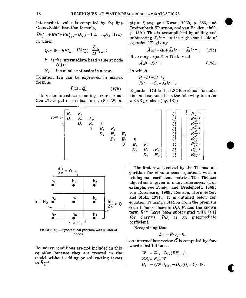
Equation 17d is the LSOR residual formula- tion and expanded has the following form for a 3x3 problem (fig. 13) :
hz 0
h5 0
h 0
h6 0
b
h=Ho9
FIGURE 13.-Hypothetical problem with 9 interior nodes.
Boundary conditions are not included in this equation because they are treated in the model without adding or subtracting terms to iy’.
The first row is solved by the Thomas al- gorithm for simultaneous equations with a tridiagonal coefficient matrix. The Thomas algorithm is given in many references. (For example, see Pinder and Bredehoeft, 1968; von Rosenberg, 1969 ; Remson, Hornberger, and Molz, 1971.) It is outlined below for equation 17 using notation from the program code (The coefficients D,.E,F, and the known term p-l have been subscripted with [i,j] for clarity). BE, is an intermediate coefficient.
Recognizing that
D,, = K,N,= 0, an intermediate vector C? is computed by for- ward substitution as
W = ELI-Di,j(BEj-d, BE, = F<,j,/ W Gj = (Rn-lii,jl - Di,j (G,-1) ) /W. c
FINITE-DIFFERENCE MODEL FOR AQUIFER SIMULATION 17
0 The values of $ for row i are then computed by backward substitution as
4n approximate equation for J is 3’z~yz--1+E’i(~i+~‘i(~i+l
=R’i,i=1,2,. . .,N, (18)
n which where
since
The head values for row 1 are then com- puted by the equation
h;l=h;;l+cotfj,j=l,. . .,Na I I If o is 1, the solution is by the line Gauss-
Seidel formula, but convergence is slow in general. The convergence rate is improved significantly by “overrelaxation” with l<~ < 2. Discussion of the acceleration parameter is deferred until after the following section on two-dimensional correction.
Two-dimensional correction to LSOR
In certain problems, the rate of conver- gence of LSOR can be improved by applying a one-dimensional correction (1DC) proce- dure introduced by Watts (1971) or the ex- tended two-dimensional correction (2DC) method described by Aziz and Settari (1972). These methods remove the components of certain eigenvectors in the LSOR iteration matrix from the solution vector. If the eigen- values associated with these eigenvectors dominate the problem, particularly those in- cluding anisotropy, the convergence rate is greatly improved.
The 2DC method is applied after one or more LSOR iterations. The corrected head values are used as an improved starting point for the next iteration and the process is re- peated until convergence is achieved.
The two-dimensional correction for the head at (i,j) is defined as
h;;,k= htj,,+ai+ij, i= 1,. . .,N, j= 1,. . .,N,
in which
h;“,;.k is the corrected head at iteration n; ffi is the correction for row i ; h A is the correction for column j. N, is the number of nodes in a column.
H’t = - 8Hs,j ; j
An approximate equation for ,? is D’j~i--1+E’g~~+F~j~~$1=:R’i,j =1,2,. . .,N,
(19) in which
D’j= - ZDc,j; 21
E’j=X(D,,~+Fc,t+S.~ ; i At
Equations 18 and 19 are derived with the following equations
flR;;=O, i=1,2,. . .,N,
,and
i$lRy;=O, j=:l,2,. . .,N,
which force the sum of residuals for each row and each column to zero when the vector Em* is substituted into equation 8. Aziz and Set- tari (1972) give the exact equations for z and g but point out that equations 18 and 19 are good approximations and, in practice, are easier to solve. For example, equation 19, which used alone is Watts’ 1DC method, is written ‘in matrix form as
18 TECHNIQUES OF WATER-RESOURCES INVESTIGATIONS
for the problem in figure 13. Equation 18 has an analogous form and both are easily solved by the Thomas algorithm.
Note that Cu and 2 in the model are zero for those rows and columns in which one or more_ constant-head nodes are located. If Cu and fi were not zero it would not be possible to maintain a constant value at the appropriate nodes. As Watts (1973) points out, therefore, the pro’cedure is most useful in simulations dominated by no-flow boundaries. For those simulations in which 2DC is useful, it is gen- erally better to apply the corrections after several rather than after each LSOR iterac tion. After experimenting with a few prob- lems, we have found it practical to apply 2DC after every 5 LSOR iterations.
LSOR acceleration parameter
The optimum value of o for maximum rate of convergence lies between 1 and 2 and is commonly between 1.6 and 1.9. If only one or two runs will be made on a problem, it is probably best to choose an o based on experi- ence. If. many runs will be made, it will be worthwhile to use an o close to the optimum value. For simple problems O,Bt can be com- put,ed as explained, for example, by Remson, Hornberger, and Molz (19’71, p. 188-199) us- ing the equation
2
w= I++p(G) (20)
in which
p(G) is the spectral radius (dominant eigen- value) of the Gauss-Seidel iteration matrix. For typical field problems it is possible to use equation 20 to estimate uopt in an iterative process if 2DC is not used. In the first simu- lation of the problem, set o= 1.0 and allow at least 100 iterations. In applying this method
to problems 1, 2, and 3 it took 25 iterations to arrive at mOpt for problem 2, but about 100 iterations to obtain WOpt for problem 1 and 3. Obviously this method may involve a lot of computational effort to obtain w,,~~. More effi- cient methods using equation 20 have been devised to update o during the iteration proc- ess. For example, Breitenbach, Thurnau, and van Poollen (1969) use a modified form of Varga’s (1962) “power method,” Carre’s (1961) method is described by Remson, Hornberger, and Molz (1971, p. 199-203)) and Cooley (1974) has a simple method for improving o for transient problems.
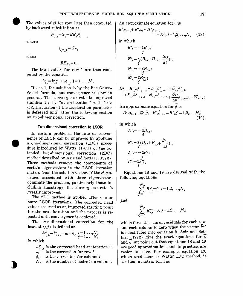
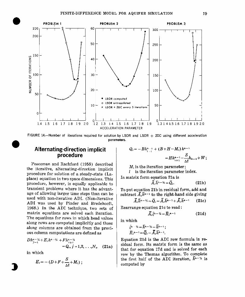
Figure 14 illustrates the rate of conver- gence of LSOR and LSOR+ 2DC for test problems 1, 2, and 3 using different accelera- tion parameters chosen by trial and error. The values exceeding 100 iterations for prob- lem 1 were estimated by using a plot, which is nearly a straight line, of the absolute value of the log of the maximum residual (defined by equation 28) versus the number of itera- tions. This plot was extrapolated to the value of maximum residual that corresponded roughly to the closure criterion chosen for the problem. The same procedure was used on problem 3 for values exceeding 200 iterations.
For problem 1 the optimum acceleration parameter is 1.87 for LSOR. Two-dimension- al correction significantly improves the con- vergence rate of LSOR for this problem with an optimum acceleration parameter of 1.7. In problem 2, 2DC had no effect on the rate of convergence of LSOR because of the numer- ous constant-head nodes in the problem. Con- sequently, the optimum acceleration parame- ter is 1.6 with or without the application of 2DC. In problem 3, with LSOR oriented across the bedding, Wopt is 1.88 for LSOR and about 1.70 for LSOR + 2DC. Note in problems 1 and 3 that finding Wept for LSOR is more critical than with LSOR+ 2DC. LSOR is poorly suited for problem 4 because too many nodes drop out in the iteration process if 1<0<2. Satisfactory results for problem 4 at the expense of slow convergence are ob- tained if 0 = 0.5 (See fig. 23.)
FINITE-DIFFERENCE MODEL FOR AQUIFER SIMULATION 19
0
PROBFFM 1 PROBLEM 2
I I I I I
60
50
40
30
20
10
0 1.4 1.5 16 1 7 18 19 2.0 2 1.3 14 1.5 1.6 1.7 18 .9 .3 14 1.5 1.6 1.7 18 1.9 2.0
ACCELERATION PARAMETER
l LSOR computed
o LSOR extrapolated
X LSOR + 2DC every 5 iteration!
I I I I I I
I
250
I-
O-
PpOBLEM 3
I I I I I I
Alternating-direction implicit procedure
Peaceman and Rachford (1955) described the iterative, alternating-direction implicit procedure for solution of a steady-state (La- place) equation in two space dimensions. This procedure, however, is equally applicable to transient problems where it has the advant- age of allowing larger time steps than can be used with non-iterative ADI. (Non-iterative AD1 was used by Pinder and Bredehoeft, 1968.) In the AD1 technique, two sets of matrix equations are solved each iteration. The equations for row,s in which head values along rows are computed implicitly and those along columns are obtained from the previ- ous column computations are defined as
Dh;I;h + E,.h”- % + Fh-f” =Q,,j=1,2,. . .,N, (21a)
in which
E,= - (D+F+;t+Mr) ;
FIGURE 14.-Number of iterations required for solution by LSOR and LSOR + 2DC using different acceleration parameters.
Qr= -Bhy~"_-,' + (B+H-A&)h"+'
-f&n-'- shx-l+ W; ‘+l At
M1 is the iteration parameter ; 1 is the iteration parameter index.
In matrix form equation 21.a is ~Jp-% = QT. @lb)
To put equation 21b in residual form, add and subtract A&+-l to the right-hand side giving
~~~*-~=a-~~~~-l+A=,~~-l (21c)
Rearrange equation 21~ to read : A=,p-n =j&n-1 GW
in which F”-‘/z=j+,L~n-1; &n-1=(&A=,+.
Equation 21d is the AD1 row formula in re- sidual form. Its matrix form is the same as that for equation 17d and is solved for each row by the Thomas algorithm. To complete the first half of the AD1 iteration, Em-n is computed by
20 TECHNIQUES OF WATER-RESOURCES INVESTIGATIONS
The equations in which head values along columns are considered implicitly and those along rows explicitly are written as : Bhin_l+E,h”+Hh~+I=&,,i=1,2,. . .,N, (22a)
in which
E,= - (B+H+;+il&) ;
&,= -Dh;y;h + (D+F-M,)hn-‘h
-Fhyy -;h,-,+ 74’.
Equation 22a in matrix form is z,iP= &. Wb)
By adding and subtracting ~&-~ to the right-hand side of equation 22b, it can be put in the residual form
&+~,n-$4; WC) in which
P =j+-j+M. j&n-M q&~&M.
Equation 22~ is solved for each column by the Thomas algorithm, and the vector @ for each row is obtained by the equation
j&j+%+f.
A set of iteration parameters is computed by the equation
M,=w, (B+D+F+H) in which ,,, ranges between a minimum de- fined by
Min x2 1 wmin= (over grid) 2p
?+ TM/ [t.j~ (Ax,)’ ’ T,, [i,:~ (4-h) ’
2
G 1 (23a)
u 1+ T z.n :z,j~ (W) ’ T uu to1 (Ax,)’
and a maximum given by
%lax = I 1 IT,,=T,,l; 2 [T,,>>T,, or T,,>>T,,l.
The set of parameters are spaced in a geo- metric sequence given by
w+1=yw Wb)
in which
ln Y
= In (%d%xia) I _ (23~) L-l
L =the number of iteration parame- ters used.
The iteration parameters starting with wmilr are cycled until convergence is achieved.
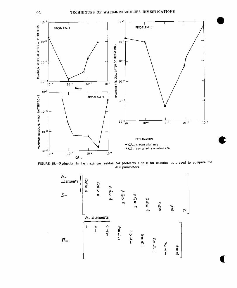
Equation 23a is based on a von Neuman error analysis of the normalized flow equa- tions. (See, for example, Weinstein, Stone, and Kwan, 1969.) It will compute the opti- mum CO,in only for simple problems. For gen- eral problems %lin computed by equation 23a may or may not be close to the optimum %in for the problem. This is illustrated in figure 15 in which the rate of reduction in the maxi- mum residual for arbitrarily chosen mini- mum parameters is compared with that for wnin computed with equation 23a. Ten param- eters were used in problems 1 and 2, and four parameters were used in problem 3. The lines on figure 15 are meant to show the general trend only. The convergence rate using the best qnir, in figure 15 is nearly the same as that computed with equation 23a for prob- lem 1, but there is a significant difference in 0
rates for problems 2 and 3. (See figs. 21 and 22. )
The other factor that may be critical in de- termining the rate of convergence using AD1 is the number of parameters. In general, the number of parameters is chosen as 5 if %ml - wmm is about two orders of magnitude ; if wmax -timin is three or more orders of magni- tude, 7 or more parameters are chosen.
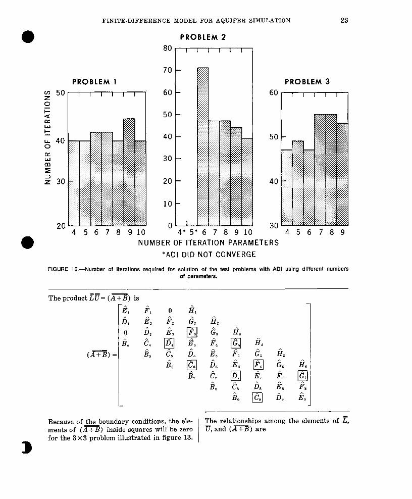
For the test problems, the number of itera- tion parameters were varied from 4 to 10 (fig. 16). The minimum parameter was cal- culated by equation 23a ; the maximum pa- rameter was 1 for problems 1 and 2 and was 2 for problem 3. The number of parameters had a relatively small effect in determining the rate of convergence for problems 1 and 3. For problem 2, however, the computations do not converge using 4 or 5 parameters. Prob- lem 2 can be solved with AD1 using 6 to 10 parameters with 10 parameters giving the most rapid convergence. AD1 did not give satisfactory solutions for problem 4 (an ex-
c
FINITE-DIFFERENCE MODEL FOR AQUIFER SIMULATION 21
cessive number of nodes always drop out of the solution) and, consequently, no results for problem 4 are shown in figure 16.
steady state should be achieved within a reasonable number of time steps with rapid convergence at each time step.
Strongly implicit procedure
When difficulties occur with AD1 in steady- state simulations, rather than experimenting with the critical minimum parameter or the number of parameters, it may be worthwhile to make the simulation a transient problem. In effect, S/At is used as an additional itera- tion parameter. If the storage coefficient is not made too large or the time step too small, ) XL=&
The set of equations (corresponding to equation 8) for the 3 x 3 problem in figure 13 may be expressed in matrix form as
(24)
L
Direct solution of equation 24 by Gaussian elimination usually requires more work and
0 computer storage than it,erative methods for problems of practical size because A’ decom- poses into a lower triangular matrix with non-zero elements from B to E in each row and an upper triangular matrix with non- zero elements from E to H in each row. All of these intermediate coefficients must be computed during Gaussian elimination, and the coefficients in the upper triangular ma- trix must be saved for backward substitution.
To reduce the computation time and stor- age requirements of direct Gaussian elimina- tion, Stone (1968) developed an iterative method using approximate factorization. In this approach a modifying matrix B is added - to A’ formi’ng (A + B) so that equation 24 becomes
(A+B)K=Q+EE. (25)
(A-) can be made close to x but can be factored in2 the product of a lower triangu- lar matrix L and an upper triangular matrix r, each of which has no more than three non- zero elements in each row, regardless of the size of N, and N,. Therefore, if the right- hand side of equation 25 is known, simple
recursion formulas can be derived, resulting in a considerable savings in computer time and storage. This leads to the iteration scheme --
(A+B)Iz”=~+B@-~. (26) In order to transform equation 26 into a residual form, K&l is subtracted from both sides giving --
(A+B)k=&’ (27) in which
P ,~n-~n-1. p-1 = Q- ~j&l. (2~)
The iterative scheme defined by equation 26 or 2’7 is closer to direct methods of solution (more implicit) than AD1 (hence the term strongly implicit procedure or SIP). The SIP algorithm requires (1) relationships among - the elements of z, g and (A + B) defined by rules of matrix multiplication for the equation
,? v’= (AT), and (2) relationships among the elements of Kand (Ax).
E and g have the following form for a general 3 x 3 problem (much of the notation is adapted from Remson, Hornberger, and Molz, 1971) ;
22 TECHNIQUES OF WATER-RESOURCES INVESTIGATIONS
10-g I I
2 0 PROBLEM 1
k
1o-4 10-3 10-2 1
0 ml,”
0-l
I I I PROBLEM 3
I I Ej PROBLEM 2
‘4 J
2 lo-‘0 -
. 1 O-“li
\ x
EXPLANATION
l O,,, chosen arbttrarlly
I I X &,, computed by equahon 23a
10-3 10-Z 10-I 0 ml”
FIGURE 15.-Reduction in the maximum residual for problems 1 to 3 for selected w,$, used to compute the ADI parameters.
N, Elements
I
N, Elements .
‘1 i1
0
:
F Y7 a9 pas ‘p” 9 Y9
c
FINITE-DIFFERENCE MODEL FOR AQUIFER SIMULATION 23
PROBLEM 1
--I
4 5 6 7 8 910
PROBLEM 2
8or--- 70 -
60 -
50 -
40 -
30 -
20 -
10 -
0’ 4* 5* 6 7 8 9 10
NUMBER OF ITERATION PARAMETERS *ADI DID NOT CONVERGE
PROBLEM 3
6ol----l
50
40
30 456789
FIGURE 16.-Number of iterations required for solution of the test problems with ADI using different numbers of parameters.
The product ~?a= (AT) is
(A+B)=
Because of the boundary conditions, the ele- The relationships among the elements of z, ments of (AT) inside squares will be zero
- g,and (A+B) are
B
for the 3x3 problem illustrated in figure 13.
24 TECHNIQUES OF WATER-RESOURCES INVESTIGATIONS
a =B (3W
a&-l & (30b)
P =fi (3Oc)
y+“~~-1+p6,-1 =JG WW
YS =@ We)
l&V-l =@ Wf)
Yrl =g wk) where the i and j subscripts refer to the loca- tion on the model grid, not in matrix (A-).
In order to use equations 30a-30g as the basis of a numerical technique for solving equation 24 efhciently by eliminationLrela- tionships between the elements of A and - (A+B) must be defined. One possibility is to let the elzments_correspond exactly and ig- nore the C and G diagonal in (AT). Stone (1968)) however, found that this could not be used as the basis of a rapidly convergent iterative procedure. Instead, he defined a family of modified matrices starting with 30b and 30f. -
Then the other elements of (A + B) can be defined as=equal to the corresponding ele; men+ in A plus a linear combination of C and G. For example
in which $I and & are constants depending on the problem being solved.
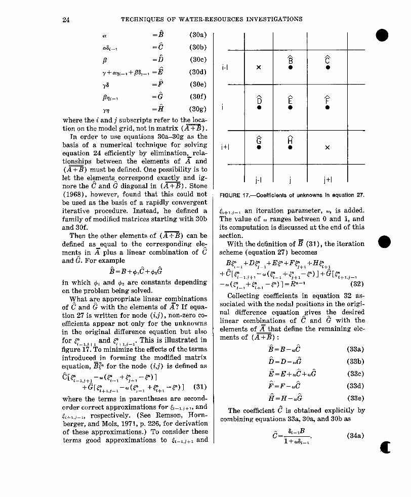
What aze appropriate linear cosbinations of C and G with the elements of A? If equa- tion 27 is written for node (i,j) , non-zero co- efficients appear not only for the unknowns in the original difference equation but also for qmlj+* and c+li--l. This is illustrated in figure 17. To minimize the effects of the terms introduced in forming the modified matrix equation, E@ for the node (i,j) is defined as
~[~-lj+l-d~-l+r;+l -P)l +&$+*j-l-w(ty-l +q+,-ml (31)
where the terms in parentheses are second- order correct approximations for &.l.i+l, and &+l,j-l, respectively. (See Remson, Horn- berger, and Molz, 1971, p. 226, for derivation of these approximations.) To consider these terms good approximations to &i-l,i+l and
i-l X
I B
i+l z
j-l
A 0 X
T j j+l
FIGURE 17.-Coefficients of unknowns in equation 27.
t D+l,j--l an iteration parameter, 0, is added. The value of o ranges between 0 and 1, and its computation is discussed at the end of this section.
With the definition of E (31)) the iteration 0 scheme (equation 27) becomes
Bq-l+D~-l+~$+J’~+, +Hq+, +erq, i+,-“(~~~~~~+,-F)l+~~~+, j-, -4q-1+q+1 -P)] =R”-’ ’ (3%
Collecting coefficients in equation 32 as- sociated with the nodal positions in the origi- nal difference equation gives the desired linear combinations of I? and 8 with the elements of x that define the remaining ele- - ments of (A+B) :
i?=B--wi? @a)
6=0-d (33b)
Jii=E+k+c12 (33c)
k=F-k W-W
ii=H-d We)
The coefficient 2 is obtained explicitly by combining equations 33a, 30a, and 30b as
& &-lB
l+osi-l’ @da)
a
FINITE-DIFFERENCE MODEL FOR AQUIFER SIMULATION 25
0
Finally combining equation 33b and equa- tions 3Oc and 30f gives
,A= V-ID 1+07]j-1.
Wb)
Equations 34, 33 and 30 (in that order) are the first part of the SIP algorithm.
Equation 28 written for node (i,j) is Rn-l=Q- (Bh;:;+Dh”-1 j-1
+Eh”-l+Fhy-;+Hhy-;).
As in the Thomas algorithm, the vector p is obtained by a process of forward and back- ward substitution. Combining equations 27 and 29 gives
~@=j+-l (35) Define an intermediate vector F by
@kp. (36) Then equation 35 becomes
~~=~?A~ (37) vn is first computed by forward substitution. This can be seen by writing equation 37 for node (i,j) :
0 aV;-, +/3V;~,+uVn=R”-’
or V”= (Rn-l-~V1_l-BV~_l)/Y.
The vector F may then be computed by back- ward substitution. Equation 36 for node (i,j) is
or P= V”-~~+, -‘1q+,.
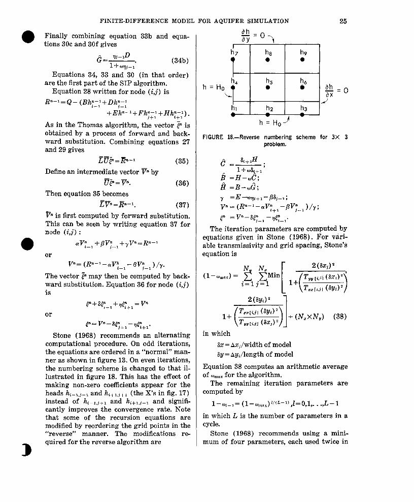
Stone (1968) recommends an alternating computational procedure. On odd iterations, the equations are ordered in a “normal” man- ner as shown in figure 13. On even iterations, the numbering scheme is changed to that il- lustrated in figure 18. This has the effect of making non-zero coefficients appear for the heads hi-1,j-1 and hi+l,j+l (the X’s in fig. 17) instead of hg-l,j+l and hi+l,j-l and signifi- cantly improves the convergence rate. Note that some of the recursion equations are modified by reordering the grid points in the “reverse” manner. The modifications re-
3
quired for the reverse algorithm are
FIGURE 18.-Reverse numbering scheme for 3X 3 problem.
Y =E -yYr]i+l-PSj--1;
vn = (R”-‘-aV;+, -P’;-, )/y;
p =vn-SC+, -7#- -
The iteration paramiteis are computed by equations given in Stone (1968 j. For vari- able transmissivity and grid spacing, Stone’s equation is
in which EX = AXj/width of model 6y = AyJength of model
Equation 38 computes an arithmetic average Of Oman for the algorithm.
The remaining iteration parameters are computed by
l- q+1= (l-wmax)~~(~-~),z=O,l,. . .,L-1
in which L is the number of parameters in a cycle.
Stone (1968) recommends using a mini- mum of four parameters, each used twice in
26 TECHNIQUES OF WATER-RESOURCES INVESTIGATIONS
succession, starting with the largest first. Weinstein, Stone, and Kwan (1969)) how- ever, indicate that it is not necessary to start with the largest parameter first or to repeat them.
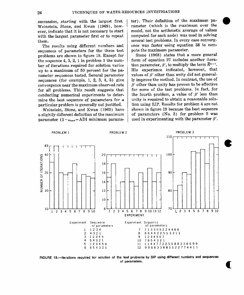
The results using different numbers and sequences of parameters for the three test problems are shown in figure 19. Except for the sequence 4, 3, 2, 1 in problem 1 the num- ber of iterations required for solution varies up to a maximum of 50 percent for the pa- rameter sequences tested. Several parameter sequences (for example, 1, 2, 3, 4, 5) give convergence near the maximum observed rate for all problems. This result suggests that conducting numerical experiments to deter- mine the best sequence of parameters for a particular problem is generally not justified.
Weinstein, Stone, and Kwan (1969) have a slightly different definition of the maximum parameter (1 - wII1.= = AD1 minimum parame-
PROBLEM 1
- 5 6
~ 7 8 91
ter). Their definition of the maximum pa- rameter (which is the maximum over the model, not the arithmetic average of values computed for each node) was used in solving several test problems. In every case converg- ence was faster using equation 38 to com- pute the maximum parameter.
Stone (1968) states that a more general form of equation 27 includes another itera- tion parameter, p’, to multiply the term En-l. His experience indicated, however, that values of p’ other than unity did not general- ly improve the method. In contrast, the use of /3’ other than unity has proven to be effective for some of the test problems. In fact, for the fourth problem, a value of p’ less than unity is required to obtain a reasonable solu- tion using SIP. Results for problem 4 are not shown in figure 19 because the best sequence of parameters (No. 3) for problem 2 was used in experimenting with the parameter p’.
PROBLEM 2
110
18
16
8 r I
Experiment Sequence of parameters
1 1234 2 4321 3 12345 4 54321 5 123456 6 654321
i iii, 3 4 5 6 7
90
80
PROBLEM 3
IIIIIlIIIl
EXPERIMENT
Experiment Sequence of parameters
7 113355224466 8 664422553311 9 1234567
10 7654321 11 114477225588336699 12 996633885522774411
7 8 9 10
FIGURE 19.4terations required for solution of the test problems by SIP using different numbers and sequences of parameters.
c
FINITE-DIFFERENCE MODEL FOR AQUIFER SIMULATION 27
Comparison of Numerical Results
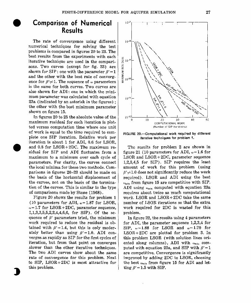
The rate of convergence using different numerical tech’niques for solving the test problems is compared in figures 20 to 23. The best results from the experiments with each iterative technique are used in the compari- sons. Two curves (except for fig. 23) are shown for SIP : one with the parameter ,R’= 1 and the other with the best rate of converg- ence for p’#l. The sequence of w parameters is the same for both curves. Two curves are also shown for ADI: one in which the mini- mum parameter was calculated with equation 23a (indicated by an asterisk in the figures) ; the other with the best minimum parameter shown on figure 15.
In figures 20 to 23 the absolute value of the maximum residual for each iteration is plot- ted versus computation time where one unit of work is equal to the time required to com- plete one SIP iteration. Relative work per iteration is about 1 for ADI, 0.6 for LSOR, and 0.8 for LSOR+2DC. The maximum reb sidual for SIP and AD1 fluctuates from a maximum to a minimum over each cycle of parameters. For clarity, the curves connect the local minima for these two methods. Com- parisons in figures 20-23 should be made on the basis of the horizontal displacement of the curves, not on the basis of the termina- tion of the curves. This is similar to the type of comparisons made by Stone (1968).
Figure 20 shows the results for problem 1 (10 parameters for ADI, O= 1.87 for LSOR, o = 1.7 for LSOR + 2DC, parameter sequence, 1,1,3,3 5 5 2 2 4 4 6 6 for SIP). Of the se- 99,99,,,, quence of p’ parameters tried, the minimum work required to reduce the residual is ob- tained with p’ = 1.4, but this is only moder- ately better than using p/=1.0. ADI con- verges as rapidly as SIP for the first cycles of iteration, but from that point on converges slower than the other iterative techniques. The two AD1 curves show about the same rate of convergence for this problem. Next to SIP, LSOR+ZDC is most attractive for
D this problem.
1 o-7 I I I I
0 10 20 30 40 50 COMPUTATIONAL WORK
(Number of SIP Iterataons)
FIGURE PO.-Computational work required by different iterative techniques for problem 1.
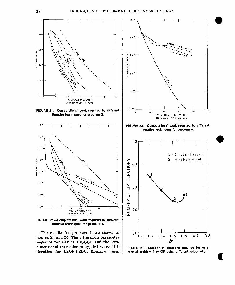
The results for problem 2 are shown in figure 21 (10 parameters for ADI, O= 1.6 for LSOR and LSOR + 2DC, parameter sequence 1,2,3,4,5 for SIP). SIP requires the least amount of work for this problem (using p’#l.O does not significantly reduce the work required). LSOR and AD1 using the best omi,, from figure 15 are competitive with SIP. AD1 using q,,in computed with equation 23a requires about twice as much computational work. LSOR and LSOR+2DC take the same number of LSOR iterations so that the extra work required for 2DC is wasted for this problem,
In figure 22, the results using 4 parameters for ADI, the parameter sequence 1,2,3,4 for SIP, o= 1.88 for LSOR and w=1.70 for LSOR+2DC are plotted for problem 3. In this problem LSOR (with solution lines ori- ented along columns), AD1 with *in com- puted with equation 23a, and SIP with p’= 1 are competitive. Convergence is significantly improved by adding 2DC to LSOR, choosing the best omin from figure 15 for AD1 and let- ting p’ = 1.5 with SIP.
28 TECHNIQUES OF WATER-RESOURCES INVESTIGATIONS
\ I I
10 I5 20
COMP”TATlONAL WORK (Number Of SIP Iterations)
FIGURE 21 .-Computational work required by different iterative techniques for problem 2.
FIGURE 22.-Computational work required by different iterative techniques for problem 3.
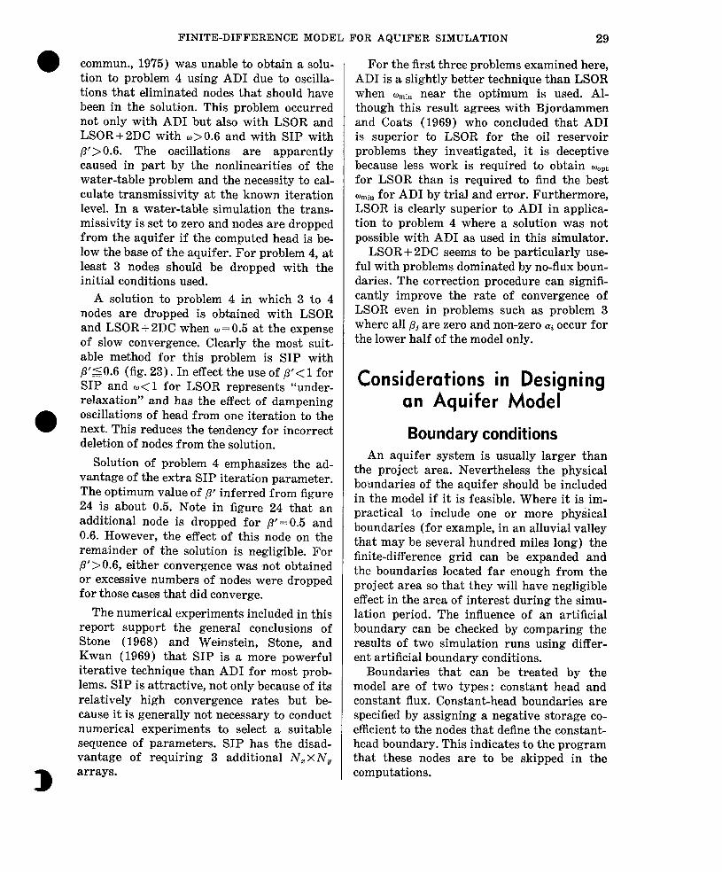
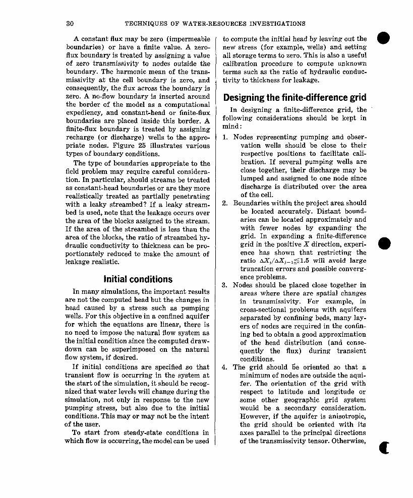
The results for problem 4 are shown in figures 23 and 24. The o iteration parameter sequence for SIP is 1,2,3,4,5, and the two- dimensional correction is applied every fifth iteratinn for LSOR+ 2DC. Konikow (oral
u 10 20 30 40 50
COMPUTATIONAL WORK (Number of SIP Iteratms)
FIGURE 23.-Computational work required by dlfferent iterative techniques for problem 4.
50
l-
/- 10 I b. 2 0.3 0.4 0.5 0.6 0.7 0.8
P’
I I I I
1 - 3 nodes dropped 2 - 4 nodes dropped
1
-lJ 1
2 2
I I I
FIGURE 24.-Number of iterations required for solu- tion of problem 4 by SIP using different values of P’.
FINITE-DIFFERENCE MODEL FOR AQUIFER SIMULATION 29
0
commun., 1975) was unable to obtain a solu- tion to problem 4 using AD1 due to oscilla- tions that eliminated nodes that should have been in the solution. This problem occurred not only with AD1 but also with LSOR and LSOR+ 2DC with ~>0.6 and with SIP with p’~O.6. The oscillations are apparently caused in part by the nonlinearities of the water-table problem and the necessity to cal- culate transmissivity at the known iteration level. In a water-table simulation the trans- missivity is set to zero and nodes are dropped from the aquifer if the computed head is bet low the base of the aquifer. For problem 4, at least 3 nodes should be dropped with the initial conditions used.
A solution to problem 4 in which 3 to 4 nodes are dropped is obtained with LSOR and LSOR + 2DC when w= 0.5 at the expense of slow convergence. Clearly the most suit- able method for this problem is SIP with p’90.6 (fig. 23). In effect the use of p’<l for SIP and 0<1 for LSOR represents “under- relaxation” and has the effect of dampening oscillations of head from one iteration to the next. This reduces the tendency for incorrect delet,ion of nodes from the solution.
Solution of problem 4 emphasizes the ad- vantage of the extra SIP iteration parameter. The optimum value of p’ inferred from figure 24 is about 0.5. Note in figure 24 that an addit,ional node is dropped for p’=O.5 and 0.6. However, the effect of this node on the remainder of the solution is negligible. For p’>O.6, either convergence was not obtained or excessive numbers of nodes were dropped for those cases that did converge.
The numerical experiments included in this report support the general conclusions of Stone (1968) and Weinstein, Stone, and Kwan (1969) that SIP is a more powerful iterative technique than AD1 for most prob- lems. SIP is attractive, not only because of its relatively high convergence rates but be- cause it is generally not necessary to conduct numerical experiments to select a suitable sequence of parameters. SIP has the disad- vantage of requiring 3 additional N,X N,
B arrays.
For the first three problems examined here, AD1 is a slightly better technique than LSOR when “mill near the optimum is used. Al- though this result agrees with Bjordammen and Coats (1969) who concluded that AD1 is superior to LSOR for the oil reservoir problems they investigated, it is deceptive because less work is required to obtain mopt for LSOR than is required to find the best umin for AD1 by trial and error. Furthermore, LSOR is clearly superior to AD1 in applica- tion to problem 4 where a solution was not possible with AD1 as used in this simulator.
LSOR + 2DC seems to be particularly use- ful with problems dominated by no-flux boun- daries. The correction procedure can signifi- cantly improve the rate of convergence of LSOR even in problems such as problem 3 where all pj are zero and non-zero (Y~ occur for the lower half of the model only.
Considerations in Designing on Aquifer Model
Boundary conditions An aquifer system is usually larger than
the project area. Nevertheless the physical boundaries of the aquifer should be included in the model if it is feasible. Where it is im- practical to include one or more phy&al boundaries (for example, in an alluvial valley that may be several hundred miles long) the finite-difference grid can be expanded and the boundaries located far enough from the project area so that they will have negligible effect in the area of interest during the simu- lation period. The influence of an artificial boundary can be checked by comparing the results of two simulation runs using differ- ent artificial boundary conditions.
Boundaries that can be treated by the model are of two types: constant head and constant flux. Constant-head boundaries are specified by assigning a negative storage co- efficient to the nodes that define the constant- head boundary. This indicates to the program that these nodes are to be skipped in the computations.
30 TECHNIQUES OF WATER-RESOURCES INVESTIGATIONS
A constant flux may be zero (impermeable boundaries) or have a finite value. A zero- flux boundary is treated by assigning a value of zero transmissivity to nodes outside the boundary. The harmonic mean of the trans- missivity at the cell boundary is zero, and consequently, the flux across the boundary is zero. A no-flow boundary is inserted around the border of the model as a computational expediency, and constant-head or finite-flux boundaries are placed inside this border. A finite-flux boundary is treated by assigning recharge (or discharge) wells to the appro- priate nodes. Figure 25 illustrates various types of boundary conditions.
The type of boundaries appropriate to the field problem may require careful considera- tion. In particular, should streams be treated as constant-head boundaries or are they more realistically treated as partially penetrating with a leaky streambed? If a leaky stream- bed is used, note that the leakage occurs over the area of the blocks assigned to the stream. If the area of the streambed is less than the area of the blocks, the ratio of streambed hy- draulic conductivity to thickness can be pro- portionately reduced to make the amount of leakage realistic.
Initial conditions In many simulations, the important results
are not the computed head but the changes in head caused by a stress such as pumping wells. For this objective in a confined aquifer for which the equations are linear, there is no need to impose the natural flow system as the initial condition since the computed draw- down can be superimposed on the natural flow system, if desired.
If initial conditions are specified so that transient flow is occurring in the system at the start of the simulation, it should be recog- nized that water levels will change during the simulation, not only in response to the new pumping stress, but also due to the initial conditions. This may or may not be the intent of the user.
To start from steady-state conditions in which flow is occurring, the model can be used
to compute the initial head by leaving out the 0 new stress (for example, wells) and setting all storage terms to zero. This is also a useful calibration procedure to compute unknown terms such as the ratio of hydraulic conduc- tivity to thickness for leakage.
Designing the finite-difference grid In designing a finite-difference grid, the ~
following considerations should be kept in mind : 1. Nodes representing pumping and obser-
vation wells should be close to their respective positions to facilitate cali- bration. If several pumping wells are close together, their discharge may be lumped and assigned to one node since discharge is distributed over the area of the cell.
2. Boundaries within the project area should be located accurately. Distant bound- aries can be located approximately and with fewer nodes by expanding the grid. In expanding a finite-difference grid in the positive X direction, experi- ence has shown that restricting the
0
ratio AX,/AXj-1~~.5 will avoid large truncation errors and possible converg- ence problems.
3. Nodes should be placed close together in areas where there are spatial changes in transmissivity. For example, in cross-sectional problems with aquifers separated by confining beds, many lay- ers of nodes are required in the confin- ing bed to obtain a good approximation of the head distribution (and conse- quently the flux) during transient conditions.
4. The grid should be oriented so that a minimum of nodes are outside the aqui- fer. The orientation of the grid with respect to latitude and longitude or some other geographic grid system would be a secondary consideration. However, if the aquifer is anisotropic, the grid should be oriented with its axes parallel to the principal directions of the transmissivity tensor. Otherwise,
c
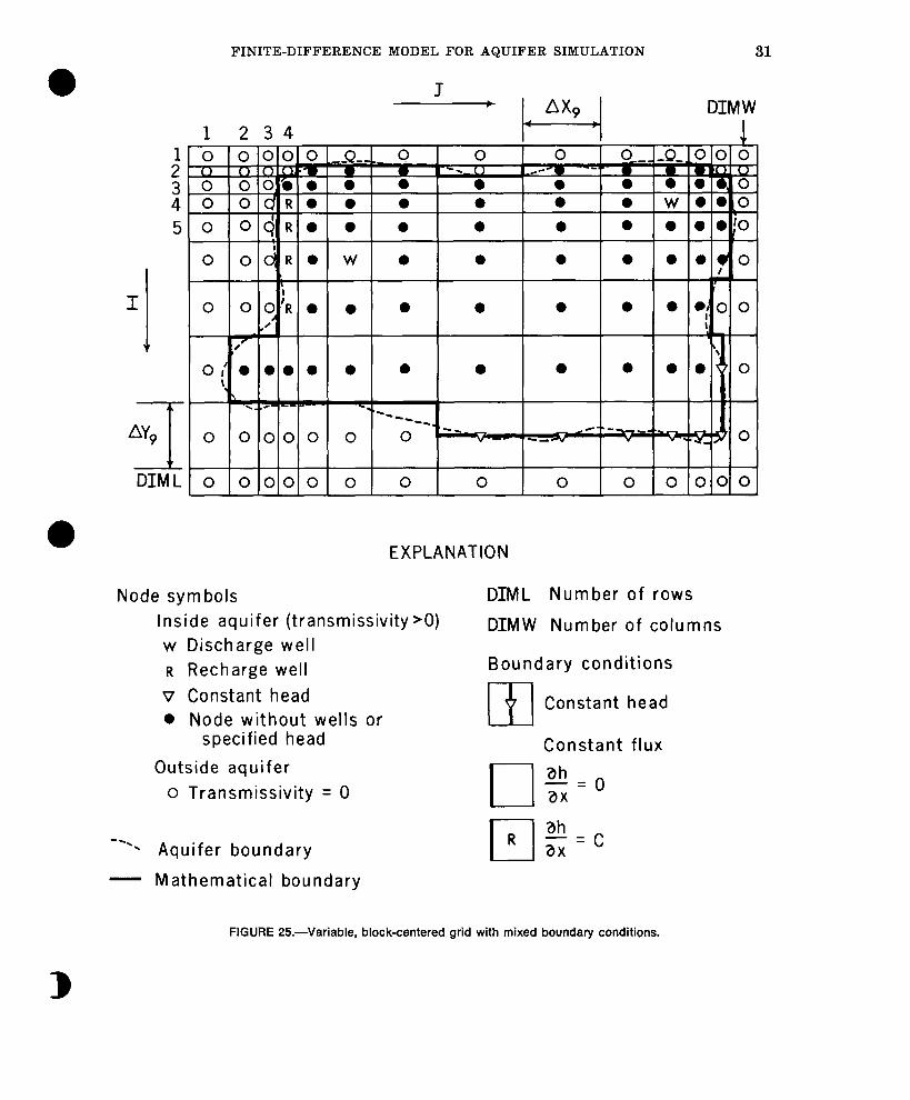
FINITE-DIFFERENCE MODEL FOR AQUIFER SIMULATION 31
I I
DIM L
DIMW
1 1 234
EXPLANATION
Node symbols Inside aquifer (transmissivity >O) w Discharge well R Recharge well v Constant head l Node without wells or
specified head
Outside aquifer o Transmissivity = 0
--. . Aquifer boundary
- Mathematical boundary
DIML Number of rows
DIMW Number of columns
Boundary conditions
Constant head
Constant flux
cl ah ax’
0
ah -- ax -C
FIGURE 25.-Variable, block-centered grid with mixed boundary conditions.
32 TECHNIQUES OF WATER-RESOURCES INVESTIGATIONS
the flow equation would include cross- product terms and the solution would be restricted to AD1 and LSOR because additional diagonals appear in the co- efficient matrix’ and SIP, in its usual form, cannot be used.
5. The rows should be numbered in the short dimension for the alphameric plot on the line printer or for plotting data with an X-Y plotter. On these plots, the X-direction is vertical and, for prac- tical purposes, this dimension is un- limited. The Y direction is across the page which limits this dimension to the maximum width of the page. (See fig. 26.)
6. The core requirements and computation time are proportional to the number of nodes representing the aquifer.
Selected References Akbar, A. M., and Arnold, M. D., and Harvey, 0. H.,
1974, Numerical simulation of individual wells in a field simulation model: Sot. Petrol. Eng. Jour., Aug. 1974, p. 315-320.
Aziz, K., and Settari, A., 1972, A new iterative meth- od for solving reservoir simulation equations: Jour. Canadian Petrol. Technology, Jan.-Mar. 1972, p. 62-68.
Bjordamman, J., and Coats, K. H., 1969, Compari- son of alternating-direction and successive over- relaxation techniques in simulation of reservoir fluid flow: Sot. Petrol. Eng. Jour., March, 1969, p. 47-58.
Bredehoeft, J. D., and Pinder, G. F., 1970, Digital analysis of area1 flow in multiaquifer ground- water systems : A quasi three-dimensional model : Water Resources Research, v. 6, no. 3, p. 883- 888.
Breitenbach, E. A., Thurnau, D. H., and van Poollen, H. K., 1969, Solution of the immiscible fluid flow simulation equations: Sot. Petrol. Eng. Jour., June 1969, p. 155-169.
Carnahan, B., Luther, H. A., and Wilkes, J. O., 1969, Applied numerical methods: New York, John Wiley and Sons, 604 p.
Car& B. A., 1961, The determination of the opti- mum accelerating factor for successive over-re- laxation: Comp. Jour., v. 4, p. 73-78.
Cooley, R. L., 1974, Finite element solutions for the ’ equations of groundwater flow: Desert Research
Institute Univ. Nevada, Tech. Report Series, H- W, Hydrology and Water Resources Pub. No. 18, 134 p.
Cosner, 0. J., and Horwich, E., 1974, Grid-coordinate 0 generation program: U.S. Geol. Survey open- - file report, 27 p.
Freeze, R. A., 1971, Three-dimensional, transient, saturated-unsaturated flow in a groundwater basin: Water Resources Research, v. 7, no. 2, p. 347-366.
Hantush, M. S., 1960, Modification of the theory of leaky aquifers: Jour. Geophys. Research, V. 65, no. 11, p. 3713-3725.
Konikow, L. F., 1974, Modeling mass transport in a shallow aquifer: Am. Geophys. Union Trans., v. 55, no. 4, p. 256.
1975, Hydrogeologic maps of the alluvial aquifer in and adjacent to the Rocky Mountain Arsenal, Colorado: U.S. Geol. Survey open-file report, 74-342.
Peaceman, D. W., and Rachford, H. H., Jr., 1955, The numerical solution of parabolic and elliptic dif- ferential equations: Sot. Indust. Appl. Math. Jour., v. 3, no. 1, p, 2841.
Pinder, G. F., 1969, An iterative digital model for aquifer evaluation: U.S. Geol. Survey open-file report, 43 p.
1970, A digital model for aquifer evaluation: U.S. Geol. Survey Tech. Water-Resources In- vestigations, Book 7, Chap. Cl, 18 p.
Pinder, G. F., and Bredehoeft, J. D., 1968, Applica- tion of a digital computer for aquifer evalua- tion: Water Resources Research, v. 4, no. 5, p. 1069-1093. l
Prickett, T. A., 1967, Designing pumped well char- acteristics into electric analog models: Ground Water, v. 5, no. 4, p. 38-46.
Prickett, T. A., and Lonnquist, C. G., 1971, Selected digital comuuter techniques for groundwater re- sources evaluation: Illinois State Water Survey Bull. 55, 62 p., Urbana.
Remson, I., Hornberger, G. M., and Molz, F. J., 1971, Numerical methods in subsurface hydrology: New York: Wiley-Interscience, 389 p.
Stone, H. K., 1968, Iterative solution of imulicit ap- proximations of multidimensional partial differ- ential equations: Sot. Indust. Appl. Math., Jour. Numer. Anal., v. 5, no. 3, p. 530-558.
Thiem, G., 1906, Hydrologische Methoden: Leipzig, Gebhardt, 56 p.
Trescott, P. C., 1973, Iterative digital model for aquifer evaluation: U.S. Geol. Survey open-file report, 18 p.
Varga, R. S., 1962, Matrix iterative analysis: New Jersey, Prentice-Hall, 322 p.
von Rosenberg, D. U., 1969. Methods for the numeri- cal solution of partial differential equations: New York, Elsevier, 128 p.
Watts, J. W., 1971, An iterative matrix solution method suitable for anisotropic problems: Sot. Petrol. Eng. Jour., March 1971, p. 47-51.
c
FINITE-DIFFERENCE MODEL FOR AQUIFER SIMULATION 33
0 - 1973, A method for improving line successive Weinstein, H. G., Stone, H. L., and Kwan, T. V.,
overrelaxation in anisotropic problems-a theore- 1969, Iterative procedure for solution of systems tical analysis: Sot. Petrol. Eng. Jour., April of parabolic and elliptic equations in three di- 1973, p. 105-118. mensions: Industrial and Eng. Chemistry Fun-
damentals, v. 8, no. 2, p. 281-287.

COMPUTER PROGRAM AND RELATED DATA
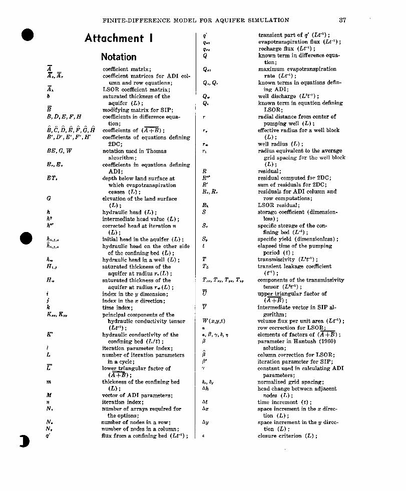
FINITE-DIFFERENCE MODEL FOR AQUIFER SIMULATION 37
Attachment I
AA b = B B,D,E,F,H
i,S,6,&fi,&!i B’,D’,E’,F’,H
BE, G, W
E.. E.
ET.
G
h hf h”’
h, H1.l
H,
i i k Kes, Ku,
K
L = L
m
M
“N.
N. N”
B 9’
Notation coefficient matrix; coefficient matrices for AD1 col-
umn and row equations; LSOR coefficient matrix; saturated thickness of the
aquifer (~5) ; modifying matrix for SIP; coefficients in difference equa-
tion; - coefficients of (A + B) ; coefficients of equations defining
2DC; notation used in Thomas
algorithm ; coefficients in equations defining
ADI; depth below land surface at
which evapotranspiration ceases (L) ;
elevation of the land surface (L) ;
hydraulic head (L) ; intermediate head value (L) ; corrected head at iteration n
G) ; initial head in the aquifer (L) ; hydraulic head on the other side
of the confining bed (L) ; hydraulic head in a well (L) ; saturated thickness of the
aquifer at radius re (L) ; saturated thickness of the
aquifer at radius rW (L) ; index in the y dimension; index in the 5 direction; time index; principal components of the
hydraulic conductivity tensor (LP) ;
hydraulic conductivity of the confining bed (L/t) ;
iteration parameter index; number of iteration parameters
in a cycle ; lower triangular factor of
(A-) ; thickness of the confining bed
(L) ; vector of AD1 parameters; iteration index ; number of arrays required for
the options; number of nodes in a row; number of nodes in a column ; flux from a confining bed (Lt-I) ;
9’ 90s 9re Q
&.I
Q., Q.
QO Q4
r
r.
T*
71
R R” R Rc, Rv
Ra s
s.
S”
T TL
Tz,, Tw, T,., TV, = u
v
a=, b Ah
At Ax
AY
transient part of 9’ (LP) ; evapotranspiration flux (Lt-‘) ; recharge flux (Lt-‘) ; known term in difference equa-
tion ; maximum evapotranspiration
rate (Lt-‘) ; known terms in equations defin-
ing ADI; well discharge (L’t”) ; known term in equation defining
LSOR; radial distance from center of
pumping well (L) ; effective radius for a well block
(L) ; well radius (L) ; radius equivalent to the! average
grid spacing for the well block (L) ;
residual ; residual computed for 2DC; sum of residuals for 2DC; residuals for AD1 column and
row computations ; LSOR residual; storage coefficient (dimension-
less) ; specific storage of the con-
fining bed (L-l) ; specific yield (dimensionless) ; elapsed time of the pumping
period (t) ; transmissivity (L’t-I) ; transient leakage coefficient
(t-9 ; components of the transmissivity
tensor (L’t-I) ; upper triangular factor of -
(A+B) ; intermediate vector in SIP al-
gorithm; volume flux per unit area (Lt-I) ; row correction for LSOR;_ elements of factors of (A+B) ; parameter in Hantush (1960)
solution ; column correction for LSOR; iteration parameter for SIP; constant used in calculating AD1
parameters ; normalized grid spacing; head change between adjacent
nodes (L) ; time increment (t) ; space increment in the x direc-
tion (L) ; space increment in the v direc-
tion (L) ; closure criterion (L) ;
38 TECHNIQUES OF WATER-RESOURCES INVESTIGATIONS
vector of change in head over an iteration;
spectral radius of Gauss-Seidel iteration matrix;
constants in definition of co- - efficients of (A+B) ;
acceleration parameter; iteration parameter; maximum iteration parameter; minimum iteration parameter; optimum acceleration parameter.
printed on the first page of the output as ‘WORDS OF VECTOR Y USED=XXXX’.
a
In the second part of the main program, the location of the initial addresses of the arrays are passed to the subroutines. (See table 3 for details.) The variables in table 3 defining the dimensions of the arrays are defined in Attachment VI; the first four arrays and XII are double precision.
Attachment II, Computer Program
Main program The first function of the main program is
to dimension the arrays for the field problem being simulated. The algorithm allocates storage space reserved in a vector, Y. Some arrays are required for every simulation ; others are needed only if certain options are specified. The information needed to allocate space to the arrays is contained in the Group I data cards which are read by the main program (see Attachment III).
Once the model is compiled, it does not need to be recompiled for a new field prob- lem unless (1) the logic is changed or (2) the vector Y is not dimensioned large enough for the new problem. The minimum dimen- sion of the vector Y (YDIM) can be com- puted by
The last part of the main program controls the sequence of computations illustrated by the generalized flow chart (Appendix V) . In the flow chart, the routines are lettered in se- quence starting with the main program. Entry points for the routines are numbered in sequence along the left side of the chart. Exits from a routine are indicated by circles containing the entry point of the routine to which control passes. A break occurs in the flow chart following an unconditional exit. Variables used in the flow chart are defined in Attachment VI.
Subroutine DATAI
YDIMr(15+N,)iV,N, (39) in which N, is the total number of arrays required for the options (from table 2).
Equation 39 is approximate, but normally will give a value that is sufficient for the sim- ulation. The exact dimension required -is
Instructions for the preparation of the data deck are given in Attachment III. Data may 0 be input to the model in any consistent set of units in which second is the time unit. It is organized into four groups: Data in groups I and II are the simulation options and scalar parameters: group III cards are used to ini- tialize the arrays. These three groups are re- quired for each new simulation. Group IV contains data that varies with each new pumping period. The program permits chang- ing well discharge and the time parameters each pumping period, but the program can be modified to read other data (for example, recharge rate) with this set of cards.
Table P.-Number of arrays required for the optlons Time parameters
Number of Option arrays
Water Table ______________________ 3 Conversion1 -- _____ -_-__------___-- 1 Leakage -_____________--__________ 3 Evapotranspiration _____ -- ______ -___ 1 SIP --_-____-_____________________ 4
1 Conversion also requires the arrays for the water table option.
The time parameters include the initial time step, DELT; a multiplication factor for increasing the size of the time step, CDLT ; the number of time steps, NUMT; and the simulation period, TMAX. Since the rate of water-level decline decreases during a pump- ing period, the time step is increased by the factor CDLT each step (commonly 1.5). For
c
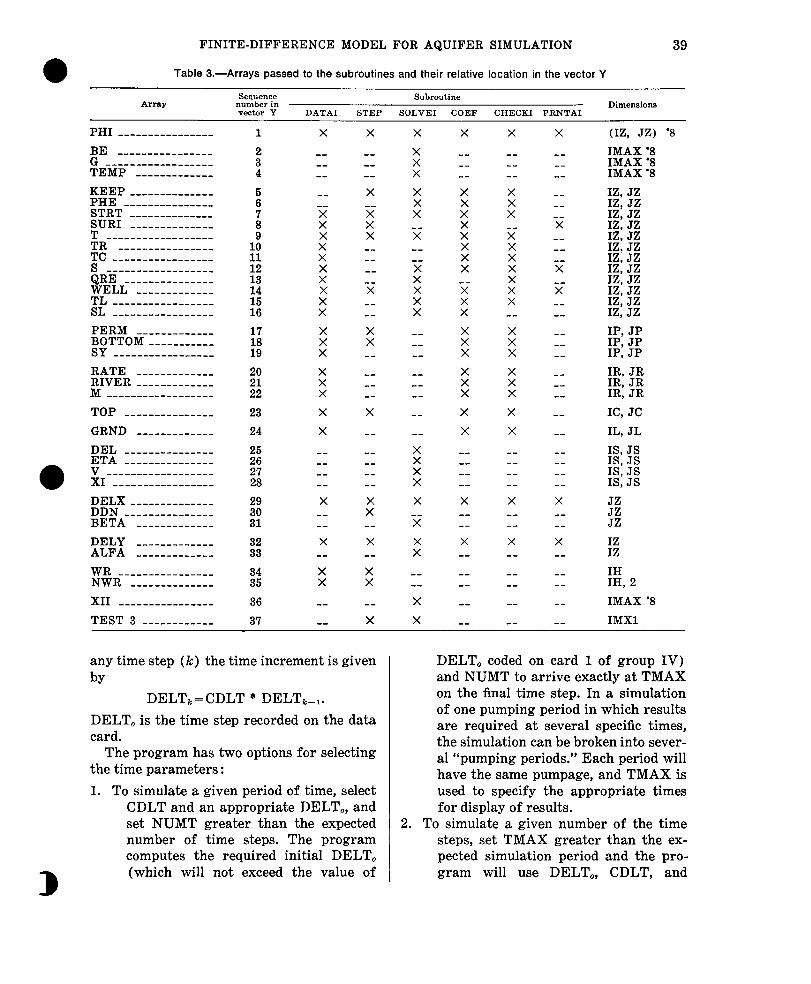
FINITE-DIFFERENCE MODEL FOR AQUIFER SIMULATION
Table 3.-Arrays passed to the subroutines and their relative location in the vector Y
39
Array Sesut?llce Subroutine
number in Dimensions vector Y DATA1 STEP SOLVE1 COEF CHECK1 PRNTAI
PHI ________________
KEEP ______________ PHE _______________ STRT ______________ $JRI ______________ I ------------------
TR ____-___________ TC _________________ s - - - - - - - - - - - - - - - - - - QRE ___ _____ _ ______ WELL _____________ TL _________________ SL ------------- ----
PERM _______ - _____ BOTTOM ___________ SY -------- --- -_-- __
RATE _____________ RIVER _____________ M -----___----______
TOP _______________
GRND _____________
DEL _______________ ETA _______________ v ------------------ XI - - - - - - - - - - - - - - -- -
DELX ______________ DDN _______________ BETA _____________
DELY _____________ ALFA _____________
WR _-______--__-___ NWR ______________
XII - -- - --- ----- ----
TEST 3 ____________
X
-- -- --
-- --
x” X
:: X X X
x”
X
x”
:: X
X
X
-- -- -- --
X -- --
X --
::
--
--
X
-- -- --
X -- X X X -- -- -- -- X -- --
X X --
-- -- --
X
--
-- -- -- --
X X --
X --
X X
--
X
X
X
::
X
x” -- X -- -- X X
:: X
-- -- --
-- -- --
--
--
::
::
X -- X
x”
-- --
X
X
X
-- -- --
X
x”
x” X
x” --
:: X
X X X
X
::
X
X
-- -- -- --
X -- --
X --
-- --
--
--
X
-- -- --
X
x” -- X
::
:: X X --
X
::
X X X
X
X
-- -- -- --
X -- --
X --
-- --
--
--
X
-- -- --
-- -- -- X -- -- -- X -- X -- --
-- -- --
-- -- --
--
--
-- -- -- --
X -- --
X --
-- --
--
--
(IZ, JZ) ‘8
IMAX ‘8 IMAX ‘8 IMAX ‘8
IZ, JZ IZ? JZ IZ, JZ IZ, JZ IZ. JZ IZ: JZ IZ. JZ IZ, JZ IZ, JZ IZ, JZ IZ, JZ IZ? JZ
IP, JP
E: ;pP
IR, JR IR, JR IR, JR
IC, JC
IL, JL
IS, JS IS, JS IS, JS IS, JS
;;
::
2, 2
IMAX l 8
IMXl
any time step (k) the time increment is given by
DELTr= CDLT * DELTk-,. DELT, is the time step recorded on the data card.
The program has two options for selecting the time parameters : 1. To simulate a given period of time, select
CDLT and an appropriate DELT,, and set NUMT greater than the expected number of time steps. The program computes the required initial DELT, (which will not exceed the value of
2.
DELT, coded on card 1 of group IV) and NUMT to arrive exactly at TMAX on the final time step. In a simulation of one pumping period in which results are required at several specific times, the simulation can be broken into sever- al “pumping periods.” Each period will have the same pumpage, and TMAX is used to specify the appropriate times for display of results.
To simulate a given number of the time steps, set TMAX greater than the ex- pected simulation period and the pro- gram will use DELT,, CDLT, and
40 TECHNIQUES OF WATER-RESOURCES INVESTIGATIONS
NUMT as specified on the time param- eter card.
To minimize the error due to approxima- tion of the time derivative, several time steps should be simulated before the first step at which results are displayed. This suggestion should be followed unless the system is nearly steady-state before the results are needed. In this case a one-step simulation may be satis- factory, but this approach should be checked by making one run as a multistep simulation so that the results can be compared.
For steady-state simulations, set the stor- age coefficient and (or) specific yield of the aquifer and the specific storage of the con- fining bed to zero. Compute for one time step of any length (for example, set TMAX= 1, NUMT=l, CDLT=l, DELT=24) and the program should iterate to a solution. The maximum permitted number of iterations (ITMAX) should be larger for steady-state than for transient simulations. If the calcu- lations do not converge to a solution within a reasonable number of iterations, it may be necessary to use a transient simulation for enough steps to attain steady state (see also the discussion of AD1 iteration parameters) or use another numerical technique.
Initialization
In addition to reading data and computing the time parameter, this routine initializes other arrays and scalar parameters. In par- ticular, note that the leakage coefficient, TL, will equal K'i,j/'m,j and can be computed once for the entire simulation if the specific stor- age of the confining bed is zero. The compu- tation of the steady leakage term, SL, and the division of well discharge by the area of the cell need to be done only once for each pumping period. At the beginning of each pumping period the starting head (STRT) and the simulation time (SUMP) used in computing transient leakage are initialized.
Subroutine STEP Subroutine STEP initializes variables for
a new time step, checks for steady-state con- ditions after a solution is obtained for thu
time step, and controls the printing and punching of results and the writing of results
0
on disk. If head values are punched at the end of the simulation or are written on disk, they can be used to extend the simulation or as input to plotting routines. (See the pro- gram by Cosner and Horwich, 1974.) Cur- rently, a general program is being written to display results in various forms on the line printer and plotters ; it is described in detail in another section of this report.
In the check for steady state during tran- sient simulations, the head change over a time step is computed. If the absolute value of change at all nodes is less than EROR, the message ‘STEADY STATE AT TIME STEP X’ is printed. The program then prints all desired output for the final time step (X) and proceeds to read data for the next pump- ing period, if any.
Maximum head change for each iteration
The printed results are explained in the section on theory and in the discussions of subroutines COEF, CHECKI, and PRNTAI or are self explanatory, except for the listing e of the absolute value of the maximum head change for each iteration. This information is useful if convergence is slow with AD1 or SIP because it may indicate that a slightly larger error criterion will give a satisfactory solution with considerably fewer iterations.
Subroutine SOLVE
The three SOLVE routines, SOLVEl, SOLVE& and SOLVE3 are, respectively, SIP, LSOR and ADI. They have been de- scribed in previous sections, but a few addi- tional comments are necessary.
In these routines and in subroutine COEF, the usual (I,J) notation has been replaced in favor of single-subscript notation. Less time is involved in finding the value of a variable with a single subscript than in finding the value of one with a double subscript and, as a consequence, computational efficiency is im- proved. The five variables used as subscripts in this notation are defined in Attachment VI.
c
FINITE-DIFFERENCE MODEL FOR AQUIFER SIMULATION 41
SIP iteration parameters
The algorithm in ITERl permits computa- tion of the iteration parameters in increasing or decreasing order and repeat of parameters depending on the initialization of the vector IORDER. Note that LENGTH is twice the number of different parameters and that the DATA statement that initializes IORDER assumes LENGTH = 10. Replace the DATA statement with a READ statement if addi- tional flexibility is desired in choosing the order of parameters without recompiling the subroutine.
Exceeding permitted iterations
If the permitted number of iterations for a time step is exceeded, the message ‘EX- CEEDED PERMITTED NUMBER OF ITERATIONS’ is printed. Following the message the mass balance, head matrix, etc., as specified in the options are printed for the final iteration. This information is useful in determining the cause of the nonconvergence.
0
Before terminating the run, the mass balance and head values will be punched if PUNC was specified in the options or written on disk if IDK2 was specified. With punched output or results on disk, the user has the option to extend the number of iterations if it appears that a solution can be obtained. If iterations are exceeded on the first time step, the head values saved (punched or written on disk) were computed in the last iteration. If iterations are exceeded on a subsequent time step, KT, the head values and mass-balance parameters saved are the results for time step KT-1.
Subroutine COEF Most of the calculations for coefficients
used in the solution of the numerical schemes are done in this routine. The more extensive computations except those described in the section on theory are discussed in the fol- lowing paragraphs.
Transient leakage coefficients
The algorithm for the transient parts of equations 9 and 10 is the same except for two
conditional statements that recompute PPT and DENOM if dimensionless time is in the range for applying equation 9. In performing the infinite summation, the code checks for the significance of additional terms, but in any case limits the summation to a maximum of 200 terms. The minimum and maximum values of dimensionless time, TMIN and TT, are retained and printed with the results for the time step so that the user will know whether or not transient leakage effects are significant.
Transmissivity as a function of head
The transmissivity for water-table or com- bined water-table-artesian aquifers is com- puted as a function of the saturated thick- ness of the aquifer. If a cell (except a cell with well discharge) goes dry, a message ‘NODE I, J GOES DRY’ is printed, the trans- missivity for the cell is set to zero, and the head is set to the initial surface (so that the location of the cell will show up in the out- put). No provision is made to permit the cell to resaturate in subsequent pumping periods because the additional code necessary to accommodate this special situation is not warranted in a general program.
When a cell with well discharge goes dry (that is, a hypothetical well with radius rR goes dry), the program terminates the com- putation with printed output, and, if speci- fied in the options, saves the results. Printed output is headed by ‘WELL I, J GOES DRY’ followed by drawdown when the well went dry. If results for the previous time step were not printed, drawdown and a mass balance (if specified in the program options) for the previous time step are printed. Finally, if specified in the options, mass-balance pa- rameters and head values for the previous time step are punched or written on disk so that the user has the option of continu- ing the simulation after modifying the well discharge.
TR and TC coefficients
The TR and TC arrays save values that are used repeatedly in the algorithm. They are computed once for artesian problems and
42 TECHNIQUES OF WATER-RESOURCES INVESTIGATIONS
each iteration for water-table and combined artesian-water-table simulations. TR (1,J) is the harmonic mean of T,, (1,J) /DELX (J) , T,,(I,J+l)/DELX(J+l); TC (1,J) is the harmonic mean of T,, (1,J) /DELY (I), T, (I+l,J)/DELY(I+l).
are plotted for each cell with the rightmost 0
Subroutine CHECKI
A mass balance is computed in this routine. The results are expressed in two ways: (1) as a cumulative volume of water from each source and each type of discharge and (2) as rates for the current time step.
In the cumulative mass balance, storage is treated as a source of water. Flow to and from constant-head boundaries is computed with Darcy’s law using the gradients from constant-head nodes to adjacent nodes inside the aquifer. Other computations in the al- gorithm are self explanatory.
The difference between the sum of sources and sum of discharges from the system is usually less than 1 percent. A larger error, however, does not necessarily mean that the results are poor; it may be due to lack of precision in calculating the mass balance. This has been observed, for example, if a leaky streambed is given a large K’/m ratio so that it is effectively a constant-head bound- ary. The leakage computation is inaccurate if the heed values at a stream node are identi- cal to 6 or ‘7 significant figures and they are stored as single precision variables.
To the right of the cumulative mass bal- ance are printed the flow rates for the cur- rent time step. They are self explanatory except for leakage. “Leakage from previous pumping period” is the leakage resulting from gradients across the confining bed at the start of the current pumping period. The “total” leakage is the sum of leakage due to the initial gradients plus leakage induced by head changes during the current pumping period.
Subroutine PRNTAI This routine prints a map of drawdown
and hydraulic head. Up to three characters
character as close to the location of the node as the printer will allow. An option to per- mit the printing of results at different scales in the x and y dimensions is useful for cross sections. This routine is useful for displaying results during calibration runs. More elegant graphical displays for final results are de- scribed in another section.
The user specifies XSCALE and YSCALE, the multiplication factors required to change from units used in the model to units used on the map; DINCH, the number of map units per inch; FACT1 and FACTB, the multiplica- tion factors for adjusting the values of draw- down and head to be plotted, respectively ; and MESUR, the name of the unit used on the map. As an example, assume that the length unit used in the model is feet, the map is to be scaled at 3 miles per inch and draw- down values at 1 foot increments and head values at 10 foot increments are to be plotted. Then XSCALE = YSCALE = 5280, DINCH=3, FACTl=l, FACTZ=O.l; and MESUR=MILES.
To print a map of maximum possible size, number the ‘rows in the short dimension to take advantage of the orientation of the map on the computer page where the X direction is vertical and, the Y direction horizontal. (See fig. 26.) The origin is the upper left- hand corner of the block for row 2, column 2. Orienting the map with the origin in the upper left-hand corner, the right and bottom sides of the map include the node locations for the second to last column and row, respec- tively. The border is located to the nearest inch outside these node locations and may or may not fall on the cell boundaries depending on the scaling. The map is automatically cen- tered on the page and is limited to a maxi- mum of 12 inches (300 mm) in the Y direc- tion. If the parameters for a map are speci- fied such that the Y dimension is more than 12 inches (300 mm) adjustments are auto- matically made to fit the map within this limit. A common mistake is to specify a value for Y scale that is less than 1.0. This gen- erates the message ‘NOTE: GENERALLY SCALE SHOULD BE > OR = 1.0,’ and a suit-
c
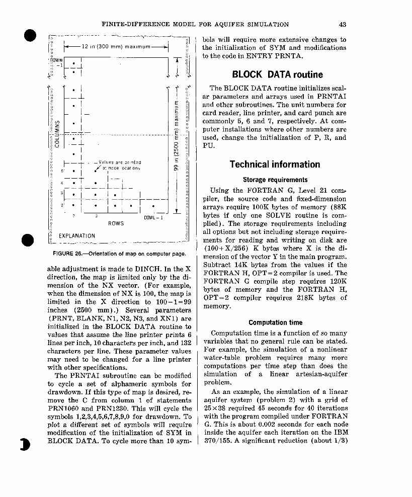
FINITE-DIFFERENCE MODEL FOR AQUIFER SIMULATION 43
DIML - 1
,” ROWS
FIGURE 26.-Orientation of map on computer page.
able adjustment is made to DINCH. In the X direction, the map is limited only by the di- mension of the NX vector. (For example, when the dimension of NX is 100, the map is limited in the X direction to lOO- 1=99 inches (2500 mm) .) Several parameters (PRNT, BLANK, Nl, N2, N3, and XNl) are initialized ,in the BLOCK DATA routine to values that assume the line printer prints 6 lines per inch, 10 characters per inch, and 132 characters per line. These parameter values may need to be changed for a line printer with other specifications.
The PRNTAI subroutine can be modified to cycle a set of alphameric symbols for drawdown. If this type of map is desired, re- move the C from column 1 of statements PRN1060 and PRN1230. This will cycle the symbols 12 3 4 5 6 ‘7 8 9 0 , , , , , 9 , t , for drawdown. To plot a different set of symbols will require modification of the initialization of SYM in BLOCK DATA. To cycle more than 10 sym-
bols will require more extensive changes to the initialization of SYM and modifications to the code in ENTRY PRNTA.
BLOCK DATA routine The BLOCK DATA routine initializes scal-
ar parameters and arrays used in PRNTAI and other subroutines. The unit numbers for card reader, line printer, and card punch are commonly 5, 6 and ‘7, respectively. At com- puter installations where other numbers are used, change the initialization of P, R, and PU.
Technical information
Storage requirements
Using the FORTRAN G, Level 21 corn piler, the source code and fixed-dimension arrays require 1OOK bytes of memory (88K bytes if only one SOLVE routine is com- plied). The storage requirements including all options but not including storage require- ments for reading and writing on disk are (100-1-X/256) K bytes where X is the di- mension of the vector Y in the main program. Subtract 14K bytes from the values if the FORTRAN H, OPT=2 compiler is used. The FORTRAN G compile step requires 120K bytes of memory and the FORTRAN H, OPT=2 compiler requires 218K bytes of memory.
Computation time
Computation time is a function of so many variables that no general rule can be stated. For example, the simulation of a nonlinear water-table problem requires many more computations per time step than does the simulation of a linear artesian-aquifer problem.
As an example, the simulation of a linear aquifer system (problem 2) with a grid of 25x38 required 45 seconds for 40 iterations with the program compiled under FORTRAN G. This is about 0.002 seconds for each node inside the aquifer each iteration on the IBM 370/155. A significant reduction (about l/3)
44 TECHNIQUES OF WATER-RESOURCES INVESTIGATIONS
in execution time can be achieved by using the FORTRAN H compiler which generates a more efficient code than the FORTRAN G compiler.
Further significant reductions in execu- tion time can be achieved if the model is de- signed for a specific problem. Problem 3, for example, does not require computation of leakage, storage, or evapotranspiration terms.
Use of disk fqcilifies for storage of array data and interim results
In an effort to expedite use of the program on remote terminals connected to the IBM 3’70/155, options are included to utilize disk storage facilities. These options enable stor- age and retrieval of array data (STRT, PERM, and so forth) and the saving of in- terim head values without punching them on cards.
Use of these options can be particularly beneficial at remote terminals with low speed data transmission or without punch output capability. Also, the type of read statements used afford more efficient data transmission from disk than from cards.
Storage of array data is accomplished via a direct access data set that is defined by a DEFINE FILE statement in the main pro- gram (card MAN0480) and by a DD state- ment in the JCL string used to execute the program. To establish the data set, the DE- FINE FILE statement and the DD statement must indicate the amount of space that is required. The DEFINE FILE statement takes the following form :
DEFINE FILE 2 (14,???,U,KKK) MAN0480
where ??? is the number of nodes for the problem being solved (DIMLxDIMW) . Pa- rameters U and KKK are indicators and do not vary.
The DD statement contains information, such as account number, that will be differ- ent for each user. Also, the first reference to the data set is somewhat different from sub- sequent references. To utilize one of the disk packs provided by the system (IBM 370/
155) for semipermanent storage of user data, the first reference to the data set will take the following general form if the FORTGCG procedure is used to compile and execute the program. //GO. FT02FOOl DD DSN =Azzzzzz.AZbbb.
cxxwwwww.aaaaaaaa, // UNIT = (I)NLINE,DISP = (NEW,
KEEP), // SPACE= (????,(14)),DCB=
(RECFM=F) where
zzzzzz
bbb
c
xx
are the first six digits of a nine digit account number;
are the last three digits of a nine digit account number ;
is the center code (same as column 3 on job card) ;
is the two digit organization code (same as columns 4 and 5 on job card) ;
wwwww is the four or five digit pro- gram number (same as the program number beginning in column 24 of the job card) ;
aaaaaaaa is any 1 to 8 character name used to designate the name of the data set;
???? is the number of bytes per record that are to be re- served and should be set equal to DIMLxDIMWx4.
The instructions for the DSN parameter are also given in the CCD users manual, chapter 5, pages 3 and 4. When this initial allocation is processed the system will indi- cate in the HASP system log, JCL string out- put, the volume on which the data set was established (for example, SYSOll or SYS015). Subsequent use of the data set must indicate this information by modifying the underlined parameters in the initial ref- erence to the data set. Thus the DD state- ment will read:
//G@ FTOZFOOl DD DSN = Azzzzzz.Azbbb. cxxwwwwwaaaaaaaa,
FINITE-DIFFERENCE MODEL FOR AQUIFER SIMULATION 45
0 // UNIT = (dNLINE, DISP = SHR,V@L - = SER = YYYYYY
where the DSN parameter is the same as the initial run and yyyyyy indicates the volume (for example, SYS015) on which the data set was established by the initial run. The individual data arrays that are to be stored and later retrieved from this data set are specified on the parameter card for each ar- ray. These specifications will be discussed completely in the section on Data Deck In- structions (Attachment III).
If use of this option is selected, space for buffers must be reserved via the REGION parameter on the EXEC card. The amount of space needed is approximately equal to two times the number of bytes per record (indicated in the SPACE parameter on the DD card defined above).
Interim results (head values, cumulative simulation time, and mass-balance parame- ters) can be punched on cards or can be stored and retrieved from data sets on disk in much the same manner as array data. Use
0 of storage on disk is initiated by parameters on the simulation options card. (See attach- ment III, card 3.)
Definition of the sequential data set on disk where the information will be stored is ac- complished by a DD statement in the JCL string used to execute the program. If one of the system disk packs is used to store the data set, the first reference to the data will be different from subsequent references as in the case of array data sets. The first refer- ence will take the following form if the FORTGCG procedure is used. //G@ FT04FOOl DD DSN = Azzzzzz.AZbbb.
rxxwwwwwaaaaaaaa, // UNIT = @NLINE, DISP = (NEW,
KEEP) ,SPACE = (TRK, (1,l) , RLSE) ,
// DCB= (RECFM=VBS,LRECL = dddd, BLKSIZE = eeee)
The DSN parameter is defined in the same manner as previously discussed for the direct access (array) data sets and : dddd-equals DIMLxDIMWx8 + 48 (56440)
B eeee-equals DIMLxDIMWx8 + 52 (56440)
If BLKSIZE (eeee) exceeds 6444, code 6444 for (eeee) and 6440 for (dddd) . Also, addi- tional core equal to about two times the value of BLKSIZE must be reserved for buffers via the REGION parameter on the EXEC card.
Once the initial reference to the data set has been successfully processed, the system will indicate (via the JCL printout) on what volume the data set has been established (for example, SYSOll or SYSO15) and, subse- quent references to the data set will appear as follows : //G@ FT4FOOl DD DSN = Azzzzzz.AZbbb.
cxxwwwww.aaaaaaaa,
// UNIT=@NLINE, V@L=SER= yyyyyy,DISP = SHR
where yyyyyy is the name of the disk pack (for example, SYSOll) that contains the data set and DSN is as previously described.
To destroy (erase) an array data set or an interim results data set, simply execute the following job. // EXEC PGM=IEFBR14 //X DD DSN = Azzzzzz.AZbbb.cxxwwwww.
aaaaaaaa, // UNIT = (dNLINE, V@L= SER = yyyyyy,
DISP = (@LD,DELETE)
Use of the disk facilities is illustrated in Appendix IV.
Graphical display package
A series of computer programs are cur- rently being written and assembled that will enable graphical display of results of com- puter models. Components of this graphical display package will include :
1. time-series plots of model results on the printer,
2. time-series plots on pen plotters (CAL- COMP),
3. contour maps of model results at selected time steps on the printer,
4. contour maps utilizing pen plotters, and 5. other graphical displays, such as perspec-
tive (three-dimensional) drawings.
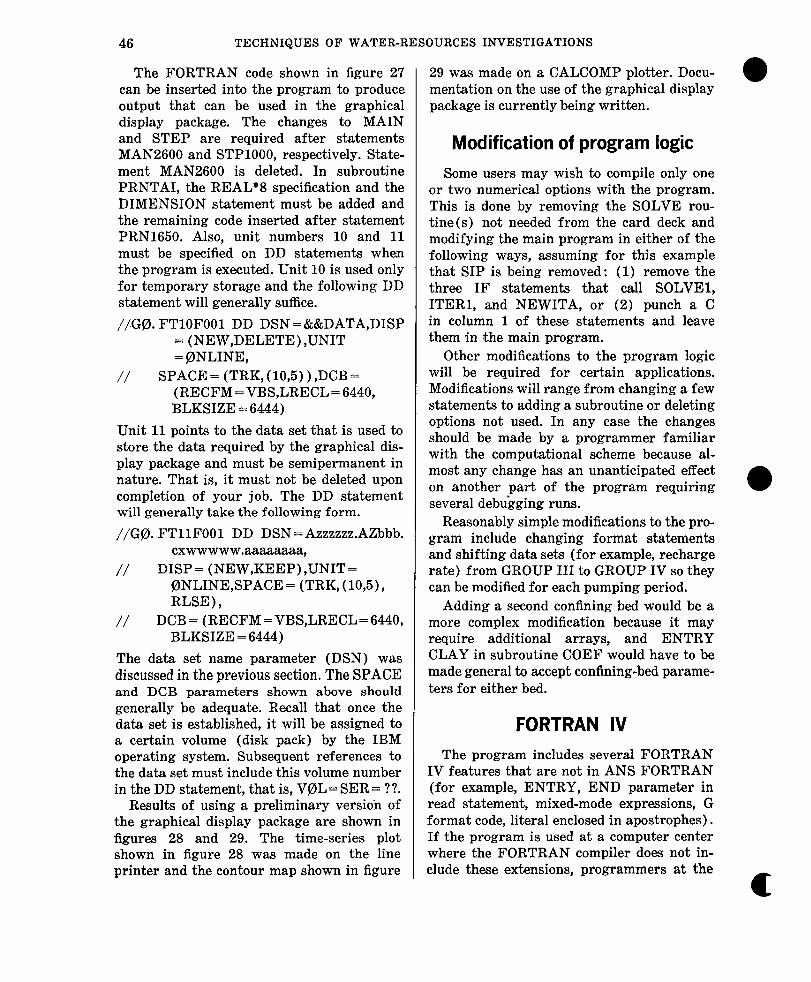
46 TECHNIQUES OF WATER-RESOURCES INVESTIGATIONS
The FORTRAN code shown in figure 27 can be inserted into the program to produce output that can be used in the graphical display package. The changes to MAIN and STEP are required after statements MAN2600 and STPlOOO, respectively. State- ment MAN2600 is deleted. In subroutine PRNTAI, the REAL*8 specification and the DIMENSION statement must be added and the remaining code inserted after statement PRN1650. Also, unit numbers 10 and 11 must be specified on DD statements when the program is executed. Unit 10 is used only for temporary storage and the following DD statement will generally suffice. //Go. FTlOFOOl DD DSN =&&DATA,DISP
= (NEW,DELETE) ,UNIT = ONLINE,
// SPACE = (TRK, (10,5) ) ,DCB = (RECFM=VBS,LRECL=6440, BLKSIZE = 6444)
Unit 11 points to the data set that is used to store the data required by the graphical dis- play package and must be semipermanent in nature. That is, it must not be deleted upon completion of your job. The DD statement will generally take the following form. //Ge). FTllFOOl DD DSN = Azzzzzz.AZbbb.
cxwwwww.aaaaaaaa, // DISP = (NEW,KEEP) ,UNIT =
gNLINE,SPACE = (TRK, (10,5), RLSE),
// DCB= (RECFM=VBS,LRECL=6440, BLKSIZE = 6444)
The data set name parameter (DSN) was discussed in the previous section. The SPACE and DCB parameters shown above should generally be adequate. Recall that once the data set is established, it will be assigned to a certain volume (disk pack) by the IBM operating system. Subsequent references to the data set must include this volume number in the DD statement, that is, V@L = SER = ??.
Results of using a preliminary version of the graphical display package are shown in figures 28 and 29. The time-series plot shown in figure 28 was made on the line printer and the contour map shown in figure
29 was made on a CALCOMP plotter. Docu- 0 mentation on the use of the graphical display package is currently being written.
Modification of program logic Some users may wish to compile only one
or two numerical options with the program. This is done by removing the SOLVE rou- tine(s) not needed from the card deck and modifying the main program in either of the following ways, assuming for this example that SIP is being removed: (1) remove the three IF statements that call SOLVEl, ITERl, and NEWITA, or (2) punch a C in column 1 of these statements and leave them in the main program.
Other modifications to the program logic will be required for certain applications. Modifications will range from changing a few statements to adding a subroutine or deleting options not used. In any case the changes should be made by a programmer familiar with the computational scheme because al- most any change has an unanticipated effect on another part of the program requiring 0 several debu*gging runs.
Reasonably simple modifications to the pro- gram include changing format statements and shifting data sets (for example, recharge rate) from GROUP III to GROUP IV so they can be modified for each pumping period.
Adding a second confining bed would be a more complex modification because it may require additional arrays, and ENTRY CLAY in subroutine COEF would have to be made general to accept confining-bed parame- ters for either bed.
FORTRAN IV The program includes several FORTRAN
IV features that are not in ANS FORTRAN (for example, ENTRY, END parameter in read statement, mixed-mode expressions, G format code, literal enclosed in apostrophes). If the program is used at a computer center where the FORTRAN compiler does not in- clude these extensions, programmers at the
a
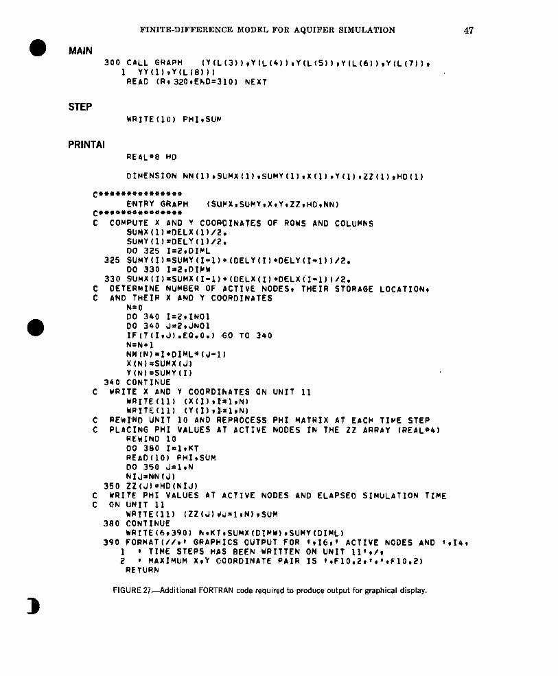
FINITE-DIFFERENCE MODEL FOR AQUIFER SIMULATION 47
MAIN 300 CALL GRAPH (Y(L(3))rYfL(Q)),Y(L(S))~Y(L(6))*Y(L(I))~
1 YY(l)vY(L(G))) READ (R, 320,EhD=310) NEXT
STEP WRITEtlO) PHIISUM
PRINTAI REAL”8 HD
C**4**#****u***0
ENTRY GRAPH (SUCX,SUMY,XvYtZZ,HO,NN) C****e********** C COMPUTE X AND Y COORCINATES OF ROWS AND COLUMNS
SUHX(l)=DELX(1~/2, SUMY(l)=DELY(l)/Z. DO 325 I=Z,DIML
325 SUMY~I~~SUMY~I~l~*~0ELY~I~~DELY~II1))/2. 00 330 1=2*DIMW
330 SUHX(I)=SUMX(I-~)*(DELX(I)*DELX~~-~))~~. C DETERMINE NUMBER OF ACTIVE NODES, THEIR STORAGE LOCATION, C AN0 THEIR X AND Y COORDINATES
N=O DO 340 I-2rINO1 DO 340 J=2rJNOl IF(T(IIJ).EO.O.) ,GO TO 340 N=N+l NN(N)=I*DIML*(J-1) X(N)=SlJHX(J) YtN)=SUHY(I)
340 CONTINUE C WRITE X AND Y COORDI,NATES ON UNIT 11
WRITE(11) tX(I)vE=l,N) WAITEtll) (Y(I) ,I:=l,N)
C REwrNO UNIT 10 AND REPROCESS PHI MATRIX AT EACH TIME STEP C PLACING PHI VALUES AT ACTIVE NODES IN THE ZZ ARRAY (REAL*41
REWIND 10 DO 380 I=lrKT READ(10) PHIsSUM DO 350 J=lrN NIJ=NN(J)
350 ZZ(J)=HD(NIJ) c WRITE PHI VALUES AT ACTIVE NODES AND ELAPSED SIMULATION TIME C ON UNIT 11
WRITEfll) (ZZ(J)dJ”lrN) *SUM 380 CONTINUE
wRItE(6r390) ktKT,SUMX(DIMW),SUMY(DIML) 390 FORMAT(//r@ GRAPHICS OUTPUT FOR (916,’ ACTIVE NODES AND *tIQr
1 ) TIME STEPS HAS BEEN WRITTEN ON UNIT ll’v/v 2 ) MAXIMUM XvY COORDINATE PAIR IS @~F10.2~‘,‘,F10.2)
RETURN
FIGURE 27,Additional FORTRAN code required to produce output for graphical display.
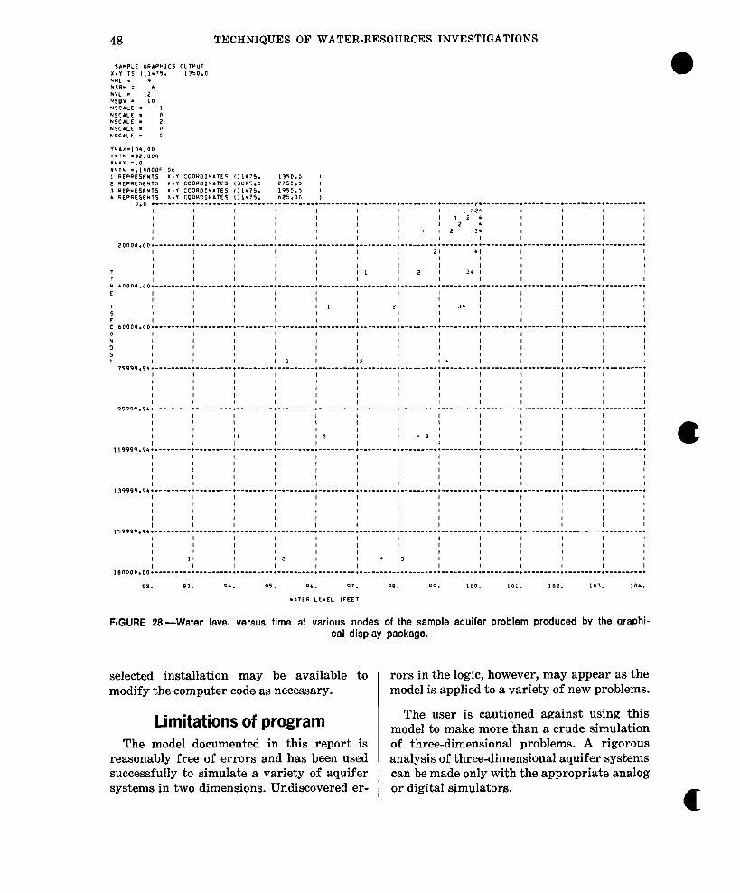
48 TECHNIQUES OF WATER-RESOURCES INVESTIGATIONS
I 1 I I 1 2 I i 6 13 I I I I I I I I I I I I I I I I 1 I I
18000~.00.---------*---------.---------.---------. -------_-.__----__-.---------.---------*---------.---------.---------.---------.
92. 93. 94. 95. 96. PI. 98. PP. 100. 101. LO.?. 103. 10..
WATER LEVEL IFEET,
FIGURE 28.-Water level versus time at various nodes of the sample aquifer problem produced by the graphi- cal display package.
selected installation may be available to rors in the logic, however, may appear as the modify the computer code as necessary. model is applied to a variety of new problems.
Limitations of program The user is cautioned against using this model to make more’than a crude simulation
The model documented in this report is of three-dimensional problems. A rigorous reasonably free of errors and has been used analysis of three-dimensional aquifer systems successfully to simulate a variety of aquifer can be made only with the appropriate analog systems in two dimensions. Undiscovered er- or digital simulators.
c
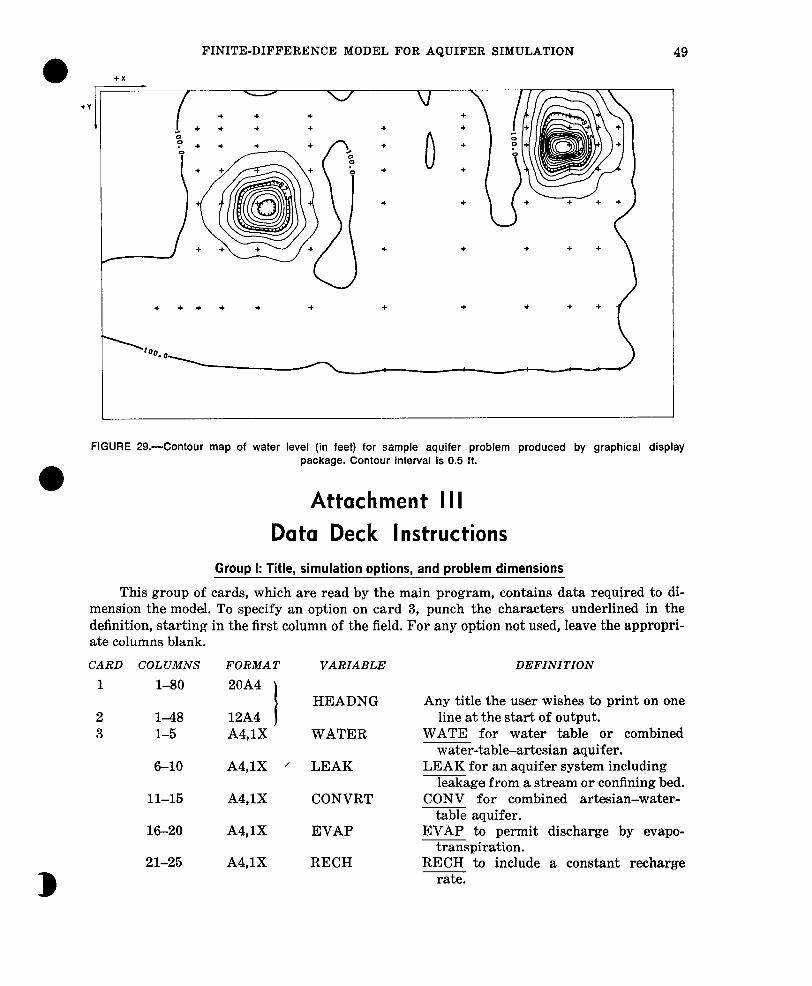
FINITE-DIFFERENCE MODEL FOR AQUIFER SIMULATION 49
FIGURE 29.-Contour map of water level (in feet) for sample aquifer problem produced by graphical display package. Contour interval is 0.5 ft.
Attachment I I I
Data Deck Instructions
Group I: Title, simulation options, and problem dimensions
This group of cards, which are read by the main program, contains data required to di- mension the model. To specify an option on card 3, punch the characters underlined in the definit,ion, starting in the first column of the field. For any option not used, leave the appropri- ate columns blank.
CARD COLUMNS
1 l-80
2 143 12A4 3 1-5 A4,lX
6-10
11-15
16-20
21-25
FORMAT
20A4
A4,lX ’
A4,lX
A4,lX
A4,lX
VARIABLE DEFINITION
HEADNG
WATER
LEAK
CONVRT
EVAP
RECH
Any title the user wishes to print on one line at the start of output.
WATE for water table or combined water-table-artesian aquifer.
LEAK for an aquifer system including leakage from a stream or confining bed.
CONV for combined artesian-water- table aquifer.
EVAP to permit discharge by evapo- transpiration.
RECH to include a constant rechargre rate.
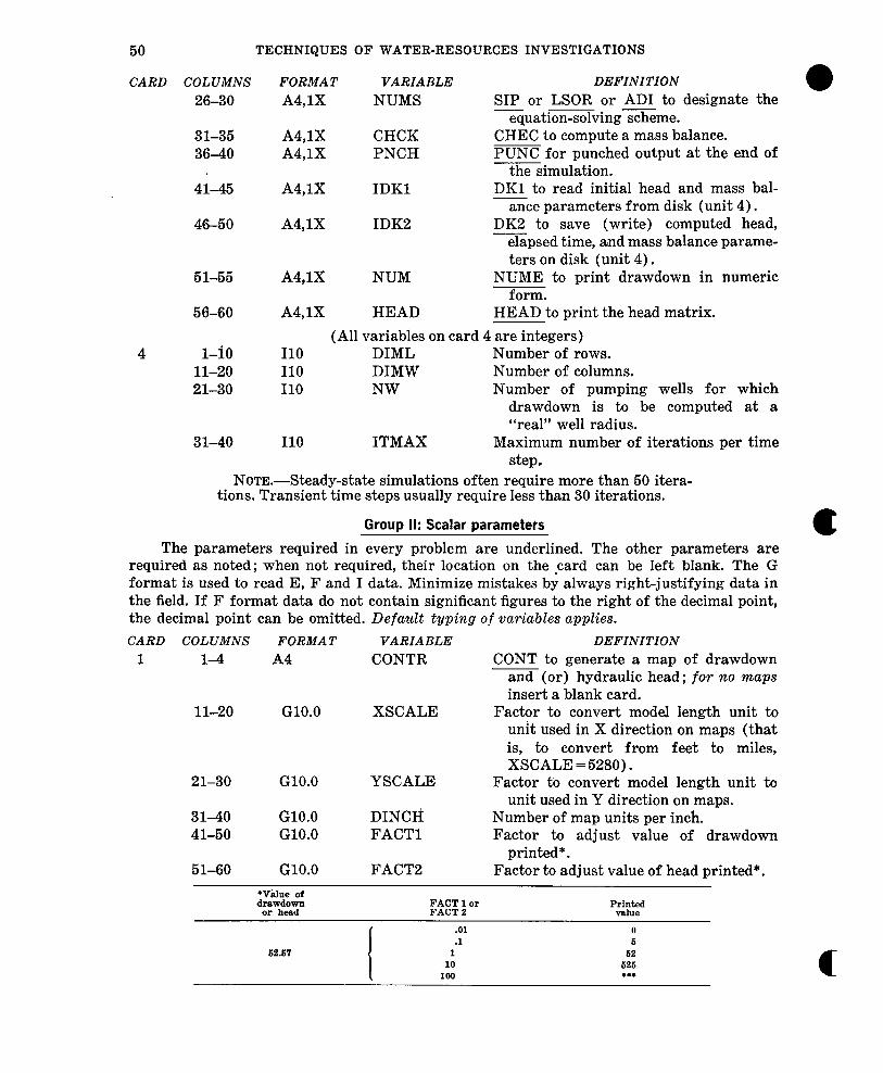
50 TECHNIQUES OF WATER-RESOURCES INVESTIGATIONS
CARD COLUMNS 2630
31-35 36-40
41-45
46-60
51-55
56-60
4 i-i0 11-20 21-30
31-40
FORMAT VARIABLE DEFINITION
A4,lX NUMS SIP or LSOR or AD1 to designate the equation-solving scheme.
A4,lX CHCK CHEC to compute a mass balance. A4,lX PNCH PUNC for punched output at the end of
the simulation. A4,lX IDKl DKl to read initial head and mass bal-
ance parameters from disk (unit 4). A4,lX IDK2 DK2 to save (write) computed head,
elapsed time, and mass balance parame- ters on disk (unit 4).
A4,lX NUM NUME to print drawdown in numeric form.
A4,lX HEAD HEAD to print the head matrix. (All variables on card 4 are integers)
110 DIML Number of rows. 110 DIMW Number of columns. 110 NW Number of pumping wells for which
drawdown is to be computed at a “real” well radius.
110 ITMAX Maximum number of iterations per time step.
NOTE.-Steady-state simulations often require more than 50 itera- tions. Transient time steps usually require less than 30 iterations.
Group II: Scalar parameters
The parameters required in every problem are underlined. The other parameters are required as noted ; when not required, their location on the *card can be left blank. The G format is used to read E, F and I data. Minimize mistakes by always right-justifying data in the field. If F format data do not contain significant figures to the right of the decimal point, the decimal point can be omitted. Default typing of variables applies. CARD COLUMNS FORMAT VARIABLE DEFINITION
1 l-4 A4 CONTR CONT to generate a map of drawdown and (or) hydraulic head ; for no maps insert a blank card.
11-20 G1O.O XSCALE Factor to convert model length unit to unit used in X direction on maps (that is, to convert from feet to miles, XSCALE = 5280).
21-30 G1O.O Y SCALE Factor to convert model length unit to unit used in Y direction on maps.
31-40 G1O.O DINCH Number of map units per inch. 41-50 G1O.O FACT1 Factor to adjust value of drawdown
printed*. 51-60 G1O.O FACT2 Factor to adjust value of head printed*.
+Vihle of drawdown
or head
69.67
FACT 1 or Printed FACT 2 value
.Ol 0
.l 6 1 62
10 626 100 l . . c
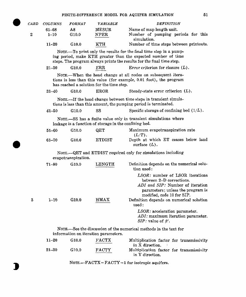
FINITE-DIFFERENCE MODEL FOR AQUIFER SIMULATION 51
CARD COLUMNS FORMAT VARIABLE DEFINITION
61-63 A8 MESUR Name of map length unit. 2 l-10 GlO.O NPER Number of pumping periods for this
simulation. 11-20 G1O.O KTH Number of time steps between printouts.
NOTE.-TO print only the results for the final time step in a pump- ing period, make KTH greater than the expected number of time steps. The program always prints the results for the final time step.
2130 GlO.O ERR Error criterion for closure (L) .
NOTE.-When the head change at all nodes on subsequent itera- tions is less than this value (for example, 0.01 foot), the program has reached a solution for the time step.
31-40 GlO.O EROR Steady-state error criterion (L) .
NOTE.-If the head change between time steps in transient simula- tions is less than this amount, the pumping period is terminated.
41-50 GlO.O ss Specific storage of confining bed (l/L).
NOTE.-SS has a finite value only ip transient simulations where leakage is a function of storage in the confining bed.
51-60 GlO.O &ET Maximum evapotranspiration rate (L/T).
61-70 GlO.O ETDIST Depth at which ET ceases below land surface (L) .
NOTE.--&ET and ETDIST required only for simulations including evapotranspiration.
71-30 GlO.O LENGTH Definition depends on the numerical solu- tion used:
3 l-10 G1O.O HMAX
LSOR: number of LSOR iterations between 2-D corrections.
ADZ and SIP: Number of iteration parameters ; unless the program is modified, code 10 for SIP.
Definition depends on numerical solution used :
LSOR : acceleration parameter. ADZ: maximum iteration parameter. SIP: value of p’.
NOTE.-See the discussion of the numerical methods in the text for information on iteration parameters.
11-20 G1O.O FACTX Multiplication factor for transmissivity in X direction. i
21-30 GlO.O FACTY Multiplication factor for transmissivity in Y direction.
NOTE .-FACTX = FACTY = 1 for isotropic aquifers.
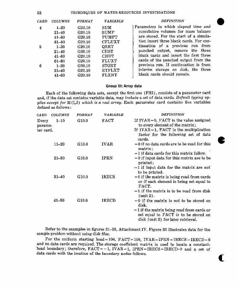
52 TECHNIQUES OF WATER-RESOURCES INVESTIGATIONS
CARD COLUMNS
4 l-20 21-40 41-60 61-80
5 l-20 21-40 41-60 61-80
6 l-20 21-40 41-60
FORMAT
G20.10 G20.10 G20.10 G20.10 G20.10 G20.10 G20.10 G20.10 G20.10 G20.10 G20.10
VARIABLE
SUM
SUMP PUMPT CFLUXT QRET CHST CHDT FLUXT STORT ETFLXT FLXNT
DEFINITION
Parameters in which elapsed time and cumulative volumes for mass balance are stored. For the start of a simula- tion insert three blank cards. For con- tinuation of a previous run from
. punched output, remove the three blank cards and insert the first three cards of the punched output from the previous run. If continuation is from interim storage on disk, the three blank cards should remain.
Group III: Array data
Each of the following data sets, except the first one (PHI), consists of a parameter card and, if the data set contains variable data, may include a set of data cards. Default typing ap- plies excetit for M (1,J) which is a real array. Each parameter card contains five variables defined as follows :
CARD COLUMNS
Every l-10 parame- ter card.
FORMAT VARIABLE
G1O.O FACT
11-20 G1O.O IVAR
21-30 G1O.O IPRN
31-40
41-50
G1O.O IRECS
G1O.O IRECD
DEFINITION
If IVAR=O, FACT is the value assigned to every element of the matrix ;
If IVAR= 1, FACT is the multiplication factor for the following set of data cards.
= 0 if no data cards are to be read for this matrix ;
’ = 1 if data cards for this matrix follow. =0 if input data for this matrix are to be
printed ; -1 if input data for the matrix are not
to be printed. = 0 if the matrix is being read from cards
or if each element is being set equal to FACT.
= 1 if the matrix is to be read from disk (unit 2).
=0 if the matrix is not to be stored on disk.
= 1 if the matrix being read from cards or set equal to FACT is to be stored on disk (unit 2) for later retrieval.
Refer to the examples in figures 31-33, Attachment IV. Figure 33 illustrates data for the sample problem without using disk files.
For the uniform starting head = 100, FACT = 100, WAR = IPRN = IRECS = IRECD = 0 and no data cards are required. The storage coefficient matrix is used to locate a constant- head boundary; therefore, FACT= - 1, IVAR= 1, IPRN= IRECS= IRECD=O and a set of data cards with the location of the boundary nodes follows.
c
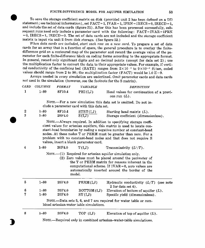
FINITE-DIFFERENCE MODEL FOR AQUIFER SIMULATION 53
To save the storage coefficient matrix on disk (provided un,it 2 has been defined on a DD statement; see technical information), set FACT = 1, IVAR = 1, IPRN = IRECS = 0, IRECD = 1, and include the set of data cards (figure 31). After this has been processed successfully, sub- sequent runs need only include a parameter card with the following : FACT = IVAR = IPRN = 0, IRECS= 1, IRECD=O. The set of data cards are not included and the storage coefficient matrix is input via unit 2 from disk storage. (See figure 32.)
When data cards are included, start each row on a new card. To prepare a set of data cards for an array that is a function of space, the general procedure is to overlay the finite- difference grid on a contoured map of the parameter and record the average value of the pat rameter for each finitedifference block on coding forms according to the appropriate format. In general, record only significant digits and no decimal points (except for data set 2) ; use the multiplication factor to convert the data to their appropriate values. For example, if verti- cal conductivity of the confining bed (RATE) ranges from 2X lo+ to 9 x 1O-s ft/sec, coded values should range from 2 to 90; the multiplication factor (FACT) would be 1.0 E -9.
Arrays needed in every simulation are underlined. Omit parameter cards and data cards not used in the simulation (however, see the footnote for the S matrix).
CARD COLUMNS FORMAT VARIABLE DEFINITION
1 l-80 8F10.4 PHI (1,J) Head values for continuation of a previ- ous run (L).
NOTE.-For a new simulation this data set is omitted. Do not in- clude a parameter card with this data set.
2 l-80 8F10.4 STRT(I,J) St,arting head matrix (L) . 3 l-80 20F4.0 SC&J) Storage coefficient (dimensionless).
NOTE.-Always required. In add:ition to specifying storage coeffi- cient values for artesiain aquifers, this matrix is used to locate con- stant-head boundaries by coding a negative number at constant-head nodes. At these nodes T or PERM must be greater than zero. For a problem with no constant-head nodes and that does not require S values, insert a blank parameter card.
4 l-80 20F4.0 T t&J) Transmissivity (U/T).
NOTE.- (1) Required for artesian aquifer simulation only. (2) Zero values must be placed around the perimeter of
the T or PERM matrix for reasons inherent in the computational scheme. If IVAR=O, zero values are automatically inserted around the border of the model.
5 l-80 20F4.0 PERM (1,J) Hydraulic conductivity (L/T) (see note 2 for data set 4).
6 l-80 20F4.0 BOTTOM (1,J) Elevation of bottom of aquifer (L) . 7 l-80 20F4.0 SY U,J) Specific yield (dimensionless) .
NOTE.-Data sets 5, 6, and 7 are required for water table or com- bined artesian-water table simulations.
8 l-80 20F4.0 TOP (1,J) Elevation of top of aquifer (L) .
NOTE.-Required only in combined artesian-water-table simulations.
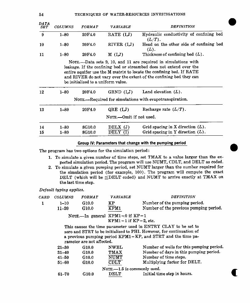
54 TECHNIQUES OF WATER-RESOURCES INVESTIGATIONS
DATA SET COLUMNS FORMAT VARIABLE DEFINITION
9 l-80 20F4.0 RATE (1,J) Hydraulic conductivity of confining bed (L/T).
10 l-80 20F4.0 RIVER (1,J) Head on the other side of confining bed W) *
11 l-80 20F4.0 M (LJ) Thickness of confining bed (L) .
NOTE.-Data sets 9, 10, and 11 are required in simulations with leakage. If the confining bed or streambed does not extend over the entire aquifer use the M matrix to locate the confining bed. If RATE and RIVER do not vary over the extent of the confining bed they can be initialized to a uniform value.
12 1~80 20F4.0 GRND (1,J) Land elevation (L) .
NOTE.-Required for simulations with evapotranspiration.
13 l-80 20F4.0 QRE (LJ) Recharge rate (L/T).
NOTE.-omit if not used.
14 l-80 8GlO.O DELX (J) Grid spacing in X direction (L) . 15 l-80 8GlO.O DELY (I) Grid spacing in Y direction (L) .
Group IV: Parameters that change with the pumping period
The program has two options for the simulation period : 1. To simulate a given number of time steps, set TMAX to a value larger than the ex-
pected simulation period. The program will use NUMT, CDLT, and DELT as coded. 2. To simulate a given pumping period, set NUMT larger than the number required for
the simulation period (for example, 100). The program will compute the exact DELT (which will be SDELT coded) and NUMT to arrive exactly at TMAX on the last time step.
Default typing applies.
CARD COLUMNS FORMAT VARIABLE DEFINITION
1 l-10 G1O.O KP Number of the pumping period. 1 l-20 G1O.O KPMl Number of the previous pumping period.
Nom.-In general KPMl =.O if KP= 1 KPMl = 1 if KP = 2, etc.
This causes the time parameter used in ENTRY CLAY to be set to zero and STRT to be initialized to PHI. However, for continuation of a previous pumping period KPMl=KP, and STRT and the time pa- rameter are not affected.
21-30 G1O.O NWEL Number of wells for this pumping period. 31-40 G1O.O TMAX Number of days in this pumping period. 41-50 G1O.O NUMT Number of time steps. 51-60 G1O.O CDLT Multiplying factor for DELT.
NOTE .-1.5 is commonly used. 61-70 G1O.O DELT Initial time step in hours. c
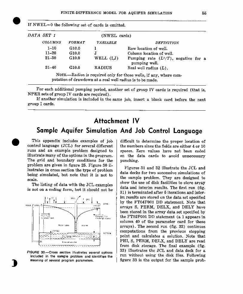
FINITE-DIFFERENCE MODEL FOR AQUIFER SIMULATION 55
If NWEL=O the following set of cards is omitted.
DATA SET 1 (NWEL cards)
COLUMNS FORMAT VARIABLE DEFINITION l-10 G1O.O 1 Row location of well.
11-20 G1O.O J Column location of well. 2130 G1O.O WELL (1,J) Pumping rate (U/T), negative for a
pumping well. 31-40 G1O.O RADIUS Real well radius (L) .
NOTE.-Radius is required only for those wells, if any, where com- putation of drawdown at a real well radius is to be made.
For each additional pumping period, another set of group IV cards is required (that is, NPER sets of group IV cards are required).
If another simulation is included in the same job, insert a blank card before the next group I cards.
Attachment IV
Sample Aquifer S,imulation And Job Control Language
0 This appendix includes examples of job control language (JCL) for several different runs and an example problem designed to illustrate many of the options in the program. The grid and boundary conditions for the problem are given in figure 25. Figure 30 il- lustrates in cross section the type of problem being simulated, but note that it is not to scale.
The listing of data with the JCL examples is not on a coding form, but it should not be
FIGURE 30.-Cross section illustrates several options included in the sample problem and identifIesI the
3
meaning of several program parameters.
difficult to determine the proper location of the numbers since the fields are either 4 or 10 spaces. Zero values have not been coded on the data cards to avoid unnecessary punching.
Figures 31 and 32 illustrate the JCL and data decks for two successive simulations of the sample problem. They are designed to show the use of disk facilities to store array data and interim results. The first run (fig. 31) is terminated after 5 iterations and inter- im results are stored on the data set specified by the FT04FOOl DD statement. Note that arrays S, PERM, DELX, and DELY have been stored in the array data set specified by the FT02FOOl DD statement (a 1 appears in column 40 of the parameter card for these arrays). The second run (fig. 32) continues computations from the previous stopping point and calculates a solution. Note that PHI, S, PERM, DELX, and DELY are read from disk storage. The final example (fig. 33) illustrates the JCL and data deck for a run without using the disk files. Following figure 33 is the output for the sample prob-
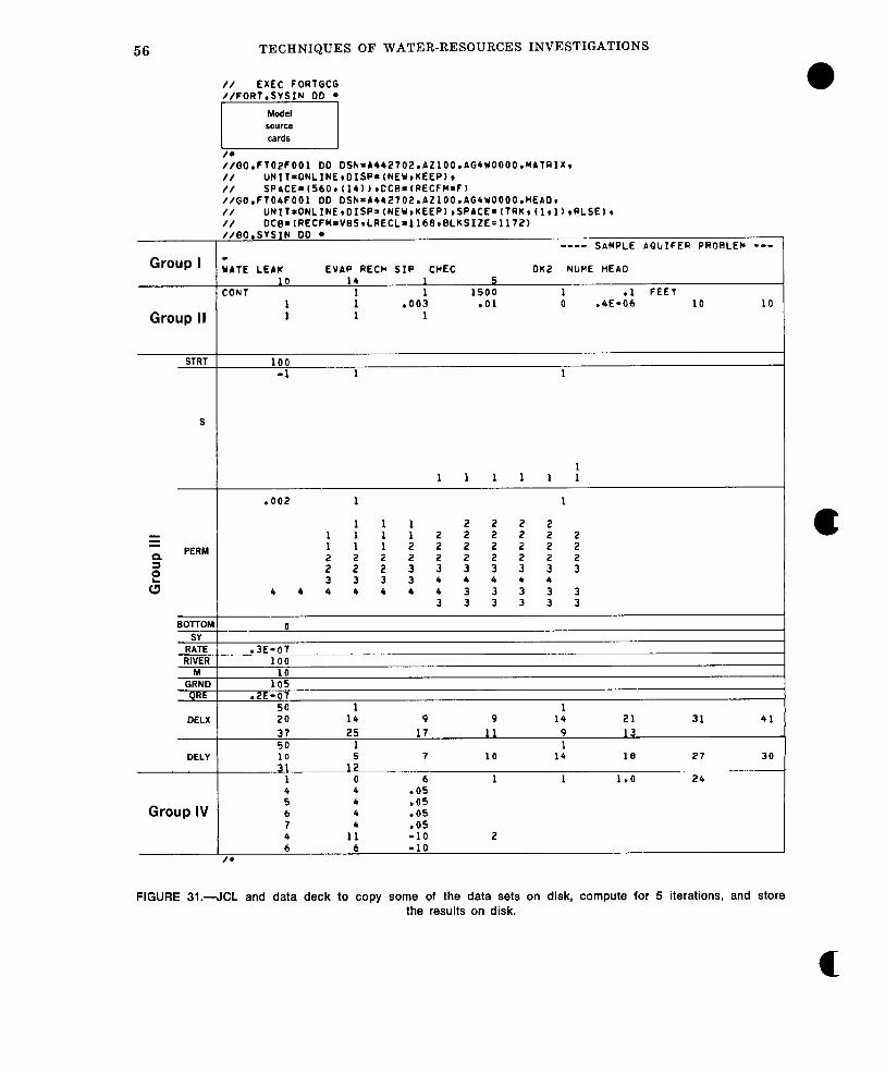
56 TECHNIQUES OF WATER-RESOURCES INVESTIGATIONS
EXEC FORTGCG //FORT.SYSIN DO l
/* //GO.F102FOOl DO DSk=A442702.Ai!100.AG4UOOOO.MATRIX( // UNIT=ONLINEtDISP=~NEU~KEEP)r // SPACE=~~~O.~~~~~~OC~=~RECFM=F~ //GO.F104FOOl DO OSN=A442702.AZ100.AG4WOOOO.HEAO~ // UNIt+ONLINEtOISP~~NEU~KEEPl~SPACE=~lRK~~l~l~~RLSE~~ // OCB=~RECFM=VBS~LRECL=~~~EI~BLKSIZE=~~T~~ //QO.SYSIN 00 l
---- SAMPLE AQUIFER PROBLEM ---
Group ’ EATE LEAK EVAP RECH SIP CHEC DK2 NUME HEAD 10 14 1 5
CON1 1 1500 1 .l FEET 1 .003 .Ol 0 .4E-06 10 10
Group II 1 1 1
STRT 100 -1 1 1
s
1 1 1 1 1 :
.002 1 1
1 1 1 2 2 2 2 1 1 ; 2 2 2 2 2 1 1 2 2 2 2 2
f 3 3 3 3 4 4 4 4 4
4 4 4 4 4 4 4 3 3 3 3 3 3 3 3 3 3 3
BOTTOM 0 SY
RATE .3E-07 RIVER 100
M GRND QRE .2E-07
50 1 1 DELX 20 14 9 9 14 21 31 41
37 25 17 11 9 13 50 1 1
DELY 10 5 7 10 14 18 27 30 31 12
1 0 6 1 1 1.0 24 4 .05 4
Group IV .05
6 4 .05 ?
1: .05
4 -10 2 6 6 -10
/*
FIGURE 31.-JCL and data deck to copy some of the data sets on disk, compute for 5 iterations, and store the results on disk.
c
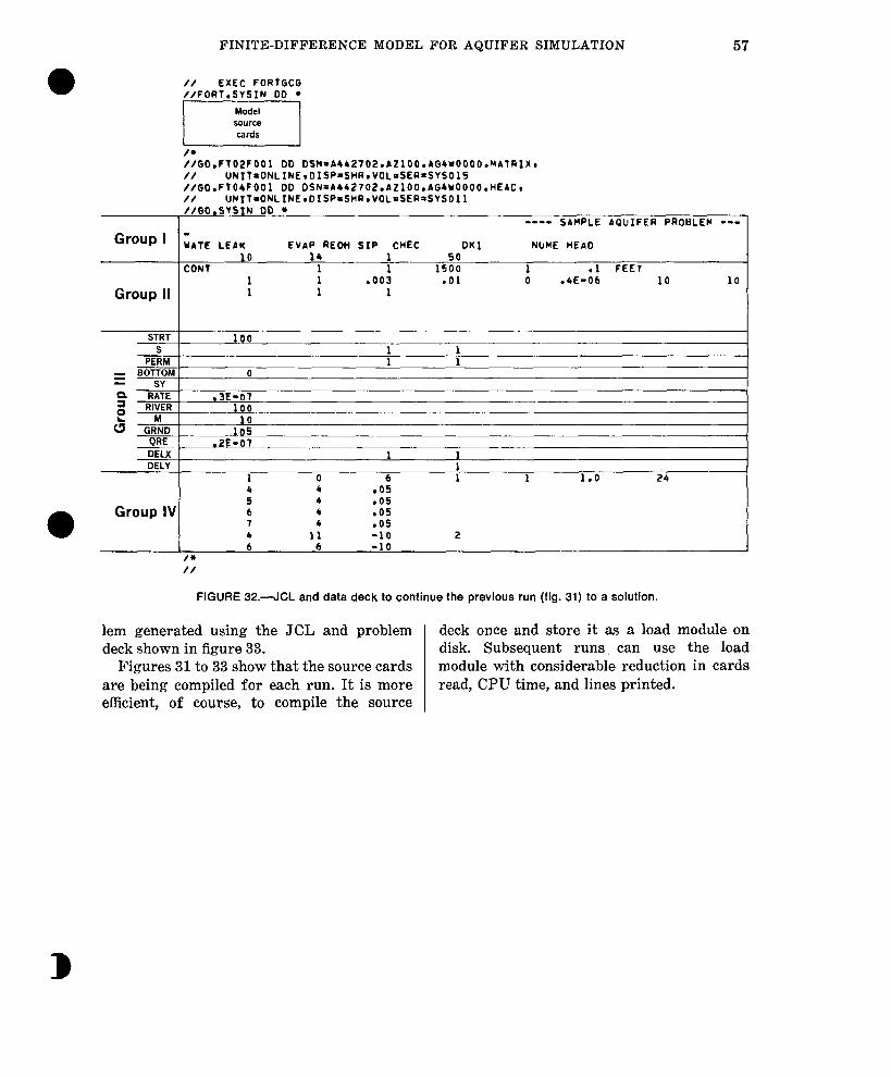
FINITE-DIFFERENCE MODEL FOR AQUIFER SIMULATION 57
EXEC FORTGCG //FORT.SYSIN 00 l
f----l
Model source cards
/* //GO.F102F001 DO OSk=A442702.A2l00.AG4WOOOO.~AlRIX~ // lJN~T=ONLINE~OISP=SHR~VOL=SER=SYSOl5 //GO.FTO4FOOl 00 OSN=A442702.A2l00.AG4UOOOO.HEAO~ // UNIt=ONLINErOISP=SHR~VOL=SER=SYSOll //GO,SYSIN 00 l
---- SAMPLE AQUIFER PROBLEM ---
Group ’ tATE LEAK EVAP REOH SIP CHEC OK1 NllME HEAO 10 I4 1 50
CONT 1 1500 1 .l FEET
Group II :
: ,003 .Ol 0 .4E-06 10 10
1 1
STRT 100 s I 1
PEiM i i I BOTTOM 0
SY RATE ,3E-07 -- RIVER .--!d!L---~- -~-
M 1 GRNO 10; QRE .2E-07 --. IXLX 1 1 DELY
1 0 6 t 1 1.0 24 4 4 .05 5 4 .05
Group IV 6 4 .05 7 4 .05 4 11 -10 2 6 6 -10
/* //
FIGURE 32.-JCL and data deck to continue the previous run (fig. 31) to a solution.
lem generated using the JCL and problem deck once and store it as a load module on deck shown in figure 33. disk. Subsequent runs, can use the load
Figures 31 to 33 show that the source cards module with considerable reduction in cards are being compiled for each run. It is more read, CPU time, and lines printed. efficient, of course, to compile the source
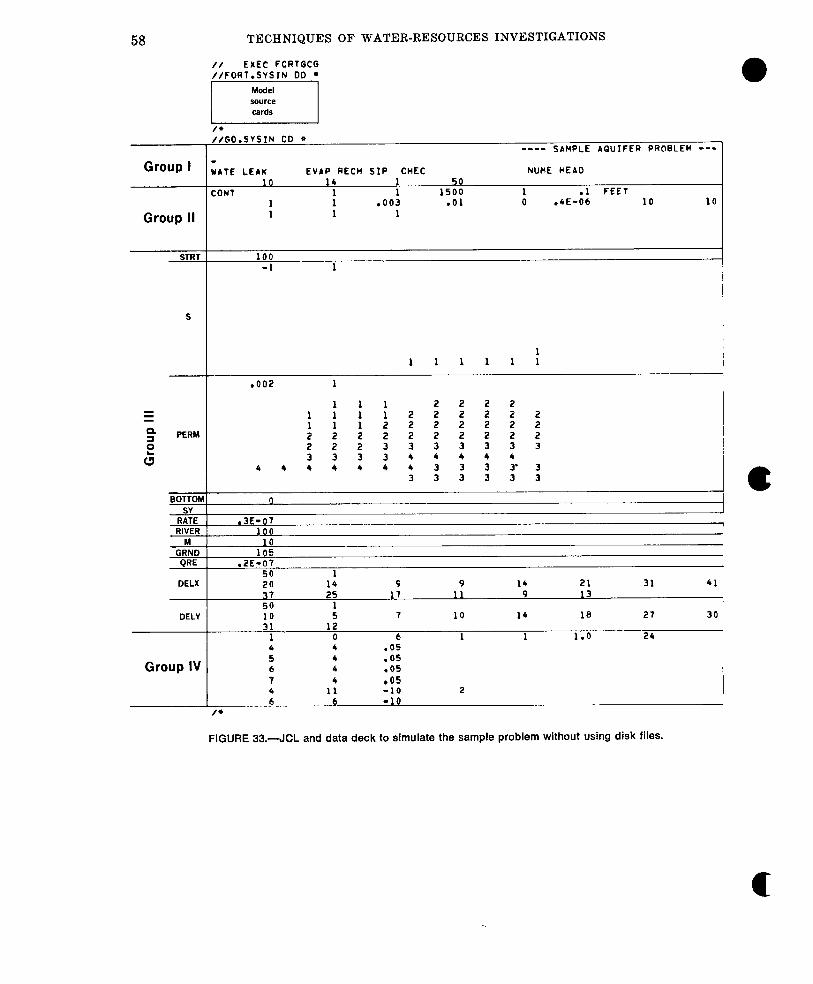
58
Group I
Group II
STRT
s
BOTTOL sy
RATE RIVER
M GRND
QRE
DELX
DELY
Group IV
TECHNIQUES OF WATER-RESOURCES INVESTIGATIONS
EXEC FORTGCG //FORT.SYSIN DO *
r/GO.SYSIN OD * ---- SAMPLE AQUIFER PROBLEM ---
lATE LEAK EVAP RECH SIP CHEC NUHE HEAD 10 14 1
ZONT : 1 1 .l FEET 1 ,003 .Ol 0 .4E-06 10 10 1 1 1
100 -1 1
1 1 1 1 1 1 1
,002 1
: 1
: 1 : 2 s
2 2 2
: 2 2 2 2 2 2
2 f 2 2 2 2 2 s 2 2 2 2 2 2 : 3 3 3 3 3 3 3 3 : 4 4 4 4 4
44444443333-3 3 3 3 3 3 3
.3 - 7
10 105
.2E-07
50 20 12 9 9 14 21 31 41 37 25 17 11 9 13 50 1 10 5 7 10 14 18 27 30 31 12
1 0 6 1 1 1.0 24
: 4 4 .05 .OS 6 4 .05 7 4 r05 4 11 -10 2
FIGURE 33.-JCL and data deck to simulate the sample problem without using disk files.
c
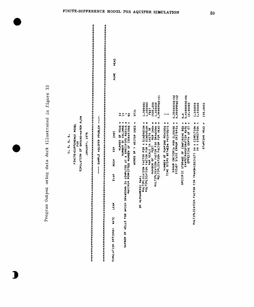
FINITE-DIFFERENCE MODEL FOR AQUIFER S!B&ULATION
: : : : : : : : t i : : t t : : : : : : : t : : :
8 l
i t *
: :
: d l
E I’
:
t :
:: 0
0’ :
Q t
w :
1 t
: : 0
: :
: :
: l
:
:
:
t
t
:
:
:
:
:
: .
:
:
: l
:
i
i
:
:
:
i
59
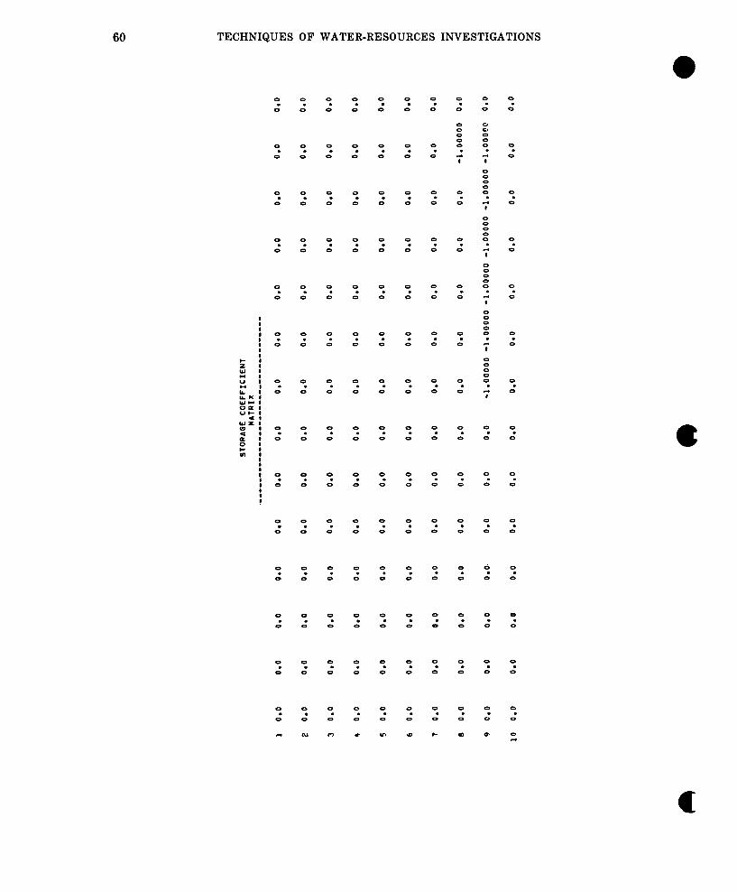
TECHNIQUES OF WATER-RESOURCES INVESTIGATIONS
0 d
0 .
0
0 .
0
0 .
Q
0 .
0
0 .
0
0 d
Q .
0
0 .
0
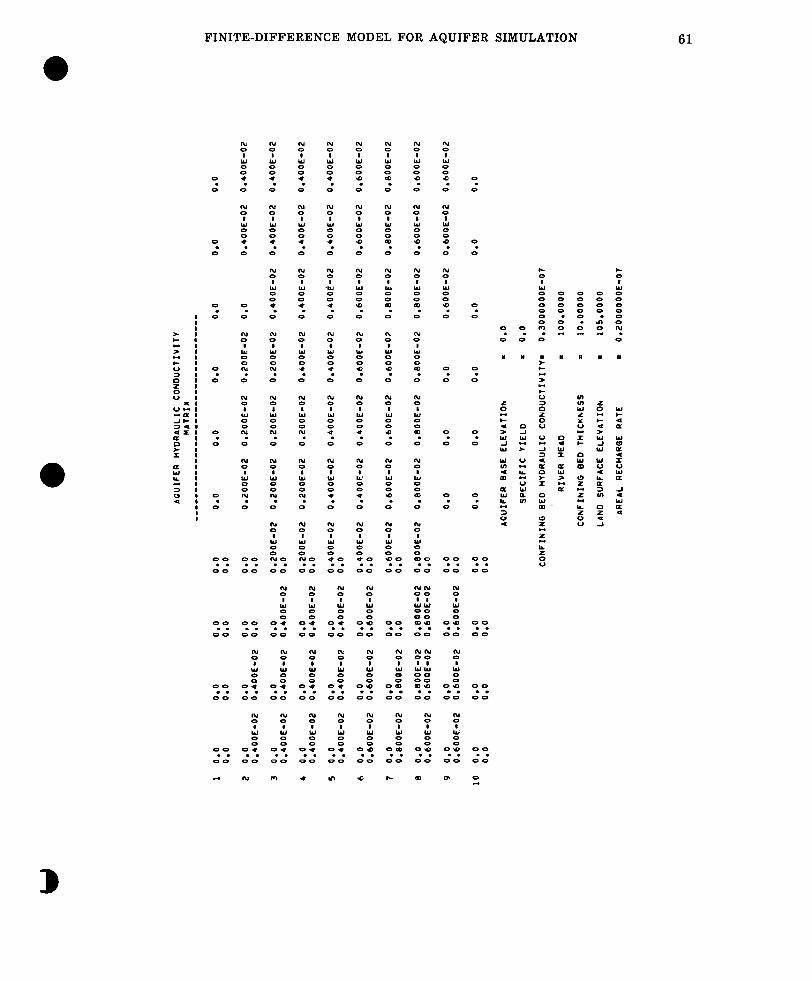
FINITE-DIFFERENCE MODEL FOR AQUIFER SIMULATION 61
,” :: . * f: 0
. 0
*
Q .
Q
n Y
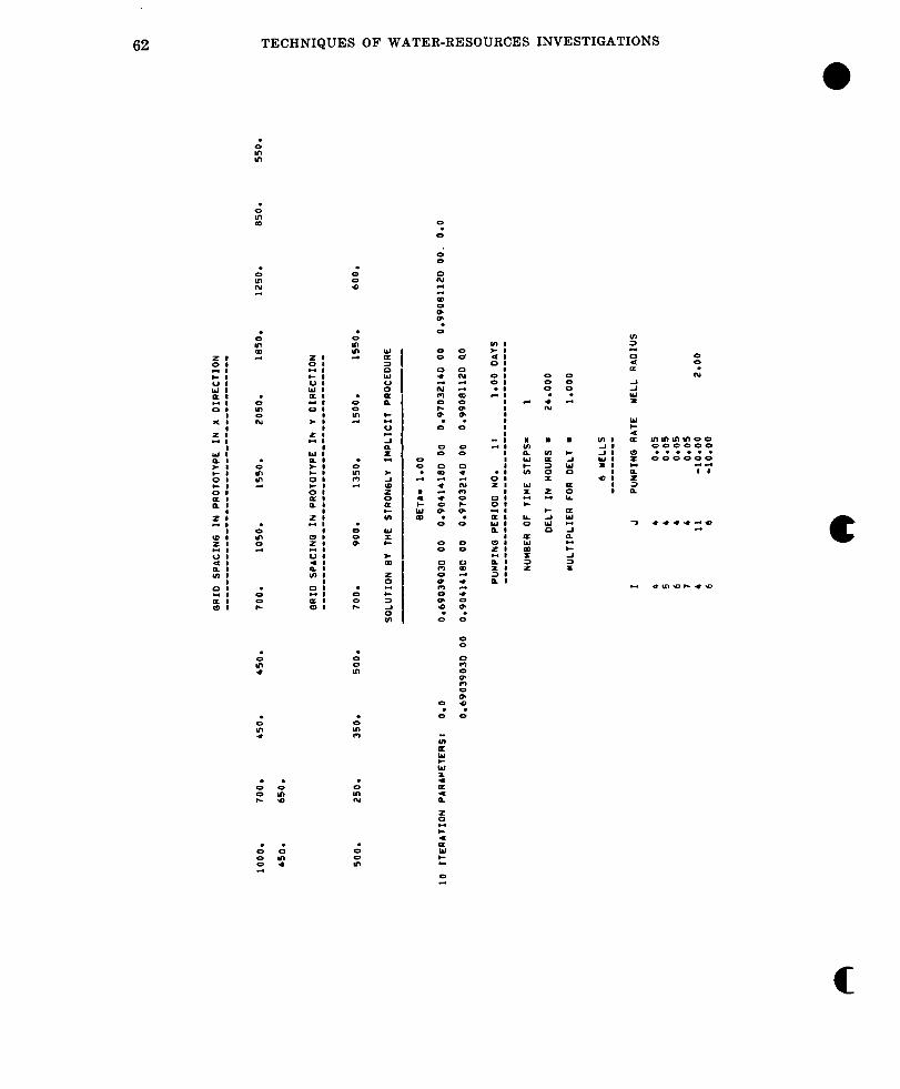
62 TECHNIQUES OF WATER-RESOURCES INVESTIGATIONS
z Q . f
z Q .
c
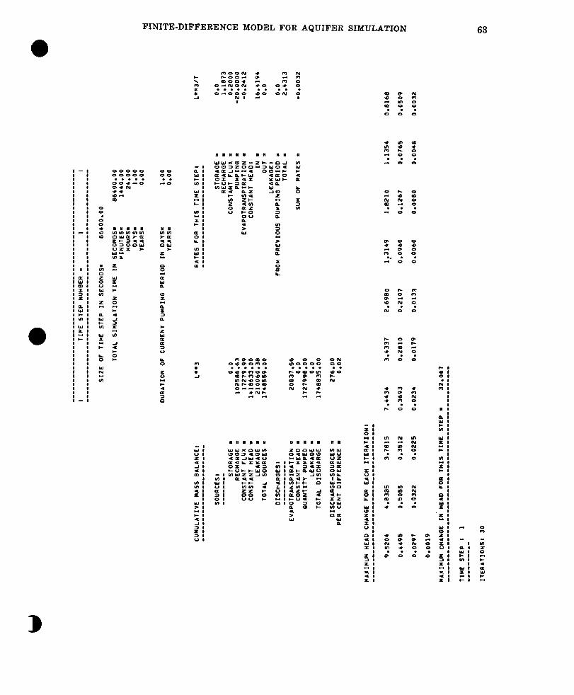
FINITE-DIFFERENCE MODEL FOR AQUIFER SIMULATION
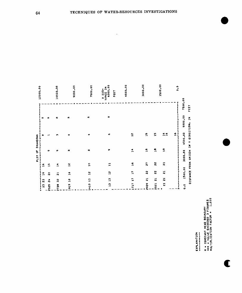
64 TECHNIQUES OF WATER-RESOURCES INVESTIGATIONS
----•--
l
o- ---*
LB If
---- .-- --
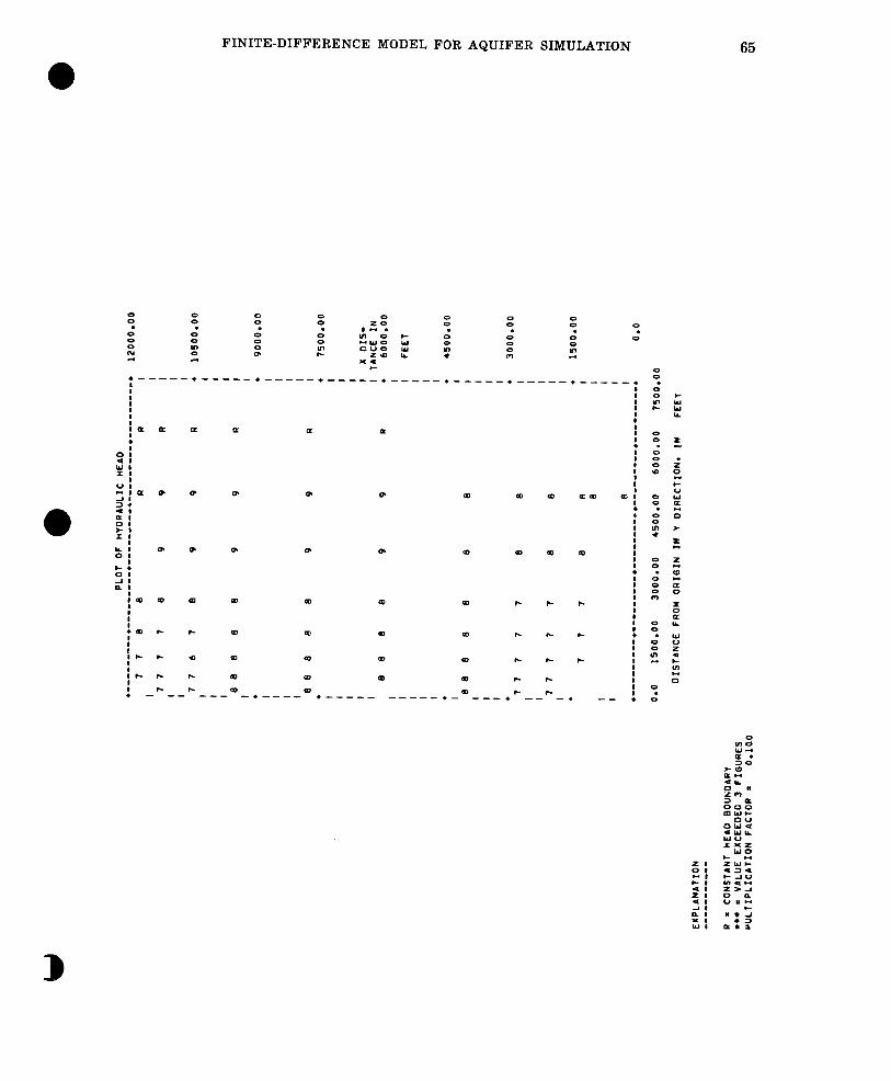
FINITE-DIFFERENCE MODEL FOR AQUIFER SIMULATION
I i IC c :
mm
a
c
r‘
r-
ir- r- I E
I c I 0
I- ro 0 + a0 r- - -- --- -*----w l ----- :
-----*- ---* --‘-. -- l 0’
65
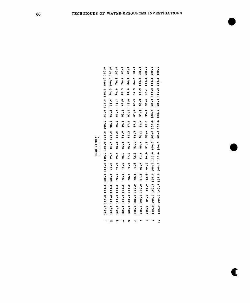
TECHNIQUES OF WATER-RESOURCES INVESTIGATIONS
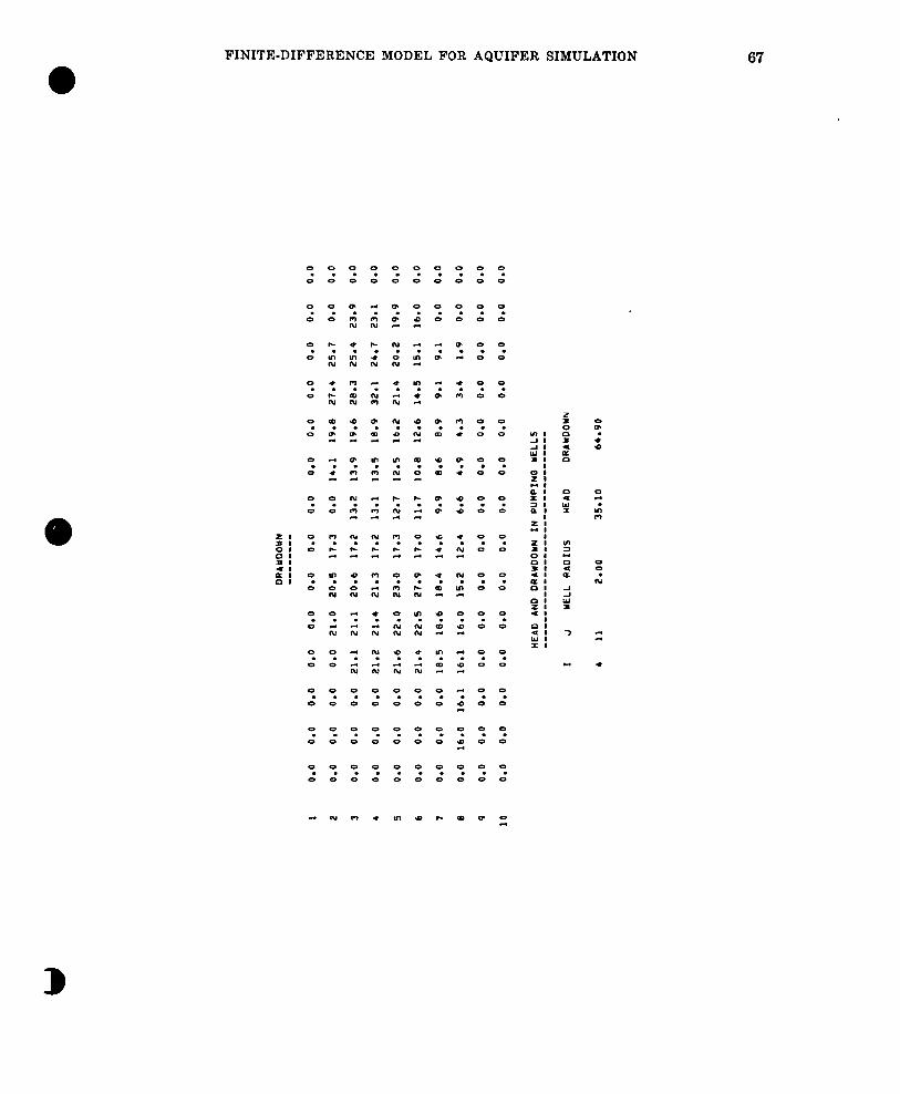
FINITE-DIFFERENCE MODEL FOR AQUIFER SIMULATION 67
0 .
0
(u . !I!
A .
f:
0 .
0
Q .
0
0 .
0
N . 2
N . I;
0 .
0
0 .
0
0 .
0
0 .
0
0 m . . z ;;
0 .
Q . z . N
l .
;;
0 .
Q
0 .
0
0 .
0
N .
N
0 .
0
0 .
0
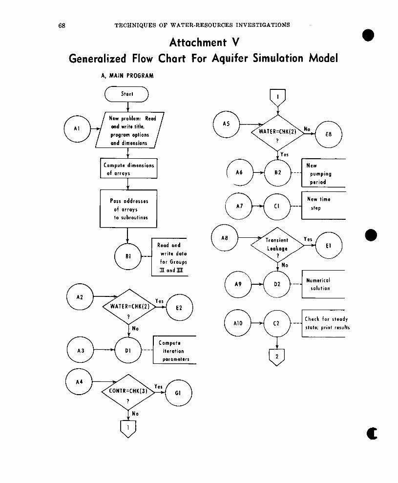
68 TECHNIQUES OF WATER-RESOURCES INVESTIGATIONS
Attachment V
Generalized Flow Chart For Aquifer Simulation Model A, MAIN PROGRAM
f Start 1 \ / 1
New problem: Read
ond write title,
program options
and dimensions
1
j C;;:;;;y:mensions]
Pass addresses
0
Check for steady
state; print results
b I c
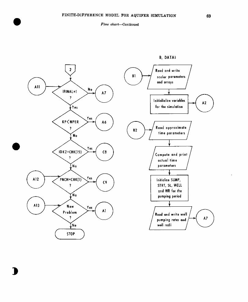
FINITE-DIFFERENCE MODEL FOR AQUIFER SIMULATION
Flow chart-Continued
B, DATAI
69
I +
I Compute and print
actual time parameters
+
Initialize SUMP,
STRT, 51, WELL
and WR far the
1 , pumpin; period ) ,
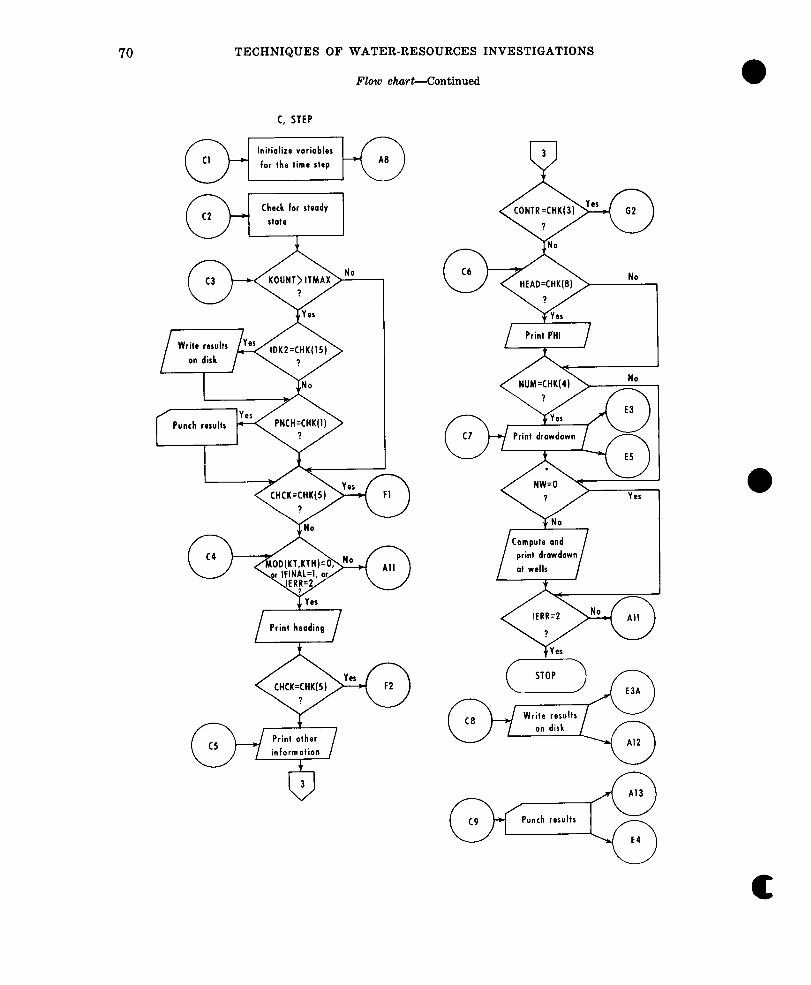
70 TECHNIQUES OF WATER-RESOURCES INVESTIGATIONS
Flow char&Continued
IDK2=CHKIISI
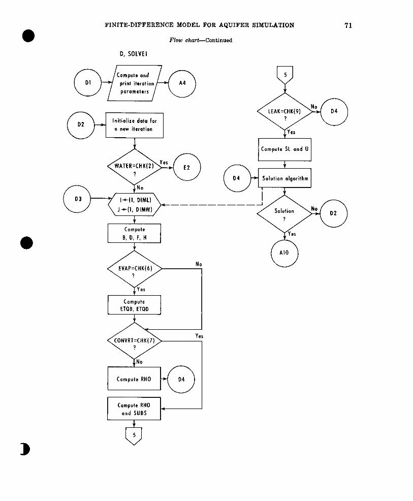
FINITE-DIFFERENCE MODEL FOR AQUIFER SIMULATION
Flow chart-Continued
D, SOLVEI
---- J+(l, DIMW)
71
( LEAK=CHK(9) w A Nn
3
D4
I Compute SL and U
0 Al0
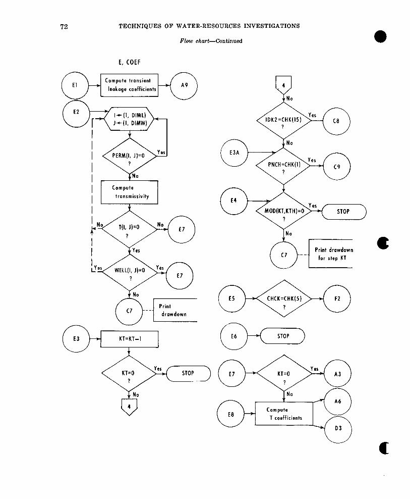
72 TECHNIQUES OF WATER-RESOURCES INVESTIGATIONS
Flow chart-Continued
E, COEF
@jEKLJ
I I Compute I i 1 trons;issivity 1
P ,4 No
INo
c
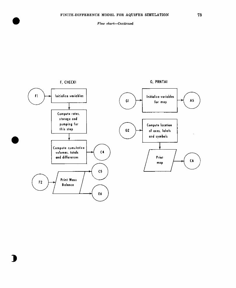
FINITE-DIFFERENCE MODEL FOR AQUIFER SIMULATION
Flow chartContinued
F, CHECKI
Compute cumulative volumes, totals
to
c4
and differences
G, PRNTAI
73
Compute location
of axes, labels
and symbols
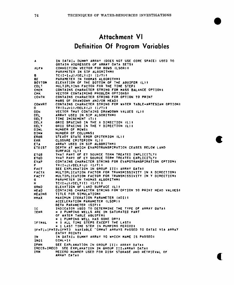
74 TECHNIQUES OF WATER-RESOURCES INVESTIGATIONS
A
ALFA
B GE BQTTOM CDL1 CHCK CHK CONTR
CONVRf 0 DON DEL DELT DELX DELY OIML DIMW EROR ERR ETA ETDIST
ETQG EfQD EVAP F FACT FACTX FACTY G H GRND HEAD HEADNG HMAX
XC IERR
IFINAL
Attachment VI
Definition Of Program Variables
IN DATA19 DUMMY ARRAY (DOES NOT USE CORE SPACE) USED TO OBTAIN ADDRESSES OF ARRAY DATA SETS: CORRECTION VECTOR FOR ROWS (LSOR): PARAMETER IN SIP ALGORITHM; TC(I-lrJ)/DELY(I) (l/T) i PARAMETER IN THOMAS ALGORITHM; ELEVATION OF THE BOTTOM OF THE AQUIFER (L)1 MULTIPLYING FACTOR FOR THE TIME STEP; CONTAINS CHARACTER STRING FOR MASS BALANCE OPTION! VECTOR CONTAINING PROBLEM OPTIONS; CONTAINS CHARACTER STRING FOR OPTION TO PRINT MARS OF DRAWDOWN AND/OR HEAD; CONTAINS CHARACTER STRING FOR WATER TABLE-ARTESIAN OPTION1 TR(IqJ-lI/DELX(J) (l/T): VECTOR THAT CONTAINS DRAWDOWN VALUES (L); ARRAY USED IN SIP ALGORITHM; TIHE INCREMENT (T)l GRID SPACING IN THE X DIRECTION (L) 8 GRID SPACING IN THE Y DIRECTION (L); NUMGER OF ROWS: NUMBER OF COLUMNS8 STEADY STATE EROR CRITERION (L)t CLOSURE CRITERION (L)I ARRAY USED IN SIP ALGORITHM: DEPTH AT WHICH EVAPOTRANSPIRATION CEASES BELOW LAND SURFACE (L) ; THAT PART OF El SOURCE TERM TREATED IMPLICITLY: THAT PART OF ET SOURCE TERM TREATED EXPLICITLY; CONTAINS CHARACTER STRING FOR EVAPOTRANSPIRATION OPTION1 TR(IrJ)/DELXtJ) (l/T) 8 SEE EXPLANATION IN GROUP IIIt ARRAY OATAl MULTIPLICATION FACTOR FOR TRANSMISSIVITY IN X DIRECTION8 MULTIPLICATION FACTOR FOR TRANSHISSIVITY IN Y DIRECTICN) PARAMETER IN THOMAS ALGORITHM8 TCtIwJ)/DELYfI) (l/T)1 ELEVATION OF LAND SURFACE (Lb; CONTAINS CHARACTER STRING FOR‘OPTION TO PRINT HEAD VALUES; TITLE FOR SIMULATION1 MAXIMUM ITERATION PARAMETER (AD111 ACCELERATION PARAMETER (LSOR); BETA PARAMETER (SIP) i INDICATOR USED TO DETERMINE THE TYPE OF ARRAY DATA8 = 0 PUNPING WELLS ARE IN SATURATED PART OF WATER TABLE AQUIFER: = 1 PUMPING WELL HAS GONE DRY: = 0 ALL TIME STEPS EXCEPT THE LAST; = 1 LAST TIME STEP IN PUMPING PERIOD; -
IFtdTlrIFMT2rIFMT3 VARIABLE -0RMAT ARRAYS PASSED TO DATA1 VIA ARRAY ENTRY POINT:
IN IN OATAII DUMMY ARRAY TO WHICH NAME IS PASSED: IN01 OIML-18 IPRN SEE EXPLANATION IN GROUP 1118 ARRAY DATA: ;;;CSeIRECD SEE EXPLANATION IN GROUP IIIgARRAY OATA;
RECORD NUMBER USED FOR DISK STORAGE AN0 RETRIEVAL OF ARRAY DATA: c
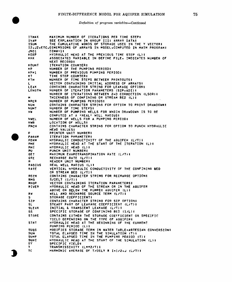
FINITE-DIFFERENCE MODEL FOR AQUIFER SIMULATION
Definition of program. variables--Continued
ITMAX MAXIMUM NUMGEA OF ITERATIONS PER TIME STEP8 IkAR SEE EXPLANATION IN GROUP III; ARRAY DATA: ISUM THE CUMULATIVE WORDS OF STORAGE USED IN THE Y VECTOR: IZrJZ~ElC.DIHENSIONS OF ARRAYS IN MODEL~COMPUTEO IN MAIN PROGRAM; JNOl DIMW-1 i KEEP KKK
HYDRAULIC HEAD AT THE PREVIOUS TIME STEP (Ll1 ASSOCIATED VARIABLE IN DEFINE FILE* INDICATES NUMBER OF NEXT RECORD1 ITERATION COUNTER; KOUNT
KP KPMl KT KTH L LEAK LENGTH
n NPER NUH NUMT NW
NWEL NWR PNCH
0 P PARAM PERM WE PHI PU QET QRE R RADIUS RATE
RECH RHO RHOP RIVER
RW S SIP SL SLEAK ss STORE
STRT
NUMBER OF THE PUMPING PERIOD: NUMBER OF PREVIOUS PUMPING PERIOD1 TIME STEP COUNTER8 NUMRER OF TIME STEPS BETWEEN PRINTOUTS; VECTOR CONTAINING INITIAL ADDRESS OF ARRAYS; CONTAINS CHARACTER STRING FOR LEAKAGE OPTION; NUMBER OF ITERATION PARAMETERS (SIPIADI); NUW@ER OF ITERATIONS BETWEEN 2-D CORRECTION (LSORlI THICKNESS OF CONFINING OR STREAM BED (L11 NUMBER OF PUMPING PERIODS; CONTAINS CHARACTER STRING FOR OPTION TO PRINT DRAWDOWNI NUMBER OF TIME STEPS: NUMBER OF PUMPING WELLS FOR WHICH DRAWDOWN IS TO BE COMPUTED AT A ‘REAL’ WELL RADIUSI NUMBER OF WELLS FOR A PUMPING PERIOOI LOCATION OF WELLS) CONTAINS CHARACTER STRING FOR OPTION TO PUNCH HYDRAULIC HEAD VALUES; PRINTER UNIT NUMBER: ITERATION PARAMETER8 HYDRAULIC CONDUCTIVITY OF THE AQUIFER (L/TlI HYDRAULIC HEAD AT THE START OF THE ITERATION (Lb8 HYDRAULIC HEAD (Lb; PUNCH UNIT NUMBER; MAXIMUM EVAPOTRANSPIRATION RATE (L/T); RECHARGE RATE (L/T) : READER UNIT NUMBER; REAL WELL RADIUS (LB: VERTICAL HYDRAULIC CONDUCTIVITY OF THE CONFINING BED OR STREAM BED (L/T): CONTAINS CHARACTER STRING FOR RECHARGE OPTION; S/DELT (l/T) I VECTOR CONTAINING ITERATION PARAMETERS; HYDRAULIC HEAD OF THE STREAM OR IN THE AQUIFER ABOVE OR BELOW THE PUMPED AQUIFER fL1: WELL AND RECHARGE SOURCE TERM (L/T1 1 STORAGE COEFFICIENT1 CONTAINS CHARACTER STRING FOR SIP OPTION; STEADY PART OF LEAKAGE COEFFICIENT (L/T); INITIAL 4 TRANSIENT LEAKAGE (L/T): SPECIFIC STORAGE OF CONFINING GED (l/L11 CONTAINS EITHER THE STORAGE COEFFICIENT OR SPECIFIC YIELD DEPENDING ON THE TYPE OF AQUIFER; HYDRAULIC HEAD AT THE BEGINNING OF THE CURRENT PUNPING PERIOD (Ll; MODIFIES STORAGE TERM IN WATER TABLE-ARTESIAN CONVERSIONi TOTAL ELAPSED TIME IN THE SIMULATION fTlI TOTAL ELAPSED TINE IN THE PUMPING PERIOD (~1; HYDRAULIC HEAD AT THE START OF THE SIMULATION (L): SPECIFIC YIELD; TRANSMISSIVITY (L**2/TlI HARMONIC AVERAGE OF T/DELY c: 1*1/2rJ (L/T):
75
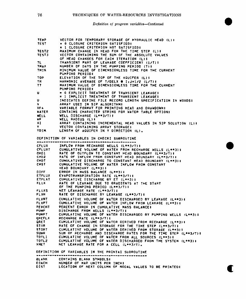
76 TECHNIQUES OF WATER-RESOURCES INVESTIGATIONS
TEHP TEST
TEST2 TfsT3
TL TMAX TMiN
TOP TR TT
U
U V VF4 WATER WELL UP’ XI Y YDIH
Definition of program variables-Continued
VECTOR FOR TEMPORARY STORAGE OF HYDRAULIC HEAD (LlY = 0 CLOSURE CRITERION SATISFIED; = 1 CLOSURE CRITERION NOT SATISFIED: MAXIMUM CHANGE IN HEAD FOR THE TIME STEP (L)I VECTOR CONTAINING THE SUM OF THE ABSOLUTE VALUES OF HEAD CHANGES FOR EACH ITERATION (LlI TRANSIENT PART OF LEAKAGE COEFFICIENT (l/T): NUMBER OF DAYS IN THE PUMPING PERIOD (Tl; MINIMUM VALUE OF DIMENSIONLESS TIME FOR THE CURRENT PUHPING PERIOD: ELEVATION OF THE TOP OF THE AQUIFER (Lit HARMONIC AVERAGE OF T/DELX (D I,J*1/2 (L/T) i MAXIMUM VALUE OF DIMENSIONLESS TIME FOR THE CURRENT PUMPING PERIOD8 = 0 EXPLICIT TREATMENT OF TRANSIENT LEAKAGE: = 1 IMPLICIT TREATMENT OF TRANSIENT LEAKAGE; TNDICATES DEFINE FILE RECORD LENGTH SPECIFICATION IN UORDS; ARRAY USED IN SIP ALGORITHM: VARYABLE FORMAT FOR PRINTING HEAD AND DRAWDOUN; CONTAINS CHARACTER STRING FOR WATER TABLE OPTION; WELL DISCHARGE (L**3/Tl i WELL RADIUS (Ll i ARRAY CONTAINING INCREMENTAL HEAD VALUES IN SIP SOLUTION (Lla VECTOR CONTAINING ARRAY STORAGE: LENGTH OF AQUIFER IN Y DIRECTION (Ll.
DEFINITION OF VARIABLES IN CHECK1 SUBROUTINE -.---------L-III------------------------~--- CFLUX CFLUXT GHDl CHD2 CHDT CHST
OIFF ETFLUX ETFLXT FLUX
FLUXS FLXN FLXNT FLXPT PERCNT PUMP PUMPT QREFLX QRET STOR STORT SUMR TOTL 1 TOTLP XNET
INFLOW FROM RECHARGE WELLS (L**3/Tli CUMULATIVE VOLUME OF WATER FROM RECHARGE WELLS (~**31: RATE OF OUTFLOW TO CONSTANT HEAD BOUNDARY (L-3/T): RATE OF INFLOW FROM CONSTANT HEAD BOUNDARY (L**J/T); CUMULATIVE DISCHARGE TO CONSTANT HEAD BOUNDARY (L**Jlt CUMULATIVE VOLUME OF WATER INFLOW FROM CONSTANT HEAD BOUNDARY (LO*31 i ERROR IN MASS BALANCE (LO*311 EVAPOTRANSPIRATION RATE LL**3/Tl; CUMULATIVE DISCHARGE BY ET (L**31; RATE OF LEAKAGE DUE TO GRADIENTS AT THE START OF THE PUMPING PERIOD (L**3/Tl8 NET LEAKAGE RATE (L**3/Tl; RATE OF DISCHARGE BY LEAKAGE (L**3/Tl1
CUMULATIVE VOLUME OF WATER DISCHARGED BY LEAKAGE (L-31: CUMULATIVE VOLUME OF WATER INFLOW FROM LEAKAGE (L**31; PERCENT ERROR IN CUMULATIVE MASS BALANCE: DISCHARGE FROM WELLS (L**3/T)i CUMULATIVE VOLUME OF WATER DISCHARGED BY PUMPING WELLS tL**3); RECHARGE RATE (L**3/Tlt CUMULATIVE VOLUME OF WATER DERIVED FROM RECHARGE (L**Jl: RATE OF CHANGE IN STORAGE FOR THE TIME STEP (L**3/TlI CUMULATIVE VOLUME OF WATER DERIVED FROM STORAGE (L**311 SUM OF RECHARGE AND DISCHARGE RATES FOR THE TINE STEP (L**3/Tl: CUMULATIVE VOLUME OF WATER FROM ALL SOURCES (L**311 CUMULATIVE VOLUME OF WATER DISCHARGED FROM THE SYSTEM (LO*311 NET LEAKAGE RATE FOR A CELL fL**3/Tl.
DEFINITION OF VARIARLES IN THE PRINTAI SUBROUTINE ----------------------------------------~-------- BLANK CONTAINS BLANK SYHBOLS: DINCH NUM8ER OF MAP UNITS PER INCH: DIST LOCATION OF NEXT COLUMN OF NODAL VALUES TO BE PRINTEDI
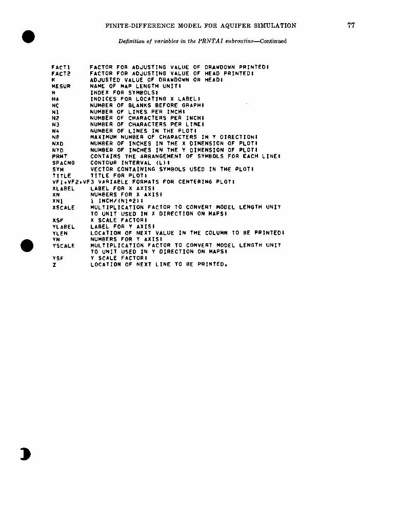
FINITE-DIFFERENCE MODEL FOR AQUIFER SIMULATION 77
FdCTl FACT2 K ME SUR N Na NC Nl N2 N3 N4 Nf! NXD NYD PRNT SPACNG SYM TITLE
Definition of variables in the PRNTAI subroutine-Continued
FACTOR FOR aDJUSTING VALUE OF DRAWDOWN PRINTED: FACTOR FOR ADJUSTING VALUE OF HEAD PRINTED: ADJUSTED VALUE OF DRAWDOWN OR HEAD& NAME OF MAP LENGTH UNIT; INDEX FOR SYMBOLS; INDICES FOR LOCATING X LABEL; NUMBER OF BLaNKS BEFORE GRaPHi NUMBER OF LINES PER INCH! NUMBER OF CHARACTERS PER INCH8 NUM@ER OF CHARACTERS PER LINE; NUMGER OF LINES IN THE PLOT1 MAXIMUM NUMBER OF CHARACTERS IN Y DIRECTION: NUM8ER OF INCHES IN THE X DIMENSION OF PLOT; NUMBER OF INCHES IN THE Y DIMENSION OF PLOT8 CONTAINS THE ARRANGEMENT OF SYMBOLS FOR EACH LINE; CONTOUR INTERVAL (Lb i VECTOR CONTAINING SYMBOLS USED IN THE PLOT; TITLE FOR PLOT8
VFlrVF2rVF3 VPRIAGLE FORMATS FOR CENTERING PLOT: XLaBEL LABEL FOR X AXISI XN NUMBERS FOR X AXIS1 XNl 1 INCH/ (Nl”2) : XSCALE MULTIPLICATION FACTOR TO CONVERT MODEL LENGTH UNIT
TO UNIT USED IN X DIRECTION ON MAPS1 XSF x SCALE FACTOR; YLaREL LABEL FOR Y aXISI YLEN LOCPTION OF NEXT VALUE IN THE COLUMN TO BE PRINTED8 YN NUMBERS FOR Y AXIS; YSCALE HULTIPLICITION FACTOR TO CONVERT MODEL LENGTH UNIT
TO UNIT USED IN Y DIRECTION ON MARSI YSF Z
Y SCaLE FACTOR; LOCATION OF NEXT LINE TO BE PRINTED.
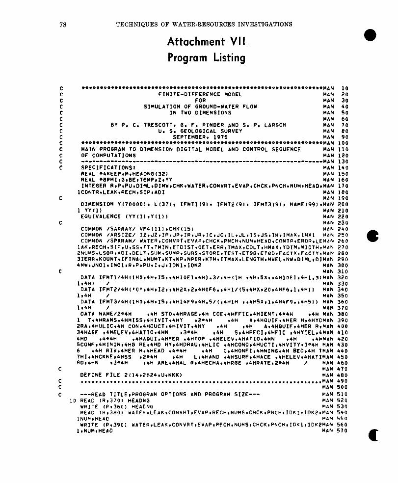
78 TECHNIQUES OF WATER-RESOURCES INVESTIGATIONS
C C C C C C C C
E C
E C
C
C
C
Attachment VII.
Program Listing
OO+OQO00OOOOOOoOOOOOOOOOOOOOOOOOOO~OOOOOOOOOOOOOOOOOOOOOOOOOOO~OOO~~~ 10
FINITE-DIFFERENCE MODEL HbN 20 FOR HbN 30
SIMULATION OF GROUND-WATER FLOW HbN 40 IN TWO DIMENSIONS MAN 50
MAN 60 BY P. C. TRESCOTT, G. F, PINDER AND S. P. LARSON HAN 70
U. So GEOLOGICAL SURVEY MbN 80 SEPTEMBER, 1975 MAN 90
OOOO0O0OO0OOOOOOOO00OOOOOOOOOOOOOOOOOOOOOOOOOOOOOOOOOOOOOOOOOOOOOO~~~ 100 MAIN PROGRAM TO DIMENSION DIGITAL MODEL AND CONTROL SEQUENCE MbN 110 OF COMPUTATIONS MAN 120 ----------------------------------~-------------------------------MAN 130 SPECIFICATIONS, MAN 140 REAL l 4KEEP,M,HEADNG(32) MbN 150 REAL QGPHI,G,GE,TEMP,Z,YY MbN 160 INTEGER RtP,PU,DIML,DIMW,CHK,WATER,CONVRT,EVAP,CHCK,PNCH,NUM,HEAO,MAN 170
lCONTR,LEAK,RECH,SIP,AOI MAN 180 MAN 190
DIMENSION Y(70000)r L(371, IFMTlt9)r IFHTZfP), IFMT3(9), NAME(991,MAN 200 1 YY(l) MAN 210
EQUIVALENCE (YY(l)rYfl)) MAN 220 MAN 230
COMMON /SARRAY/ VF4(ll)rCHK(lS) MAN 240 COMMON /ARSItE/ IZ~JZIIPIJPIIRIJRIICIJC~ILIJLIIS,JS,IH.IMAX,IMX~ MAN 250 COMMON /SPARAM/ WATER,CONVRT,EVAP,CHCK,PNCH,NUM,HEAD,CONTR,EROR,LEMAN 260
1AK,RECH,SIP,U,SS,TT,TMIN,ETOIST,GETtERR,TMAX,C~LT,HMAX,YDIM,WIOTH,M4N 270 ~NUMS*LSOR*ADI,DELT,SUM,SUMP,SURS,STORE~TEST,ETQB,ETQD,FACTX,FAC~Y,MAN 280 3IERR,KOUNT,IFINAL,NUMT,KT,KP,NPER,KTH,ITMAX,LENGTH,NWEL,NW,DIML,DIMAN 290 4MW,JNOl,INOl,R,P,PU,I,J,IOKl,IDK2 MAN 300
MbN 310 DATA IFMT1/4H(1HO,4HrIStr4HlOEl~4Hl.3/,4H(ln r4HrSX,*4HlOElr4H1.3)MAN 320
lr4H) / MAN 330 DATA ~~~~~~~~~~~~~~~~~~~~~~~~~~~~~~~~~~~~~~~~~~~~~~~~~~~~~~~~~~~ MbN 340
1,4H / MAN 350 DATA 1FMT3/4H(1H0,4H,15,,4H14F9,4H.5/~,4H1H ,,4H5X,1,4H4F9.,4H5)) MAN 360
1,4H / MAN 370 DATA NAME/2Q4H ,4H STO,lHRAGE,4H COE,4HFFIC,QHIENT,4Q4H r4H MPN 380
1 T,4HRANS,4HMISS,4HIVIT,4HY r2’4H ,4H A,QHQUIF,4HER H,QHYCMAN 390 2RA,4HULIC,4H CON,4HOUCT,4HIVIT,4HY r4H r4H A,4HQUIF,QHER RtMPN 400 34HASE ,4HELEV,4HATI0,4HN 9 3*4H 94H S,4HPECI,4HFIC ,4HYIEL,4WAN 410 4HO r4Q4H r4HAQUIr4HFER r4HTOP ,4WELEV,4HAT10,4HN r4H r4HNAN 420 SCONF,4HININ,4HG GE,4HO HY,4HORAU,4HLIC ,4tiCONO,4HUCT1,4HVITY,3Q4H MAN 430 6 ,4H RIV,QHER H,4HEAO ,4Q4H r4H C,4HONFI,4HNING,4H GEO,QH THAN 440 7HI,4HCKNE,4HSS ,2*4H r4H L,4HAND ,4HSURF,4HACE ,4HELEV,SHATIMAN 450 GOt4HN ,3*4H r4H ARE,4HAL R,QHECHA,4HRGE ,4HRATE,2*4H / MAN 460
MAN 470 DEFINE FILE 2(14,2624,U,KKK) MAN 4GO . . . . . . . . . . . . . . . . . . . . . . . . . . . . . . . . . . . . . . . . . . . . . . . . . . . . . . . . . . . . . . . . . . MbN 490
HAN 500 ---READ TITLE,PROGRAM OPTIONS AND PROGRAM SIZE--- MAN 510
10 READ (R,370) HEADNG MAN 520 WRITE (P,360) HEAONG MAN 530 READ (I?,3801 WATER,LEAK,CONVRT,EVAP,R~CH,NUMS,CHCK,PNCH,IDKl,I~K2,MAN 540
lNUM,HEAO MAN 550 WRITE (Pt390) WATER,LEAK,CONVRT,EVAP,R~CH,NUMS,CHCK,PNCH,IDKl,IDK2~AN 560
l,NUM,HEAD MAN 570
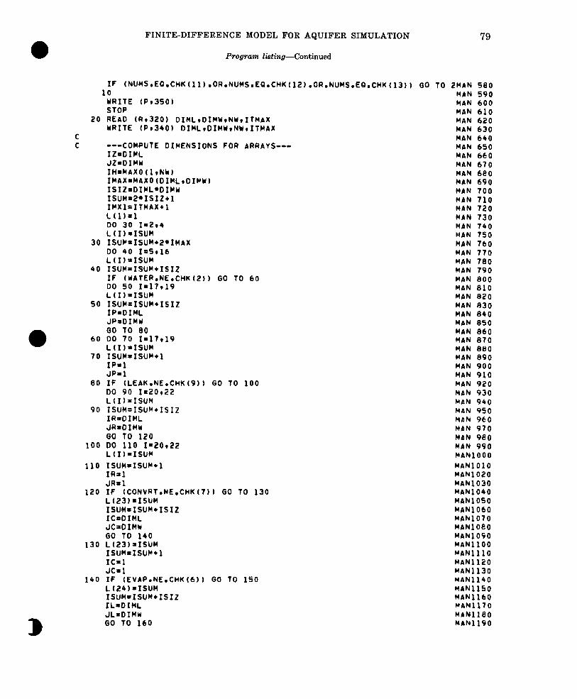
FINITE-DIFFERENCE MODEL FOR AQUIFER SIMULATION
Program listing-Continued
IF (NUHS.EG.CHK(ll).DR.NUMS.EQ.CHK(l2~.OR.NUMS.EQ.CHK~l3)~ GO TD 2MAN 500 10 MAN 590
WRITE (Pe3501 MAN 600 STOP MAN 610
20 READ (R1320) DIML~DIMW~NW~ITMAX MAN 620 WRITE (Pv340) DIML~DIWW~NW,1TMAX MAN 630
C MAN 640 C ---COMPUTE DIMENSIONS FOR ARRAYS--- MAN 650
IZ=DIHL MAN 660 JZ=DIMW MAN 670 IH=MAXO(lrNk) MAN 680 IMAX=MAXO(DIHLIDILW) MAN 690 ISIt~DIWL*DIMw MAN 700 ISUM=E*ISIZ+l MAN 710 IMXl=ITNAX*l MAN 720 L(l)=1 MAN 730 DO 30 11214 MAN 740 L(I)=ISUM MAN 750
30 ISUY=1SUM*2*1MAX MAN 760 DO 40 I=5916 MAN 770 L(I)=ISUM MAN 780
40 ISUM=ISUM*ISIZ NAN 790 IF (WATER.NE.CHK(E)) GO TO 60 MAN 800 DO 50 X=l?rl9 MAN 810 L(I)=ISuM MAN 820
50 ISUH=ISUM*ISIZ MAN 830 IP=DIML MAN 840 JPIDIMW MAN 050 GO TO 80 MAN 860
60 DO 70 1=17rl9 MAN 070 L(I)=ISUM MAN 880
70 ISUMoISUM+l MAN 890 IP=l MAN 900 JP=l MAN 910
80 IF (LEAK.NE.CHK(9)) GO TO 100 MAN 920 DO 90 1~20922 MAN 930 L(I)=ISUH MAN 940
90 ISUH=ISUM*ISIi! MAN 950 IR=DIML MAN 960 JR=DIMW MAN 970 GO TO 120 MAN 980
100 DO 110 1'2Oe22 MAN 990 L(I)=ISUM MAN1000
110 ISUM=ISUM*l MAN1010 IR=l MAN1020 JR=1 MAN1030
120 IF (CONVRT.NE.CHK(7)l GO TO 130 MAN1040 L(23)-ISUM MAN1050 ISUM=ISUM*ISIZ MAN1060 IC*DIML MAN1070 JC=OIMW MAN1080 GO TO 140 MAN1090
130 L(23)=ISUM MAN1100 ISW=ISUM*l MAN1110 IC=l MAN1120 JC=l MAN1130
140 IF (EVAP.NE.CHK(6)) GO TO 150 MAN1140 L(24)=ISUM MAN1150 ISUM=ISUM+ISIZ MAN1160 IL=DIML MAN1170 JL=DIMw MAN1180 GO TO 160 HAN1190
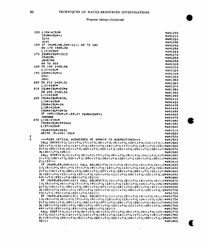
80 TECHNIQUES OF WATER-RESOURCES INVESTIGATIONS
Program listing--Continued
32))) MAN1800
a
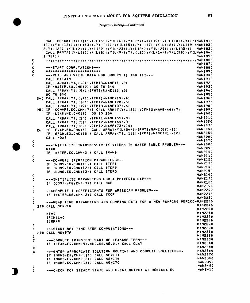
FINITE-DIFFERENCE MODEL FOR AQUIFER SIMULATION 81
Program listing--Continued
CALL CHECKI~Y~L~l~~rY(L~S~~,Y~L~6~~rY~L~7~~rY~L~9~~,Y(L(lO~)~Y(L~lMANl8lO ~~~~~~~~~~~~~~~~~~~~~~~~~~~~~~~~~~~~~~~~~~~~~~~~~~~~~~~~~~~~~~~~~~~~~~~~~~ ~~~~~~~~~~~~~~~~~~~~~~~~~~~~~~~~~~~~~~~~~~~~~~~~~~~~~~~~~~~~~~~~~ MAN1830
CALL PRNTAI(Y~L~l))rY~L(B)~~Y~L(9))rY(L~12)~,Y~L~l4~~,Y~L(29~~~Y~LMANl640 l(32))) MAN1850
C . . . . . . . . . . . . . . . . . . . . . . . . . . . . . . . . . . . . . . . . . . . . . . . . . . . . . . . . . . . . . . . . . . MAN1860
z ---START COMPUTATIONS---
E 0~*~9*0+*10*010904,0~**~ ---READ AND WRITE DATA FOR GROUPS II AND III--- CALL DATAIN CALL ARRAY(Y~L(l2))rIFHT3rNIHEor2) IF tWATER.EQ.CHK(2)) GO TO 240 CALL ARRAY(Y(L(9))rIFMT3rNAHE(lO)r3) GO TO 250
240 CALL ARRAY(Y(L(17))rIFMTlrNAME(19)e4) CALL ARRAY(Y(L(lG))rIFMT2rNAME(28)rS) CALL ARRAY(Y(L(lP))tIFMT3(NIHE(37B~6f
250 IF (CONVRT.EQ.CWKt7)) CALL ARRAY(Y(L(23))rIFMTZvNAME(46lv71 IF (LEAK.NE.CHK(9)) GO TO 260 CALL ARRAY(Y(L(ZO~)rIFMTl~NAHE~55),8) CALL ARRAY(Y(L(21)),IFHT2rNAHE(64)*9) CALL ARRAYtY(L(22))tIFMT2rNAME(73)*10)
260 IF (EVAP.EQ.CHK(6)) CALL ARRAY(YfL(24))rIFMT2rNAME(82)tlL) IF (RECH.EQ.CHK(lO)) CALL ARRAY(Y(L(l3)),IFMTl(NPHE(9l)rlZ) CALL MOAT
---INITIALIZE TRANSMISSIVITY VALUES IN WATER TABLE.PROBLEM--- KT-0 IF (WATER.EQ.CHK(Z)) CALL TRANS
C C ---COMPUTE ITERATION PARAMETERS---
IF fNUMS.EQ.CHK(ll)) CALL ITERl IF (NUMS.EQ.CHK(lZ)) CALL ITERE IF (NUMS.EQ.CHK(13)) CALL ITERJ
C C ---INITIALIZE PARAMETERS FOR ALPHAMERIC HAP---
IF (CONTR.EQ.CHK(3)) CALL MAP C C ---COMPUTE T COEFFICIENTS FOR ARTESIAN PROBLEM---
IF tWATER.NE.CHK(Z)) CALL TCOF
MAN1070 MANlBGO MAN1890 MAN1900 HAN1910 MAN1920 MAN1930 MAN1940 MAN1950 HAN1960 MAN1970 MPN19GO MAN1990 MAN2000 MAN2010 MAN2020 MAN2030 MAN2040 MPN2050 MAN2060 MAN2070 MAN2080 MAN2090 MAN2100 MAN2110 MAN2120 MAN2130 MAN2140 MAN2150 MAN2160 MAN2170 MAN2180 MAN2190 MAN2200 MAN2210
C MAN2220 C ---READ TIME PARAMETERS AND PUMPING DATA FOR A NEW PUMPING PERIOD-MAN2230
270 CALL NEWPER MAN2240 C MAN2250
KT=O MAN2260 IFINALmO MPN22?0 IERR= MAN2280
C MAN2290 C ---START NEW TIME STEP COMPUTATIONS--- MbN2300
280 CALL NEWSTP MAN2310 C MAN2320 C ---COMPUTE TRANSIENT PART OF LEAKAGE TERM--- MAN2330
IF (LEAK.EQrCHK(P).AND.SS.NE.O.) CALL CLAY MAN2340 C MAN2350 C -?--ENTER APPROPIATE SOLUTION ROUTINE AN0 COMPUTE SOLUTION--- MAN2360
IF (NUMS.EQ.CHKtll)) CALL NEWITA MAN2370 IF (NUMS.EQ.CHK(lZ)) CALL NEWITG HAN2380 IF tNUHS.EQ.CHKf13)) CALL NEWITC MAN2390
C MAN2400 C ---CHECK FOR STEADY STATE AND PRINT OUTPUT AT DESIGNATED MAN2410
82 TECHNIQUES OF WATER-RESOURCES INVESTIGATIONS
Program list&g-Continued
C TIME STEPS--- MAN2420 CALL STEADY MAN2430
e MAN2440 C ---LAST TIME STEP IN PUMPING PER100 ?--- MAN2450
IF IfFINAL.NE.1) GO TO EGO MAN2460 C MAN2470 C ---CHECK FOR NEW PUMPING PERIOD--- MAN2480
IF (KP.LT.NPER) GO TO 270 MAN2490 C MPN2500 C ---DISk OUTPUT IF DESIRED--- MAN2510
IF (IDKZ.NE.CHK(l51) GO TO 290 MAN2520 tALL DISK MbN2530
E MAN2540
---PUNCHED OUTPUT IF DESIRED--- MAN2550 290 IF (PNCH.,NE.CHK(l) 1 GO TO 300 MAN2560
CALL PUNCH MAN2570 C MAN2580 C --4CHECK FOR NEW PROBLEM--- MAN2590
300 READ (R’320rEND=3101 NEXT MAN2600 IF (NEXT.EQ.01 GO TO 10 MAN2610
310 STOP MAN2620 C . . . . . . . . . . . . . . . . . . . . . . . . . . . . . . . . . . . . . . . . . . . . . . . . . . . . . . . . . . . . . . . . . . MAN2630 C MAN264 0 C ---FORMATS--- MAN2650 C ,,,,,,,,-,,,,,,,,,--,,---------• ------~-------------------------------MAN~~~O C MAN2670 C MAN2680
320 FORMAT (41101 MAN2690 330 FORMAT (‘O’r54Xv’WORDS OF Y VECTOR USED =“I71 MAN2700 340 FORMAT (‘0”62X,‘NUMBER OF ROWS =“15/60X”NUMBER OF COLUMNS =‘rISMAN2710
1/9X.*NUWBER OF WELLS FOR WHICH DRALrOObN IS COMPUTED AT A SPECIFIECMAN2720 2 RADIUS =“15’/‘39X”HAXIMUM PERMITTED NUMBER OF ITERATIONS =“15)MAN2730
350 FORMAT (‘0”36X”NO EQUATION SOLVING SCHEME SPECIFIED’ EXECUTION tMAN2740 lERMINATED’/37X’58(‘*‘11 MAN2750
360 FORMAT (‘l’r6OX”U. S. G. S.‘//SSX”FINITE-DIFFERENCE MODEL’/65X”MAN2760 1FOR’/51X”SICULATION OF GROUND-WATER FLOW’//60X”JANUARY’ 1975'//1MAN2770 233~'*0/'0'~32A4//1330) MAN2780
370 FORMAT (2OA41 MAN2790 300 FORMAT (16(A4rlX11 MAN2800 390 FORMAT (‘-SIMULATION OPTIONS1 't13(A4*4X)) MAN2610
END MANZBZO-
SUBROUTINE OATA~~PHI.STRT~SU~I~trTRITC,S’QRE.WELL’lL’SL~PERM’GOTlCDAT 10 1MtSY’RATE’RIVER’H’TOP’GRND’OELXiDELY’WR’NWR~ DAT 20
---------------------------I-------------------------------- --------,,,,T 30 READ AN0 WRITE INPUT OATA OAT 40 ,,,,,,;,--,.-,,---------------------------------------------------DAT 50
DAT 60 SPECIFICATIONS1 OAT 70 REAL *GPHI’OBLE~XLABEL’YLABEL’lIlLE’XNlrMESUR OAT GO REAL *4M DAT 90 INTEGER R’P’PU’DIKL’DIMW’CHK’WATER’CONVRT,EVAP’CHCK~PNCH’NUM~HEAO’OAT 100
lCONTR’LEAK’RECHrSIP’AD1 OAT 110 DAT 120
OIHENSION PHI(IZ’JZ1’ STRT(IZIJZ)’ SURI~IZIJZ)’ T(IZ’JZ1’ TRfIZ’JZOAT 130 1)’ TC(IZ’JZ1’ S(IZ’JZ)r BRE(I2’JZ) ’ WELL11Z’JZ)r TL(IZ’JZ1’ SL(IZrDAT 140 2JZ)r PERM(IP*JP)* BOTTOM(IPeJP)r SY(IPIJP)~ RATE(IReJR)r RIVER(IR’OAT 150 3JR1’ M(IR’JR)* TOP(IC’JC)r GRND(IL’JL1’ DELX(JZ1’ DELY(IZ1’ WR(ICoDAT 160 4’ NWR(IH’21, A(IZ’JZ1’ IN(Q)’ IFMT(91 DAT 170
DAT 180
C C
C C C
C C
0
C C C C
C
C
B
FINITE-DIFFERENCE MODEL FOR AQUIFER SIMULATION 83
Program listing-Continued
COMMON /SARRAY/ VF4(1lbgCHK(lS) CAT 190 COMMON /SPARAY/ ~ATERICONVRTIEVAPICHCK~PNCH~NUMIHEADICONTR*FROR*LECAT 200
1AK~RECH~SIP~U,SS~TT,TYINIETOISTtOETtERR~TMAX~CCLT~HMAX~YCIM~WICTH~CAT 210 ~NUMSILSOR~ACI~CELTISUM~SUMP~SUES~STORE~TEST~ETQ~~ETQC~FACTX,FACTY~CAT 220 3IERR,KOUNTtIFINAL~NUMT~KT~KPINPER~KTH~ITMAX~LENGTH~NWEL~N~~@IML~CICAT 230 4MY~JNOlrINOlrRtP~PU,IIJtIDKlrIDK2 CAT 240
COMMON /CK/ ETFLXTISTORTIQRETICWSTICHO~~PLUXT~PUMPT~CFLUXT~FLXNT CAT 250 COMMON /PR/ XLABEL(3)rYLABEL(6)rTITLE(5)~XNlrMESUR~PRNT~l22)*BLANKCAT 260
1f60~~CIGIT~l22~tVF1~6~~VF2~6~~VF3~7~~XSCALE~DINCH~SYM~l7~~XN~lOO~~CAT 270 2YN(l3)rNAt4)rNlqNZ~N3rYSCALEtFACTlvFACT2 DAT 280
COMMON /ARSIZE/ IZ~JZ~IP*JP~IR~JR~IC~JCIILIJL~IS~JS~IHIIMAX~IMX~ CAT 290 RETURN CAT 300 . . . . . . . . . . . . . . . . . . . . . . . . . . . . . . . . . . ..*...*......................... CAT 310 l *******+******4ft*+* CAT 320 ENTRY OATAIN CAT 330 0*********it4******** CAT 340
CAT 350 ---READ AN0 WRITE SCALAR PARAMETERS--- PAT 360 READ (ReSOO) CONTR,XSCALEIYSCALEICINCH~FACT~~FACT~~MESUR OAT 370 IF (CONTR.EQ.CHKt3)) WRITE (P1610) XSCALE.YSCALE.MESUR.MESURIDINCHbAT 380
lrFACTlrFACT2 CAT 390 READ fRe490) NPERIKTH~ERR~ERORISS~QE~~ET~ETCIST~LENGTH~H~AX~FACTX~FACCAT 400
1TY CAT 410 IF (ETCIST.LE.0,) ETCISTel. CAT 420 WRITE fPt520) NPERIKTH~ERR~ERORISSIQETIET~ETCIST~FACTX~FACTY CAT 430
CAT 440 ---READ CUMULATIVE MASS BALANCE PARAMETERS--- CAT 450 READ (Rq600) SUMISUMPIPUMPT~CFLUXTIQRETICHSTICHDTIFLUXT~STORT~ETFLCAT 460
1XTeFLXNT CAT 470 IF (ICKl.EQ.CHK(14)) GO TO 20 CAT 480 IF (SUM.EQ.0.o) GO TO 40 CAT 490 WRITE (P*480) SUM CAT 500 . . . . . . . . . . . . . . . . . . . . . . . . . . . . . . . . . . . . . . . . . . . . . . . . . . . . . . . . . . . . . . . . . . OAT 510
CAT 520 ---HEAD DATA TO CONTINUE PREVIOUS COMPUTATIONS READ HERE--- CAT 530 ------FROM CARDS: CAT 540 CO 10 I=ltDIML OAT 550 REAU (Rt540) (PHI(IrJ)~J=ltCIMW) DAT 560
10 WliITE (P1530) 1~ (PHI (IIJ) tJ=lrCIMW) CAT 570 GO TO 40 DAT 5.90 ------READ AND lrrRITE DATA FROM UNIT 4 ON DISK RATHER THAN CARDS: DAT s(;o
20 READ (4) PHIISUMISUMP~PUMPT~CFLUXT~QRETIC~STICHDT~FLUXT~STDRT~ETFLDAT 600 lXT,FLXNT CAT 610
kRITE fP1480) SUM DAT 620 DO 30 I=l.DIML DAT 630
30 ‘kR1TE (P*530) II (PHI (I,J) rJ=lrCIMk) CAT 640 REWIND 4 CAT 650 . . . . . . . . . . . . . . . . . . . . . . . . . . . . . . . . STRT (STARTIhG HEAD) . . . . . . . . . . . . DAT 660
40 READ (Ff1490) FACT~IVARIIPRN~IRECS~IRECD CAT 670 IF (lHECS.EQ.l) READ (2’1) STRT D4T 680 IF ((IVAR.EP.1.OR.IRECS.EQ.l~.ANl-J.IPRN.NE.1~ lrRITE (P1470) CAT 690 CO 80 I=lrCIML CAT 700 IF (IVAR.EQ.l) READ (Rt540) (STRT(IIJ)~J=~~CIMW) CAT 710 CO 70 J=lrDIPC CAT 720 IF (IRECS.EO.l) GO TO 60 CAT 730 IF (IVAR.NE.l) GO TO 50 CAT 740 STRT(IIJ)=STRT(I~J)QFACT CAT 750 GO TO 60 DAT 760
50 STRT(IeJ)=FACT OAT 770 CO SURI(IIJ)=STRT(IIJ) CAT 7@0
T(I*J)=O. PAT 785
84 TECHNIQUES OF WATER-RESOURCES INVESTIGATIONS
Program listing--Continued
TL(I,J)=O. SL(IvJ)=O. TR(IeJ)=O. TC(I*J)=O. bELL(IvJ)=O.O QRE(IrJ)=O.
70 TF (SUM.EQ.O.O.AND.IDKl.NE.CHK(14)) P~I(IIJ)=STRT(I*J) IF (IVAH.EO.O.ANO.IRECS.EQ.O.~R.IPRN.EQ.l) GO TO 80 WGITE (Pq530) I~(STRT(IIJ)~J=~~DIMW)
PO CCNTINUE IF (IVAR.hE.l.AND.IRECS.NE.1~ WRITE (Pq420) FACT IF (IRECD.EQ.l) WRITE (2'1) STRT RETURN
C C ---READ REMAIhING ARRAYS FROM CARDS OR DISK (AS SPECIFIED IN THE C .OPTIONS) AND WRITE THEM ON DISK IF SPECIFIED IN THE OPTJONS--- C it*itoof+4*o**oo*
EhTRY ARRAY(AIIFMTIINIIRN) C oo******o4+4t4to4
READ (Rq490) FACTIIVARIIPRN~IRECS~IRECD IK=4*IRECS*2"IVAR+IPRN+l GO TO (90r90t110t110~140~140~~ IK
90 DO 100 I=ltDIHL DO 100 JalrOIMW
100 AfIrJ)=FACT WRITE (P1430) INeFACT 80 TO 160
110 IF (IK.EQ.3) WRITE (P1440) IN DO 130 I=lrOIHL READ (R1510) (A(I,J)rJ=ltDIMW) DO 120 J'l~OIHW
126 A(IIJ)=A(IIJ)*FACT 130 IF (IK.EQ.3) YRITE (PtIFMT) IefAtItJ)rJ=lrDIMW)
GO TO 160 140 READ (Z*IRN) A
IF (IK.EQ.6) GO TO 160 WRITE IP1440) IN DO 150 I=lqDIML
150 WRITE (PtIFHT) Ir(A(ttJ)tJ=lrDIHW) 160 IF (IRECD.EQ.1) WRITE (2tIRN) A
RETURN C C ---INSERT ZERO VALUES IN THE 1 OR PERM MATRIX AROUND THE C BORDER OF THE MODEL--- C 44**********4*
ENTRY MOAT C ***a**********
DO 180 I'lrlJIML DO 180 J=lrOIMW IF (WATER.EQ,CHK(Z)l GO TO 170 IF (I.EQ~1.OR.I.EQ.DIHL.OR.J.EQ.l.OR.J.EQ.DIMU~ T(I+J)=O.
DAT 790 DAT 800 DAT 810 OAT 820 DAT 830 DAT 840 DAT 850 DAT 860 OAT 870 DAT 880 DAT 890 DAT 900 DAT 910 DAT 920 DAT 930 DAT 940 OAT 950 DAT 960 DAT 970 DAT 980 OAT 990 OAT1000
DATlOlO OAT1020 OAT1030 DAT1040 OAT1050 DAT1060 DAT1070 DAT1080 DATlO90 DATllOO OAT1110 DATll20 DAT1130 DAT1140 OAT1 150 OAT1160 DA11170 DATll@O DAT1190 DAT1200 DA71210 DAT1220 CAT1230 OAT1240 DAT1250 OAT1260 OAT1270 DAT1280 DAT1290
GO TO 180 DAT1300 170 IF (I.EQ~l.OR.I.EQ.OIML.OR~J.EQ.l.OR.J.EQ.DIMW~ PERHfI,J)=O. DAT1310 180 CONTINUE DAT1320
C . . . . . . . . . . . . . . . . . . . . . . . . . . . . . . . . DELXIOELY . . . . . . . . . . . . . . . . . . . . . ..DATl330 READ (Rt490) FACT~IVARIIPRN~IRECSWIRECD DAT1340 IF fIRECS.EC.1) GO TO 210 DAf1350 IF fIVAR.EQ.1) READ (Re490) DELX DATl360 DO 200 J=lrCIMW DAT1370 IF (IVAR.NE.l) GO TO 190 DAT1380 DELX(J)=DELX(J)*FACT DAT1390
FINITE-DIFFERENCE MODEL FOR AQUIFER SIMULATION
Program listing-Continued
GO TO 200 190 DELX(J)=FACT 200 CONTINUE
GO TO 220 210 READ (2'13) DELX 220 IF (1RECD.EQ.I) WRITE (2'13) DELX
IF ~IVAR.EQ.l.OR.IRECS.EQ.l.AND.IPRN.NE.1) WRITE (P1550) OELx IF (1VAR.NE.l.AND.IRECS.NE.l) WRITE (Pe450) FACT READ (Re4901 FACT,IVARIIPRNIXRECSIIRECD IF (IRECS.EQ.1) GO TO 250 IF (IVAR.EQ.l) READ (Rv490) DELY
DO 240 I=lrOXML IF (XVAR.NE.1) GO TO 230 DELY(I)=DELY(I)*FACT GO TO 240
230 DELY(X)=FACT 240 CONTINUE
GO TO 260 250 READ (2'14) DELY 260 IF (XRECD.EQ.l) WRIT
IF (IVAR.EQ.l.OR.IRE IF (XVAR.NE.~.ANDIXR
C
E (2'14) DELY CS.EQ.l.AND.IPRN.NE.1) WRITE (Pv560) DELY ECS.NE.1) WRITE (Pv460) FACT
C ---INITIALIZE VARIABLES--- JNOl=DIMW-1 INOl=OXML-1 IF (LEAK.NE.CHK(9).0R.SS.NE.O.) GO TO 280 00 270 1=211NOl DO 270 J=2rJNOl IF (M(IvJ).EQ.O.) GO TO 270 TL~X~J)=RATE~XIJ)/M(X~J)
270 CONTINUE 280 ETQB=O.O
ETQO=O.O SUBS=O.O WlrO TTnO.0 XM=WIN0~6*DIHW~4rl24~ XM=(132-IM)/2 VF4(3)+DIGXT(IMb VF4(B~=DIGXT(IM*S~ WIDTkirO. DO 290 J=2rJNOl
290 WIDTH~WIDTH*DELX~J~ YDIN=O. 00 300 1=211NOl
300 YDIN=YOI~*OELY~I~ RETURN
OAT1400 OAT1410 OAT1420 OAT1430 OAT1440 DAT1450 OAT1460 OAT1470 DA11480 OAT1490 OAT1500 OAT1510 OAT1520 DAT1530 OAT1540 OAT1550 OAT1560 OAT1570 OAT1580 OAT1590 OAT1600 OAT1610 OAT1620 DAT1630 OAT1640 OAT1650 OAT1660 OAT1670 DATl660 OAT1690 DAT1700 DAT1710 DAT1720 DAT1730 OAT1740 OAT1750 OAT1760 DAT1770 OAT1780 DATl790 OAT1800 DATl810 OAT1820 oATl830 OAT1840 DA11850 DA11860 OAT1870 -
C . . . . . . . . . . . . . . . . . . . . . . . . . . . . . . . . . . . . . . . . . . . . . . . . . . . . . . . . . . ..o~....~ATl880 C OAT1890 C ---READ TIME PARAMETERS AND PUMPING DATA FOR A NEW PUMPING PERIOD-DAT1900 C O*~a~*OI*OI*~*~O*QO~OQO* DAT1910
ENTRY NEWPEA DAT1920 C •4QQQIO~*OQI~QQI~*~~*~*~ OAT1930 C DAT1940
READ (Ra490) KPIKPM~~NWELITMAXINUMT~COLTIDELT~DELT OAT1950 C OAT1960 C ---COMPUTE ACTUAL DELT AND NUt'tT--0 OAT1970
DT=DELT/24. DAT1980 TM=O.O DAT1990 DO 310 I=lrNUHT OAT2000
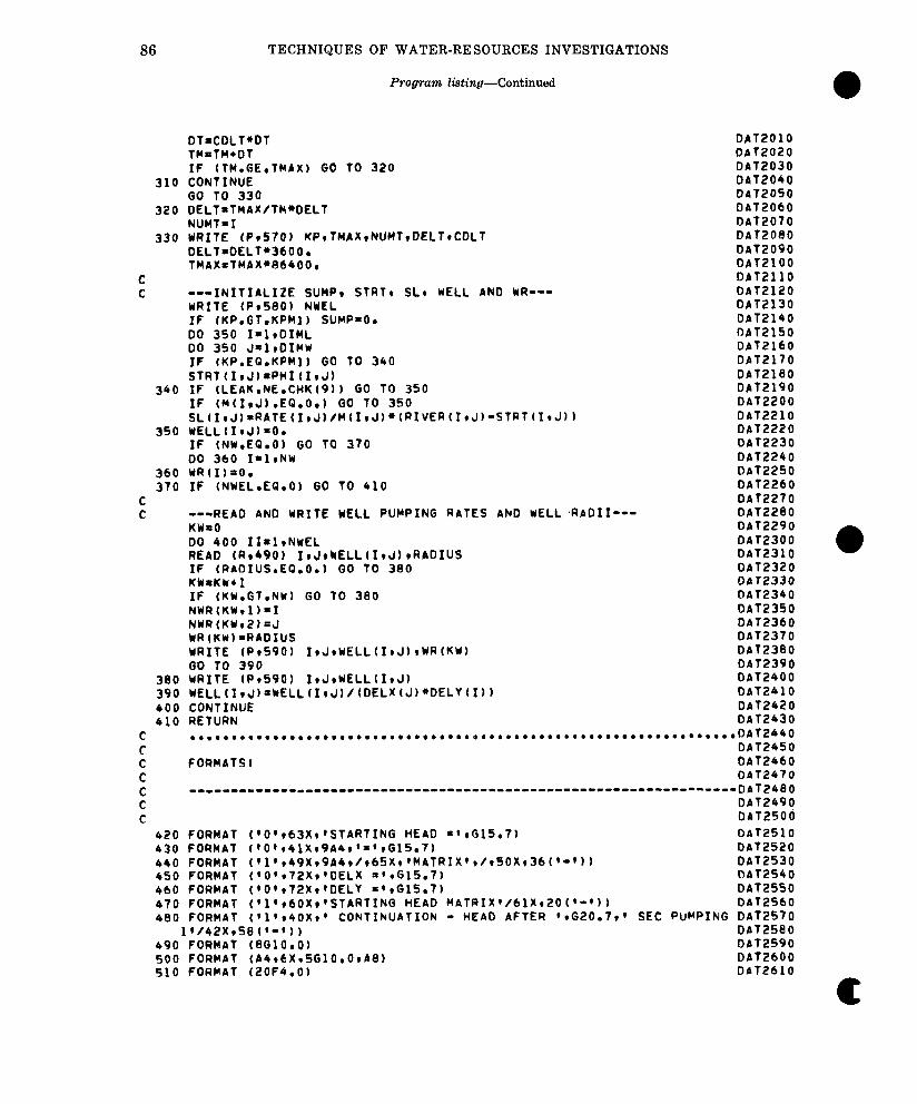
86 TECHNIQUES OF WATER-RESOURCES INVESTIGATIONS
310
320
330
C C
340
350
360 370
C C
300 390 400 410
C C
z
: C
420 430 440 450 460 470 480
Program Ming-Continued
DT=CDLT*Df THnTH+DT IF (fM.GE.TMAx) GO TO 320 CONTINUE GO TO 330 DELT=THAX/TM*DELT NUMT=I WRITE (P’570) KP’TMAX’NUMT’DELT’CDLT DELT=DELT*3600. TMAX=THAX*86400.
---INITIALIZE SUMP’ STRT’ SL’ WELL AND WR--- WRITE (P’S801 NWEL IF IKP.GT.KPHl) SUMP=O. DO 350 I=l’DIML DO 350 J=l’DIHW IF fKP,EQ,KPMl) GO TO 340 STRT(I’J)=PHI(I’J) IF (LEAK.NE,CHK(Q)) GO TO 350 IF (M(I’J).EQ.O.) GO TO 350 SL~I’J~~RATE~I’J~/M(I’J)*(RIVER(IIJ)-STRTtI’Ji) WELLfI’J)=O.
OAT2010 OAT2020 OAT2030 DA12040 OAT2050 OAT2060 OAT2070 OAT2000 OAT2090 OAT2100 OAT2110 DATE120 OAT2130 OAT2140 OAT2150 OAT2160 OAT2170 OAT2180 OAT2190
IF (NW.EQ.0) GO TO 370 DO 360 I'l'NY WR(I)rO. IF (NWEL.EQ.0) GO TO 410
---READ AND WRITE WELL PUMPING RATES AND WELL,RPDII--- KU-0 DO 400 II~l'NwEL READ fR’490) I’J’~ELL(I’J~‘RADIUS IF (RAOIUS.EQ.0.) GO TO 300 KWoKN* 1 IF (KW.GT.NW) GO TO 380 NWR~KW’l)=I NWR(KW’2)=J WRfKW)=RADIUS WRITE fPt590) I’J’WELLfI’J) ‘WRfKW) GO TO 390 WRITE (P’590) I’J’WELL(I’J) WELL(I’J~=CELL(I’J)/(DELX(J)*DELY~X)) CONTINUE RETURN
OAT2200 OAT2210 OAT2220 OAT2230 OAT2240 OAT2250 OAT2260 OAT2270 OAT2260 OAT2290 OAT2300 OAT2310 OAT2320 DA 72330 OAT2340 OAT2350 DA72360 OAT2370 OAT2300 DA12390 OAT2400 DOT2410 OAT2420 OAT2430
. . . . . . . . . . . . . . . . . . . . . . . . . . . . . . . . ..*............................... DAT2440 OAT2450
FORMATS I OAT2460 OAT24?0
~~-~~~-II--------~--~~~~~~~~~~~~~~~~~~~~~~~~~~~~~~~~~~~~~~~~~~~~~~ OAT2400 DbT2490 OAT2506
FORMAT (‘O”63X”STbRTING HEAD n”G15.7) OAT2510 FORMAT ~'O"41X'9A4"="G15.7~ DAT2520 FORMAT (‘1”49X’964’/‘65X”MATR1X”/‘50X’36~’-’~1 OAT2530 FORMAT (‘O”72X”OELX =“G15.7) DbT2540 FORMAT f’O”72X”OELY =“G15.7) OAT2550 FORMAT (‘l”60X”STARTING HEAD MATRIX’/6lX’20(‘-0) ObT2560 FORMAT (‘l”40X” CONTINUATION - HEAD AFTER “620.7” SEC PUMPING OAT2570 - ----- 1*/42X*58(*-0) ObT25eO
490 FORMbT (8GlO.O) DbT2590 500 FORMAT ~A4'6X'5010.0'68) OAT2600 510 FORMAT (20F4.0) OAT2610
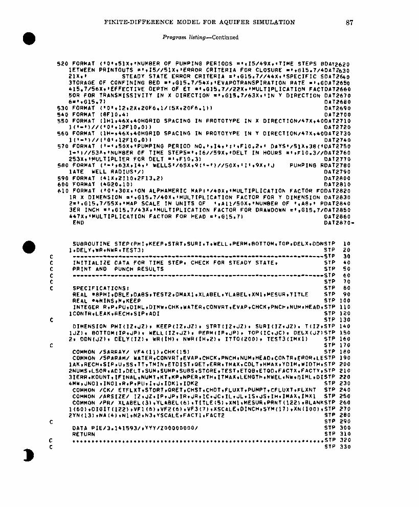
FINITE-DIFFERENCE MODEL FOR AQUIFER SIMULATION
Program listing-Continued
87
C
C
520 FORMAT (‘O**SlX**NUMBER OF PUMPING PERIODS =**15/49X**TIME STEPS GOAT2620 1ETWEEN PRINTOUTS n’eI5//51Xq’ERROR CRITERIA FOR CLOSURE P*rG15.7/4DAT?tf,30 21X*’ STEADY STATE ERROR CRITERIA =‘~G~S.~//QQXI*SPECIFIC SDA12640 3TORAGE OF CONFINING BED =‘*Gl5.7/54X*‘EVAPOTRANSPIRATION RATE =*,GDAT265G 415.7/56X*‘EFFECTIVE DEPTH OF ET ~‘*Gl5.7//22X*‘MULTIPLICATION FACTDAT2660 50R FOR TRANSNISSIVITY IN X DIRECTION =‘rG15.7/63Xe*IN Y DIRECTION OAT2670 6=‘*615.7) DAT2600
530 FORMAT (‘O’eIZv2X,20F6.1/(5Xe2OF6.1)) DAT2690 540 FORMAT (GF10.4) DAT2700 550 FORMAT ~lH1~46X~40HGRID SPACING IN PROTOTYPE IN X DIRECTION/47X*40DAT2710
1~‘~‘)//(‘0’*12FlO*O~~ OAT2720 560 FORMAT (lH-*46X*40HGRID SPACING IN PROTOTYPE IN Y DIRECTION/47X*4ODAT2730
I(‘-‘)//(‘0’*12FlO.O)) OAT2740 570 FORMAT f’-‘*SOX**PUHPING PERIOD NO.**I4t*;‘*FlO.Z** DAYS*/51X*3G(*DAT2750
1~‘)//53X*‘NUMBER OF TIME STEPS=‘*I6//59X**DELT IN HOURS =**FlO.J//DAT2760 253X**MULTIPLIER FOR DELI “rF10.3) OAT2770
580 FORMAT (‘-‘*63X*14* ’ NELLS’/65X*9(‘-0//5OX*‘I’*9X**J PUMPING RDAT2780 1ATE WELL RADIUS’/) DAT2790
590 FORMAT (41X*2110*2F13.2) OAT2800 600 FORMAT (4G20.10) DAT2810 610 FORMAT (‘0’*30X**ON ALPHAMERIC MAPI*/40X**MULTIPLICATION FACTOR FODAT2820
1R X DIMENSION r**G15.7/40X*‘MULTIPLICATION FACTOR FOR Y DIMENSION DAT2830 2=‘*G15,7/55X**MAP SCALE IN UNITS OF ‘rAll/50X*‘NUMBER OF ‘*AG** PDAT2840 3ER INCH =**G15.7/43X*‘MULTIPLICATION FACTOR FOR DAAWDOWN =‘,G15.7/DAT2850 447X**MULTIPLICATION FACTOR FOR HEAD =‘*G15.7) DAT2860
END DAT2870-
SUBROUTINE STEP~PHIIKEEPISTRTISURIIT~~ELLIPERH,BOTTOM,TOP~DELX~DDNSTP 10 ~~DELYIWR~NWA~TEST~) STP 20
--------~--.---~--------------------------------~-----------------STp 30 INITIALIZE CATA FOR TIME STEPI CHECK FOR STEAOY STATE* STP 40 PRINT AND PUNCH RESULTS STP 50 --,-,--------,,--,------------------------------------------------STp 450
STP 70 SPECIFICATIONS! STP 80 REAL ~6PHI~DBLE~DABS~TEST2rDnAXlrXLdBELIYLABEL~YLABEL~XNl~MESUR~TITLE STP 90 REAL “4MINSvMwKEEP STP 100 INTEGER RIPIPU~DIMLIDIMW~CHK~YPTERICONVRT,EVAPICHCK~PNCH~NUM*HEAD~STP 110
1CONTReLEAKtRECHrSIPtADl STP 120 STP 130
DIMENSION PHI(IZrJZ)r KEEP(IZ,JZ)r STRT(IZeJZ)r SURItIZeJZ)r TtIZtSTP 140 1JZ)r GOTTOM~IPIJP)~ WFLL~IZIJZ)~ PERM(IP*JP)r TOP(ICIJC)* DELX(JZ)STP 150 21 DDNtJZ)e CELY(IZ)r WRfIH)v NWRt1H12br ITTO(2OO)r TESTJtIMXl) STP 160
STP 170 COMMON /SARRAY/ VF4(ll)rCHK(lS) STP 180 COMMON /SPARAH/ WATERICONVRTIEVAP~CHCK,PNCHINUM,HEAD~CONTR~~ROR~LESTP 190
1AK~RECHtSIP~U~SStTT(TMINIETDISTIOETIERR~TMAX~CDLT~HMAX~YDIM,WIDTH~STR 200 2NUMS~LSOR~ACI,DELTrSUM,SUMPISUBSISTORE,TEST~ETQGtETQD,FACTX,FAClY~STP 210 3IERR~KOUNTrIFINAL~NUMT~KT~KPINPERtKTH~ITMAX~LENGTH~NWEL~N~~DIML~OISTP 220 4MW~JNOlrINOlrR~P~PUIIIJIIDKl~IDK2 STP 230
COMMON /CK/ ETFLXT,STORT~QRET~CHST,CHDT~FLUXTIPUMPtrCFLUXT~FLXNT STP 240 COMMON /ARSIZE/ IZ,JZ~IP~JP~IR~JR~ICIJCtILIJLIlSIJSIIHtIMAX~IMXl STP 250 COMMON /PR/ XLA~EL(~)~YLABEL(~~~TITLE(S),XN~~MESURIPRNT~~~~)*SLANKSTP 260
l~6O~rDIGIT~122~~VF1~6~~VF2~6~rVF3~7~rXSCALE~DINCH~SYM(l7~~XN~lOO~~STP 270 2YN(13)rNA(4)tNlrN2rN3rYSCILE~FACllvFACT2 STP 200
STR 290 DATA PIE/3r141593/*YYY/ZOOOOOOOO/ STP 300 RETURN STP 310 . . . . . . . . . . . . . . . . . . . . . . . . . . . . . . . . . . . . . . . . . . . . . . . . . . . . . . . . . . ..t..... STR 320
STP 330
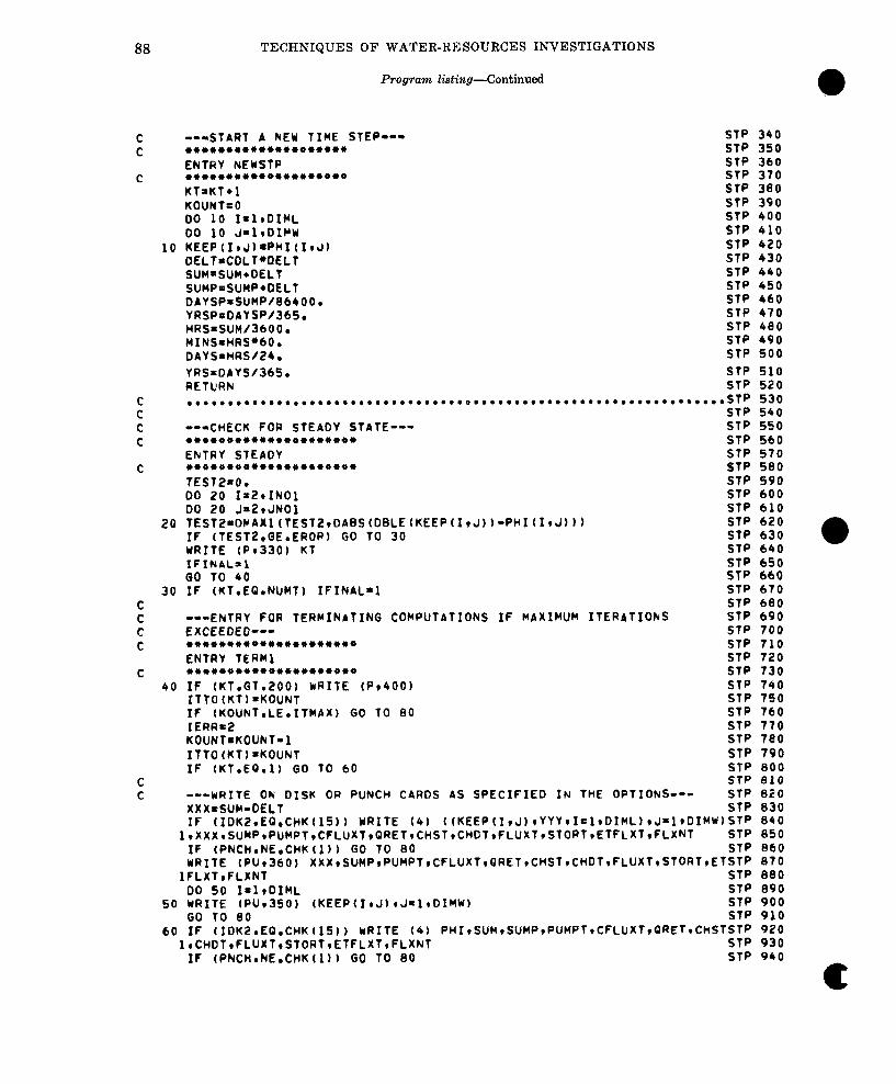
TECHNIQUES OF WATER-RESOURCES INVESTIGATIONS
Program listing--Continued
---START A NEW TIME STEP-- SIP 340 o**o+ao*o*o*ooOIoo*o STP 350 ENTRY NEYSTP SfP 360 l o*oo*oooo*444oo*o** STP 370 KT=KT*l STP 300 KOUNT=O STP 390 DO 10 I=lrOIHL SIP 400 00 10 J=lrOIMY STP 410 KEEP(IeJ)rPHI(IrJ) STP 420 OELT=CDLT*OELT STP 430 SUM=SUM+DELT STP 440 SUMP=SUMP*OELT STP 450 OAYSPISUMP/B~SOO. STP 460 YRSPoDAYSP/365r STP 470 HRS=SUM/3600. STP 480 MINS=HRS*60. STP 490 DAYS=HRS/24, STP 500
YRS=OAYS/365. STP 510 RETURN STP 520 . . . . . . . . . . . . . . . . . . . . . . . . . . . . . . . . ..~............................... stp 530
STP 540 STP 550 STP 560 STP 570 STP 580 STP 590 STP 600 STP 610 STP 620 STP 630 STP 640
0
---CHECK FOR STEADY STATE--- l o4o*4o4oo**o4o4oo*4o
ENTRY STEADY oo4o44ooo*o4*4*oo444o
TESTZ=O. 00 20 1=211NOl DO 20 J=ZvJNOl TEST2~DCAXl~TEST2~DABS~DBLE~KEEP~I~J~~~PHI~I~J~~~ IF (TEST2.GE.EROR) GO TO 30 WRITE (P1330) KT IFINAL= QO TO 40 IF (KT.EQ.NUWT) IFINAL=
---ENTRY FOR TERMINATING COMPUTATIONS If MAXIMUM ITERATIONS EXCEEDEO--- l **404*4440*444*04404
ENTRY TERM1 *4440*4*044*4*400****
If (KT.GT.200) MRITE (P*400) ITTO(KT)=KOUNT If (KOUNT.LE.ITMAX) GO TO 80 IEAR= KOUNTmKOUNT-1 ITT0 (KT) =KOUNT IF (KT.EQ.l) GO TO 60
---YRITE ON DISK OR PUNCH CARDS AS SPECIFIED IN THE OPTIONS---
STP 650 STP 660 STP 670 STP 600 STP 690 STP 700 STP 710 STP 720 SIP 730 STP 740 STP 750 STP 760 STP 770 STP 700 STP 790 STP BOO STP 010 STP 020 STP 830 XXX=SUM-DELI
IF (IDKZ.EQ.CHK(l5)) WRITE (4) ~~KEEP~I~J~rYYYtI=lrDIML~rJI1,DIMW~Sl~ 840 1rXXX~SUMP~PUMPT~CfLUXTIQRETICHSTICnDT~FLUXT~STORT~ETFLXT~fLXNT STP 850
IF (PNCH.NE.CHK(l)b GO TO 80 STP 060 WRITE (PUv360) XXXISUMPIPUMPT~CFLUXT,QRETICHST~C~DT,FLUXT~STORT~ETSTP 870
1FLXTeFLXNT STP 880 DO 50 I=ltDIML STP 890
50 WRITE (PU1350) (KEEP(ItJ)rJ=l,DIMb) STP 900 GO TO 00 STP 910
60 IF (IOK2.EQ,CHK(lS)) bRITE (4) PHIISUMISUMPIPUMPTICFLUXTIORETICHS~S~P 920 lrCHOTrFLUXTrSTORT,ETFLXTIFLXNT STP 930
If (PNCHmNE,CHK(l)) GO TO 80 STP 940
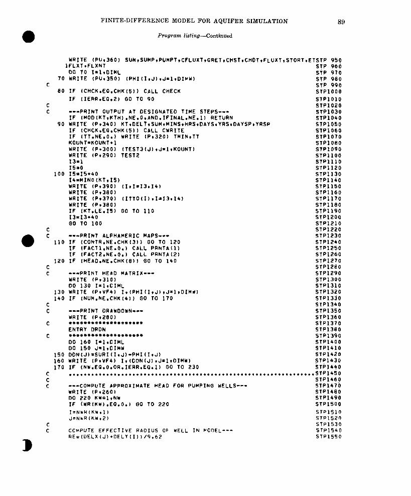
FINITE-DIFFERENCE MODEL FOR AQUIFER SIMULATION 89
Program listing-Continued
WRITE (PU1360) SUHISUHPIPUMPTICFLUXTIORETICHSTICHOTIFLUXT~STORT~E~STP 950 IFLXTrFLXNT STP 960
00 70 I=l,OIML sip 910 70 WRITE (PUe3SO) (PH1(11J)rJ=lr01~W) STP 980
C STi’ 990 80 IF (CHCK.EQ.CHK(5)) CALL CHECK STPlOOO
IF (IERR.EQ.2) GO TO 90 STPlOlO C STP1020 C ---PRINT OUTPUT AT DESIGNATED TIME STEPS--- STP1030
IF ~MOO(KT~KTH).NE.O.ANO.IFINAL.NE.l~ RETURN STP1040 90 WRITE (P1340) KT~OELTISUHIMINSIHRSIDAYS~YRS~DAYSP~YRSP STP1050
IF (CHCK.EQ.CHK (5) 1 CALL CWRITE STP1060 IF (TT.NE.0.) WRITE fP1320) TMI,NrTT STPlO70 KOUhT=KOUNT+l STP1080 WRITE (P*300) (TEST3tJ) tJ=lrKOUNT) STP1090 ;;I;’ (Pe290) TEST2 STPllOO
IS=0 S7PlllO STPll20
100 ISnI5*40 STPll30 II+HINO (KTeI5) STPllbO WRITE (Pw390) (It1=13r14) srq1150 WRITE (P1380) STPll60 WRITE (P1370) fITTO eI=13r14) STPll70 WRITE (P1380) stpiiao IF LKT.LE.15) GO TO 110 STPll90 x3=13+40 STPl200 GO TO 100 STPlElO
E STP1220
---PRINT ALPHAMERIC MAPS-r- STP1230 110 IF (CONTR.NE.CHK(J)) GO TO 120 STP1240
IF (FACTl.NE.0.) CALL PRNTA(1) STP1250 IF (FACT2.NE.0.) CALL PRNTA(2) STP1260
120 IF fHEAD.NE.CHK(G)) GO TO 140 STP1270 C S!P12EO C ---PRINT HEAD MATRIX--- STP1290
WRITE (P1310) STP1300 00 130 I’lrCIML STP1310
130 WRITE (PtVF4) II~PHI(I~J)~J=~~OIM~~ STP1320 140 IF (NUM.NE.CHKfQ)) GO TO 170 ST@1330
: STP1340
---PRINT DRAWOOWN~~- STP1350 WRITE fP9280) STP1360
C 0***00***0400**0*v** sip1370 ENTRY DRON STP1380
C l 0*00*00***00040000* STP1390 DO 160 I=lrOIML STP1400 00 150 J=ltCIMW STP1410
150 OON~J~~SURI(IIJ)-PHI~I~J) STPl420 160 WRITE (P*VF4) I~~DON(J)rJ=l,DIMW) STP1430 170 IF (NW.EO.O.OR.IERR.EQ.1) GO TO 230 kTb1430
C ,.............................,................,........~~*~a~~~~~ STP1450 C STP1460 C ---COMPUTE APPROXIMATE HEAD FOR PUMPING WELLS--- STP147b
WRITE (P12601 STP1480 DO 220 KY=l~NW STP1490 IF (WR~KW).EO.~.) GO TO 220 STPlSOO I=NWH(KW,l) STPlSlO J=NhR(KW*2) STP1520
c STP1530 C CChrPUTE EFFECTIVE RAOIIJS OF WELL IN MODEL--- SfP1540
STP1550
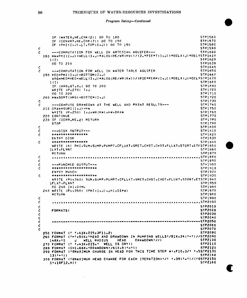
90 TECHNIQUES OF WATER-RESOURCES INVESTIGATIONS
Program listing--Continued
IF (WATER.NE.ChK(Z)) GO TO 180 STP1560 IF (CONVRT.NE.CHK(7)I GO TO 190 STPl570 IF ~PtlI~I,J).LT.TOP~I~J~l GO TO 190 STPl580
c STP1590 C ---COMPUTATION FOR WELL IN ARTESIAN AQUIFER--- STPl600
180 Hk=~HI~ItJ~*WELL~ItJ~Q6LOG~RE/WR~KW~~/~2.*PI~*T~I~J~~*DELX~J~*DELYSTPl6l~ l(I) STP1620
GO TO 210 STP1630 C STP1640 C ---COMPUTATION FOR WELL IN WATER TARLE AQUIFER STP1650
190 HED=PHI(I*J)-BOTTOM(I,J) STP1660 ARG=HED~HED~WELL~I~J~rALOG~RE/WR~Kw~~/~PIE*PER~~I~J~~*DELX~J~*DEL~ST~l670
l(I) STPl680 IF (ARG.GT.0.) GO TO 200 STP1690 WffITE (Pe270) I,J STP1700 GO TO 220 STP1710
200 HW=SQRT(ARGl*F!OTTOM(IvJl STP1720 C STP1730 C ---COMPUTE DRAWDOWN AT THE WELL AND PRINT RESULTS--- STP1740
210 DPAW=SURI(IVJ~-HW STP1750 WRITE IP1250) ItJI~R(K~)rH~aDRAtd STP1760
220 CONTINUE STP1770 230 IF (IERR.NE.2) RETURN STP17BO
STOP STP1790 C STP1800 C ---DISK OUTPUT--- STPlelO C, *********it****** STP1820
EhTRY DISK STPl830 C **************** STP1840
WRITE (4) PHIISUHISUMPIPUMPT,CFLUXT~QRET,CHSTICHDT*FLUXT*STDRT*~TFSTP~~~@ lLXT,FLXNT STP1860 0
RETURN STP1870 c . . . . . . . . . . . . . . . . . . . . . . . . . . . . . . . . . . . . ..*........................... STPl880 C STP1890 C ---PUNCHED OUTPUT--- STPl900 C ******************** STP1910
ENTRY PUNCh STPI920 C *o********o****o**** STP1930
WGITE (PU1360) SUH.SUMPIPUMPT~CFLUXTIOWETICHST,CHDT~FLUXT~STORT~ETSTP~~~O 1FLXTqFLXNT STP1950
DC 240 I=l,DIYL STPl960 240 WRITE (PU135o) (PHI(IIJ~*J=I~DIHW) STPl97n
RETURN STP1980 C STP1990 C . . . . . . . . . . . . . . . . . . . . . . . . . . . . . . . . . . . . . . . . . . . . . . . . . . . . . . . . . . . . . . . . . . STPZOOO
E STP2010
FORMATS I STP2020 C STPEOJO C STP2040 C ,-----------------------------------------------------------.-----~TP~Q~Q
STP2060 STP2070
250 FORMAT (’ ‘r43Xt215~3F11.2) STP2080 240 FORMAT (‘0’rSOXefHEAD AND DRAWDOWN IN PUMPlNG uELLS’/SlX.34(‘-‘,//~~~~~~~
148XI’I WELL RADIUS 270 FORMAT (’ t43X.215.’
HEAD DRAWDOWN’//) WELL IS DRY,) STPEllO
280 FORMAT ~lHlr6OXr’DRAWDOWN’/6lX~G~‘~‘~~ STP2120 290 FORMAT (,OMAXIMUM CHANGE IN HEAD FOR THIS TIME STEP =*rFlO.J/’ ‘r5STP2130
13(‘-0 1 STP2140 300 FORMAT ('OMAXIMUM HEAD CHANGE FOR EACH ITERATIONI’/@ @r39((-~)/(~OSTP2150
1~~10~12.4ll STP2160
c
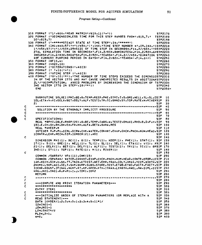
FINITE-DIFFERENCE MODEL FOR AQUIFER SIMULATION 91
C
C
Program Wing-Continued
310 FORMAT (‘1**60X**HEAO MAtRIX*/61X*ll(*-0) STP2170 320 FORMAT (‘ODIHENSIONLESS TIME FOR THIS STEP RANGES FROH**Gl5.7** TSTP2180
lO’tG15.71 STP2190 330 FORMAT (‘0**+4eSTEADY STATE AT TIME STEP**I4,“*4~4*1 STP2200 340 FORMAT ~lHl*44x*57~*-‘)/45X**~**l4X*‘TIME STEP NUMBER =‘r19,14XptlSTP2210
1*/45X*57(*-O//SOX*29HSIZE OF TIME STEP IN SECONDS=*Fl4.2//55X**TOSTP2220 2TAL SIMULATION TIME IN SECONDS=**F14.2/80X*8HMINUTESorF14.2/82X,6HSTP223O 3HOURS=*F14.2/83X*5HDAYS~*Fl4.2/82X**YEARS~**Fl4.2///45X**DURATION STP2240 40F CURRENT PUMPING PERIOD IN DAYS=*tF14.2/82X*‘YEARS=**Fl4.2//) STP2250
350 FORMAT (GF10.41 STP2260 360 FORMAT f4020.101 STP2270 370 FORMAT ~‘OITERATIONS1’*40I3l STP2280 380 FORMAT T’ ‘*lOf’-‘1) STP2290 390 FORMAT (‘OTIHE STEP I**40131 SfP2300 400 FORMAT (‘O**lO(***) ,‘THE NUMBER OF TIME STEPS EXCEEDS THE DIMENSIOSTP2310
1N OF THE VECTOR ITT0 AND MAY CAUSE UNEXPECTED RESULTS IN ADDITIONASTP2320 2L*/‘OCOCPUTATION. AVOID PROBLEMS BY INCREASING THE DIMENSION OF TSTP2330 3HE VECTOR ITT0 IN STEP’*lO(‘~*Ib STP2340
END STP2350-
SUGROUTINE SOLVEl~PHI*8E*G*TEMP*KEEP*PHE*STRT*T*S*QRE*WELL*TL*SL,DS lEL*ETA*V*XI*DELX*8ET*DELY*ALF*TEST3*TR*TC*GRND*SY*TOP*RATE*M*RIVERS 2) S
oooooooooooooooooooooooooooooooooooooooooooooooooooooooooo”ooooooo~ SOLUTION BY THE STRONGLY IMPLICIT PROCEDURE S
00000000000000000000000000000000000.0000000000000000000000000000~0~ S
SPECIFICATIONS: s REAL ~~PHI*DBLE,RHOP~20~*G*GE,TEWPtDABSIWlfES*W*TEST2*DMAXl*RHO*B,D*F*H*S
IGl*E*CH*GH*BH*Dti*EH*FHtHHtALFA*BETA*GAMA*RES S REAL l 4KEEP*M S INTEGER R*P*PU*DINL*DIMW*CHK*WATER*CONVRT*EVAP*CHCK*PNCH*NUM*HEADtS
lCONTR*LEAK*RECH*SIP*IORDER~2ll*ADI S S
DIMENSION PHI(l)* BE(l)* G(l)* TENP(l)* KEEP(l)* PHEtll* STRTfl)* S If(l)* S(l)* QRE(l)* WELL(l)* TLll)* SL(l)* DEL(l)* ETA(l)* v(l)* XS 2Ill)r DELX(l)* GET(l)* DELYtl) * ALF(l)* TEST3(1)* TR(l)* TC(ll* GRS 3ND(l)* SY(l)* TOP(l)* RATE(l)* H(l)* RIVER(l)
: COMMON /SARRAY/ VFQ(ll)*CHK(lS) S COMMON /SPARAM/ WATER*CONVRT*EVAP*CHCK*PNCH*NUH*HEAD*CONTR*EROR*LES
lAK*RECH*SIP*U*SS*TT*TMIN*ETDIST*QET*ERR*TMAX*CDLT*HHAX*YDIM,WIDTH*S 2NUMS*LSOR*AOI*DELTtSUM*SUMP*SUBS*STORE*TEST*ETGB*ETQD*FACTX*FACTY*S 3IERR~KOUNT~IFINAL~NUMT~KT~KPINPERIKTH~ITMAX~LENGTH~NWELtNW~DINL~DIS 4MW*JNOl*INOl*R*P*PU*I*J*IDKl*IDK2 S
RETURN S .*.............v.......*...,.,.................................... S
S ---COMPUTE AND PRINT ITERATION PARAMETERS--- *4*44444444444444444 z ENTRY ITERl S 444444444444444U4444 S ---INITIALIZE ORDER OF ITERATION PARAMETERS (OR REPLACE WITH A S READ STATEMENTl--- S DATA 10RDER/1*2v3*4*5*1*2*3*4*5*11~1/ S IZ=INOl-1 S JZ=JNOl-1 S LEaLENGTH/ S PLZ=LZ-1 l S
WPO. S
P 10 P 20 P 30 P 40 P 50 P 60 P 70 P eo P 90 P 100 P 110 P 120 P 130 P 140 P 150 P 160 P 170 P 180 P 190 P 200 P 210 P 220 P 230 P 240 P 250 P 260 P 270 P 280 P 290 P 300 P 310 P 320 P 330 P 340 P 350
,P 360 :p 370 :P 380 :P 390 iP 400
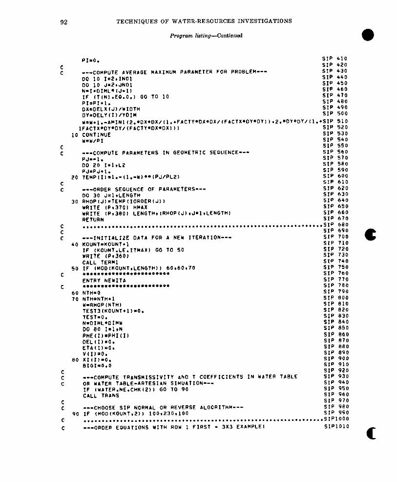
TECHNIQUES OF WATER-RESOURCES INVESTIGATIONS
Program l&ding-Continued
PISO. c
SIP 410 SIP 420
z ---COMPUTE AVERAGE MAXIMUM PARAMETER FOR PROBLEM--- SIP 430 DO 10 1=211NOl SIP 440 DO 10 J=2rJNOl SIP 450 N=I*OIML*tJ-1) SIP 460 IF (T(N).EQ.O.) GO 10 10 SIP 470 PI=PI+l. SIP 480 DX=OELX(J1/UIDTH SIP 490 DY=DELY(I1/YDIM SIP 500
u=w*1. ~AMINl(2.*DX~DX/(l.*FACTY*bXaOX/~FACTX~DY*DY~~~2.~DY*DY/~l.*SIP 510 1FACfX*OY*DY/(FACTY*DXoDXI)) SIP 520
CONTINUE SIP 530 Y8Y/Dl SIP 540
10
C C
. . mr. e
SIP 550
20 C C
30
---COMPUTE PARAMETERS IN GEOMETRIC SEQUENCE--- PJP-1. DO 20 I=lvL2 PJ=PJ*l. TEHP(I)rl.-(1.0W)**(PJ/PL2)
---ORDER SEQUENCE OF PARAMETERS---
C C C
40
DO 30 J=leLENGTH S RHOP(J)=TEMP(IORDER(J1) S WRITE 1P13701 HWAX S WRITE (Pv3801 LENGTHe(RHOP(J)rJ=lvLENGTH) S RETURN S . . . . . . . . . . . . . . . . . . . . . . . . . . . . . . . . . . . . . . . . . . . . . . . . . . . . . . . . . . . . . . . . . . S
S
50 C
C 60 70
---INITIALIZE DATA FOR A NEW ITERATION--- KOUNT=KOUNT*l IF (KOUNT.LE.ItMAX) GO TO 50 WRITE (Pt3601 CALL TERN1 IF (MOD(KOUNT,LENGTH) 1 60~6Oe70 ****00~**~**+00~~*~0*#v~ ENTRY NEWITP •~00~*~~~00*~,0***0~~~*~ NTH=O NTH=NTH+ 1 W=RHOP (NTH) TEST3(KOUNT*l)=O. TEST=O. N=D1ML*OIMW DO 80 I=l,N PHE(I)=PHI(Ib DEL(I)nOe ETr\(I)=O. V(I)rO. XI(Il~O. BIGI=O.O
P 560 P 570 P 580 P 590 P 600 P 610 P 620
‘P 630 P 640
‘P 650 :p 660 ‘P 670 :P 600 :P 690 :P 700 :P 710 :P 720 :fJ 730 :P 740 :P 750 :P 760
SIP 770 SIP 780 SIP 790 SIP 800 SIP 810 SIP 820 SIP 030 SIP 840 SIP a50 SIP 860 SIP 070 SIP 880
00
E C
C C
90 C
C
TABLE
SIP 890 SIP 900
---COMPUTE TRANSMISSIVITY AND T COEFFICIENTS IN WeTER OR WATER TABLE-ARTESIAN SIMUATION--- IF (WATER.NE.CHK(Z)) GO TO 90 CALL TRANS
SIP 910 SIP 920 SIP 930 SIP 940 SIP 950 SIP 960 SIP 970
---CHOOSE S1P NORMAL OR REVERSE ALGORITHM--- SIP se0 IF (MOO(KOUNT,Z)) lOOv230tlOO SIP 990 . . . . . . . . . . . . . . . . . . . . . . . . . . . . . . . . . . . . . . . . . . . . . . . . . . . . . . . . . . . . . . . . . . sIPlooo
---ORDER EQUATIONS WITH ROW 1 FIRST - 3X3 EXAMPLE! sIPlolo
c
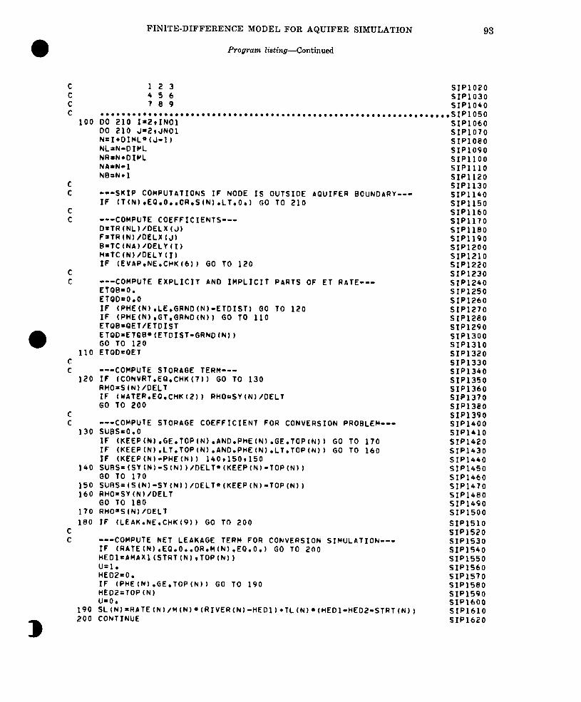
C C
C C
130
140
150 160
170 180
C C
190
B 200
FINITE-DIFFERENCE MODEL FOR AQUIFER SIMULATION
Program listing--Continued
93
12 3 SIP1020 456 SIP1030 789 SIP1040
. . . . . . . . . . ..~.....................................................sIPloso DO 210 1=211NOl SIP1060
SIP1070 DO 210 J=ZtJNOl N=I*OIML*(J-1) NL-N-DIKL NR=N*OIKL N&=N-1 NB=N+ 1
---SKIP COMPUTATIONS IF NODE IS OUTSIDE AQUIFER BOUNDARY--- IF ~f(N~.EQ.O..OR,S~N~.Ll.O.~ GO TO 210
---COMPUTE COEFFICIENTS--- D=lR(NL)/DELX(J) F*TR(N)/DELX(J) B=TCfNA)/DELY(I) H=TCtN)/DELY (1) IF (EVAPeNE.CHK(6)) GO TO 120
---COMPUTE EXPLICIT AND IMPLICIT PARTS OF ET RATE--- ETQB=O. ETQDaO.0 IF (PHE~N).LE.GRNO(N)~ElDISl) GO TO 120 IF (PHE(N)rGf.GRkD(N)) GO TO 110 ETQB=QET/ETOIST ETQD=ETQB’(ETDIST-GRND IN) ) GO TO 120 ETQD=QET
---COMPUTE STORAGE TERM--- IF (CONVRT.EQ.CHK(7)) GO TO 130 RHO’S(N) /DEL1 IF (WATER.EQ.CHK(2)) RHO~SY(N)/DELT GO TO 200
---COMPUTE STORAGE COEFFICIENT FOR CONVERSION PRDBLEW--- SUBS=O.O IF (KEEP~N~.GE.TOP(N).AND.PHE~N).GE.TOPo) GO TO 170 IF (KEEP(N).LT.TOP(N).ANO.PHEfN).LT.TOP(N)) GO TO 160 IF (KEEP(N)-PHEtN) 1 140tlSOr150 SUBS=(SY(N)-S(N))/DELT”(KEEPtNj-TOP(N)) GO TO 170 SUBS=(S(N)-SY(N))/DELTO(KEEP(N)-TOP(N)) RHO=SY (N) /OELT GO TO 180 RHO’S(N) /DELT IF (LEAK.NE.CHK(9)) GO TO 200
---COMPUTE NET LEAKAGE TERM FOR CONVERSION SIMULATION--- IF (RATE(N).EQ.O..OR.H(N).EQ.O.) GO TO 200 HEOl=AHAXA (STRT (N) tTOP (N) 1 U=l. HEDZ=O. IF (PHEtN) .GE.TOP(N)) GO TO 190 HEOZ-TOP (N) u=o. SL(N~=RATE(N)/M(N)*(RIVER(N)-HEDl)~TL(N)~(HEDl-HED2.STRT(N)) CONTINUE
SIPlO@ SIP1090 sIPlloo SIP1110 SIP1 120 SIP1 130 SIP1 140 SIP1 150 SIP1160 SIP1170 SIP1180 SIP1190 SIP1200 SIP1210 SIP1220 SIP1230 SIP1240 SIP1250 SIP1260 SIP1270 SIPlzeo SIP1290 SIP1300 SIP1310 SIP1320 SIP1330 SIP1340 SIP1350 SIP1360 SIP1370 SIP13BO SIP1390 SIP1400 SIP1410 SIP1420 SIP1430 SIP1440 SIP1450 SIP1460 SIP1470 SIP1480 SIP1490 SIP1500 SIP1510 SIP1520 SIP1530 SIP1540 SIP1550 SIP1560 SIP1570 SIP1580 SIP1590 SIP1600 SIP1610 SIP1620
94 TECHNIQUES OF WATER-RESOURCES INVESTIGATIONS
Program listing--Continued
C S IP1630 C ---SIP (NORMAL’ ALGORITHM--- S IP1640 C ---FORWARD SUBSTITUTE, COMPUTING INTERMEDIATE VECTOR V-.,-
E=-B-01F-H-RHO-TL(N)*U-ETQG s’ It’1650 IP1660
CH=OEL(NA~“B/(l.+W~DEL(NA)) S IP1670 GH=ETA(NLb*O/(l.+w*ETA(NL)I S IPl6GO BH=B-W*CH S IP1690 DH=D-w*GR SIPlfOO EHoE+W*CH*W*GH SIP1710 FH=F-W*CH SIP1720 HHoH-W”GH SIP1730 ALFA=BH SIP1740 BETA=DH SIP1750 GAHA=EH-ALFA*ETAtNA)-BETA*DELtNL) SIP1760 DEL(N)=FH/GAMA SIP1770 ETA(N)PHH/GAHA SIP1780 RES=-D*PHI~NL~~F*PHI~NR~~H~PHI~NB~~B~PHI(NA~~E*PHI~N~~RHO*KEEP~N~~SIPl79O
lSL(N)-ORE(N)-WELL(Nb+ETQD-SUES-TLo,STRTtNb sIPleo V(N)=(HNAX*RES-ALFA*V(NA)-BETA*VtNLlb/GAMA SIPlf310
210 CONTINUE SIP1620
E SIP1830
---BACK SUBSTITUTE FOR VECTOR XI--- SIP1840 DO 220 I=lrI2 SIP1850 13=DIML-I SIP1860 DO 220 J=lrJZ SIP1870 J3=OIMw-J SIP1880 N=I3+DINL*(J3-11 SIP1890 IF (TtN)aEQ.O..OR.S(N).LT.O.) GO TO 220 S1P1900 XIIN)=VtN)-OEL(N)*XI(N+OIML)-ETP(N)rXI(N+il SIP1910
C SIP1920 C ---COMPARE MAGNITUDE OF CHANGE WITH CLOSURE CRITERION-- SIP1930
TCHK=ABS (XI (N) 1 SIP1940 IF (TCHKeGT.BIGI) BIGI=TCHK SIP1950 PHI(N)rPHI(N)+XI(NI SIP1960
220 CONTINUE SIP1970 IF tBIGI.GT.ERR) TEST=l. SIP1980 TEST3(KOUNT+l)=BIGI SIP1990 IF (TEST.EQ.l.) GO TO 40 SIP2000
RETURN SIP2010 C SIP2020 C . . . . . . . . . . . . . . . . . . . . . . . . . . . . . . . ..~................................SIP2030 C ---ORDER EQUATIONS WITH THE LAST ROW FIRST - 3X3 EXAMPLE1 SIP2040 C 7 8 9 SIP2050
E 456 SIP2060 12 3 SIP2070
C . . . . . . . . . . . . . . . . . . . . . . . . . . . . . . . ..~................................ SIP2000 230 DO 340 11=1*X2 SIP2090
I=DIML-II SIP2100 DO 340 J=2rJNOl SlP2110 N=I*DIHL*(J-lb SIP2120 NL=N-DIML SIP2130 NR=N*DINL SIP2140 NAoN-1 SIP2150 NB=N*l SIP2160
C SIP2170 C ---SKIP COMPUTATIONS IF NODE IS OUTSIOE AQUIFER BOUNDARV--- SIP2180
IF (TfN)eEQ.O..OR.S(N).LT.O.b GO TO 340 SIP2190 C SIP2200 C ---COMPUTE COEFFICIENTS--- SIP2210
D=TR(NL)/OELXtJb SIP2220 F=TR(N)/DELX(J) SIP2230
C C
240 C C
250
C C
260
270
280
0 290
300 310
E
320 330
C
FINITE-DIFFERENCE MODEL FOR AQUIFER SIMULATION
Program listing--Continued
B=TCfNA)/DELY(Ib H=TC(N)/DELYfI) IF (EVAP.NE.CHK(6)) GO TO 250
---COMPUTE EXPLICIT AND IMPLICIT PARTS OF ET RATE--- ETQG=O, ETQO=O.O IF (PHE(N).LE.GRNOfN)-ETOIST) GO TO 250 IF (PHE(N) .GT.GRNOfN) 1 GO TO 240 ETQE=QET/ETOIST ETQO=ETQB*~ETOIST-GRNO (N) 1 GO TO 250 ETQO=QET
---COMPUTE STORAGE TERM--- IF (CONVRT.EQ.CHKfI)) GO TO 260 RHO=S(N)/OELT IF (YATER.EQ.CHK(Z)) RHO=SY(N)/OELT GO TO 330
--COMPUTE STORAGE COEFFICIENT FOR CONVERSION PRO5LEb-- SUBS=O.O IF (KEEP(N) *GEeTOP (N) .ANOIPHE(N) .GE.TOP(N) 1 Go TO 300 IF (KEEP(N) .LT,TOP(N) .ANO.PHE(Nb .LT.TOP(N) 1 GO TO 290 IF (KEEP(N)-PHE(N)) 270r280t280 SUGS=(SY(N)-S(N))/OELf*(KEEP(N)-TOP(N)) GO TO 300 SUBSa(S(N)-SY(N))/DELT*(KEEP(N)) RHO=SY (N) /OELT GO TO 310 RHO=S (Nb /DEL1 IF (LEAK.NE,CHK(P)) GO TO 330
---COMPUTE NET LEAKAGE TERM FOR CONVERSION SIMULATION--- IF (RATE~N).EQ.O..OR.K(N~.EQ.O.~ GO TO 330 HEOl=AMAXl(STRT~N)rTOP(N)) Wl. HEOZ=O. IF tPHE(N) .GE.TOP(N) 1 GO TO 320 HEOZ=TOP (N) u=o. SL~N~=RATE(N)/M~N)*~RIVER~N)-HEOl~~TL(N)~~HEDl~HEO2~STRT(N~~ CONTINUE
---SIP *REVERSE@ ALGORITHM--- ---FORWPRO SUBSTITUTEI COMPUTING INTERMEDIATE VECTOR V--- E=-B-O-F-n-RHO-TL(N).U-ETQG CH=OEL(NB)*H/flo~W*OEL(NG)~ GH=ETA~NL)*O/(l~*W*EfA(NL)) GH=H-W*CH OH=O-W*GH EH=E+W*CH*W*GH FH=F-W*CCI HH=0-W*GH ALFA=GH GETA=On GAHA=EH-ALFA*ETA(NG)-GETAOOELtNL) OELfN)=FH/GAMA ETA (N) =HW/GAMA
95
SIP2240 SIP2250 SIP2260 SIP2270 SIP2280 SIP2290 SIP2300 SIP2310 SIP2320 SIP2330 SIP2340 SIP2350 SIP2360 SIP2370 SIP2380 SIP2390 SIP2400 SIP2410 SIP2420 SIP2430 SIP2440 SIP2450 SIP2460 SIP2470 SIP2480 SIP2490 SIP2500 SIP2510 SIP2520 SIP2530 SIP2540 SIP2550 SIP2560 SIP2570 SIP2580 SIP2590 SIP2600 SIP2610 SIP2620 SIP2630 SIP2640 SIP2650 SIP2660 SIP2670 SIP2680 SIP2690 SIP2700 SIP2710 SIP2720 SIP2730 SIR2740 SIP2750 SIP2760 SIP2770 SIR2780 SIP2790 sIR2Goo SIP2810 SIR2820
96 TECHNIQUES OF WATER-RESOURCES INVESTIGATIONS
Program listing-Continued
V(N)=(HHAX*RES-ALFA*V(Ne~-BETA*V(NL))/GAMA SIP2050 340 CONTINUE SIP2860
C SIP2870 C ---BACK SUBSTITUTE FOR VECTOR XI--- SIP28@0
DO 350 13=2,INOl SIP2R90 DO 350 J-lrJ2 SIP2900 JhDIMW-J SIP2910 N=IJ+DINL”(J3-1) SIP2920 IF (T(N1.EP.O..OR.S(N).LT.O.1 GO TO 350 SIP2930 XI(N1=V(N1-OEL(N)*XI~N*OIML1-ETA~Nl”X1~N~l~ SIP2940
C SIP2950 C ---COMPARE MAGNITUDE OF CHANGE WITH CLOSURE CRITERION- SIP2960
TCHK=ABS (XI (N) 1 SIP2970 IF ITCHK.GT.BIGI) BIGI=TCHK SIP2980 PHI (N)=PHI (N)*XI (N1 SIP2990
350 CONTINUE SIP3000 IF tBIGI.GT.ERA) TEST=l. SIP3010 TEST3(KOUNT*l)=BIGI SIP3020 IF (TEST.EQ.l.1 GO TO 40 SIP3030 RETURN SIP3040
C SIP3050 C . . . . . . . . . . . . . . . . . . . . . . . . . . . . . . . . . . . . . . . . . . . . . . . . . . . . . . . . . . . . . . . . . . SIP3060 C SIP3070 C ---FORMATS--- SIP3080 C SIP3090 C ,,,,,,,,-,,,,,,,-----,---------------------------------------------SIp3100 C C
360 FORMAT (‘OEXCEEDEO PERMITTED 370 FORMAT (*-qr44Xv@SOLUTION BY
143(‘,‘),//,61X*‘BETA=‘*F5.2~ 380 FORMAT (lHO115.22ti ITERATION
END
SIP31 10 SIP3120
NUMBER OF ITERATIONS*/’ *t39(‘*0) SIP3130 THE STRONGLY IMPLICIT PROCEDURE’/~~XISIP~~~O 0
SIP3150 PARAMETERS:r6015.7/~/28XIbD15,7/)) SIP3160
SIP3170-
SUBROUTINE SOLVE2(PHI~BE,G,TEMP~KE~P~PHEISTRTITISIQRE,WELL~TL~SL,CSOR 10 ~ELIETAIVIXI~DELXIBETAIDELYIALFAITEST~~TR,TC~QRND~SY~TOP~RAT~~M~RIVSOR 20 2ER) SOR 30
------------------------------------------------------------------SOR 49 SOLUTION BY LINE SUCCESSIVE OVERRELAXATION SOR 50 ------------------------------------------------------------------SOR 60
SOR 70 SPECIFICATIONSr SOR 00 REAL *BPHI~DBLE~RH0P~20~rGIBEITEMPIIHKIDABS~W~PARAM~TEST2~D~AXl~P2SOR 90
I,AICIB~~EIQ~RHO~B~DIFIH SOR 100 REAL “4KEEPgM SOR 110 INTEGER R~P~PU~DINL~DIMW~CHKIW~TERICONVRTIEVAPICHCK,PNCH~NUM~HEAD~SOR 120
~CONTR~LEAKIRECHISIP~AOI SOR 130 SOR 140
DIMENSION PHIll)r BE(l)* G(l)* TEMP(l)v KEEP(l)* PHE(11, STRT(l)r SOR 150 1Ttl)r S(l)* QREtl)r WELL(l)* TL(l)r SL(l), DEL(l)* ETA(l)* v(l)* XSOR 160 21(l)* DELX(ljr BETA(l)* DELY(l)r ALFA( TEST3(lbr TR(l)r TC(I). SOR 170 3GRNOfl)r SY(l)r TOP(l)+ RATE(l)+ Htl)r RIVER(l) SOR 160
SOR 190 COMMON /SARRAY/ VF4(111rCHK(lS) SOR 200 COMMON /SPARAM/ ~ATERICONVRT,EVAPICHCKIPNCHINUM,HEAD,CONTR~EROR~LESOR 210
~AK,RECH~SIPIU~SSITTITMIN,ETDISTIQETIEAR~TMAX~CDLT~HMAX~YDIM,WIDTH~SOR 220 2NUMS~LSOR~ADItDELTrSUM~SUMP~SURStSTOREtTEST~ETQB~ETQD~FACTX,FACTY~SOR 230 ~IERR~KOUNT~IFINAL~NUMTIKTIKPINPERIKT~~ITMAX~LENGTH~NWEL~NW~DIML~DISOR 240 4HKrJNOlrINOlrR~P~PUtlrJtIDKlrIDK2 SOR 250
RETURN SOR 260
FINITE-DIFFERENCE MODEL FOR AQUIFER SIMULATION
Program listing--Continued
97
C . . . . . . . . . . . . . . . . . . . . . . . . . . . . . . . . . . . . . . . . . . . . . . . . . . . . . . . . . . . . . . . . . . SOR 270 c SOR 280 C ---WRITE ACCELERATION PARAMETER--- SOR 290 C 0o00ooooooooooo0ooooo SOR 300
ENTRY ITERZ SOR 310 C oOooOoooooooooo*oooOo SOR 320
YRITE (Pe490) SOR 330 WRITE (PvsOO) HMAXII.ENOTH SOR 340 RETURN SOR 350
C . . . . . . . . . . . . . . . . . . . . . . . . . . . . . . . . . . . . . . . . . . . . . . . . . . . . . . . . . . . . . . . . . . SOR 360 C SOR 370 c ---INITIALIZE DATA FOR A NEW ITERATION--- SOR 300
10 KOUNT=KOUNT+l SOR 390 IF (KOUNT.LE.ITMAX) GO TO 20 SOR 400 IJRITE (Peslo) SOR 410 CALL TEAM1 SOR 420
C ~O~OOOOOO*~OOOOO~OO~OOOO SOR 430 ENTRY NEWITB SOR 440
C oooo0o0oo0*0oo0ooOOooooo SOR 450 20 TEST3(KOUNT*l)=O. SOR 460
TEST=O. SOR 470 NoDIML*DI~W SOR 480 DO 30 I*lpN SOR 490
30 PHE(I)=PHI(I) SOR 500 BIGImO.0 SOR 510
C SOR 520 C ---COMPUTE TRPNSNISSIVITY AND 1 COEFFICIENTS IN WATER TABLE SOR 530 C OR WATER TAeLE-ARTESIAN SIMUATION--- SOR 540
IF (WATER.NE.CHK(E) 1 GO TO 40 SOR 550 CALL TRANS SOR 560
C . . . . . . . . . . . . . . . . . . . . . . . . . . . . . . . . . . . . . . . . . . . . . . . . . . . . . . . . . . . . . . . . . . SOR 570 C SOR 580 C ---SOLUTION BY LSOR--- SOR 590 C ---------------------- SOR 600
40 NO3oOIMlr-2 SOR 610 TEMP (DIMU)=O.O SOR 620 DO 170 1=2rINOl SOR 630 00 150 ‘J’2rJNOl SOR 640 N=I’DIML*(J-1) SOR 650 NA=N- 1 SOR 660 NB=N* 1 SOR 670 NL=N-OIHL SOR 680 NR=N+DIHL SOR 690 GEfJ)=O.O SOR 700 GtJ)=O,O SOR 710
c SOR 720 C ---SKIP COMPUTATIONS IF NODE IS OUTSIDE AQUIFER BOUNDARY--- SOR 730
IF (T(N).EQ.O..OR.S(N).LT.O.) GO TO 150 SOR 740 c SOR 750 C ---COMPUTE COEFFICIENTS---
D=TR(N-OIML)/DELX(J) F=TR(N)/DELXfJ) G=TCfN-l)/OELYfI) H=TC(N)/DELY (II IF (EVAP.NE.CHK(6) 1 GO TO 60
C C ---COMPUTE EXPLICIT AND IMPLICIT PARTS OF ET RATE---
ETQG=O. ETQD=O. 0 IF (PHE(N).LE.GRNO(N)-ETDISf) GO TO 60 IF (PHE(N).GT.GRND(N)) GO TO 50
SOR 760 SOR 770 SOR 780 SOR 790 SOW 800 SOR 810 SOR 820 SoR 030 SOR 840 SOR 850 SOR 860 SOR 070
98 TECHNIQUES OF WATER-RESOURCES INVESTIGATIONS
50 C C
60
C C
70
80
90 100
110 129
C C
130 140
C C
150
c”
160 C C
C C
170
Program listing--Continued
ETQB=QET/ETDIST ETQD=ETO8”(ETDIST-ORNO( GO TO 60 ETOD=QET
---COMPUTE STORAGE TERM--- IF fCONVRT.EQ.CHKfI)) GO TO 70 RHO=S fN) /DELI IF (WATEA.EQ.CHK (2) b RHO-SY (N) /DELT GO TO 140
---COMPUTE STORAGE COEFFICIENT FOR CONVERSION PROBLEM--- SUES=O.O IF (KEEPfN).GE.TOPfN~.AND.PHE~N).GE.TOPo) GO TO 110 IF (KEEP(N).LT.TOP~N).AND.PHE~N~.Ll.TOPO) GO TO 100 IF (KEEP(N)-PHEtN) 1 80,9Ov90 SUBS=(SY (Fo-S(N) )/DELT*fKEEP(N)-TOP(N)) GO TO 110 SUBS=(SfN)-SY(N))/DELTO(KEEP(Nk-TOP(N)) ~~0;~‘~~~‘““’
RHO=S (N) /DELT IF (LEAK.NE.CHK(P)b GO TO 140
---COMPUTE NET LEAKAGE TERM FOR CONVERSION SIHULATION--- IF (RAtE(N~.EQ.O..OR.M(N).EQ.O.~ GO TO 140 HEDl=AMAXl(STRT(N)rTOP(N)) U=l* HEOZ=O. IF tPHE(N).GE.TOP(N)) GO TO 130 HED2=TOP (N 1 U-0.
--FORWARD SUBSTITUTE9 COMPUTING INTERMEDIATE VECTOR G-m- Em-D-F-B-HoRHO-TL(N)*UIETQB W-E-D*GE(J-1) BE(J)=F/h
SOR 880 SOR 890 SOR 900 SOR 910 SOR 920 SOR 930 SOR 940 SOR 950 SOR 960 SOR 970 SOR 980 SOR 990 SORlOOO SORlOlO SOR1020 SOR1030 SOR1040 SOR1050 SOR1060 SORlO70 SOR1080 SOR1090 S0~1100 SORlllO SORll20 SORl130 sORll40 SOR1150 SORll60 SOR1170 S0R1180 SOR1190 SoRl200 SORl210 SOR1220 SOR1230 SOR1240 SOR1250 SOR1260
G(J)*tQ-D*G(J-1)1/W CONTINUE
---BACK SUBSTITUTE FOR TEMP.-- DO 160 KN04rlqN03 NOQ=DIMY-KN04 TEMP~N04)=G(N04)-8E(NO4~*TEMP~NO4+1) CONTINUE
---EXTRAPOLATED VALUE OF PHI--- 00 170 J=2tJNOl N=I+DIML*(J-11 PHI~N)=PHI(N)+HMAX~TEMP~J)
---COMPARE DIFFERENCE WITH CLOSURE CRITERION- TCHK=DABS(TEHPtJ)) IF (TCHK.GT.BIGI) BIGI=TCHK CONTINUE IF tBIGI.GT.ERR) TEST=l. TEST3(KOUNT+l)=BIG!
SOR1290 SOR1300 SOR1310 SOR1320 SOR1330 SOR1340 SORl350 SOR1360 SOR1370 SOR1380 SOR1390 SOR1400 SOR1410 SOR1420 SOR1430 SOR1440 SOR1450 SOR1460 SOR1470 SOR14BO
FINITE-DIFFERENCE MODEL FOR AQUIFER SIMULATION 99
C C
180
190
C C C C C C
200
210
C C
C C
220 C C
230
Program listing--Continued
IF (KOUNT.EQ.0) GO TO 10 SOR1490 IF fTEST.EQ.0.) RETURN SOR1500
SOR1510 ---TEST FOR TWO DIMENSIONAL CORRECTION--- SOR1520 IF (MOO~KOUNTtLENGTH).NE.O) GO TO 10 SOR1530 GO TO 200 SOR1540 DO 190 1=2tINOl SOR1550 DO 190 J=2tJNOl SOR1560 N=I+DIML+ (J-1) SOR1570 IF (T(Nl.EQ.0.) GO TO 190 SoRlSBO PHI(N)=PHI(N)*ALFA(I)+BETAtJ~ SOR1590 CONTINUE SOR1600 GO TO 10 S0R1610 . . . . . . . . . . . . . . . . . . . . . . . . . . . . . . . . . . . . . . . . . . . . . . . . . . . . . . . . . . . . . . . . . . SORl620
SOR1630 ---TWO DIMENSIONAL CORRECTION TO LSOR--- SOR1640 -------------------------I---------------- SOR1650
SOR1660 CORRECTION FOR ROWS--- SOR1670
SOR1680 SOR1690 SOR1700 SORl710 SOR1720 SOR1730 SOR1740 SOR1750 SOR1760 SOR1770
---COMPUTE ALFA DO 210 I’lrDIML ALFA(I)=O. BE(I)=O.O G(I)=O.O DO 330 I=Z~INOl A=O, B2=0. C=O. Q=O.
--SUMMATION OF DO 320 J=ZtJNOl N=I+DIML’(J-1) NA=N-1 NB=N+ 1 NL=N-DIML NR=N*DIHL IF (S(N) l LT.0.) IF (T(N) l EQ.0.)
COEFFICIENTS FOR EACH ROW---
GO TO 330 GO TO 320
---COMPUTE COEFFICIENTS--- DoTR(N-DIRL)/DELX(Jl F=TR(N)/DELX(J) B=TC(N-l)/DELY(I) H=TC(N)/DELY (11 IF (EVAP.NE.CHK(6)) GO TO 230
---COMPUTE EXPLICIT AND IMPLICIT PARTS OF ET RATE--- ETQB=O. ETQD=O.O IF (PHE(N).LE.QRND(N)-ETDIST) GO TO 230 IF (PHEtN) .GT.GRND(N) 1 00 TO 220 ETQB=QET/ETDIST ETQD=ETQE@(ETDIST-GRNDtN)) GO TO 230 ETQD=QET
---COMPUTE STORAGE TERM--- IF (CONVRT.EQ.CHK(7)) GO TO 240 RHO=S (N) /DELT IF (WATER.EQ.CHK(Z)) RHO=SY(N)/DELT GO TO 310
SOR17BO SOR1790 SORlGOO SORlGlO Son1620 SORlG30 SORlG40 SOR1850 SOR1860 SORlG70 SORlG@O SORlG90 SOR1900 SOR1910 SOR1920 SOR1930 SOR1940 SOR1950 SOR1960 SoR1970 SOR1980 SOR1990 SOR2000 SOR2010 SOR2020 SOR2030 SOR2040 SOR2050 SOR2060 SOR2070 SORE000 SOR2090
300 TECHNIQUES OF WATER-RESOURCES INVESTIGATIONS
240
250
260 270
200 290
C C
300 310
C
Program listing-Continued
SU0S~O.O IF (KEEP (N) .QE.TOP (N) .AND.PHE (N) .GE.tOP (N) 1 00 TO 280 IF (KEEP(N) .Ll.TOP(N) .AND.PHE(N) .LT.TOP(N) 1 00 TO 270 IF (KEEP(N)-PHEiN) I 250,260t260 SUBS=(SY (N)-S(N) )/DELT*(KEEP(N)-TOP(N)) GO TO 280 SuBS=(S(Nl~SY(Nl~/OELT=~KEEP~N)~TOP(N~) RHO=SY (N)/OELT (30 TO 290 RHO=S(N)/DELT IF (LEAK.NE.CHK(9)) 00 TO 310
---COMPUTE NET LEAKAGE TERM FOR CONVERSION SIMULATION--- IF (RATE(N) .EQ.O..OR.M(N) ,EQ.O.) GO TO 310 HEDl=ANAXl(STRT(N~,TOP(N)~ Ml. HEDE=O. IF (PHE(N).OE.TOP(N)) 00 TO 300 HEDZ=TOP (N) U=O. SL(N)=RATE(N)/M(N)=(RIVER(N)-HEDl)~TL(N)*(HEDl-HED2-STRT(N)) CONTINUE
AsA- Bl=B+H+RHO~TL(N)*U*ETQB 82=BZ+B 1 C=C-H
SOR2100 SoR2110 SoR2120 SOR2130 SOR2140 SOR2150 SOR2160 SOR2170 SOR21-90 SOR2190 SOR2200 SOR2210 SOR2220 SOR2230 SoR2240 SOR2250 SOR2260 SOR2270 SOR2200 SOR2290 SOR2300 SOR2310 SOR2320 SOR2330 SOR234 0 SOR235 0 SOR2360
Q=Q~(D~PH~(NL)~F=PHI~NR~*~=PHI~NA~~H=PHI~N~~~RHO=KEEP~N~~SL~N~+QRESOR237~ 1(N)+uELL(N)-ETQD~SU~S~TL(N)*STRT(N)-~D~F+Bl)=PHI~N)) SOR2380
320 CONTINUE SOR2390 C SOR2400 C ---COMPUTATION OF INTERMEDIATE VECTOR G--- SOR2410
W=82-AWE (I-1) SOR2420 BE(I)=C/= SOR2430 G(I)=(Q-A=O(I-l))/Y SOR2440
330 CONTINUE SOR2450 C SOR2460 C --BACK SUBSTITUTE FOR ALFAg-- SOR2470
N03=DIML-2 SOR2460 DO 340 KN04=1,N03 SOR2490 NOQ=DIML-KNO4 SOR2500
340 ALFA(N04)=G(N04)-8E(NO4)=ALFA(NO4+1) SOR2510 C eeeeeeeeeeeeeeeeeeeeeeeeeeeeeeeeeeeeeeee~eeeeeeeeeeeeeeeeeeeeeeeeesoR2520
E SOR2530
---COMPUTE BETA CORRECTION FOR COLUMNS--- SOR2540 DO 350 J=lrDIHW SOR2550 BETA (J)=O. SOR2560 BE(Jl=O.O SOR257 0
350 G(J)=O.O SOR2560 DO 470 J=2rJNOl SOR2590 A=09 SOR2600 82=0, SOR2610 c=o* SOR2620 Q=O. SOR2630
C SOR2640 C ---SUMMATION OF COEFFICIENTS FOR EACH COLUMN--- SOR2650
DO 460 1=29INOl SOR2660 N=I+DIML*(J-1) SOR2670 NA=N-1 SOR2600 NB=N+l SOR2690 NL=N-DIML SOR2700
FINITE-DIFFERENCE MODEL FOR AQUIFER SIMULATION
Program listing--Continued
NR=N*DIML IF (S(N1.LT.O.) GO TO 470 IF (T(N1.EQ.O.) GO TO 460 D=TA(N-DIML)/DELX(Jb F=tR(N)/DELX(J) 88TC(N-l)/OELY(I) H=TC(N)/DELY (I) IF (EVAP.NE.CHK(6)) GO TO 370
C C ---COMPUTE EXPLICIT AND IMPLICIT PARTS OF ET RATE---
ETQB-0. ElQD=O.O IF (PHE(F0 .LE.GRND(N)-ETDIST) GO TO 370 IF (PHE(N).GT.GRND(N)) GO TO 360 ETQB=QET/ETDIST ETQD=ETQB*(ETDIST-GRND(Nb) GO TO 370
360 ETQDsQET
---COMPUTE STORAGE TERM--- 370 IF (CONVRT.EQ.CHK(I) 1 GO TO 380
RHD*S(N)/DELT IF (WATER.EQ.CHK(Z)) RHO=SY(N)/DELT GO TO 450
C C ---COMPUTE STORAGE COEFFICIENT FOR CONVERSION PROGLEM---
3eo sues=o.o IF (KEEP(N) .GE.TOP (N) .AND.PHE (N) .GE.TOP(N) ) GO TO 420 IF (KEEP(N) .LT.TOP(N) .AND.PHE(N) .LT.TOP(N) 1 GO TO 410 IF (KEEP (N)-PHE (N) 7 3901400r400
390 SUGS=(SY(N)-S(Nb)/DELT*(KEEP(N)-TOP(N)) GO TO 420
400 SUBS=(S(N)-SY(N))/DELT”(KEEP(N)-TOP(N)) 410 RHO=SY (N)/DELT
GO TO 430 420 RHO=S(N)/DELT 430 IF (LEAK.NE.CHK(9)) GO TO 450
C C ---COMPUTE NET LEAKAGE TERM FOR CONVERSION SIMULAlION---
IF (RATE(N~,EQ.O..DR.W(N).EQ.O.~ GO TO 450 HEDl=AMAXl(STRT(N)~TOP(N)) Wl. HEDE=O, IF (PHE(N) .,GE.TOP(N) 7 GO TO 440 HEDt=TOP (N) wo.
440 SL~N~=R~TE~N~/W~N)*~RIV~R~N~IHED1)*TL~N~~(HEDl-HED2-STRT~N~~ 450 CONTINUE
C AI/L-D Gl=D*F*RHO*TL(N)*U*ETQl3 82=82+Ell CM-F
SOR2710 SOR2720 SOR2730 SOR2740 SOR27SO SOR2760 SOR2770 SOR2760 SOR2790 SoR2800 SOR2810 SOR2820 SOR2830 SOR2840 SOR2850 SOR2860 SOR2870 SOR28GO SOR2890 SOR2900 SOR2910 SOR292 0 SOR2930 SOR2940 SOR2950 SORE960 SOR2970 SOR2900 SOR2990 SoR3000 SOR3010 SOR3020 SOR3030 SOR3040 SOR3050 SOR3060 SOR3070 SOR3080 SOR3090 SOR3100 SOR3110 SOR3120 SOR3130 SOR3140 SOR3150 SOR3160 SOR3170 SOR3180 SOR3190 SOR3200 SOR3210 SOR3220 SOR3230
QIQ~(D*PHI(NL)+F~PHI(NR~+G~PHI(NA)+H~PHI(NG~~RH~*KEEP(N)~SL(N~*QRES~R~~~O l(N)~wELL(N)~~ETQD~SU8S+TL(N)*STRl(N)~(8~H~Gl~*PHI(N~~ SOR3250
460 CONTINUE SOR3260 C SOR3270
101
E ---COMPUTATION OF INTERMEDIATE VECTOR G--- SOR3200 W=E2-A*EE(J-1) SOR3290 RE(J)-C/W SOR3300 G(J)=(Q-A*G(J-17)/W SOR3310
102 TECHNIQUES OF WATER-RESOURCES INVlh5TIGATIONS
Program listing--Continued
470 CONTINUE SOR3320 C SOR3330 C ---BACK SU8STITUTE FOR BETA--- SOR3340
N03=DIHW-2 SOR3350 00 480 KN04alrN03 SOR3360 NOQ=OIMW-KN04 SOR3370
480 BETA(N04~=G(NO4)-8E~NO4~“BETAO soR33eo GO TO 180 SOR339 0
C . . . . . . . . . . . . . . . . . . . . . . . . . . . . . . . . . . . . . . . . . . . . . . . . . . . . . . . . . . . . . . . . . . SOR3400 C SOR3410 C ---FORMATS--- SOR3420 C SOR3430 C -------------------------------------------------------------~----SOR3440
C SOR3450 C SOR3460
490 FORMAT (‘0~r45Xv*SOLUTION 8Y LINE SUCCESSIVE OVERRELAXATION~/~~XI~SOR~~~O 12(‘,‘)) SOR3480
500 FORMAT (‘0’r26Xe*ACCELERATION PARAMETER =‘qF6.3r’ TWO DIHENSIONALSOR3490 1 CORRECTION EVERY’rISr’ ITERATIONS’) SoR3500
510 FORMAT (‘OEXCEEOED PERMITTED NUMBER OF ITERATIONS’/f ‘r391**01 SOR3510
C C C C C
C
C
C C C C
C
_- END SOR3520- SUBROUTINE SOLVE3~PHIrBE.G.TEMP~KEEP~PHE~STRT~T~S~QRE.WELL~TL~SL~DADI 10
1EL~ETA~V~XI,DELX,EETA,DELYIALFA,XII~TEST3,TR~TC~GRND,SY~TOP,RATE~MAD~ 20 2rRIVER) AD1 30
---------------CILII----------------------------------------------ADI 40 SOLUTION BY THE ALTERNATING DIRECTION IMPLICIT PROCEDURE AD1 50 ------------------------------------------------------------------ADI 60
AD1 70 SPECIFICATIONS? AD1 80 REAL *8PHIrDBLE~RHOP~20~rG~BE~lEMP~1MK~DABSIW~PARA~~TEST2~DMAXl~~TAD~ 90
lERMSr8l~E~Q~B~D~F~HIRHOIXII AD1 100 REAL l 4KEEPeM AD1 110 INTEGER RIPIPU,OJWL~DIMWICHKIWATERICONVRTIEVAPICHCK~PNCH~NUM~HEAD~ADI 120
ICONTRILEAK~RECH~SIPIID~ CD1 130 AD1 140
DIMENSION PHI(11r BEf11r G(l)r TEHP(1)r KEEP(l)* PHE(l1r STRTtl), ADI 150 lT(l)p S(l)* QRE(l1r WELL(l)* TL(l1r SL(l1r DEL(l)* ETA(l)9 Vtl1r XADI 160 ZI(l1r DELX(l1r BETA(l)* DELY(l)r ALFA( XII(l)r TESTJ(l1r TR(l)rADI 170 3 TCtl1c ORNO( SY(11, TOP(11r RATE(l)+ M(l1r RIVER(l) AD1 180
AD1 190 COMMON /SARRAY/ VF4(11)vCHK(l~) AD1 200 COMMON /SPARAM/ CATER,CONVRT~EVAP,CHCK,PNCHINUMIHEADICONTR~EROR~LEAD~ 210
1AK~RECH,SIP~U,SS~TTITNIN,ETDIST~QET~ERR~TMAX~CDLT~HMAX~YDIM~WIDTHtAD~ 220 ~NUMSILSORIADI,DELT~SUMISUMP~SUBS~STORE~TEST~ETQB~ETQD~FACTX~FACTY~AD~ 230 3IERR~KOUNT~IFINAL~NUMT.KT~KP~NPER~KTH~ITMAX~LENGTH.NWEL~NW~DIML~D~AD~ 240 4MW~JNO1,INOlrR~P~PU~I~J~IDKl~IDK2 AD1 250
RETURN AD1 260 .,,...,,.......~~,....,,,,..,...,....~...,..................~.....~D~ 270
A01 280 ---COMPUTE AND PRINT ITERATION PARAMETERS--- ADI 290 00000000000000000000 AD1 300 ENTRY ITER3 ADI 310 00000000000000000000 A01 320 HMIN=2. AD1 330 INQMDIMW-2 ADI 340 INS=DIML-2 A01 350 XVAL=3.1415**2/(2.“IN40IN4) AD1 360 YVAL=3.1415*“2/(2.01N5*INS1 AD1 370 DO 10 I=Z,INOl AD1 3eO
C C C
C
C
0
C C C
C C C C C
C C
3 C
10
20
30
40
50 60
70
a0
90
FINITE-DIFFERENCE MODEL FOR AQUIFER
Program Wing-Continued
SIMULATION 103
DO 10 Jt21JN01 N=I+DIML*(J-11 IF ff(N1.EG.O.I GO TO 10
AD1 390 ADI 400 AD1 410
XPART=XVAL*~l/(1~DELX(J)**2*FAClY/DELY(I~**2*FACTX~~ AD1 420 YPART~YVAL~~l/(l'DELY(I~~~2~FACTX/DELX~J~~~2~FACTY~~ AD1 430 HMIN=AMIN~(HNINIXPAR~~YPART) ADI 440 CONTINUE ADI 450 ALPHA=EXP(ALOG~HHAX/nnIN)/(LENGTH-111 A01 460 RHOP(l1*HHIN AD1 470 DO 20 NTIWE=2rLENGTH ADI 480 RHOP~NtIME1=RHOPfNTIME-11OALPHA AD1 490 WRITE fP14001 AD1 500 WRITE (P14101 LENGTH,(RHOP(J)rJ*lrLENOTH) ADI 510 RETURN ADI 520 . . . . . . . . . . . . . . . . . . . . . . . . . . . . . . . . . . . . . . . . . . . . . . . . . . . . . . . . . . . . . . . . ..ADI 530
ADI 540 ---INITIALIZE DATA FOR A NEW ITERATION--- AD1 550 KOUNT=KOUNT*l AD1 560 IF (KOUNT.LE.ITMAX) GO TO 40 AD1 570 WRITE (Pt3901 ADI 580 CALL TERN1 AD1 590 IF (MOD~KOUNTILENGTH)) SOrSOt60 AD1 600 000000000000000000000000 ADI 610 ENTRY NEWITC ADI 620 l ooooooooooao*oooooooooo ADI 630 NTH=O AD1 640 NTH=NTH* 1 ADI 650 PARAM=RHDP(NTH) ADI 660 TEST3(KOUNT*l)=O. ADI 670 TESTsO. ADI 680 NsDIHL*DIHK AD1 690 DO 70 I=lrN ADI 700 PHE(I)=PHI(I) ADI 710 BIGI=O.O ADI 720
ADI 730 ---COMPUTE TRANSHISSIVITY AND T COEFFICIENTS IN WATER TABLE ADI 740 DR WATER TABLE-ARTESIAN SIMUATION--- AD1 750 IF fYATER.NE.CHK(Z)) GO TO 80 AD1 760 CALL TRANS AD1 770 .,.......,....0.......,..,.......................................~ AD1 780
AD1 790 ---SOLUTION BY ADI--- A01 a00 --------------------- ADI 810 ---COMPUTE IMPLICITLY ALONG ROWS--- ADI 820 NOJ=DIMW-2 ADI 830 DO 90 J=lrDIHW AD1 840 N=l*DIML*(J-11 ADI 850 TEMP(J)=PHI (N1 A01 860 DO 230 IMZ*DIML AD1 870 DO 200 J=Z+JNOl ADI 880 N=I+DIML*(J-11 ADI 090 NA=N-1 A01 900 NB=N+l ADI 910 NLMN-DIML ADI 920 NR=N+DIML ADI 930 BEtJ)=O.O AD1 940 GfJ)=O.O AD1 950
A01 960 ---SKIP COMPUTATIONS IF NODE IS OUTSIDE AQUIFER GOUNDARY--- AD1 970 IF (T~N~.EQ.O.,OR.S~N~.LT.O.~ GO TO 200 ADI 980
ADI 990
104 TECHNIQUES OF WATER-RESOURCES INVESTIGATIONS
Program listing--Continued
C ---COMPUTE COEFFICIENTS--- D=TR(N-DIML)/DELX(J) F=TR(N)/DELXfJ) B=TCfN-l)/DELY(I) H=TC(N)/DELY(I) IF (EVAP.NE.CHK(6)) (30 TO 110
C C ---COMPUTE EXPLICIT AND IMPLICIT PARTS OF ET RATE---
ETQB=O. ETQDnO.0 IF (PHE(N) .LE.GRND(N)-ETDIST) 80 TO 110 IF (PHE(Nk.GT.GRNDfN)) GO TO 100 ETQR=QET/ETDIST
100 C C
110
ETQD=ETQB*(ETDIST-GRND(N)) GO TO 110 ETQD=QET
---COMPUTE STORAGE TERM--- IF (CONVRT.EQ.CHK(I)) GO TO 120 RHO=S (N) /DELT IF (WATER.EQ.CHK(Z)) RHO=SY(N)/DELT GO TO 190
C C
120 ---COMPUTE STORABE COEFFICIENT COR CONVERSION PROBLEM--- SUBS=O.O
130
140 150
160 170
C C
IF (KEEP(N).GE.TOP(N),AND.PHE(Nb.GE.TOP(NI) GO TO 160 IF (KEEP(N) .LT.TOP (N) .ANO.PHE (N) .LT.TOP (N) 1 GO TO 150 IF (KEEP(N)-PHE(N)) 130r140v140 SUBS=(SY (N)-S(N) J/DELT*(KEEP(N)-TOP(N) 1 GO TO 160 SUBS=(S(N)-SY(N))/DELT*(KEEP(Nl-TOP(N)) RHO=SY (N) /DELT GO TO 170 RHO=S (N) /DELT IF (LEAK.NE.CHK(9)) GO TO 190
---COMPUTE NET LEAKAGE TERM FOR CONVERSION SIMULATION--- IF fRATE(N),EQ.O..OR.M(N1.EQ.O.) GO TO 190 HEDl=AMAXl(STRT(N)rTOPfN)) Ml. HED2=0. IF (PHE(Nb.GE.TOP(N)) GO TO 180 HED2=TOP (N) U=O.
180 190
C C C
---CALCULATE VALUES FOR PARAMETERS USED IN THOMAS ALGORITHM AND FORWARD SUBSTITUTE TO COMPUTE INTERMEDIATE VECTOR G--- IMK=(B+D+F+H)*PARAM Eo-D-F-RHO-IMK-TL(N)*U-ETQB W=E-D*BE(J-1) BE(J)=F/W ’
AD11000 AD11010 AD11020 AD11030 AD1 1040 AD11050 AD11060 AD11070 AD11080 AD11090 AD11100 AD11110 AD11120 AD11130 AD11140 AD11150 AD11160 AD11170 AD11180 AD11190 AD11200 AD11210 AD11220 AD11230 AD11240 ADI 1250 AD11260 AD11270 AD11280 AD11290 AD1 1300 AD11310 AD1 1320 AD11330 AD11340 AD11350 AD11360 AD11370 ADI 1380 ADI 1390 ADI 1400 AD11410 AD1 1420 ADI 1430 AD11440 AD11450 AD11460 AD11470 AD1 1480 AD1 1490 AD1 1500 AD11510 AD11520
Q~~B*PHI~NA~*~B*H~INK~E~*PH~~N~-H*PHI~NB~~RHO*KEEP~N~~SL~N~-QRE(N~ADIl53O l~WELL~N~*ETQD~SUBS~fL(N)oSTRT(N~~STRT~N~-D*PHI~NL~~F~PHI~NR~ ADI 1540
G(J)=(Q-D*G(J-1) 1/W AD11550 200 CONTINUE AD11560
C AD11570 C ---BACK SUBSTITUTE FOR HEAD VALUES AND PLACE THEM IN TEMP--- AD1 1580
XII~DIMW)=JO,DO AD11590 DO 220 KN04=lrN03 AD1 1600
FINITE-DIFFERENCE MODEL FOR AQUIFER SIMULATION 105
0
C C
210 220 230
C C C
240
C
0 C
C C
C C
250
z 260
C C
270
280
D 290
Prograwt listing-Continued
N04~DIMY~KNO4 A011610 N=I*DIMl.*~N04-1) AD11620
A01 1630 ---FIRST PLACE TEMP VALUES IN PHItN-l)--- A011640 PHI(N-~)PTEMP(NO~) A011650 IF tf(N).NE.O..AND.S(N),GE.O.b GO TO 210 AD11660 XII(N04)=0.00 A011670 GO TO 220 AOIlbGO XIIIN04~~G~N04)-GE~NO4~*XII(NO4*l~ AD1 1690 TENP(N04)=PHI(N)+XII(NO4) A011700 CON1 INUE AD11710 . . . . . . . . . . . . . . . . . . . . . . . . . . . . . . . . . . . . . . . . . . . . . . . . . . . . . . . . . . . . . . . . . . AD11720
---COMPUTE IMPLICITLY ALONG COLUHNS--- N03=DIML-2 DO 240 I=lrDIML lEMP(I)=PHI(I) DO 380 J*Z,CIHW DO 350 1~211NOl N=I*DIHL*(J-1) NA-N-I NBoN+ 1 NLmN-OIML NR=N+DIWL BE(I)-0.0 G(I)=O.O
---SKIP COMPUTATIONS IF NODE IS OUTSIDE AQUIFER BOUNDARY--- IF (T(Nb.EQ.O..OR.S(N).LT.O.) GO TO 350
---COMPUTE COEFFICIENTS--- D=TR(N-OIML)/OELX(JI F=TR(N)/DELX(J) B=TC(N-l)/OELY(I) H=TC(N)/OELY(I) IF (EVAP.NE.CHK(6)) GO TO 260
---COMPUTE EXPLICIT AND IMPLICIT PARTS OF ET RATE--- ETQB=O. ETQD=O.O
IF (PHE(N).LE.GRND(N)-ETDIST) GO TO 260 IF (PHEtN) .GT.GRND(N) ) GO TO 250 ETQB=QET/ETDIST ETQD=ETQG*(ETDIST-GRNDO) GO TO 260 ETQO=QET
---COMPUTE STORAGE TERM--- IF (CONVRT.EQ.CHK(T) 1 GO TO 270 RHO=S (N) /OELT IF (WATER.EQ.CHK (2) 1 RHO=SY (N) /DELT GO TO 340
---COMPUTE STORAGE COEFFICIENT FOR CONVERSION PROBLEM--- SUBS=O.O IF (KEEP(NI.GE.TOP(N).AND.PHEtN).GE.TOP(N)) GO TO 310 IF (KEEP(N) .LT.TOP (N) .ANO.PHE (N) .LT.TOP(N) 1 GO TO 300 IF (KEEP(N)-PHEtN)) 2801290r290 ;;B;;(;;;NI-SW J/DELT*(KEEP(NJ-TOP(N) I
SUBS=(S(N)-SY(N))/DELT*(KEEP(N)-TOP(N))
AD11730 AD11740 AD11750 A011760 AD11770 A011780 AD11790 A011800 A011810 A01 1820 A011630 A01 1840 A011850 AOIlG60 ~011870 AD11880 A01 1890 AD11900 AD11910 AD11920 AD1 1930 AD11940 AD1 1950 A011960 A011970 AD11980 A01 1990 AD12000 AD12010 AD12020 AD12030 A012040 A012050 AD12060 A012070 A012080 AD12090 AD12100 AD12110 AD12120 A012130 AD12140 A012150 AD12160 A012170 A012180 A012190 AD12200 A012210
106 TECHNIQUES OF WATER-RESOURCES INVESTIGATIONS
300
310 320
C C
330 340
C C C
BE(I)-H/W AD12430 Q~~D*pHI(NL)~(D~F-IHK~E)~~H1~N~~F*P#r(NR)-RHO~KEEP~N)~SL~N)~QR~~N)A~I244O
l-wELL(N)+ETQD-SUBS-TL(N),STRT(N)-B~~HI(NA~-H*PHI~NG) AD12450 G(I)e(Q-B*G(I-1) l/W A012460
350 C C
CONTINUE
---BACK SUBSTITUTE FOR HEAD VALUES AND PLACE THEM IN XII(DIML)=O.DO 00 370 KNOOKlrNOJ N04=DINL-KN04 N-N04+DIML*(J-1)
C C ---FIRST PLACE TEMP VALUES IN PHItN-OIML)--4
PHI (N-DIML) =TEMP (NO4) IF tT(N).NE.O..AND.S(N).GE.O.) GO TO 360 XII (N04)=0.00
360
TEHP(NO4)*PHI (N) GO TO 370 XII(N04)=G~N04)-l3E~NO4)*XII~NO4+l) TEMP(N04)=PHI(N)+XII(N04)
TEMP--0
AD12470 AD12480 AD12490 AD12500 AD12510 A012520 AD12530 A012940 AD12550 A012560 A012570 ADI25@0 A012590 A012600 A012610 A012620 AD12630
---COMPARE CHANGE IN HEAD WITH CLOSURE CRITERION- A012640 TCHK=AES(SNGL(TEMPtNO4))-PHEtN)) AD12650 IF (TCHK.GT.GIGI) GIGI=TCHK A012660
370 CONTINUE AD12670 380 CONTINUE A012680
IF (BIGI.GT.ERR) TEST=l. AD12690 TESTJfKOUNT*l)-SIG1 A012700 IF (TEST.EQ.l.) GO TO 30 AD12710 RETURN AD12720 . . . . . . . . . . . . . . . . . . . . . . . . . . . . . . . . . . . . . . . . . . . . . . . . . . . . . . . . . . . . . . . . ..AOI2730
A012740 ---FORMATS--- AD12750
AD12760 -----~IIIIIII--~-------------------~------------------------------A~I~~~O
AD12780 AD12790
FORMAT (‘OEXCEEOED PERMITTED NUMBER OF ITERATIONS’/’ cr39t’o’)) AD12800 400 FORMAT (‘4*rJeX,‘SOLUTION BY THE ALTERNATING DIRECTION IMPLICIT PRADI2elO
C
: C C C C
390
Program listing-Continued
RHO=SY (Nl /DELT GO TO 320 RHO=S(N)/OELT IF (LEAK*NE.CHK(P)) GO TO 340
--COMPUTE NET LEAKAGE TERM FOR CONVERSION SIMULATION--- 1F (RATE(N).EQ.O..OR.M(N).EQ.O.) GO TO 340 HEbl=AMAXl(STRT(N)rTOP~N)) u=1. HEOZ=O. IF fPHE(N) .GE.TOP(N) ) GO TO 330 HEO2=TOP (N I U=O.
---CALCULATE VALUES FOR PARAMETERS USED IN THOMAS ALGORITHM AN0 FORbARD SUBSTITUTE TO COMPUTE INTERMEDIATE VECTOR Go-- IMK=(B*D+F+H)*PARAH E+-B-H-RHO-IWK-TL(N)*U-ETQB W=E-B’BE (I-1 1
A012220 AD12230 AD12240 AD12250 AD12260 A012270 A012280 A012290 AD12300 AD12310 A012320 A012330 A012340 AD12350 AD12360 A012370 A012380 AD12390 AD12400 A012410 AD12420 ---.-~
lOCEDURE’/39Xe56(‘,‘)) AD12820
c
107
0
C C C C C
C
C
C
0 C C C C
C
C C C
C C C
c C
C C
B
FINITE-DIFFERENCE MODEL FOR AQUIFER SIMULATION
Program listing-Continued
410 FORMAT (///1HOt15922H ITERATION PARANETERSI~8012.3//28X,l0Ol2~3) A012830 END AOI2840-
SUBROUTINE COEF~PHIrKEEP~PHE~STRT,SURI~T,lR~TCISIWELL~TL~SL~PERM~BCOF 10 10TTOM,SY~RATE~RIVERIMITOPIGRNO~OELX~DELY) COF 20
------------------------------------------------------------------COF 30 CCMPUTE COEFFICIENTS COF 40 ------------------------------------------------------------------COF 50
COF 60 SPECIFICATIONS: COF 70 REAL ~~PHIIOBL~~RHOIBIO~F(~ COF E!O REAL *4KEEP,M COF 90 INTEGER R~P~PU~OINL~OIMW~CHK,WATEWtCONVRT,~VAP~CHCK~PNCH~NUM~HEA~.COf 100
~CCNTRILEAKIRECH~SIP~~~~ COF 110 COF 120
DIMENSION PHI(l)e KEEP(l)r PHE(l)r STRT(l)r SCIRI(l)r T(l)* TR(l)r COF 130 lTC(l)q S(l)* WELL(l)* TL(l)q SL(l)c PERM( BOTTOM(l)c SY(l)r RATCOF 140 ZE(l), RIVER(l)* M(l)* TOP(l)r GRND(l)r DELX(l)r OELY(1) COF 150
COF 160 COMMON /SARRAY/ VF4(ll)rCHK(lS) COF 170 COMMON /SPARAM/ WATER,CONVRTIEVAP~CHCK~PNCH~NUM~HEAD~CONTR~EROR~LECOF 180
lAK,RECH~SIPtU,SS~fT,TMINIETDISTIQET,ERR~TMAX,COLT~H~AX~YUIM~~IOlH,COF 190 2NUMS,LSORtAOI~DELT~SUM~SUMP,SU~S~STORE~TEST~ETQ8~ETQO~FACTX~FACTY~COF 200 3IERRrKOUNT~IFINAL,NUMT,KT~KP~NPER~KTH~IT~AX~LENGTH~NWEL~NW~OIML,~~COf 210 4MW,JNOl~INOlrR*P~PUIIIJIIOKlrIDK1~IOK2 COF 220
COF 230 OATA PIE/3.141593/ COF 235 RETURN COF 240 . . . . . . . . . . . . . . . . . . . . . . . . . . . . . . . . . . . . . . . . . . . . . . . . . . . . . . . . . . . . . . . . . . COF 250
COF 260 -r-COMPUTE COEFFICIENTS FOR TRANSIENT PART OF LEAKAGE TERM--- COF 270 04000000000*040000000 COF 260 ENTRY CLAY COF 290 OoOoOeooOeO*OoOOooooO COf 300 THIN=l.E30 COF 310 TT=O.O COF 320 PRATE=O. COF 330 00 50 I=lrOIML COF 340 DC 50 J=ltOIMlv COF 350 N=I*OIML*(J-1) COF 360
COF 370 ---SKIP COMPUTATICNS IF T* RATE OR M = 01 OR IF CONSTANT COF 380
HEPO BOUNDPRY--- COF 390 IF (RATE(N).LE.O..OR.T(N).EQ.O.. OR.McN).EQ.O..OR.S(N).LT.O.) GO TOCOF 400
1 50 COF 410 COF 420
---If VALUE FOR TLIN ) WILL EQUAL VALUE FOR PREVIOUS NODE* COF 430 SKIP PART OF COMPUTATIONS--- COF 440 IF (RATE(N)*M(N) .EQ.PRATE) GO TO 40 COF 450 OIMT-RATE (N)*SUMP/ (M (N) *M (N)“SS”3) COF 460 IF (OIMT.GT.TT) TT-OIMT COF 470 IF (OIMT.LT.TMIN) TMIN=DIMT COF 4@0 PPT=PIE*PIE“GIMT COF 490
COF 500
---RECOMPUTE PPT IF OIMT WITHIN RANGE FOR SHORT TIME COMPUTATION--COF 510 IF (OIMT.LT.l,OE-03) PPT*l.O/OIMT COF 520 CC=(2.3-PPT)/fE.*PPT) c@F 530
COF 540 ---COMPUTE SUM OF EXPONENTIALS--- COF 550 SUMNaO.0 COF 560
108 TECHNIQUES OF WATER-RESOURCES INVESTIGATIONS
Program listing-Continued
DO 20 K=lr200 COF 570 POWER=K*K*PPT COF 580 IF (POWER.LE.150.) GO TO 10 COF 590 POWER=150 COF 600
10 ffEX=EfP(rPOYER) COF 610 SUMN=SUtfN+PEX COF 620 IF (PEX.GT.0.00009) GO TO 20 COF 630 IF (K.GT.CC) GO TO 30 COF 640
20 CO(JTINUE COF 650 C COF 660 C ---COMPUTE OENOMIfNATER DEPENOING ON VALUE OF DIMT--- COF 670
30 DENDH=l.O COF 680 IF ~DINT.LT.l.OE-03) DENOM=SQRT(PIE~‘DIMT) COF 690
C COF 700 C ---HEAp VALUES ARE NOT INCLUDED IN COMPUTATION OF Q FACTOR SINCE COF 710 C LEAKAGE IS CONSIDERED IMPLICITLY--- COF 720
40 Qg=PATE (N) / (N (N) l DENOM) COF 730 fL(Nl=Gl*Z.*Ql*SUMN COF 740 PPATE=RATE(N)*M(N) COF 750
50 CONTINUE COF 760 TMIN:TbIN*3.0 COF 770 TTmTTo3.0 COF 780 REFURN COF 790
z ..,................................~.............................. COF 800
COF 810 C -T-COMPUTE TRANSMISSIVITY IN WT OR UT-ARTESIAN CONVERSION PROBLEM-COF 820 C l *******************
ENTRY TRiNS COF 830 COF 840
C o4Yor*oi~roo*****o*oo
Dd 60 I=l;DIML COF 850 COF 860
DO 60 J=lrDIHW COF 870 N=IfDIML*(J-11 COF 8@0 IF (PiRH(Nl.EQ.O.1 GO TO 60 COF 890 HED=PH! (N) COF 900 IF ICONYRT.EQ.CHK(7)) HED=AMIN1~SNGL~PHI~N1l,TOP~Nl) COF 910 T(N)mPERH(N)*(HED-BOTTOM(N)) COF 920 IF (T(N)yGT.O.) GO TO 60 COF 930 IF (WELL(NlrLT.0,) GO TO 70 COF 940
C COF 950 C ---THE FC)LLlOWING STATEMENTS APPLY WHEN NODES (EXCEPT WELL NODES) COF 960 C GO DRY---
PERWiN)=O? COF 970 COF 900
T(NjtO.0 TRiN-DIWL)=O.
COF 990 COFlOOO
TRiNlqO. CoFlolo TC(N-lb-O. COF1020 TC(NI=O. ’ COF1030 PHI(N)=SURI(N) COF1040 WRITE (fJe!50) IIJ COF1050
60 CONTINUE COF1060 IF (KT.kQ.0) RETURN COF1070 GO TO 90 COFlOBO
C COF1090 C ---START PFOGRAM TERMINATION WHEN A WELL GOES DRY--- COFllOO
70 WRITE (Pt120) IeJ COFlllO WRITE (Pei301 COFll20 IERR=l COF1130 CALL DRDN COF1140 00 80 1=211NOl COFll50 DO 89 Jr21JN01 COF1160 N=I+DIHL*(J-1) COF1170
FINITE-DIFFERENCE MODEL FOR AQUIFER SIMULATION 109
P~ogrm listing-&ntinued
GO PHI (N)=KEEP (N1 COF1180 SUbSUM-DEL1 COFl190 SUMPdUMP-DEL1 COFl200 KT=KT-1 COf1210 IF (KT.EQ.01 STOP COFl220 IF (IDKZ.EQ,CHK(lS)) CALL DISK COFl230 IF fPNCH.EQ.CHK(l11 CALL PUNCH COF1240 IF (MOD(KTIKTH) .EQ.O) STOP COF1250 WRITE (P11401 KTtSUM COF1260 CALL DRDN COP1270 IF (CHCKeEQ.CHK(511 CALL CWRITE COF12GO STOP COFl290
COFI300 ---COMPUTE T COEFFICIENTS--- COF1310
C 0oo0oo0ooooooooooooo COF1320 ENTRY TCOF COF1330
C OOooooooooooooOoOooO COF1340 90 DO 110 I=lrIkOl COF1350
DO 110 J=lrJNOl COF1360 N=I+DIML*(J-11 COF1370 NR=N*DIML COF1380 NB=N+l COF1390 IF (T(N1.EQ.O.) GO TO 110 COF1400 IF (T(NR1rEQ.O.) GO TO 100 COF1410 TR(N)=(2.*T(NRl*T(N))/(T(N)*DELX(J*l)’t(NR)*DELX~J))*FACTX COF1420
100 IF (T(NG1rEQ.O.) GO TO 110 COF1430 TC(N)r(2~*T(NG)*T(N))/(T(N)*DELY(I+l)*T~NB)*DELY(I~)*FACTY COF1440
110 CONTINUE COF14SO RETURN COF1460
C COF1470
: ---FORMATS--- CoF14GO
COF1490 C --,----,---,,,,,-,-,----------------------------------------------COFl500 C COF1510 C COF1520
120 FORMAT t‘-*************WELL’eI3e’v’vI3e t GOES DRY**********+***~) COFl530 130 FORMAT (‘l~rSOX~‘DRAWDOCN WHEN WELL WENT DRY0 COF1540 140 FORMAT (‘1’e32Xv~DRAWDOWN FOR TIME STEPcrI3rci SIMULATION TIME =‘vCOF1550
llPE15.79’ SECONDS’) COF1560 150 FORMAT (‘0*r20(‘*‘1* ’ NODE ‘tI4,‘r’,I4r’ GOES DRY ‘e20(‘*‘)1 COFl570
COF15GO-
: C
:
C
C
D
SURROUTINE CHECKI(PHI~KEEPIPHEISTRTITITRITCISIQREIWELL~TL~PERM~GOTCHK 10 ~TOMISY,RATE~RIVER~M~TOP~GRND~DELY) CHK 20
,,,,,,,,-,,,,,,,,,,,-,,,,,,---------,---------------------------CHK 30 COMPUTE A MASS BALANCE CHK 40 ,,,,,-,---,,-,,,-,-------------------------------------------~----CHK 50
CHK 60 SPECIFICATIONSI CHK 70 REAL ‘APHIeOGLE CHK 80 REAL l 4KEEP cH CHK 90 INTEGER RIPIPUIDINLIDIMW~CHK(WATERICO~VRT,EVAP~CHCK~PNCH~NUM~HEAD~CHK 100
1CONlR~LEAK,RECH*SIRtADI CWK 110 CHK 120
DIMENSION PHI(IZIJZ)~ KEEP(IZvJZ)r PHE(IZeJt)r STRT(IZIJZ)~ TtIZeJCHK 130 1Z)r TR(IZ*JZ), TC(IZ*JZ)r S(IZeJZ)r QRElIZrJZ)r WELL(IZrJZ1r TLtIZCWK 140 21JZ) * PERHfIZ9JZ)q BOTTOH(IPIJP~~ SY(IPIJP)* RATE(IRwJRlv R1VERtIRCHK 150 3rJR) e M(IReJR), TOP(ICeJC)r GRNDtILvJLBv DELX(JZ)r DELYtIZ) CHK 160
CHK 170 COMMON /SARRAY/ VF4(ll)rCHK(lS) CHK 180
110 TECHNIQUES OF WATER-RESOURCES INVESTIGATIONS
Program Wing-Continued
COMMON /SPARAM/ WAT ‘ER~CONVRT~EVAP~CHCK,PNCHINUMIHEdDICONTR~EROR~LECHK 190 ~AKIAECHISIPIUISSITT ‘~TMIN~ETDIST~QEf,ERRITMAXICDLfrHMAXIYDIM~UIDTH~CHK 200 2NUMStLSOR~AllI~DELT~ SUM~SUMP~SURS~SfORE~TESTIETQB,ETQD~FACTX~FACTY~CHK 210 3IERR~KOUNT,IFINAL~NUMTIKTIKPINPER,KTW,IlMAX~LENGTH~NWEL~NU~DIML~OICHK 220 4MWtJNOlrINOlrR~P,PUIIIJIIDKl~IDK2 CHK 230
COMMON /CK/ ETFLX~~STORTIQRETICHST~C~O~,FLUXT~PUMPT~CFLUXT*FLXNT CHK 240 COMMON /ARSIZE/ IZ~JZ~IP,JP~IRrJR~ICIJCIIL~JL~IS~JSIIHIfMAX~IMXl CHK 250 RETURN CHK 260
t . . . . . . . . . . . . . . . . . . . . . . . . . . . . . . . . . ..~.............................. CHK 270 C 0o0+0oooooooOo0ooo0o CHK 280
ENTRY CHECK CHK 290
E oo0o0ooooo0oooooooo0 CHK 300 ---INITIALIZE VARIABLES--- CHK 310 PUMRMO. CHK 320 STOR=O. CHK 330 FLUXS=O.O CHK 340 CHD110.0 CHK 350 CHDZ=O.O CHK 360 QREFLX=O. CHK 370 CFLUXMO. CHK 300 FLUX=O. CHK 390 ETFLUX=O. CHK 400 FLXNrO.0 CHK 410
C . . . . . . . . . . . . . . . . . . . . . . . . . . . . . . . . . . . . . . . . . . . . . . . . . . . . . . . . . . . . . . . . . . CHK 420 C C ---COMPUTE RATESeSTORAGE AND PUMPAGE FOR THIS STEP---
DO 240 I=Z*CIML DO 240 J’2vCIMW IF (T(IrJb.EQ.0.) GO TO 240 AREA=DELX(J)*DELY(I) IF tS(1131.GE.0.) GO TO 120
C C ---COMPUTE FLDY RATES TO AND FROM CONSTANT HEAD ROUNDARIES---
IF (S(IeJ-l).LT.O..OR.T(I~J-ll.EQ.O.1 GO TO 30 X=(STRTtI~J)-PHItIrJ-111*TRtI*J-l1*DELY(I1 IF o() 10130r20
10 CHDl=CHDI*X GO TO 30
20 CHDZ=CHO2,X 30 IF (S(ItJ*1~.LT.O..OR.T~I~J+l~.EQ.O.~ GO TO 60
X=(STRT(IrJ)-PHI~I~J*l~~*TR~I~J~*DELY~I~ IF (X1 40r60r50
40 CHDl=CHDl*X GO TO 60
50 CW02=CH02~X 60 IF (StI-l,J).LT.O..OR.T(I-lqJl.EQ.0.) GO TO 90
X=(STRT~IrJ~-PHIfI~1rJ))*TC~I-l~J~*DELX(J~ IF (X1 70r90r80
70 CHO~=CHDl*X GO TO 90
00 CHOZ*CHOZ+X 90 IF ~S~I~lrJ~.LT.O..OR.T~I~l~J~~EQ.O.~ GO TO 240
X=(STRT(I~J)-PHI~I*l~J~~*TC~I~J~*DELX(J) IF (X1 100~240rllO
100 CHDl=CHDl+X GO TO 240
110 CHDt=CHD2+X GO TO 240
C C ---RECHARGE AND WELLS---
120 QREFLX=QREFLX+QRE(IvJ)*AREA
CHK 430 CHK 440 CHK 450 CHK 460 CHK 470 CHK 480 CHK 490 CHK 500
CHK 510 CHK 520 CHK 530 CHK 540 CHK 550 CHK 560 CHK 570 CHK 580 CHK 590 CHK 600 CHK 610 CHK 620 CHK 630 CHK 640 CHK 650 CHK 660 CWK 670 CHK 680 CHK 690 CHK 700 CHK 710 CHK 720 CHK 730 CHK 740 CHK 750 CHK 760 CHK 770 CHK 780 CHK 790
FINITE-DIFFERENCE MODEL FOR AQUIFER SIMULATION 111
Progrm lia t&g-Continued
D
IF (YELLtItJ)) 130rlSOt140 130 ~~M~~P~~~~WeLLlIrJ)*AREA
140 CFLUX=CFLUX*UELL(IIJ~@AREA 150 IF tEVAP.NE.CHK(6)) GO TO 190
C C ---COMPUTE ET RATE---
IF (PHI(I~J).GE,GRNO(IrJ)-ETOIST) GO TO 160 ETQsO.0 GO TO 100
160 IF (PHI(I~Jl.LE.GRND(ItJ)) GO TO 170 ETQ=QET GO TO 160
170 ETQ=QET/ETDIST~~PHI~I~J~~ET~ISTIGRND~I~J~~ 180 ETFLUXsETFLUX-ETQ*AREA
C C ---COMPUTE VOLUME FROM STORAGE---
190 STORE=S(IrJ) IF (WATER.EQ.CHK(Z)) STORE=SY(IrJ) IF (CONVRT.NE.CHK(7) 1 GO TO 230 X=KEEP(IeJ)-PHI(I*JI IF (X1 200t2100210
200 HEO~‘PHI(IIJ) HEDE=KEEP(IeJ) X=ABS(Xl GO TO 220
210 HEDl=KEEP(I*J)
CHK 800 CHK 810 CWK 820 CHK 830 CHK 840 CHK 850 CHK 860 CHK 070 CHK 860 CHK 890 CHK 900 CHK 910 CHK 920 CHK 930 CHK 940 CHK 950 CHK 960 CHK 970 CHK 900 CHK 990 CHKlOOO CHKlOlO CHKlOtO CHK1030 CHK1040 CHKlOSO CWK1060
HEDZ=PHI (IeJ) CHK1070 220 STORE+S(IrJ) CHKlO80
IF (WEDI-T0Pt1~Jl.LE.0.1 STORE=SY(IvJ) CHKlO90 IF ~~HED1-TOP~I~J))*~HED2-TOP~I~J~~.LT.O.Ol STORE=(HEDl-TOP(IIJ))/CHK~~OO
~X*S(IIJ)+(TOP(IIJ)-HED~)/X*SY(I~J) CHKlllO 230 STOR=STOR+STORE*(KEEP(IIJ)-PHI(lrJ))oPREA CHKll20
C CHK1130 C ---COMPUTE LEAKAGE RATE--- CHK1140
0
IF (LEAK.NE.CHK(S)) GO TO 240 CHK1150 IF (M(IIJ),EQ.O.) GO TO 240 CHKll60 HED~=STPT(IIJ) CHKll70 IF (CONVRT.EQ.CHK(7)) HEDlnAMAXl(STRT(ItJ)eTOPtIvJB) CWKll80 HED2=PHI (IrJ) CHKll90 IF (CONVRT.EQ.CHK(7)) HED2~AMAXl(SNGL(PHI(IIJ))rTOPO) CHK1200 XX=RATE(IIJ)*(RIVER(I~J)-HEDl~*AREA/N(lrJ~ CHK1210 YY=TL(IIJ)*(HEDI-HED2)“AREA CHK1220 FLUX=FLUX+XX CHK1230 XNET=XX*YY CHK1240 FLUXSnFLUXS+XNET CHK1250 IF (XNET.LT.0.) FLXN=FLXN-XNET CHK1260
240 CONTINUE CHK1270 C . . . . . . . . . . . . . . . . . . . . . . . . . . . . . . . . . . . . . . . . . . . . . . . . . . . . . . . . . . . . . . . . . . CHK1280 C CHK1290 C ---COMPUTE CUMULATIVE VOLUMES9 TOTALS* AND DIFFERENCES--- CHK1300
STORT=STORT+STOR CHK1310 STOR=STOR/DELT CHK1320 ETFLXTnETFLXT-ETFLUXoDELt CHK1330 FLUXT=FLUXT*FLUXS*DELT CHK1340 FLXNT=FLXNT*FLXN*DELT CHK1350 FLXPT=FLUXT*FLXNT CHKl360 QRET=QRET*QREFLX*OELT CHKl370 CHDt=CHDT-CHOl*DELT CHK1360 CHST=CHST+CHD2aDELT CHK1390 PUMPT=PUMPT-PUMP*DELT CHK1400
112 TECHNIQUES OF WATER-RESOURCES INVESTIGATIONS
Program listing-Continued
CFLUXT=CFLUXT+CFLUx*DELT CHK1410 TOTLl=STORf*QRET+CFLUXT*CHST*FLXPT CHK1420 TOfL2=CHDT+PUMPT+ETFLXT*FLXNT CHK1430 SUMR=QREFLX*CFLUX*CHD2~CHDl+PUMP*EfFLUX*FLUXS~STOR CHK1440 DIFF=TOTLE-TOTLl CHK1450 PERCNTrO.0 CHK1460 IF (TDTLE.EQ.o.1 GO TO 250 CHK1470 PERCNT=DIFF/TDTL2’100. CHK1480
250 RETURN CHK1490 C ~*~.~~~~~~~~~.~~~~~.~..~~~,~~...,..........,................,...,.CHKl500 C CHKl510 C ---PRINT RESULTS--- CHK1520 C ~*040,0*,,*4~0001*0**~~~ CHK1530
ENTRY CWRITE CHK1540 C 0001aQlQO~QQlOQOO,Q*OQO* CHK1550 C CHK1560
WRITE (P’260) STOR’QREFLX’STORT’CFLUXtQRET’PUMP’CFLUXT’ETFLUX~CHSTCHKl57O ~‘FLXPT’CHD~ITDTL~~CHD~‘FLUX’FLUXS~ETFLXT~CHDT’SUMR~PU~PT’FLXNT’T~TCHK~~~O ZL2’DIFF’PERCNT CHK1590
RETURN CHKl600 C CHK1610
E ---FORMATS--- CHK1620
CHK1630
E ,,,,,,,,,,,,,,,,,,,,,,,,,,,,,,,,,,,,,-,,--------------------------CHKl640
CHK1650 C CHK1660
260 FORMAT (‘0’rlOX”CUMULATIVE MASS BALANCE”rl6X”L**3’,23X”RATES FCHK1670 10R THIS TIME STEP:“16X”L*“3/T’/llX’24~’ -‘1’43X’25(‘-‘)//2OX”SOUCHKl680 2RCESl’r69X”STORAGE =‘,F20.4/20X,8f’-‘)r68X”RECHARGE =“F26.4/27XCHK1690 3r’STORAGE =‘rF20.2’35X”CONSTANT FLUX =“F20.4/26X”RECHARGE =‘rF2CHK1700 40.2’4lX”RUNPING =‘rF20.4/21X”CONSTANT FLUX =‘rF20.2’30X”EVAPOTRCHKl710 SANSPIRATION =‘,F20.4/21X”CONSTANT HEAD =“F20.2’34X”CONSTANT HEPCHK1720 60:‘/27X”LEAKAGE r”F20.2’46X”IN =“F20.4/21X”TOTAL SOURCES =*,FCHKl730 720.2’45X”OUT ~“F2O~4/96X”LEAKAGEI(/ZOXI’DISCHARGES;”45X”FROM CHK1740 BPREVIOUS PUWPING PERIOD =“F2O.4/20X,ll(‘-‘)r68XI(TOTAL [email protected]/1CHK1750 96X”EVAPOTRANSPIRATION =‘qF20.2/21X”CONSTANT HEAD =‘,F20.2,36X”SCHK1760 SUM OF RATES =“F20.4/19X’QUANTITY PUMPED =“F20.2/27X,‘LEAKAGE r’tCHKl770 SF20.2/19X”TDTAL OISCHARGE =“F20.2//17X”DISCHARGE-SOURCES =‘rFZOCHK1780 S.2/15X’*PER CENT DIFFERENCE =‘*F20.2//1 CHK1790
END CHK1800-
SUBROUTINE PRNTAI(PHI’SURI’T’S’WELL’DELX’DELY1 PRN 10 C ,-,---------------------------------------------------------------pRN 20
5 PRINT MbPS CF DRAWDDWN AND HYDRAULIC HEAD PRN 30 ---.-.------------------------------------------------------------pRN 40
C PRN 50 C SPECIFICATIONS1 PRN 60
REAL l ~PHI’ZIXLABEL’YLA~ELITITLE’XN~‘MESUR PRN 70 REAL *4K PRN @O INTEGER R’P’PU,DINL,DIMW’CHK’WATER’CDNVRT’EVAP’CHCK’PNCH’NUM’HEAD’PRN 90
ICONTR’LEAK’RECH’SIP’ADI PRN 100 C PAN 110
DIMENSION PHI(IZIJZ)~ SURI(IZ’JZ1’ S(IZ’JZ1’ WELL(IZ’JZ1’ DELXLJZ)t”; ;:; 1, DELY(IZ1’ T(IZ’JZ1
C PRN 140 COMMON /SARRAY/ VF4(111rCHK(151 PRN 150 COMMON /SPARAM/ WATER,CON~RTIEVAP’CHCKIPNCH’NUMIHEAD’CONTR’EROR~LEPRN 160
lAK~RECHrSIP.U’SSrTT,TMIN,ETDIST’QET’ERR’TM4X’CDLT’HMAX’YDIM’WIDTH~PRN 170 2NUMStLSOR’ADI,DELTrSUM’SUMP’SUBSISfORE,TEST’ETQ8~ETQD’FACTX,FACTY~PRN 180 ~IERR’KOUNT’~FINAL’NUMT~KT’KP’NPER’KTH’ITMAX~LENGTH~NUEL’NW’DIML~DIPRN 190 4HW’JNOlrINOlrR’P’PU~I’J’IDKl~IDK2 PRN 200
FINITE-DIFFERENCE MODEL FOR AQUIFER
Program listing-Continued
SIMULATION 113
COMMON /PI?/ XLABEL~3~~YLABEL~6~rTITLEOrXNl~MESUR~PRNl~l22~~~LAN~PRN 210 1~60~rDIGIT~122~~VFl~6~~VF2~6~rVF3~7~~XSCALE~DINC~~SY~~l7~~Xw~lOO~~PRN 220 2YN(13)rNA(4)rNltNZ~N3rVSCALEgFACTlpFACT2 PRN 230
COMMON /ARSIi!E/ IZ~JZ~IP~JP,IR~JR~ICIJC~~LIJLIISIJS~IHIIMAX,IMX~ PAN 240 RETURN PRN 250
C . . . . . . . . . . . . . . . . . . . . . . . . . . . . . . . . . . . . . . . . . . . . . . . . . . . . . . . . . . . . . . . . . . PRN 260 C PRN 270 C ---INITIALIZE VARIABLES FOR PLOT--- PRN 280 C O*O*OOOOOO9OOO000O00 PRN 290
ENTRY MAP PRN 300 C OOOOOOOOOOOOOOOOOOOO PRN 310
10 XSF=DINCH*XSCALE PRN 320 YSF=OINCH*YSCALE PRN 330 NYD=YPtM/YSF PRN 340 IF (NYO*YSF.LE.YDIM-DELY(INOl)/2.) NYD=NYD*l PRN 350 IF (NY0.LE.12) GO TO 20 PPN 360 DINCH=YOIM/112.*YSCALE) PRN 370 WRITE tPe310) DINCH PRN 300 IF (YSCALE.LT.l.0) WRITE (Pt320) PRN 390 GO TO 10 PRN 400
20 NXO=WIOTH/XSF PRN 410 IF (NXD*XSF.LE.WIDTH-DELX(JNOl)/2.) NXD=NXD*l PRN 420 N4=NXD*Nl+l PRN 430 NS=NXD* 1 PRN 440 N6=NYD+l PRN 450 NG=NZ*NYD*l PRN 460 NA(l)=N4/2-1 PRN 470 NA (2 1 =N4/2 PRN 480 NA (31 =N4/2*3 PAN 490 NC=(N3-NB-lo)/2 PRN 500 ND=NC*N@ PAN 510 NE=MAXO tN5rN6) PRN 520 VFl(3~=OIGIT(ND) PRN 530 VF2(3)=DIGIT (ND) PRN 540 VF3(3)=OIGIT(NC) PAN 550 XLABEL (J)=MESUR PRN 560 YLABEL I6)=HESUR PRN 570 DO 40 I=lgNE PAN 500 NNX=NS-I PRN 590 NNY=I-1 PRN 600 IF (NNY.GE.N6) GO TO 30 PRN 610 YN(I)oYSF*NNY/YSCALE PRN 620
30 IF (NNX.LT.0) GO TO 40 PRN 630 XN(I)=XSF*NNX/YSCALE PR1U 640
40 CONTINUE PRN 650 RETURN PAN 660
C . . . . . . . . . . . . . . . . . . . . . . . . . . . . . . . . . . . . . . . . . . . . . . . . . . . . . . . . . . . . . . . . . . PRN 670 C PRN 680 C OOOOOOOOOOOOOOOOOOOO PRN 690
ENTRY PRNTA (NO) PRN 700
E oooOoOooooooooo*OoOo PRN 710 ---VARIABLES INITIALIZED EACH TIME A PLOT IS REQUESTED--- PRN 720 DIST=WIDTH-DELX(JNO11/2. PRN 730 JJ=JNOl PRN 740 LL=l PRN 75Q Z=NXD*XSF PRN 760 IF (NG.EQ.l) WRITE (Pt280) (TITLE(IbrI=lr2) PRN 770 IF (NG.EQ.2) WRITE fP1280) (TITLE(I) rI=3rS) PRN 780 DO 270 I’lrN4 PRN 790
c PAN 800
B
C ---LOCATE X AXES--- PRN 810
114 TECHNIQUES OF WATER-RESOURCES INVESTIGATIONS
Program listing--Continued
IF (I.EQ.l.OR.I.EQ.N4) GO TO 50 PRN 820 PRNT(l)=SYM(l2) PRN 830 PRNffN8)=SYW(12) PRN 840 IF ((I-l)/Nl*Nl.NE.I-1) GO TO 70 PRN 850 PRNT(l)=SYM(l4) PRN 860 PRNT(NG)iSYM(lQ) PRN 870 GO TO 70 PRN Be0
C PRN 890 C ---LOCATE Y AXES--- PRN 900
50 DO 60 J=lrNG PAN 910 IF ((J-l)/N2*NZ.EP.J-1) PRNT(J)=SYH(14) PRN 920
60 IF ((J-l)/NZ*N2.NE.J-1) PRNT(J)=SYH(13) PRN 930 C PRN 940
C ---COMPUiE LOCATION OF NODES AND DETERMINE APPROPRIATE SYMBOL--- PRN 950 70 IF ~DIST.LT.O..OR.DIST.LT.Z-XNl*XSF) GO TO 220 PRN 960
YLEN=DELY (2)/2. PRN 970 DO 200 L=211N01 PAN 980 J=YLEN*NZ/YSF*l.5 PRN 990 IF fT(LeJJb.EQ.0.) GO TO 140 PRNlOOO
IF (S(LeJJ)rLT.O.) GO TO 190 PRNlOlO INDX3=0 PRNI 020 GO TO (80tQO)r NG PRNlO30
80 K=(SURI(L*JJ)-PHI(LeJJ))‘FACTl PRN1040 C -TO CYCLE SYMBOLS FOR DRAWDOWNI REMOVE C FROM COL. 1 OF NEXT CARbPRN1050 C K=AMOO(KvlO,) PRNlO60
GO TO lb0 PRN1070 90 K=PHI(LtJJ)*FACT2 PRNlO@O
100 IF (K) llOt140t120 PRNlO90 110 IF (J-2,GT.O) PRNT(J=L)=SYHf13) PRNllOO
No-K PRNlllO IF (N.LT.100) GO TO 130 PRNll20 GO 70 170 PRNll30
120 N=K PRNll40 IF (N.LT.lOO) GO TO 130 PRNll50 IF (N.GT.999) GO TO 170 PRNll60 INDX3=N/lOO PRN1170 IF (J-2.GT.0) PRNT(J-E)=SYH(INDX3) PRNl180 ti=N-INOX3”lOO PRN1190
130 INDXl=MODfNtlO) PRN1200 IF (INDXlrEQ.0~ INDXl=lO PRNl210
C -TO CYCLE SYMBOLS FOR DRAWDOWNI REMOVE C FROM COL. 1 OF NEXT CARD-PRN1220 C IF (NG.EQ.1) GO TO 150 PRN1230
INDXL=N/lO PRN1240 IF (INDXE.GT.0) GO TO 160 PRN1250 INbXZ=lO PRN1260 IF (INDXJ.EQ.0) INDX2=15 PRN1270 GO TO 160 PRN1280
140 INDXl=lS PRN1290 150 INDXZ-15 PRN1300 160 IF (J-1,GT.O) PRNT(J-l)=SYM(INDXE) PRN1310
PRNT(J)=SYM(INDXl) PAN1320 GO TO 200 PRN1330
170 DO 180 1X=1*3 PRN1340 JI=J-3+1 I PRN1350
180 IF (JI.GT.0) PRNT(JI)=SYM(ll) PRN1360 190 IF (S(LtJJ).LT.O.) PRNT(JlnSYM(16) PRN1370 200 YLEN=YLEN*(OELY(L)+DELY(L*1))/2. PRN1380 210 DIST=DIST-(DELX(JJ)*DELX(JJ-1))/2. PRN1390
JJ=JJ-1 PRN1400 IF (JJ.EQ.0) GO TO 220 PRN1410 IF fDIST.GT,Z-XNl*XSF) GO TO 210 PRN1420
220 c C
230
240
250 C C
260
270 C C
C C C C
0 C C
280
“--“--------------‘-““-‘----------------------------------------------pRNl690
PRN1700 PAN1710
FORMAT (‘1”53X’4AB//b PRN1720 290 FORMAT (‘OEXPLANATION’/’ ‘rll(‘-‘I//* R ” CONSTANT HEAD BOUNDARY’/PRN1730
1’ “I” = VALUE EXCEEDED 3 FIGURES’/’ MULTIPLICATION FACTOR =*tF8.3)PRN1740 300 FORMAT (‘0”39X’6AB) PAN1750 310 FORMAT ~‘0”25X’10~‘*0” TO FTf MAP WITHIN 12 INCHES’ DINCH REVISPRN1760
1ED TO’rG15.7’lX*10~‘*‘)) PRN1770 320 FORMAT (‘O’r45X”NOTE’ GENERALLY SCALE SHOULD BE > OR = 1.0’) PRN17CO
END PRNl’TSO-
B
FINITE-DIFFERENCE MODEL FOR AQUIFER
Progrmn listing--Continued
CON1 INUE
---PRINT AXES’LABELS’ AND SYMBOLS--- IF (I-NA(LL1.ED.O) GO TO 240 IF ~(I~I~/Nl”Nl-(I-1)) 250’230’250
SIMULATION
WRITE (P’VFl) (BLANK(J)‘J=l’NC)‘(PRNT(J)‘J=l’NB)rXN(1*fI~l)/6) GO TO 260 WRITE (P’VFZ) (BLANK(J)rJ=lrNCl((PRNT(J)~J=l~N6)~XLABEL(LL)
LL=LL* 1 GO TO 260 WRITE (P’VFZ) TBLANK(J)‘J=l’NC)‘(PRNTotJ’lrNB)
---COMPUTE NEW VALUE FOR 2 AND INITIALIZE PRNT--- ZsZ-2.QXNl’XSF 00 270 J=lrNB PRNTfJ)=SYM(lS)
---NUMBER AND LABEL Y AXIS AND PRINT LEGEND--- WRITE (P’VF3) (BLANK(J)rJ=~‘NC)‘(YN(I)‘I=l’N6) WRITE (P’300) (YLABELt I) rI+lr6) IF (NG.EQ.l) WRITE (P’290) FACT1 IF (NG.EQ.2) WRITE (P’2901 FACT2 RETURN
---FORMATS---
115
PRN1430 PRN1440 PRkl450 PRN1460 PRN1470 PRN1480 “RN1490 PRN1500 PRNl510 RRN1520 PRN1530 PRN1540 PRN1550 PAN1560 PRN1570 PRN1580 PRN1590 PRN1600 PRNlhlO PRN1620 PRN1630 RR!1640 PRN1650 PRN1660 PAN1670 PRNlb@O
BLOCK DATA BLD lo C w------e-- BLD 20
REAL “BXLABEL~~YLABEL’TITLEIXNlrMESUR’RHO’B’D’F’H BLD 30 INTEGER RIPIPU’DIMLIDIMW’CHK’WATER’CONVRT’EVAP’CHCK’PNCH’NUM’HEAD’BLD 40
lCONTR’LEAK’RECHrSIPIAD1 BLD 50 C BLD 60
COMMON /DPARAH/ RhO’B’D’F’H BLD 70 COMMON /SARRAY/ VF4(ll)‘CHK(lS) BLD 80 COMMON /SPARAM/ WATER’CONVRT’EVAP’CHCK’PNCH’NUM’HEAD’CONTR’EROR’LER~D 90
lAK’RECH’SIP’U’SS’TT’TMIN’ETDIST’QET’ERR’TMAX~CDLT’HMAX’YDIM,WIDTH’BLD 100 2NUMS’LSOR’AOIrDELt’SUM’SUMP~SUBS’STORE~TEST’ETQB’ETQD,FACTX’FACTY’BLD 110 3IERR~KOUNT’IFINAL’NUMT’KT’KP’NPER’KlH’ITMAX’LENGTH’NWEL’N~’DIHL’DIBLD 120 4MW~JNOl’INOl’R~P*PU’I~J’IDKl’IDK2 BLD 130
COMMON /PR/ XLABEL(3)‘YLABEL(6)rTITLE(S)‘XNl*MESUR’PRNT(l22)‘BLANKBLD 140 1~60~‘DIGIT~122~rVF1~6~‘VF2~6~‘VF3~7l’XSCALE’DINCH’SYM~l7~’XN~lOO~‘BLD 150 EYN~13)‘NA~4)‘Nl’N2’N3’YSCALE’FACTl’FACT2
COMMON /ARSIZE/ IZ’JZ’IP’JP’IR’JR’IC’JC’IL’JL’IS’JS’IH’IMAX,IMXl BLD 160 BLD 170
C OOO~O~~~~O~OOOOOO~OOOOOOOWO~OOOOOOO~O~OOOOOOO~OOOOO~OOOOOOO~OOOOOO~~~ 180
C BLD 190 DATA IZ’JZ’IPIJPIIR’JR’IC’JC’IL’JL~IS’JS’IMAX/~~~~O/‘IH/~/ BLD 200 DATA CHK/‘PUNC’r’WATE’r’CONT”‘NUME”‘CHEC’r(EVAP”’CONV’,‘HEAD”‘BLD 210
116 TECHNIQUES OF WATER-RESOURCES INVESTIGATIONS
Program listing--Continued
lLEAK*r*RECU'r~SIP *r'LSOR~ r'ADI'r'DK1 re*DK2 '/~RtP*PU/St6t7/rBtDieLD 220 2FvH/4*0.D0/ BLD 230
DATA SY~/~l'~'2'r'3'r‘4'~'5'~'6'~'7'~'~'~~9'~'O'~‘~'~'l'~'-~~'+~~~BLD 240 1 ,,‘R’v*w’/ BLD 250
DATA PRNT/l22*’ ‘/*Nl*N2tN3*XNl/6*lO*l33*.833333333D~l/tGLANK~6O~‘GLD 260 1 t/*NA(4)/1000/ BLD 270
bATA XLAlW?L/', X DIS- ‘*‘TANCE IN’,’ MILES ,/,YLAEELJiDISTANCEq(, BLD 280 1FRDk bRt*tIGIN IN t*‘Y DIRECT’*‘ION* IN ‘*‘MILES q/rTITLE/'PLOT BLD 290 2OF !r'DRAWDCWNtrfPLOT OF criHYDRAULI'rct.HEAD*/ BLD 300
DATA DIGIT/t1t,t2ttt3t*‘4’*‘S’*‘6’ ~'7'r'8'r!9'~'lO~r~,ll'.~l~'~*l3'8LO 310 1*~14tr’15***16***,l7**t18’**19’*t20* ~'21'r*22'r'23'r'24'~~25~~*26~~BLD 320 2'27'r'28'r'29~r'30'r'31'r,32'r'33'r'39(~~35'~'36'~*37'~'38','39~~'BLD 330 340,r(4l,r'42','43,(~44~~~45~~~46~ ,~47~,~48~,~49'r'50~('51'('52,r'SBLD 340 43~,'54~r'55~t~56~r~57(,(58(,(59t *‘60’*‘61’t*62’*t63*tt64***65t**66BLD 350 5***67t*t68**‘69***70***71***72t*t73t*t74t*t75t*t76t**77***78**t 79BLD 360 6t*t80**t81’**82’r’83t*t84t*t85t *t86ttt87ttt88’*t89t*t9O*tt9lttt92’BLD 370 7tt93ttt94’t’95ttt96tt*97~t~98rr,99t *‘100’**101’t’102**‘103*.t 104'BLD 380 8**105’**106**t107’**108***109t**110* r’)11’r~112’r~113’r’114~~~115~~LD 390 9r’116’r~117’~‘118’r~119~~~120~~~121~~’122~/ BLD 400
DATA VFl/t(lH tttt’tt t*tAl*Fttt10.2t*t~t/ BLD 410 DATA VF2/'(lH ttqtttt t*tAl*lt*tXtA8t*t~t/ BLD 420 DATA VFJ/t(lHO'rtrtrt t*tAl*F**t3.t*t*‘l2Flt*tO.2J*/ 8LO 430 DATA VF4/t(lHotr,(t+' tttX*I2t*t*2X*t*t2OF6ttt.l/~**t tttXt2BLD 440
l0t*tF6.1tttl~‘/ ELD 450 C ~~~~~~~~~~~~~~~~~~~~~~~~~~~~~~~~~~~~~~~~~~~~~~~~~~~~~~~~~~~~~~~~~~~~~ 460
END BLD 470-
ix U.S. GOVERNMENT PRINTING OFFICE: 1980 0- 311-344/13