Chapter 9 Correlation and Regression 1 Larson/Farber 4th ed.

Chapter 9

Correlation and Regression

1Larson/Farber 4th ed.

Chapter Outline

• 9.1 Correlation• 9.2 Linear Regression• 9.3 Measures of Regression and Prediction Intervals• 9.4 Multiple Regression


Section 9.1

Correlation


Section 9.1 Objectives

• Introduce linear correlation, independent and dependent variables, and the types of correlation

• Find a correlation coefficient• Test a population correlation coefficient ρ using a

table• Perform a hypothesis test for a population correlation

coefficient ρ• Distinguish between correlation and causation


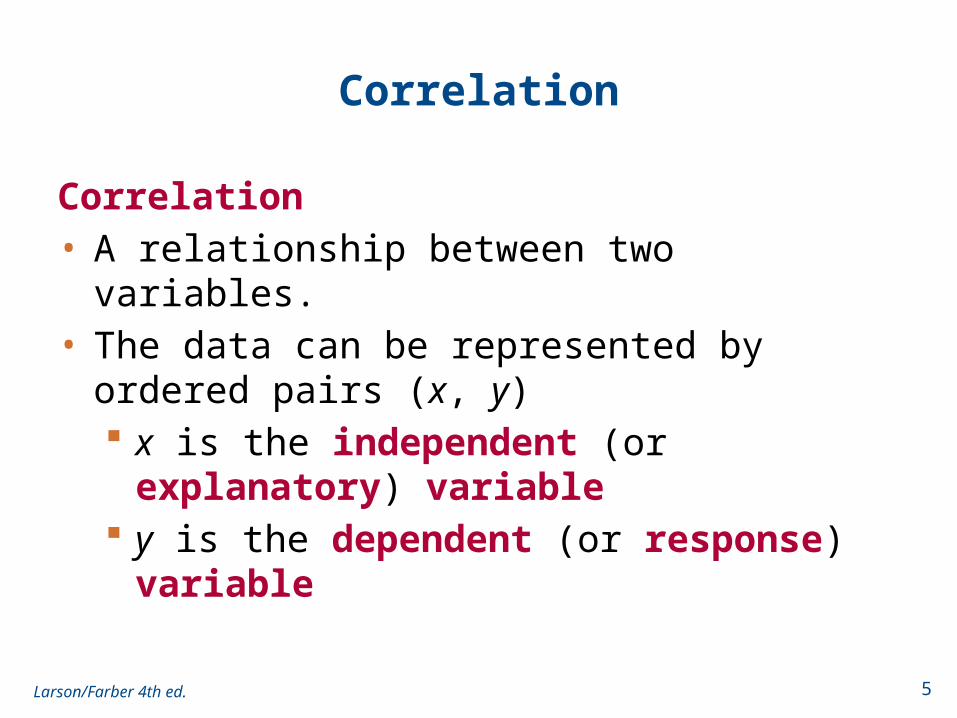
Correlation

Correlation • A relationship between two variables. • The data can be represented by ordered pairs (x, y)

x is the independent (or explanatory) variable y is the dependent (or response) variable


Correlation

x 1 2 3 4 5

y – 4 – 2 – 1 0 2

A scatter plot can be used to determine whether a linear (straight line) correlation exists between two variables.

x

2 4

–2

– 4

y

2

6

Example:


Types of Correlation

x

y

Negative Linear Correlation

x

y

No Correlation

x

y

Positive Linear Correlation

x

y

Nonlinear Correlation

As x increases, y tends to decrease.

As x increases, y tends to increase.


Example: Constructing a Scatter Plot

A marketing manager conducted a study to determine whether there is a linear relationship between money spent on advertising and company sales. The data are shown in the table. Display the data in a scatter plot and determine whether there appears to be a positive or negative linear correlation or no linear correlation.

Advertisingexpenses,($1000), x

Companysales

($1000), y2.4 2251.6 1842.0 2202.6 2401.4 1801.6 1842.0 1862.2 215


Solution: Constructing a Scatter Plot

x

y

Advertising expenses(in thousands of

dollars)

Com

pany

sal

es(i

n th

ousa

nds

of

dolla

rs)

Appears to be a positive linear correlation. As the advertising expenses increase, the sales tend to increase.


Example: Constructing a Scatter Plot Using Technology

Old Faithful, located in Yellowstone National Park, is the world’s most famous geyser. The duration (in minutes) of several of Old Faithful’s eruptions and the times (in minutes) until the next eruption are shown in the table. Using a TI-83/84, display the data in a scatter plot. Determine the type of correlation.

Durationx

Time,y

Durationx

Time,y

1.8 56 3.78 79

1.82 58 3.83 85

1.9 62 3.88 80

1.93 56 4.1 89

1.98 57 4.27 90

2.05 57 4.3 89

2.13 60 4.43 89

2.3 57 4.47 86

2.37 61 4.53 89

2.82 73 4.55 86

3.13 76 4.6 92

3.27 77 4.63 91

3.65 77


Solution: Constructing a Scatter Plot Using Technology

• Enter the x-values into list L1 and the y-values into list L2.

• Use Stat Plot to construct the scatter plot.STAT > Edit… STATPLOT

From the scatter plot, it appears that the variables have a positive linear correlation.


1 550

100

Correlation Coefficient

Correlation coefficient• A measure of the strength and the direction of a linear

relationship between two variables. • The symbol r represents the sample correlation

coefficient. • A formula for r is

• The population correlation coefficient is represented by ρ (rho).

2 22 2

n xy x yr

n x x n y y

n is the number of data pairs


Correlation Coefficient

• The range of the correlation coefficient is -1 to 1.

-1 0 1

If r = -1 there is a perfect negative

correlation

If r = 1 there is a perfect positive

correlation

If r is close to 0 there is no linear

correlation


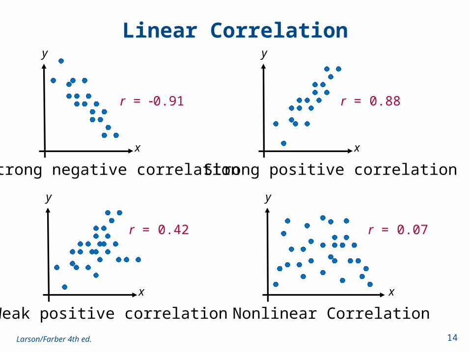
Linear Correlation

Strong negative correlation

Weak positive correlation

Strong positive correlation

Nonlinear Correlation

x

y

x

y

x

y

x

y

r = 0.91 r = 0.88

r = 0.42 r = 0.07


Calculating a Correlation Coefficient

1. Find the sum of the x-values.

2. Find the sum of the y-values.

3. Multiply each x-value by its corresponding y-value and find the sum.

x

y

xy

In Words In Symbols


Calculating a Correlation Coefficient

4. Square each x-value and find the sum.

5. Square each y-value and find the sum.

6. Use these five sums to calculate the correlation coefficient.

2x

2y

2 22 2

n xy x yr

n x x n y y

In Words In Symbols


Example: Finding the Correlation Coefficient

Calculate the correlation coefficient for the advertising expenditures and company sales data. What can you conclude?


Companysales

($1000), y2.4 2251.6 1842.0 2202.6 2401.4 1801.6 1842.0 1862.2 215


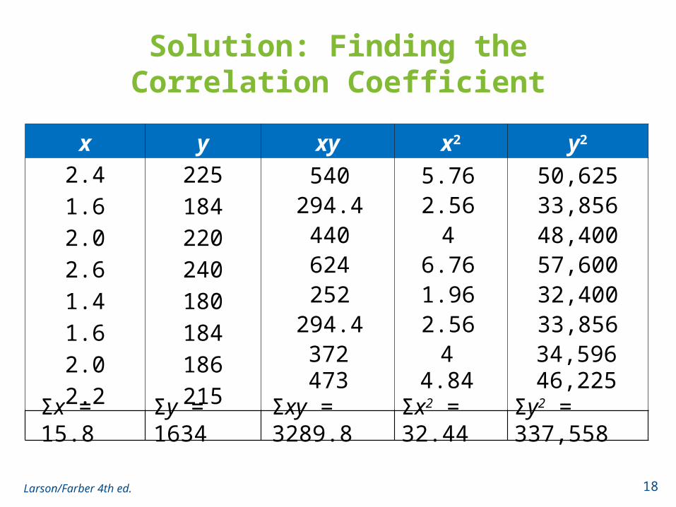
Solution: Finding the Correlation Coefficient

x y xy x2 y2

2.4 2251.6 1842.0 2202.6 2401.4 1801.6 1842.0 1862.2 215

540294.4440624252

294.4372473

5.762.56

46.761.962.56

44.84

50,62533,85648,40057,60032,40033,85634,59646,225

Σx = 15.8 Σy = 1634 Σxy = 3289.8 Σx2 = 32.44 Σy2 = 337,558


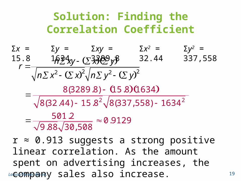
Solution: Finding the Correlation Coefficient

2 22 2

n xy x yr

n x x n y y

2 2

8(3289.8) 15.8 1634

8(32.44) 15.8 8(337,558) 1634

501.2 0.91299.88 30,508

Σx = 15.8 Σy = 1634 Σxy = 3289.8 Σx2 = 32.44 Σy2 = 337,558

r ≈ 0.913 suggests a strong positive linear correlation. As the amount spent on advertising increases, the company sales also increase.


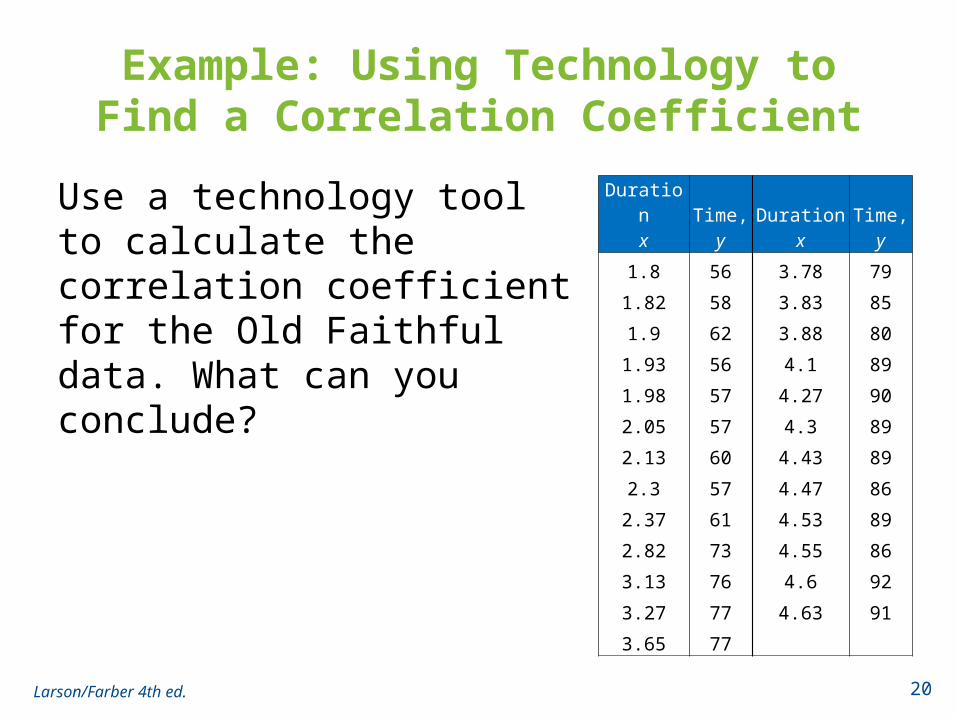
Example: Using Technology to Find a Correlation Coefficient

Use a technology tool to calculate the correlation coefficient for the Old Faithful data. What can you conclude?

Durationx

Time,y

Durationx

Time,y

1.8 56 3.78 79

1.82 58 3.83 85

1.9 62 3.88 80

1.93 56 4.1 89

1.98 57 4.27 90

2.05 57 4.3 89

2.13 60 4.43 89

2.3 57 4.47 86

2.37 61 4.53 89

2.82 73 4.55 86

3.13 76 4.6 92

3.27 77 4.63 91

3.65 77


Solution: Using Technology to Find a Correlation Coefficient

STAT > CalcTo calculate r, you must first enter the DiagnosticOn command found in the Catalog menu

r ≈ 0.979 suggests a strong positive correlation.


Using a Table to Test a Population Correlation Coefficient ρ

• Once the sample correlation coefficient r has been calculated, we need to determine whether there is enough evidence to decide that the population correlation coefficient ρ is significant at a specified level of significance.

• Use Table 11 in Appendix B.• If |r| is greater than the critical value, there is enough

evidence to decide that the correlation coefficient ρ is significant.



• Determine whether ρ is significant for five pairs of data (n = 5) at a level of significance of α = 0.01.

• If |r| > 0.959, the correlation is significant. Otherwise, there is not enough evidence to conclude that the correlation is significant.

Number of pairs of data in sample

level of significance



1. Determine the number of pairs of data in the sample.

2. Specify the level of significance.

3. Find the critical value.

Determine n.

Identify .

Use Table 11 in Appendix B.

In Words In Symbols



In Words In Symbols

4. Decide if the correlation is significant.

5. Interpret the decision in the context of the original claim.

If |r| > critical value, the correlation is significant. Otherwise, there is not enough evidence to support that the correlation is significant.


Example: Using a Table to Test a Population Correlation Coefficient ρ

Using the Old Faithful data, you used 25 pairs of data to find r ≈ 0.979. Is the correlation coefficient significant? Use α = 0.05.

Durationx

Time,y

Durationx

Time,y

1.8 56 3.78 79

1.82 58 3.83 85

1.9 62 3.88 80

1.93 56 4.1 89

1.98 57 4.27 90

2.05 57 4.3 89

2.13 60 4.43 89

2.3 57 4.47 86

2.37 61 4.53 89

2.82 73 4.55 86

3.13 76 4.6 92

3.27 77 4.63 91

3.65 77


Solution: Using a Table to Test a Population Correlation Coefficient ρ

• n = 25, α = 0.05• |r| ≈ 0.979 > 0.396• There is enough evidence

at the 5% level of significance to conclude that there is a significant linear correlation between the duration of Old Faithful’s eruptions and the time between eruptions.


Hypothesis Testing for a Population Correlation Coefficient ρ

• A hypothesis test can also be used to determine whether the sample correlation coefficient r provides enough evidence to conclude that the population correlation coefficient ρ is significant at a specified level of significance.

• A hypothesis test can be one-tailed or two-tailed.


Hypothesis Testing for a Population Correlation Coefficient ρ

• Left-tailed test

• Right-tailed test

• Two-tailed test

H0: ρ 0 (no significant negative correlation)

Ha: ρ < 0 (significant negative correlation)

H0: ρ 0 (no significant positive correlation)

Ha: ρ > 0 (significant positive correlation)

H0: ρ = 0 (no significant correlation)

Ha: ρ 0 (significant correlation)


The t-Test for the Correlation Coefficient

• Can be used to test whether the correlation between two variables is significant.

• The test statistic is r • The standardized test statistic

follows a t-distribution with d.f. = n – 2.• In this text, only two-tailed hypothesis tests for ρ are

considered.

212

r

r rtr

n


Using the t-Test for ρ

1. State the null and alternative hypothesis.

2. Specify the level of significance.

3. Identify the degrees of freedom.

4. Determine the critical value(s) and rejection region(s).

State H0 and Ha.

Identify .

d.f. = n – 2.


In Words In Symbols


Using the t-Test for ρ

5. Find the standardized test statistic.

6. Make a decision to reject or fail to reject the null hypothesis.

7. Interpret the decision in the context of the original claim.

In Words In Symbols

If t is in the rejection region, reject H0. Otherwise fail to reject H0.

212

rtr

n


Example: t-Test for a Correlation Coefficient

Previously you calculated r ≈ 0.9129. Test the significance of this correlation coefficient. Use α = 0.05.


Companysales

($1000), y2.4 2251.6 1842.0 2202.6 2401.4 1801.6 1842.0 1862.2 215


t0-2.447

0.025

2.447

0.025

Solution: t-Test for a Correlation Coefficient

• H0:

• Ha:

• • d.f. = • Rejection Region:

• Test Statistic:

0.058 – 2 = 6

2

0.91295.478

1 (0.9129)

8 2

t

ρ = 0ρ ≠ 0

-2.447 2.447

5.478

• Decision:At the 5% level of significance, there is enough evidence to conclude that there is a significant linear correlation between advertising expenses and company sales.

Reject H0


Correlation and Causation

• The fact that two variables are strongly correlated does not in itself imply a cause-and-effect relationship between the variables.

• If there is a significant correlation between two variables, you should consider the following possibilities.1. Is there a direct cause-and-effect relationship

between the variables?• Does x cause y?


Correlation and Causation

2. Is there a reverse cause-and-effect relationship between the variables?• Does y cause x?

3. Is it possible that the relationship between the variables can be caused by a third variable or by a combination of several other variables?

4. Is it possible that the relationship between two variables may be a coincidence?


Section 9.1 Summary

• Introduced linear correlation, independent and dependent variables and the types of correlation

• Found a correlation coefficient• Tested a population correlation coefficient ρ using a

table• Performed a hypothesis test for a population

correlation coefficient ρ• Distinguished between correlation and causation


Section 9.2

Linear Regression



• Find the equation of a regression line• Predict y-values using a regression equation


Regression lines

• After verifying that the linear correlation between two variables is significant, next we determine the equation of the line that best models the data (regression line).

• Can be used to predict the value of y for a given value of x.

x

y


Residuals

Residual• The difference between the observed y-value and the

predicted y-value for a given x-value on the line.

For a given x-value,

di = (observed y-value) – (predicted y-value)

x

y

}d1

}d2

d3{d4{ }d5

d6{

Predicted y-value

Observed y-value


Regression line (line of best fit)• The line for which the sum of the squares of the

residuals is a minimum. • The equation of a regression line for an independent

variable x and a dependent variable y isŷ = mx + b

Regression Line

Predicted y-value for a given x-value

Slopey-intercept


The Equation of a Regression Line

• ŷ = mx + b where

• is the mean of the y-values in the data• is the mean of the x-values in the data• The regression line always passes through the point

22

n xy x ym

n x x

y xb y mx mn n

y

x

,x y


Example: Finding the Equation of a Regression Line

Find the equation of the regression line for the advertising expenditures and company sales data.


Companysales

($1000), y2.4 2251.6 1842.0 2202.6 2401.4 1801.6 1842.0 1862.2 215


Solution: Finding the Equation of a Regression Line

x y xy x2 y2

2.4 2251.6 1842.0 2202.6 2401.4 1801.6 1842.0 1862.2 215

540294.4440624252

294.4372473

5.762.56

46.761.962.56

44.84

50,62533,85648,40057,60032,40033,85634,59646,225

Σx = 15.8 Σy = 1634 Σxy = 3289.8 Σx2 = 32.44 Σy2 = 337,558

Recall from section 9.1:



Σx = 15.8 Σy = 1634 Σxy = 3289.8 Σx2 = 32.44 Σy2 = 337,558

22

n xy x ym

n x x

b y mx

28(3289.8) (15.8)(1634)

8(32.44) 15.8

501.2 50.728749.88

1634 15.8(50.72874)8 8

204.25 (50.72874)(1.975) 104.0607

ˆ 50.729 104.061y x Equation of the regression line



• To sketch the regression line, use any two x-values within the range of the data and calculate the corresponding y-values from the regression line.

ˆ 50.729 104.061y x

1.2 1.4 1.6 1.8 2 2.2 2.4 2.6 2.8160

180

200

220

240

260

x

Advertising expenses(in thousands of dollars)

Com

pany

sal

es(i

n th

ousa

nds

of d

olla

rs) y


Example: Using Technology to Find a Regression Equation

Use a technology tool to find the equation of the regression line for the Old Faithful data.

Durationx

Time,y

Durationx

Time,y

1.8 56 3.78 79

1.82 58 3.83 85

1.9 62 3.88 80

1.93 56 4.1 89

1.98 57 4.27 90

2.05 57 4.3 89

2.13 60 4.43 89

2.3 57 4.47 86

2.37 61 4.53 89

2.82 73 4.55 86

3.13 76 4.6 92

3.27 77 4.63 91

3.65 77


Solution: Using Technology to Find a Regression Equation


550

100

1

Example: Predicting y-Values Using Regression Equations

The regression equation for the advertising expenses (in thousands of dollars) and company sales (in thousands of dollars) data is ŷ = 50.729x + 104.061. Use this equation to predict the expected company sales for the following advertising expenses. (Recall from section 9.1 that x and y have a significant linear correlation.)

1. 1.5 thousand dollars




Solution: Predicting y-Values Using Regression Equations

ŷ = 50.729x + 104.061


When the advertising expenses are $1500, the company sales are about $180,155.

ŷ =50.729(1.5) + 104.061 ≈ 180.155



ŷ =50.729(1.8) + 104.061 ≈ 195.373


Solution: Predicting y-Values Using Regression Equations



ŷ =50.729(2.5) + 104.061 ≈ 230.884

Prediction values are meaningful only for x-values in (or close to) the range of the data. The x-values in the original data set range from 1.4 to 2.6. So, it wouldnot be appropriate to use the regression line to predictcompany sales for advertising expenditures such as 0.5 ($500) or 5.0 ($5000).


Section 9.2 Summary

• Found the equation of a regression line• Predicted y-values using a regression equation


Section 9.3

Measures of Regression and Prediction Intervals



• Interpret the three types of variation about a regression line

• Find and interpret the coefficient of determination• Find and interpret the standard error of the estimate

for a regression line• Construct and interpret a prediction interval for y


Variation About a Regression Line

• Three types of variation about a regression line Total variation Explained variation Unexplained variation

• To find the total variation, you must first calculate The total deviation The explained deviation The unexplained deviation



iy yîy y

î iy y

(xi, ŷi)

x

y (xi, yi)

(xi, yi)

Unexplained deviation

î iy yTotal

deviationiy y Explained

deviationîy y

y

x

Total Deviation =

Explained Deviation =

Unexplained Deviation =


Total variation • The sum of the squares of the differences between the

y-value of each ordered pair and the mean of y.

Explained variation • The sum of the squares of the differences between

each predicted y-value and the mean of y.


2iy y Total variation =

Explained variation = 2ˆiy y


Unexplained variation • The sum of the squares of the differences between the

y-value of each ordered pair and each corresponding predicted y-value.


2ˆi iy y Unexplained variation =

The sum of the explained and unexplained variation is equal to the total variation.


Total variation = Explained variation + Unexplained variation

Coefficient of Determination

Coefficient of determination• The ratio of the explained variation to the total

variation.• Denoted by r2

2 Explained variationTotal variation

r


Example: Coefficient of Determination

22 (0.913)

0.834

r

About 83.4% of the variation in the company sales can be explained by the variation in the advertising expenditures. About 16.9% of the variation is unexplained.

The correlation coefficient for the advertising expenses and company sales data as calculated in Section 9.1 isr ≈ 0.913. Find the coefficient of determination. What does this tell you about the explained variation of the data about the regression line? About the unexplained variation?Solution:


The Standard Error of Estimate

Standard error of estimate

• The standard deviation of the observed yi -values about the predicted ŷ-value for a given xi -value.

• Denoted by se.

• The closer the observed y-values are to the predicted

y-values, the smaller the standard error of estimate will be.

2( )ˆ2

i ie

y ys

n

n is the number of ordered pairs in the data set


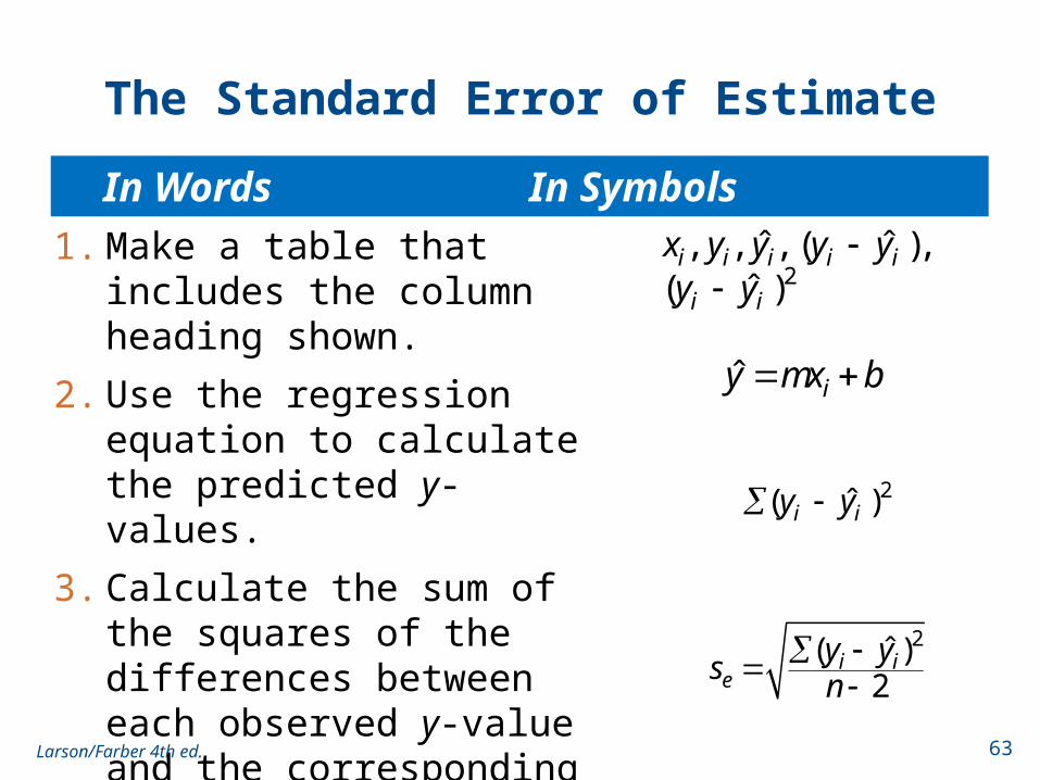
The Standard Error of Estimate

2

, , , ( ), ˆ ˆ( )ˆ

i i i i i

i i

x y y y yy y

1. Make a table that includes the column heading shown.

2. Use the regression equation to calculate the predicted y-values.

3. Calculate the sum of the squares of the differences between each observed y-value and the corresponding predicted y-value.

4. Find the standard error of estimate.

ˆ iy mx b

2 ( )ˆi iy y

2( )ˆ2

i ie

y ys

n

In Words In Symbols


Example: Standard Error of Estimate

The regression equation for the advertising expenses and company sales data as calculated in section 9.2 is

ŷ = 50.729x + 104.061

Find the standard error of estimate.

Solution:Use a table to calculate the sum of the squared differences of each observed y-value and the corresponding predicted y-value.


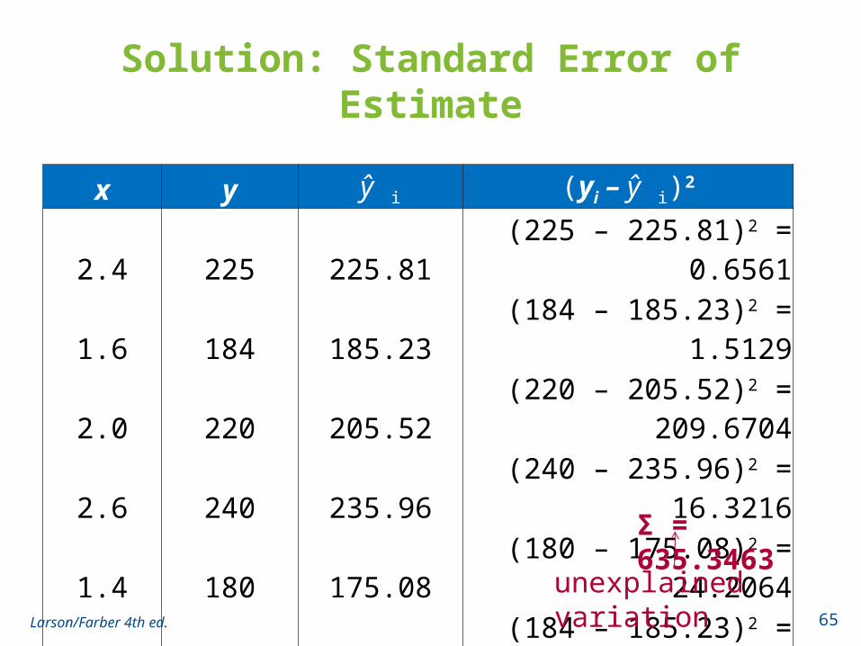
Solution: Standard Error of Estimate

x y ŷ i (yi – ŷ i)2

2.4 225 225.81 (225 – 225.81)2 = 0.65611.6 184 185.23 (184 – 185.23)2 = 1.51292.0 220 205.52 (220 – 205.52)2 = 209.67042.6 240 235.96 (240 – 235.96)2 = 16.32161.4 180 175.08 (180 – 175.08)2 = 24.20641.6 184 185.23 (184 – 185.23)2 = 1.51292.0 186 205.52 (186 – 205.52)2 = 381.03042.2 215 215.66 (215 – 215.66)2 = 0.4356

Σ = 635.3463

unexplained variation65Larson/Farber 4th ed.

Solution: Standard Error of Estimate

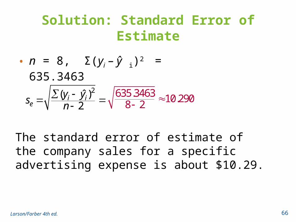
• n = 8, Σ(yi – ŷ i)2 = 635.3463

2( )ˆ2

i ie

y ys

n

The standard error of estimate of the company sales for a specific advertising expense is about $10.29.

635.3463 10.2908 2


Prediction Intervals

• Two variables have a bivariate normal distribution if for any fixed value of x, the corresponding values of y are normally distributed and for any fixed values of y, the corresponding x-values are normally distributed.


Prediction Intervals

• A prediction interval can be constructed for the true value of y.

• Given a linear regression equation ŷ = mx + b and x0, a specific value of x, a c-prediction interval for y is

ŷ – E < y < ŷ + E where

• The point estimate is ŷ and the margin of error is E. The probability that the prediction interval contains y is c.

202 2

( )11( )c e

n x xE t s

n n x x


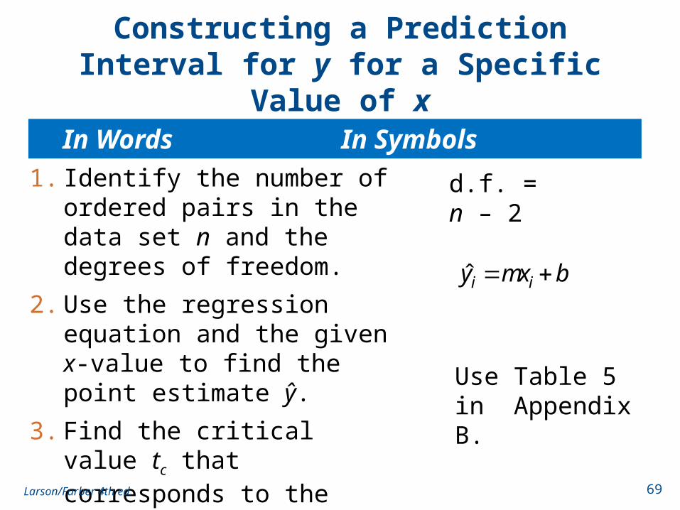
Constructing a Prediction Interval for y for a Specific Value of x

1. Identify the number of ordered pairs in the data set n and the degrees of freedom.

2. Use the regression equation and the given x-value to find the point estimate ŷ.

3. Find the critical value tc that corresponds to the given level of confidence c.

ˆi iy mx b


In Words In Symbols

d.f. = n – 2


Constructing a Prediction Interval for y for a Specific Value of x

4. Find the standard error of estimate se.

5. Find the margin of error E.

6. Find the left and right endpoints and form the prediction interval.

In Words In Symbols2( )ˆ

2i i

ey y

sn

2

02 2

( )11( )c e

n x xE t s

n n x x

Left endpoint: ŷ – E Right endpoint: ŷ + E Interval: ŷ – E < y < ŷ + E


Example: Constructing a Prediction Interval

Construct a 95% prediction interval for the company sales when the advertising expenses are $2100. What can you conclude?

Recall, n = 8, ŷ = 50.729x + 104.061, se = 10.290

Solution:Point estimate: ŷ = 50.729(2.1) + 104.061 ≈ 210.592

Critical value:d.f. = n –2 = 8 – 2 = 6 tc = 2.447

215.8, 32.44, 1.975x x x


Solution: Constructing a Prediction Interval

0

2

2

2

2 2

1 8(2.1 1.975)(2.447)(10.290) 1 26.8578 8(32.44) (15

( )

8)

1

.

1( )c e

n x xE t s

n n x x

Left Endpoint: ŷ – E Right Endpoint: ŷ + E

183.735 < y < 237.449

210.592 – 26.857≈ 183.735

210.592 + 26.857≈ 237.449

You can be 95% confident that when advertising expenses are $2100, the company sales will be between $183,735 and $237,449.


Section 9.3 Summary

• Interpreted the three types of variation about a regression line

• Found and interpreted the coefficient of determination

• Found and interpreted the standard error of the estimate for a regression line

• Constructed and interpreted a prediction interval for y


Section 9.4

Multiple Regression



• Use technology to find a multiple regression equation, the standard error of estimate and the coefficient of determination

• Use a multiple regression equation to predict y-values


Multiple Regression Equation

• In many instances, a better prediction can be found for a dependent (response) variable by using more than one independent (explanatory) variable.

• For example, a more accurate prediction for the company sales discussed in previous sections might be made by considering the number of employees on the sales staff as well as the advertising expenses.


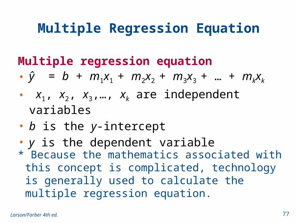
Multiple Regression Equation

Multiple regression equation • ŷ = b + m1x1 + m2x2 + m3x3 + … + mkxk

• x1, x2, x3,…, xk are independent variables

• b is the y-intercept• y is the dependent variable

* Because the mathematics associated with this concept is complicated, technology is generally used to calculate the multiple regression equation.


Example: Finding a Multiple Regression Equation

A researcher wants to determine how employee salaries at a certain company are related to the length of employment, previous experience, and education. The researcher selects eight employees from the company and obtains the data shown on the next slide. Use Minitab to find a multiple regression equation that models the data.


Example: Finding a Multiple Regression Equation

Employee Salary, yEmployment

(yrs), x1

Experience (yrs), x2

Education (yrs), x3

A 57,310 10 2 16B 57,380 5 6 16C 54,135 3 1 12D 56,985 6 5 14E 58,715 8 8 16F 60,620 20 0 12G 59,200 8 4 18H 60,320 14 6 17


Solution: Finding a Multiple Regression Equation

• Enter the y-values in C1 and the x1-, x2-, and x3-values in C2, C3 and C4 respectively.

• Select “Regression > Regression…” from the Stat menu.

• Use the salaries as the response variable and the remaining data as the predictors.


Solution: Finding a Multiple Regression Equation

The regression equation is ŷ = 49,764 + 364x1 + 228x2 + 267x3


Predicting y-Values

• After finding the equation of the multiple regression line, you can use the equation to predict y-values over the range of the data.

• To predict y-values, substitute the given value for each independent variable into the equation, then calculate ŷ.


Example: Predicting y-Values

Use the regression equation ŷ = 49,764 + 364x1 + 228x2 + 267x3

to predict an employee’s salary given 12 years of current employment, 5 years of experience, and 16 years of education.

Solution:ŷ = 49,764 + 364(12) + 228(5) + 267(16) = 59,544

The employee’s predicted salary is $59,544.


Section 9.4 Summary

• Used technology to find a multiple regression equation, the standard error of estimate and the coefficient of determination

• Used a multiple regression equation to predict y-values


Chapter 9 Correlation and Regression 1 Larson/Farber 4th ed.

Documents

Transcript of Chapter 9 Correlation and Regression 1 Larson/Farber 4th ed.