Chapter 8

Theory of Generalized

Randles-Ershler Admittance of

Rough and Finite Fractal

Electrode

“So oft in theologic wars,

The disputants, I ween,

Rail on in utter ignorance

Of what each other mean,

And prate about an Elephant

Not one of them has seen ! ”

- John Godfrey Saxe (The Blind Men and the Elephant)

269

270

Abstract

Theory of generalized Randles-Ershler admittance in presence of supporting elec-

trolyte is developed for arbitrary rough electrode. The model incorporates various

physical components : the semi-infinite diffusion admittance, the charge trans-

fer reaction resistance Rct, and the capacitance Cd of the EDL. The dynamics of

the system is represented through Bode and Nyquist response and is found to de-

pend on phenomenological length scales- diffusion length (D/ω)1/2, and the charge

transfer layer thickness Lct, and their coupling with various roughness features.

Two characteristic times scale, finite charge transfer time τd = L2ct/D, and electric

double layer charging time τc = RctCd are identified. The whole electrochemical

response of the electrode is found to consists of four regimes: (1) diffusion con-

trolled (classical Warburg), (2) anomalous Warburg behavior, (3) charge transfer

controlled (Faradaic) and (4) double layer controlled (capacitive). Results are ob-

tained that can be applied both for stochastic and deterministic surface profile.

The randomness in electrode roughness is characterized through statistical prop-

erty of structure factor. A detailed analysis of roughness effect is carried out for

a finite self-affine fractal electrode. The influence of roughness is shown through

surface morphological parameters: fractal dimension DH , smallest length scale

of roughness ℓ and width of interface µ. The phase clearly marks four regimes:

(1) low frequency classical Warburg impedance with phase angle Φ(ω) = 45, (2)

followed by anomalous Warburg for intermediate frequencies where phase angle

Φ(ω) > 45, (3) quasi-reversible charge transfer controlled where the phase angle

is 0 < Φ(ω) < 45 and (4) crossover to purely capacitive controlled with phase

angle Φ(ω) = 90.

271

272

1 Introduction

The transport properties and the kinetics in relation to the morphological charac-

teristic are found to have increasing effects on the electrochemical response and its

applications lies at the heart of modern day electrochemical devices like batteries

[1, 2], fuel cells [3, 4], electrochromic smart windows [5], ion exchange membranes

[6], solar cells[7], capacitive deionization cells [8], and supercapacitors [8]. The

transport of charge and kinetics of an electrochemical reaction taking place at the

electrode is a very general problem in science and technology [9, 10, 11, 12]. This

problem also arise in nanostructured semiconductor electrodes [13], electrochromic

films [5, 14], nanoporous polymer membranes [6] and ion intercalation in nanos-

tructured materials [2, 15] which have ubiquitous electrode geometry.

It is well known that the transport properties and the kinetics in relation

to the geometrical morphological characteristic like non-uniformities of the sur-

face, viz., roughness [16, 17] and porosity are found to affect the electrochemical

response. While modeling the electrochemical response of rough electrode is con-

sidered mathematically difficult and usually avoided, roughness of electrode have

resulted in many anomalous behavior, viz., constant phase element (CPE) [18],

anomalous Warburg [19, 20] and anomalous Gerischer [21, 22] behavior. Under-

standing the influence of electrode geometry in relation to mass transport, its effect

on the kinetics and electrochemical response has been the longstanding goal of var-

ious studies. On the other hand various process like diffusion [9, 23, 24], adsorption

[10, 11], heterogeneous catalysis [25, 26], nmr relaxation [27], fluorescence quench-

ing [28], enzyme kinetics [28], diffusion limited adsorption/aggregation [24, 29] and

electrochemistry of disordered system [30] are affected by the transport of ion from

the bulk and across the interface making this problem of very wide applications.

Experimental investigation are made employing transient measurements like

voltammetry [31] and electrochemical impedance spectroscopy (EIS) [4, 32] to un-

derstand the possible role of roughness in the the problem of charge transport and

273

kinetics of the electrochemical reaction. Particular EIS is a powerful technique

since it involve measurement of a process from micro- to nanoseconds in a sin-

gle experiment. Various time scales and relaxation process can be differentiated

through impedance measurement. The information obtained from EIS may be

used to investigate the type of partial process like charge transfer, diffusion and

adsorption/desorption and distinguish microscopic laws that governs the mecha-

nism of charge transfer [5], adsorption isotherm and anomalous properties. But

the interpretation of impedance data is considered problematic and often associ-

ated with difficulties. Understanding the underlying mechanism in interpretation

is considered as utmost important and this may be achieve by developing mathe-

matical model incorporating the roughness of electrode. The frequency response

of a rough electrode depends on the electrochemical regime. Two regimes in elec-

trochemical context, particularly important are: (1) the kinetic controlled and (2)

the mass controlled regimes.

Broadly speaking the electrochemical process at the electrode may be classified

into two: Faradaic and non-Faradaic. A Faradic process is defined as one in

which the amount of chemical reaction occurring is directly proportional to the

amount of charge passing across the electrode i.e., interfacial oxidation and/or

reduction. A typical non-Faradaic process is the charging of the EDL capacitance

of a blocking electrode. These two process have different implication. Faradaic

reactions are important features of electrochemical cells like fuel cells and batteries.

The charging and discharging of batteries essentially depends on the Faradaic

reaction taking place. The non-Faradaic process like charging have important

effect in electric double layer capacitance and in presence of Faradaic reaction can

increase the charge stored by pseudo-capacitance.

The classical theories developed for understanding electrode kinetics [33, 34,

36, 37, 38, 39, 40, 41, 42, 43, 45, 46], couple ion transport in the electrolyte phase to

either to the Faradaic charge transfer reaction or double layer capacitive charging.

One of the earliest classic studies on the kinetics of charge transfer was made

274

by Randles. His theory of kinetics of electrochemical reaction is based on the

solution of diffusion equation in a semi-infinite, one dimensional domain satisfying

the Butler-Volmer’s current-overpotential equation [46]. Delahay and coworker

also developed theories of the electric double layer impedance with finite charge

transfer [36, 37]. Since then many modified theories has been made accounting

adsorptions [35, 44], multi-step reactions [35, 40] and coupling of various quantities

[35, 36, 43].

The assumption that the two process: Faradaic and non-Faradaic are inde-

pendent of each other may be erroneous and this is much more serious for elec-

trochemical cells where both process may occurs simultaneously. The problem of

mass transport to and from interface in presence of Faradaic reactions is affected

by the nature of the coupled chemical reaction in the solution. In general three

factor [46] which affects the kinetics of an electrode reaction are, (1) the rate of

the electrode process, (2) the rate of diffusion of the reactant and product, and

(3) the ohmic resistance of the electrolyte. So in analyzing an electrochemical cell

one has to separate individual components or either minimized the other two in

order to arrive to a meaningful conclusion of the underlying mechanism. However,

the physics of the separation of the impedance into Faradaic and charging con-

tributions remains not sufficiently clear. This concerns especially in the case of

rough and porous electrodes. The theoretical basis of separation is rather poorly

developed. Recently Bazant and Biesheuvel and coworkers [47] have developed a

theory for the diffuse layer charging and Faradaic reaction for porous electrode.

But the model developed are insufficient for admittance/impedance of rough elec-

trode analysis in presence of charge transfer. Macdonald and coworkers also have

addressed the problem of charge transfer for two identical electrodes separated

by a finite distance [32]. Different cases: supported and unsupported systems

[48], stationary and mobile [49] and fast and slow reaction rates [48] were stud-

ied. Analysis were made using the Nernst-Planck-Poisson equation and using the

Change-Jaffe boundary conditions. But no any consideration on the geometry and

275

morphology of electrode was made.

Theoretically there has been essentially three approaches made to the under-

standing the role of roughness and transport and kinetic phenomena at the inter-

face. First is the equivalent circuit (EC) approach [51], second the scaling approach

[50, 51] and third ab initio approach [53, 54, 55]. The equivalent circuit model ap-

proach are popular due top its simplicity. One of the most widely employed model

is Randles-Ershler equivalent circuit, based on the work of Randles [46] and Er-

shler [52]. It consist of a resistor representing electrolyte resistance in series of a

circuit consisting of a parallel combination of a capacitor representing EDL and

a general impedance consisting the charge transfer resistance and the Warburg

impedance. Randles-Ershler equivalent circuit and modified analogues are exten-

sively used in interpretation of current in fuel cells, kinetics of ion intercalation in

batteries and interpretation EDL charging in modified nano electrodes. However,

the exact theoretical basis of Randles-Ershler equivalent circuit for rough electrode

is not known. It is generally assumed that when a current pulse is applied to an

interface, one part is consumed by the double-layer charging and the other part

is used for an interface electrochemical reaction. A widely employed simplifica-

tion is a priori separation of the total electric current into Faradaic and charging

currents. The weakness of the method of a priori separation of the currents has

been pointed by several workers [39, 56]. Rangarajan [34, 35] pointed out that

the double layer capacity is no “capacity” but is a generalized impedance whose

elements exhibits an involved dependence on various electrochemical process hap-

pening at the interface. Thus the Faradaic process and the charging of EDL are

coupled and a priori separation of the two process as independent component is er-

roneous as usually done in electrical equivalent circuits models and corresponding

Randles-Ershler type circuit. Also one serious drawback of using circuit analysis

is the extraction of kinetic parameters, diffusion coefficient, and other information

tractable from impedance measurements when there is a dynamic interplay of the

various effects, viz., surface roughness, diffusion, charge transfer, ohmic resistance

276

and electric double layer capacitance. At the same time, the role of roughness

in various situation like diffusion limited, electric double layer CPE behavior and

anomalous effects get erroneously included in kinetic measurement. Since there is

no definite intuitive connection between a mechanism by which an electrochemical

process take place and a corresponding equivalent circuit components, relating to

a physical phenomena is very difficult to interpret EIS data purely on basis of

electrical circuit. Fitting the electrochemical response through EC models does

not guarantee the exact correspondence of electrical component to the underlying

electrochemical mechanism[32, 56].

However it is desirable or essential to decouple other effects from roughness

effect and to understanding the role of electrode geometry. This pose a fundamen-

tal and important challenging problem relevant in modern day electrochemical

cells. Thus one must reexamine the premise of traditional Randles-Ershler equiv-

alent circuit as it applies only to physically to an ideal planar electrodes, while

all natural/engineered electrodes are essentially rough or porous. To best of our

knowledge no particular studies has been made to account the roughness of the

electrode and effect on the electrochemical response on the Randles-Ershler level.

Another approach is the scaling approach. Here the admittance of rough elec-

trode is expressed as a power law relation given by

Y (ω) ∼ (jω)γ (1.0.1)

The exponent γ is such that 0 < γ < 1. This behavior is known as constant

phase element (CPE) behavior. Different researcher have tried to explain the CPE

differently, invoking a distribution of relaxation time constants [57], rough/fractal

nature of electrode geometries [17], pore structure [50, 51], non-uniform current-

potential distribution [57, 58] and adsorption/desorption [59, 60]. The theories of

CPE are still unable to explain behavior given by Eq. 1.0.1 observed in various

experiment and the exact origin is still not clear. There are various theories on how

277

the γ is related to roughness [16, 17, 27, 50, 51] of the electrode. Le Mehaute and

Crepy first suggested that the exponent γ is related to the fractal dimension (DH)

of the interface [16]. Before that de Gennes suggested the interrelation between γ

and fractal dimension as γ = (DH − 1)/2 for the problem of diffusion controlled

NMR (nuclear magnetic relaxation) in porous media with DH as fractal dimension

[27]. This result has been obtained for diffusion impedance of a fractal interface

by Nyikos and Pajkossy for Koch electrode [17].

The third approach is the ab initio approach. In this approach the problem of

mass transfer across or to an irregular interface is solved under the Fick’s law of

diffusion using the geometry dependent flux arriving at the interface. Appropriate

boundary condition are used to solve the formulated boundary value problem rig-

orously. Ab initio approach are usually considered difficult and usually avoided.

Kant and coworkers have solved the problem of charge transfer taking at a rough

electrode under partial diffusion limited process on rough electrode [53, 54, 55].

An elegant formalism based on the diffusion adopting ab initio methodology has

been successfully developed to understand the influence of roughness on the elec-

trochemical response of rough electrode. Recently theories for diffusion limited

charge transfer process (Warburg [64], Gerischer [21] and Anson [65, 66]), quasi-

reversible charge transfer admittance on fractal electrodes [68, 69] and the anoma-

lous Warburg admittance [70] on rough electrode modeled as realistic fractals have

also been developed to understand the problem where diffusion and heterogeneous

charge transfer kinetics occurs. All these theoretical studies have not only pro-

vided new insights into the complex influence of roughness in the heterogeneous

charge transfer reaction but also indicate the advantages over other approaches in

capturing various roughness dependent anomalous effects and transition leading

to classical planar behavior. The analytical theories based on ab initio method-

ology can in-fact be generalized incorporating one or more process. Different

generalizations of the Randles-Ershler model for diverse electrode systems exist

in literatures [35, 72, 71]. But none of them address or incorporate the effect of

278

electrode geometry on the Randles-Ershler response at the ab initio level.

In this work we address the problem of charge transfer and kinetics of electro-

chemical reaction including the double layer charging current on rough electrode

at the Randles-Ershler level. As a simplification we used the concept of excess

supporting electrolyte and thus neglecting or consider the ohmic resistance of

electrolyte small so that it has no influence on the response of the system. The

generalized Randles-Ershler problem making no use of concept of supporting elec-

trolyte excess and the possible influence of ohmic resistance will be presented in

another communication. The goal of this paper is to develop a theory of admit-

tance to understand the role of electrode roughness, diffusion and heterogeneous

kinetics taking place at a rough electrode in presence of capacitive electric double

layer charging. The paper is organized as follows: first we conceived the problem of

charge transfer due to diffusion of ions in presence of EDL as Randles-Ershler prob-

lem of single step reaction in presence of excess supporting electrolyte. We used

the Butler-Volmer (current-overpotential) equation as a standard model for charge

transfer kinetics but with EDL capacitive charging current correction. Modeling

the electrode as realistic random fractal we solve the boundary value problem and

generalized admittance are obtained for deterministic surface as-well for stochastic

surface expressing as a function of surface structure function. We analyzed the

effect of charge transfer resistance, electric double layer capacitance in relation

to roughness of electrode on the admittance and phase. Both Nyquist and Bode

analysis are presented. Finally we conclude with results and discussion.

Figure 8.1 shows the schematic picture of problem of charge transfer on rough

electrode with electric double layer charging. The charge transfer reaction O(Sol)+

ne−kfkbR(Sol) is assume to occur in a region of thickness LCT which we called

charge transfer layer thickness, which depends on the charge transfer resistance

RCT . The mass transport is purely diffusive and introduce a frequency depen-

dent phenomenological length LD ∼√D/ω depending on the diffusion coefficient

D. The random roughness profile is characterized by four fractal morphological

279

Figure 8.1: Schematic picture of semi-infinite Randles-Ershler problem on a roughelectrode. The inset shows the classical Randles equivalent circuit with variouscomponents with corresponding currents.

characteristics, viz., the width (h) of the interface which is related to the strength

of fractality (µ), lower cutoff length scale (l), upper cutoff length scale (L) and

the fractal dimension (DH). The inset in the picture shows the classical Randles

equivalent circuit for planar electrode under supported conditions (neglecting the

ohmic resistance of the electrolyte). It consists of a series resistor representing

charge transfer resistance (RCT ) with Warburg impedance in parallel to a capaci-

tor representing the electric double layer capacitor (Cd). Here i represent the total

current and ic and if represent the non-Faradaic electric double layer charging ca-

pacitive current and Faradaic charge transfer current at the interface

2 Mathematical Formulation

2.1 Diffusion towards and from Rough electrode

In this section we formulate the problem of charge transfer on rough electrode

in presence of electric double charging conceiving it as Randles-Ershler problem

of electrode kinetics. Let us consider the charge transfer occurs in a single step

280

reversible electrochemical reaction whose mass transfer is purely controlled by

process of diffusion

O(Sol) + ne−kfkbR(Sol) (2.1.1)

The corresponding mass transfer diffusion equation may be written as

∂δCα(r, t)

∂t= Dα∇2δCα(r, t) (2.1.2)

where, ∂δCα(r, t) = δCα(r, t)−C0α(r, t) is the difference in concentration of species

α, C0α(r, t) is the bulk concentration, Dα is the bulk molecular diffusion coefficient,

kf and kb are the forward and backward reaction rate constant.

2.2 Linearized Current-Overpotential Equation with Dou-

ble layer Charging

The current arriving at the irregular boundary may be obtained from the classical

Bulter-Volmer (current-overpotential) equation. Now for a rough electrode under-

going quasi-reversible reaction due to diffusion of ions, the current at the electrode

in presence of EDL is determined not only by mass transfer and charge transfer ki-

netics but also depends on the capacitive current charging the EDL. The linearized

Butler-Volmer equation for small overpotential with EDL capacitive charging is

[55, 69]i(ζ, t)

i0=δC0(ζ, t)

C0O

− δCR(ζ, t)

C0R

+ nfη(t) +

(Cd

i0

)dη(t)

dt(2.2.1)

where i(ζ, t) is the local surface profile dependent current density, i0 is the exchange

current density across the interface, n is the number of electron transfered in redox

reaction 2.1.1, η(t) is the input potential, f = F/RT and Cd is the electric double

layer capacitance. Here F is the Faraday’s constant, R the universal gas constant,

T is the absolute temperature and δCα(ζ) is the difference between the bulk and

surface concentration. This boundary condition was first obtained by Delahay and

281

coworkers [37]. At an initial time t = 0, the concentration of diffusing species is

δCα(r, t = 0) = 0 (2.2.2)

and far from the electrode the bulk concentration is given by

δCα(r∥, z → 0, t) = 0 (2.2.3)

The local current density due to diffusional current at a point ζ(x, y) is given by

i(ζ, t) = nFD0∂nδCO(ζ, t) (2.2.4)

where DO is the diffusion coefficient of oxidized species and ∂n = n.∇ represents

the outward drawn normal derivative, n is the unit normal to surface ζ(x, y) and

n = (1/β)(−∇∥ζ(r∥), 1), ∇∥ = (∂/∂x, ∂/∂y), β = [1 + (ζ(r∥))2]1/2.

The boundary conditions Eqs. 2.2.1 are 2.2.2 are impose on the arbitrary

electrode/electrolyte interface generated by arbitrary two dimensional random

surface profile ζ(x, y) generated by height fluctuation in x and y. It should be

noted here that in formulating the above boundary conditions (2.2.1, 2.2.2), no

position dependent resistive effect (iRΩ) drop in the diffuse layer nor in the com-

pact layer is considered. Here we assume that the length scale of geometric het-

erogeneity is larger than the size of compact layer Helmholtz layer. Using the

electro-neutrality (flux-balance) and assuming that the ions have same diffusion

coefficient (DO = DR = D), we have the concentration constrains on oxidized and

reduced species as

δCO(r, t) + δCR(r, t) = 0 (2.2.5)

For a small sinusoidal applied interfacial potential η(t) = η0exp(−jωt), where

j =√−1 we have the boundary condition for δC0 from Eq. 2.2.5 and Eq. 2.2.1

282

as

LCT∂nδC0(ζ, t) = δC0(ζ, t) +

(1

RCT

+ jωCd

)(LCT

nFD

)η0 (2.2.6)

which introduces a phenomenological length, LCT , which we call as charge transfer

layer thickness and defined as

LCT = ΓDRCT (2.2.7)

where Γ = n2F 2/RT (1/C0O + 1/C0

R) is the specific diffusion capacitance, RCT =

RT/(nFi0) is the charge transfer resistance and D is diffusion coefficient. The

facile nature of the interfacial process, whether it is bulk diffusion controlled or

surface reaction controlled is determined by LCT . If there is fast charge transfer

taking place, then the charge transfer resistance RCT or correspondingly LCT

is considered to be negligible and the interfacial process is essentially diffusion

controlled. Similarly, if the reaction is sluggish then the RCT will be large and

the heterogeneous charge transfer layer thickness is large. So, in other words,

LCT ∝ RCT is the measure of the departure from the sluggish interfacial reactions

from fast charge transfer reaction. LCT depends on the experimentally measurable

quantities like diffusion coefficient, charge transfer resistance and concentration of

the electrolyte.

3 Randles-Ershler Admittance for an Arbitrary

Surface Profile

In this section we present the perturbation solution of the Randles-Ershler admit-

tance of a surface with arbitrary surface profile. The total admittance Y (ω) of

rough Randle-Ershler electrode is given by

Y (ω) = jωI(jω)

η0=jω

η0

∫ ∞

0

dte−jωtI(t) (3.0.1)

283

where I(t) and I(jω) are total interfacial and its Laplace transform currents due to

diffusion of ions at the interface respectively. This current at the interface satisfies

the boundary conditions (2.2.1) and (2.2.6). Analytical results of current are

available developed by Kant and co-workers [69, 53, 55, 67, 68] obtained for quasi-

reversible charge transfer under mixed boundary conditions for rough electrode.

Using similar methods we obtained the ensembled averaged admittance ⟨Y (ω)⟩ of

rough electrode as:

⟨Y (ω)⟩ = YR(ω)

(1 +

ω0

2π

∫ ∞

0

dK∥K∥

[ω∥ − ω0

(1 + ω∥LCT )+

K2∥LCT

2(1 + ω0LCT )

]⟨|ζ(K∥)|2⟩

)(3.0.2)

where ω0 =√jω/D is the complex diffusion length and ω∥ =

√ω20 + K2

∥ . Equa-

tion 3.0.2 show that the generalized admittance is dependent on the quasi-reversible

charge transfer resistance, the complex dynamic roughness, the complex diffusion

length and the capacitance of EDL. The various properties of the rough surface

are contained in surface structure factor ⟨|ζ(K∥)|2⟩. Here YR(ω) is the planar ad-

mittance of an EDL interface where the charging take place due to finite charge

transfer of ions transported due to diffusion and is

YR(ω) =

(1

RCT

+ jωCd

)(A0ΓRCT

√jωD

1 +RCTΓ√jωD

)=

(A0Γ

√jωD

1 + ΓRCT

√jωD

)+

(A0jωCdΓRCT

√jωD

1 +RCTΓ√jωD

)(3.0.3)

where A0 is the projected area of the surface. The behavior of YR(ω) may be

understood from two limiting cases:

1. For an electrochemical system where EDL charging is negligible or absent,

then from Eq. 3.0.2 we have YR(ω) the admittance on a smooth surface

under quasi-reversible charge transfer condition as

YR(ω) =

(A0Γ

√jωD

1 + ΓRCT

√jωD

)(3.0.4)

284

2. For an electrochemical system undergoing redox reaction as shown in Eq.

2.1.1 posses a fast charge transfer kinetics, i.e. the process does not depend

on the charge transfer resistance or the contribution from charge transfer

is considered negligible, then the process will approach to the diffusion con-

trolled condition. Thus in absence of EDL, the quasi-reversible charge trans-

fer process will be essentially be classical Warburg when RCT = 0 and the

admittance YR(ω) on a smooth electrode is

YR(ω) = A0Γ√jωD (3.0.5)

Eq. (3.0.4) is the same as Eq. (13) obtained in ref.[69]

4 Statistical Properties of Rough Electrode

The whole statistical properties of rough electrode can be characterized by sur-

face structure factor ⟨|ζ(K∥)|2⟩. Electrode roughness is ubiquitous and any re-

alistic electrode is no perfectly planar. Various experimental techniques exist

such as atomic force microscopy (AFM) [73] and scanning electron microscopy

(SEM) characterized the irregularities of surface through average area, mean-

square height, slope (gradient), curvature and correlation length. The irregu-

larities of the surface profile ζ(r∥) is often described statistically. Mathematically,

the statistical properties of an irregular surface due to an arbitrary surface profile

is often characterized by a centered Gaussian field. The ensemble averaged value

of random surface profile ζ(r∥) for a Gaussian field have the following properties

[74]:

⟨ζ(r∥)⟩ = 0

⟨ζ(r∥)ζ(r∥)⟩ = h2W (r∥ − r′∥) (4.0.1)

285

where ⟨· · · ⟩ represent the ensemble average of surface profile over various possible

configuration; h2 = ⟨ζ2⟩ is the mean square departure of the surface from flatness

and represents the amplitude of roughness and W (r∥ − r′∥) is the normalized cor-

relation function representing the relative rapidity of variation of surface between

two points and varies between 0 to 1. For slowly varying surfaces, the correlation

between two positions on the surface ζ(r∥) and ζ(r′∥) is nonzero for even large

values of separation |r∥ − r′∥| The correlation function vanishes on increasing the

relative distance |r∥− r′∥|. This correlation function contains experimental observ-

able quantities about the surface morphological characteristics such as area, mean

square height, slope, curvature, and correlation length.

Now

⟨ζ(K∥)⟩ = 0

⟨ζ(K∥)ζ(K′∥)⟩ = (2π)2δ(K∥ + K ′

∥)⟨|ζ(K∥)|2⟩ (4.0.2)

where ζ(K∥) is the Fourier transform of the surface profile ζ(r′∥) and is defined

as

ζ(r∥) =1

(2π)2

∫dK∥exp(jK∥.r∥)ζ(K∥) (4.0.3)

The surface structure factor (or power spectrum)

⟨∣∣∣ζ(K∥)∣∣∣2⟩ is the Fourier

transform of the normalized correlation function W (r∥) and is defined as

⟨∣∣∣ζ(K∥)∣∣∣2⟩ = h2

∫d2r∥e

−jK∥.r∥ W (r∥) (4.0.4)

5 A Fractal model for Rough Electrode

Rough electrodes are ubiquitous in nature and are often described by the concept

of fractals [75]. Fractal models has been successful in describing a wide range

of electrochemical process on rough electrodes. The scales over which a surface

exhibit roughness characterized the nature of surface. The complexity of a rough

286

surface is understood by the self-similar [75, 77, 76] and self-affine [75, 76] nature

of the fractal surface. Here we employ a self-affine fractal model of roughness

over a limited scales, usually called band limited or finite self-affine fractals whose

statistically properties can be described by a power law function [] as:

⟨∣∣∣ζ(K∥)∣∣∣2⟩ = µ|K∥|2DH−7, 1/L ≤ |K∥| ≤ 1/ℓ (5.0.1)

where, ζ(K∥) is the Fourier transform (performed over two spatial coordinates, i.e.

x and y) of surface roughness profile ζ(x, y). Equation 5.0.1 represent the surface

structure, generally called power spectrum of roughness of a statistically isotropic

surface of a finite realist fractal. The power spectrum of roughness have four

surface morphological features of roughness and they are: the surface roughness

amplitude (µ), fractal dimension (DH), lower cutoff length (l ) and upper cutoff

length (L). µ is related to the topothesy of fractals; its units are [Length]2DH−3;

and µ → 0 means there is no roughness. The fractal with finite L and ℓ → 0 is

called a finite fractal and one with L → ∞ and ℓ → 0 is called an ideal fractal.

The finite fractal will show a non-fractal behavior under the limit: ℓ→ L. These

four realistic morphological fractal parameters (DH , l, L and µ) provides the

complete description of the surface and can be obtained fro AFM measurements

and power-spectrum.

6 Randles-Ershler Admittance of Finite Fractal

The ensemble average admittance for an approximately self-affine isotropic frac-

tal for quasi-reversible charge transfer involving EDL capacitive charging can be

obtained by substituting Eq. 5.0.1 into Eq. 3.0.2 and solving the integral. The

ensemble averaged admittance expression for a band-limited (isotropic) fractal

287

power spectrum can be expressed as:

⟨Y (ω)⟩ = YR(ω) [1 + ψDK(ℓ)− ψDK(L) + ψK(ℓ)− ψK(L)] (6.0.1)

where ψDK(ℓ) and ψDK(L) are values of following integral ψDK(u) at l and L,

respectively. Similarly, ψK(ℓ) and ψK(L) are values of following integral ψK(u) at

ℓ and L, respectively. General representation of integrals ψDK(u) and ψK(u) are

as follows:

ψDK(u) =µω0(1 + ω0 LCT )

2π

∫ 1/u

0

dK∥K2DH−6

∥ (ω∥ − ω0)

(1− ω2∥ L

2CT )

(6.0.2)

ψK(u) =µω0 LCT

2π

[∫ 1/u

0

dK∥K2DH−4

∥

2(1 + ω0 LCT )−∫ 1/u

0

dK∥K2DH−4

∥

(1− ω2∥ L

2CT )

](6.0.3)

Equation 6.0.2 for integral ψDK(u) shows that it depends upon charge transfer

resistance (RCT ) kinetics as well diffusion kinetics while Eq. 6.0.3 for integral

ψK(u) is purely kinetic dependent. The frequency dependent function, ψDK(u)

and ψK(u) are dynamic contributions, which originate from the wave-number de-

pendent roughness features to the total admittance ψDK(u) term signifies the

contribution to total admittance from diffusion and charge transfer (resistance)

kinetics, whereas ψK(u) shows the contribution to total admittance from charge

transfer kinetics. The limit of small charge transfer resistance, RCT → 0, Eq. 6.0.3

vanishes, whereas Eq. 6.0.2 approaches to the limit of purely diffusion controlled

situation [64, 21].

Explicit solution of these integrals, ψDK(u) and ψK(u), are derived in Appendix

288

B and can be expressed as:

ψDK(u) = A(u)−H1(u) (6.0.4)

A(u) =µω2

0

4πδ(1− LCT ω0)u−2δF1

(δ;

−1

2, 1; δ + 1;

−Du2 jω

,D L2

CT

u2 (D − L2CT jω)

)H1(u) =

µω20

4πδ(1− LCT ω0)u−2δ

2F1

(1, δ; δ + 1;

DL2CT

u2 (D − L2CT jω)

)ψK(u) =

µω0 LCT

4π(δ + 1)(1 + LCT ω0)

[u−2(δ+1)

2− H2(u)

(1− LCT ω0)

](6.0.5)

H2(u) = u−2(δ+1)2F1

(1, δ + 1; δ + 2;

DL2CT

u2 (D − L2CT jω)

)

here, δ = DH − 5/2, F1 is Appell function [78] and 2F1 is the hypergeometric

function [79], which can be numerically evaluated with the help of Mathemat-

ica software. The admittance expression shown in Eq. 6.0.1 is a function of four

fractal morphological characteristics of roughness, say (DH , ℓ, L, µ) and two phe-

nomenological lengths, say (LD, LCT ). Equation 6.0.1 extends the conventional

result of quasi-reversible admittance on a smooth surface electrode to the finite

fractal electrode. The extent of deviation of admittance from a planar electrode

response is influenced by the extent of roughness of surface (with the variation

of fractal morphological characteristics) as well as on its finite charge transfer ki-

netics. This equation generalizes a quasi-reversible interfacial charge transport

problem for a realistic (statistically isotropic) fractal roughness of limited length

scales. As we approach the limit, RCT → 0, ψDK(u) term remains nonzero and

turn contribute to generalized Warburg’s admittance expression, whereas ψK(u)

vanishes at this limit. So one can obtain generalized Warburg’s admittance of

fractal electrode [21] as a special case of quasi-reversible admittance (Eq. 6.0.1)

under a limit, RCT → 0. The various applications of a heterogeneous charge trans-

port phenomenon in applied systems as well as in physiological processes, suffered

due to lack of understanding due to geometrical irregularities but our theoretical

model provides comprehensive and implementable understanding.

Appell function shown in Eq. 6.0.4 possess various complexities associated with

289

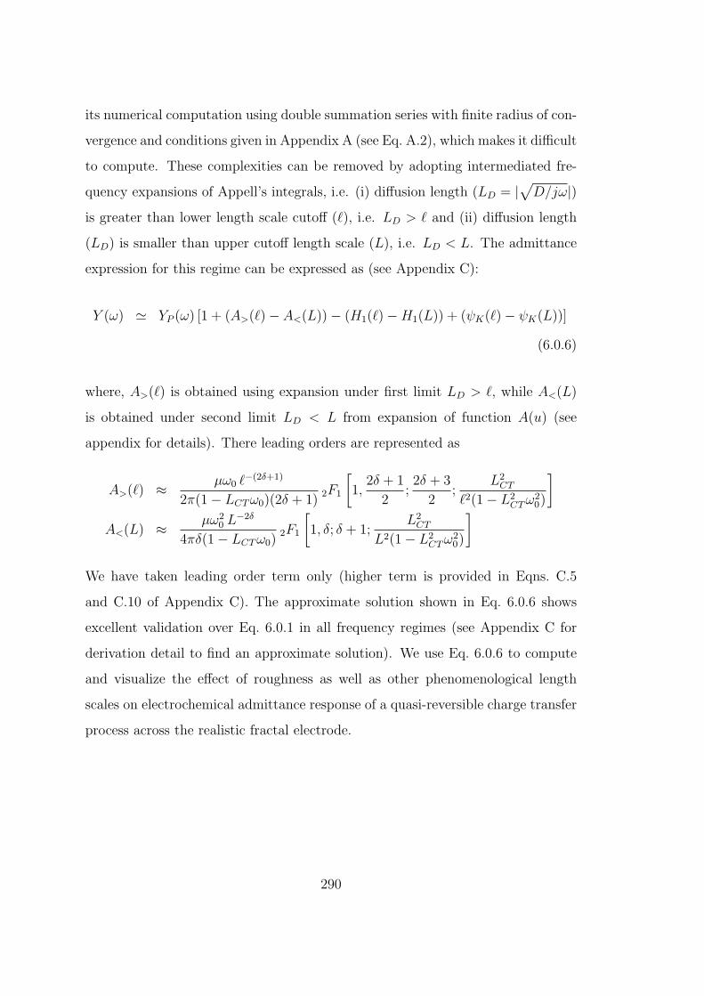
its numerical computation using double summation series with finite radius of con-

vergence and conditions given in Appendix A (see Eq. A.2), which makes it difficult

to compute. These complexities can be removed by adopting intermediated fre-

quency expansions of Appell’s integrals, i.e. (i) diffusion length (LD = |√D/jω|)

is greater than lower length scale cutoff (ℓ), i.e. LD > ℓ and (ii) diffusion length

(LD) is smaller than upper cutoff length scale (L), i.e. LD < L. The admittance

expression for this regime can be expressed as (see Appendix C):

Y (ω) ≃ YP (ω) [1 + (A>(ℓ)− A<(L))− (H1(ℓ)−H1(L)) + (ψK(ℓ)− ψK(L))]

(6.0.6)

where, A>(ℓ) is obtained using expansion under first limit LD > ℓ, while A<(L)

is obtained under second limit LD < L from expansion of function A(u) (see

appendix for details). There leading orders are represented as

A>(ℓ) ≈ µω0 ℓ−(2δ+1)

2π(1− LCTω0)(2δ + 1)2F1

[1,

2δ + 1

2;2δ + 3

2;

L2CT

ℓ2(1− L2CTω

20)

]A<(L) ≈ µω2

0 L−2δ

4πδ(1− LCTω0)2F1

[1, δ; δ + 1;

L2CT

L2(1− L2CTω

20)

]

We have taken leading order term only (higher term is provided in Eqns. C.5

and C.10 of Appendix C). The approximate solution shown in Eq. 6.0.6 shows

excellent validation over Eq. 6.0.1 in all frequency regimes (see Appendix C for

derivation detail to find an approximate solution). We use Eq. 6.0.6 to compute

and visualize the effect of roughness as well as other phenomenological length

scales on electrochemical admittance response of a quasi-reversible charge transfer

process across the realistic fractal electrode.

290

7 Results and Discussions

In this section we present results obtained for the theoretical model for Randles-

Ershler admittance under supported conditions for rough electrode describe by

Eq. 6.0.1. To understand the double layer charging, charge transfer rates on

the impedance response at rough electrodes, we consider the various situations

with respect to different parameters involved. The resulting response will help

understand various regimes and the role of roughness in distinguishing the kinetics

of reactions.

Figures 8.2(a), (b) and (c) shows the plots of the log of impedance vs frequency,

phase vs log of frequency and Nyquist plot of rough electrode. The dotted lines,

black, blue and red represent the pure Warburg impedance, anomalous Warburg

(rough) impedance and Quasi-reversible (rough) impedance respectively. The solid

blue and black lines represent the planar and rough electric double layer impedance

given by Eq. 3.0.3 and Eq. 6.0.1 respectively.

Figures 8.2 (a) shows the log-log plot of Randles impedance in comparison to

various impedance limits: (1) pure Warburg (black dotted line), (2) anomalous

Warburg (blue dotted line) and (3) quasi-reversible cases (red dotted lines). One

can clearly see the difference in electrochemical response of Randles impedance

from the pure and anomalous Warburg impedances. The solid blue and black

lines corresponds to pure flat and rough Randles impedance. There is no differ-

ence in the response of rough and flat Randles impedance at very low and very

high response. Difference in impedance response is seen in intermediate frequen-

cies. At low frequencies we see all the plots merges. At intermediate frequencies

the Randles impedance differ from the pure Warburg, amomalous Warburg and

quasi-reversible impedance of rough electrode as it include the capacitive compo-

nent. The whole electrochemical response is divided into three regimes by two

characteristic time: τd and τc. The three distinctive regimes are : (1) Warburg

controlled (2) charge transfer controlled and (3) capacitive controlled.

291

Figures 8.2 (b) shows the phase vs log of frequency plot of Randles impedance.

The dotted black lines represent the classical pure Warburg phase. The blue dotted

line represents the anomalous Warburg in presence of roughness. The red dotted

lines represents the phase of a rough electrode undergoing quasi-reversible charge

transfer reaction. The solid blue and black lines represents phase of the planar

and rough in Randles situation. The rough Randles phase vs log frequency plots

clearly show four frequencies regimes: (1) in low frequencies, we see the diffusion

controlled pure classical Warburg regime where Φ(ω) = 45, (2) in intermediate,

we see anomalous Warburg where Φ(ω) > 45, (3) in high frequencies, we see

the charge transfer resistance controlled regimes where 0 < Φ(ω) < 45 and (4)

at very high frequencies, we see the double layer controlled regimes where 0 <

Φ(ω) < 90. The plots shows that phase behavior of planar and rough Randles

are very much different in intermediate and high frequencies. At intermediate

the phase angle of planar is much smaller than phase angle of rough and in high

frequencies the phase angle of planar is larger than the phase of rough electrode.

A clear difference is seen between the responses of planar and rough Randles phase

plot. While in the low frequencies the phase of planar Randles is lower than 45

(classical Warburg phase) the rough Randles show phase angle greater than 45

and at high frequencies. Both show same phase behavior at low and very high

frequencies. A clear difference in the phase behavior between the quasi-reversible

and Randles condition is also seen in high frequencies. At high frequencies the

phase angle goes to zero for quasi-reversible case whereas for Randles case the

phase is greater than zero and phase approach 90 as the frequency is increase.

The switchover from charge transfer resistance controlled to double layer capacitive

controlled is seen as change in value of phase angle.

Figure 8.2 (c) shows the Nyquist plot for the Randles impedance for a rough

electrode. Here one can see the difference from both the pure Warburg (black dot-

ted line), anomalous Warburg (blue dotted line) and the quasi-reversible impedance

(red dotted line). The blue solid line represent the pure flat electrode Randles

292

HaL

-2 0 2 4 60

1

2

3

logHwês-1L

logH»Z»êW

cm2 L

HbL

-2 0 2 4 60

20

40

60

80

logHwês-1L

FHw

êdeg

reeL

HcL

0 10 20 30 40 500

10

20

30

40

50

Z'HwLêW cm2

-Z

''HwLêW

cm2

Figure 8.2: (a) log-log plot of magnitude of impedance vs frequency. (b) phasevs log of frequency. (c) Nyquist plot- real component of impedance vs imaginarycomponent impedance as a function of frequency. These plots were generatedusing ℓ = 10 nm, DH = 2.23, L = 10 µm, µ = 2× 10−7(a.u), Rct = 40 Ω, Cd = 10µF/cm2, A0 = 1 cm2, diffusion coefficient (D = 5 ×10−6 cm2/s) and concentration(CO = CR = 5 mM) are used in our calculations.

293

impedance. The black solid line is the response of Randles impedance for a rough

electrode. The plots show two distinctive regimes- diffusion controlled regime and

the charge transfer controlled regimes. The size of usual semi-circle of the pure

Randles impedance is reduced in presence of roughness. Similar observation are

also reported in literature[80]. The diffusive arm of the Randles impedance ex-

actly corresponds to the quasi-reversible impedance of rough electrode. The slope

of impedance in diffusion controlled regimes for anomalous Warburg and rough

Randle is very much different from pure Warburg and greater than 45 indicating

the influence of roughness. Thus roughness have two major effect on the Nyquist

plot of Randles impedance- first the size of semi-circle is reduce in presence of

roughness and secondly it affects the slope of diffusion controlled impedance arm.

In presence of roughness the effective resistance sensed by the system is reduced

and this results in faster switchover from kinetic controlled to mass transfer con-

trolled as we lower the frequency. Due to lowering in the effective resistance of

the system the characteristic frequency τf = 1/CdRct value is shifted to higher

frequency. At high frequency the plots of pure Warburg, anomalous Warburg,

pure Randles and rough Randles merges.

Figure 8.3 (a) shows the effect of charge transfer resistance Rct on the log-

log plot of Randles impedance vs frequencies for a rough electrode. The pure

Warburg (black dotted line), anomalous Warburg (blue dotted line) and quasi-

reversible (red dotted lines) impedances are also shown for comparison. Here we

find that effect of charge transfer on the Randles impedance of rough electrode is

seen in the intermediate frequencies. At low frequencies the Randles impedance

response merges with the classical and anomalous Warburg and quasi-reversible

impedances. A major difference in the responses is seen in the high frequencies.

The effect of of charge transfer resistance on the Randles impedance is seen in

the intermediate frequencies. The plateau region in the impedance response cor-

responds to the charge transfer controlled regime which is also evident with the

quasi-reversible response plot. Increasing the charge transfer resistance gradually

294

lifts the plateau region in the impedance plot. No effect of charge transfer re-

sistance is seen in the low frequency region and the responses merges with the

classical Warburg response. Similarly no effect of charge transfer resistance is

seen in the high frequency region as it correspond to purely capacitive controlled

regime.

Figure 8.3 (b) shows the effect of charge transfer resistance on phase vs log

of frequency of Randles impedance of rough electrode. The pure Warburg (black

dotted line), anomalous Warburg (blue dotted line) and quasi-reversible (red dot-

ted lines) impedances are also shown for comparison. In the intermediate and

low frequency the increase in charge transfer lower the value of phase but at high

frequencies the increase in charge transfer resistance increases the value of phase.

Figure 8.3 (c) shows the effect of charge transfer resistance on the Nyquist plot

of the Randles impedance for a rough electrode. As we increase the value of charge

transfer resistance the size of semi-circle is increase and value of the characteristic

timeτf shifts to lower frequencies. This means that the system becomes more

more and more kinetic controlled as we increase the charge transfer resistance.

The slope of impedance arm in all Randles impedance plots are same in the mass-

transfer controlled low frequency regime but the value of slope is greater than the

pure Warburg impedance, indicating the influence of roughness.

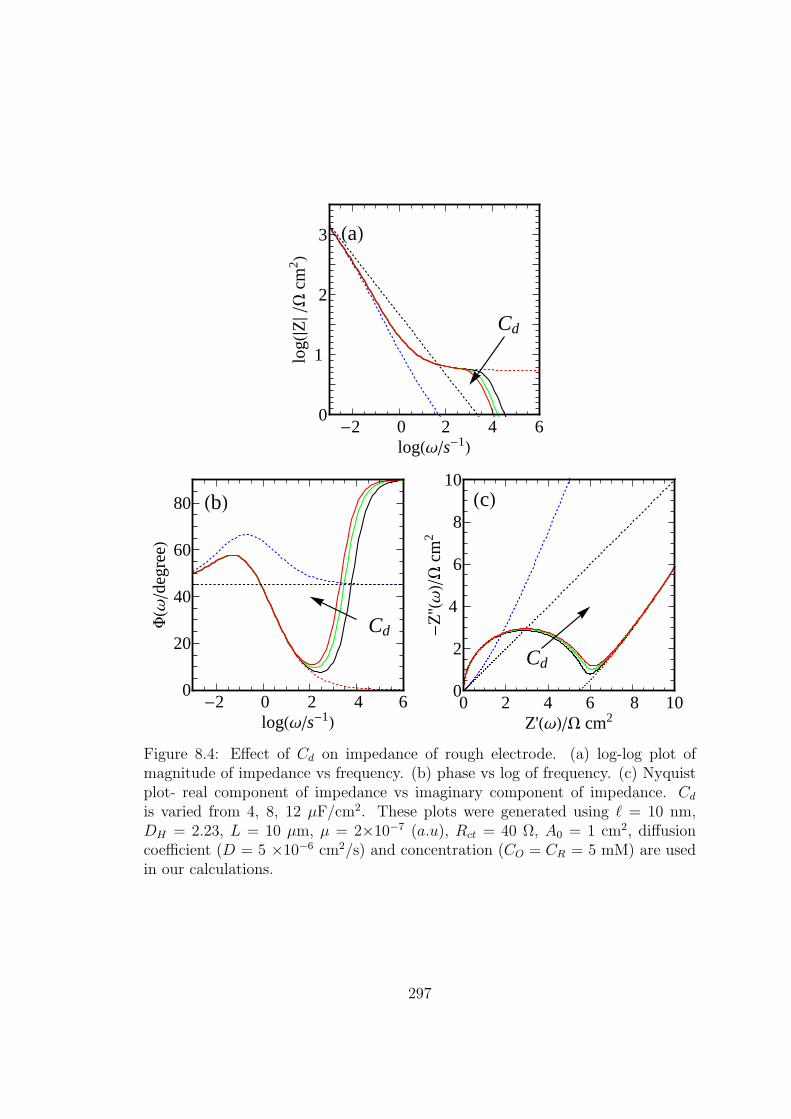
Figure 8.4 (a) shows the effect of double layer capacitance on the log-log plot

of Randles impedance vs frequency. Here we see that as we increase the value

of double layer capacitance the switchover from charge transfer controlled to ca-

pacitive controlled becomes faster and faster and the the characteristic crossover

frequency progressively shifts to lower frequencies. Now effect is seen in the low

frequencies and the impedance response mergers with the pure Warburg limit.

Figure 8.4 (b) shows the effect of double layer capacitance on the phase vs log

of frequency. Increasing the value of double layer capacitance.

Figure 8.4 (c) shows the effect of double layer capacitance on the Nyquist

plot. Increasing the capacitance, the kinetic control regime is extended at lower

295

Rct

HaL

-2 0 2 4 60

1

2

3

logHwês-1L

logH»Z»êW

cm2 L

HbL

Rct

-2 0 2 4 60

20

40

60

80

logHwês-1L

FHw

êdeg

reeL

HcL

Rct

0 5 10 150

5

10

15

Z'HwLêW cm2

-Z

''HwLêW

cm2

Figure 8.3: Effect of Rct on impedance of rough electrode. (a) log-log plot ofmagnitude of impedance vs frequency. (b) phase vs log of frequency. (c) Nyquistplot- real component of impedance vs imaginary component of impedance. Rct

is varied from 40, 50, 60, 70 Ω. These plots were generated using ℓ = 10 nm,DH = 2.23, L = 10 µm, µ = 2×10−7 (a.u), Cd = 10 µ F/cm2, A0 = 1 cm2,diffusion coefficient (D = 5× 10−6 cm2/s) and concentration (CO = CR = 5 mM)are used in our calculations.

296

Cd

HaL

-2 0 2 4 60

1

2

3

logHwês-1L

logH»Z»êW

cm2 L

HbL

Cd

-2 0 2 4 60

20

40

60

80

logHwês-1L

FHw

êdeg

reeL

HcL

Cd

0 2 4 6 8 100

2

4

6

8

10

Z'HwLêW cm2

-Z

''HwLêW

cm2

Figure 8.4: Effect of Cd on impedance of rough electrode. (a) log-log plot ofmagnitude of impedance vs frequency. (b) phase vs log of frequency. (c) Nyquistplot- real component of impedance vs imaginary component of impedance. Cd

is varied from 4, 8, 12 µF/cm2. These plots were generated using ℓ = 10 nm,DH = 2.23, L = 10 µm, µ = 2×10−7 (a.u), Rct = 40 Ω, A0 = 1 cm2, diffusioncoefficient (D = 5 ×10−6 cm2/s) and concentration (CO = CR = 5 mM) are usedin our calculations.

297

frequencies. This is seen in the plots as increasing the size in the semicircle. The

mixed region is mostly affected.

In order to understand the effect of roughness on the electrochemical response

we plot various impedance response varying the fractal morphological parameters:

fractal dimensions (DH), lower cutoff length, (l), and width of the interface, (µ).

The effect of roughness is also seen in the Nyquist plot in three different regimes:

(1) kinetic controlled, (2) mass transfered controlled and (3) mixed controlled is

clearly seen. In the plots the semicircle represents the kinetic controlled regime

and the raising arm represents the mass transfer controlled regime. The dip valley

region in between the semicircle and raising arm represent the mixed controlled

regime.

Figure 8.5 (a) is a Nyquist plot showing the effect of fractal dimension DH on

the Randles impedance. The black line corresponds to the pure Randles case with

no roughness. Increasing the fractal dimension, increases the slope of impedance

plot in the mass transfer regime. This clearly show that the fractal nature of

electrode has a strong influence on the mass transport. The inset in fig 8.5 (a)

shows the enlarged Nyquist plot in high frequency regime. The increase in fractal

dimension not only decrease the size of semicircle but also increases the charac-

teristic frequency at which the system switchover from mass transfer to kinetic

controlled. The decrease in size of semicircle indicates the reduction in the effec-

tive charge transfer resistance. This means on rough electrode the charge transfer

is enhanced. In other words increasing fractal dimension makes the system more

charge transfer controlled.

Figure 8.5 (b) shows the effect of lowest length scale of fractality on the Ran-

dles impedance. The black line corresponds to the pure Randles impedance for

a flat electrode. The increase in lower length cutoff decreases the slope of the

mass transfer impedance arm. Increasing the lowest length of fractality, the slope

of impedance in the mass transfer controlled regime is gradually reduced and

approach the classical Warburg phase value of 45. The inset in figure 8.5 (b)

298

DH

HaL

0 200 400 600 800 10000

200

400

600

800

1000

Z'HwLêW cm2

-Z

''HwLêW

cm2

0 10 200

10

20

HbL

0 200 400 600 800 10000

200

400

600

800

1000

Z'HwLêW cm2

-Z

''HwLêW

cm2

0 5 100

5

10

m

HcL

0 200 400 600 800 10000

200

400

600

800

1000

Z'HwLêW cm2

-Z

''HwLêW

cm2

0 10 200

10

20

Figure 8.5: Nyquist plot showing the effect of roughness impedance of roughelectrode. (a) Effect of fractal dimension (DH). DH is varied from 2.1, 2.15, 2.2,2.25. (b) Effect of lowest scale of fractality (ℓ). ℓ(nm) is varied from 5, 10, 15, 20.(c) Effect of width of interface (µ). µ(10−7) is varied from 0.5, 1, 2, 4 (a.u). Theseplots were generated using Rct = 40 Ω, Cd = 10 µ F/cm2, A0 = 1 cm2, diffusioncoefficient (D = 5× 10−6 cm2/s) and concentration (CO = CR = 5 mM) are usedin our calculations.

299

shows the enlarged Nyquist plot in high frequency regime. In the high frequen-

cies, increasing the lower length scale, the size of the semicircle increases which

indicates that the effective charge transfer resistance is increased. Thus decreasing

the roughness of the electrode by increasing the lower cutoff length, the effective

charge transfer resistance is increase and the system becomes more and more ki-

netic controlled.

Figure 8.5 (c) shows the effect of strength of fractality on the Randles impedance.

In this case the black line corresponds to the response of planar Randles impedance.

Increasing the strength of fractality (µ), the slope of the impedance in the mass

controlled regime increased. The inset in figure 8.5 (c) shows the influence of

strength of fractality on the high frequency. Increasing the strength of fractal-

ity increases the slope in the mass controlled regime and the size of semicircle is

reduced.

8 Conclusions

An ab initio theory for impedance finite charge transfer under diffusion limited

(quasi reversible ) in presence of double layer charging a rough electrode at Randles-

Ershler level is developed under supported conditions where ohmic (iRΩ) is negli-

gible. Various limiting impedances, pure Warburg, anomalous Warburg and quasi-

reversible impedances are obtained as special cases of Randles-Ershler impedance

under limiting conditions. Three phenomenological regimes: (1) kinetic controlled

(Faradiac) (2) mass transfer (diffusion) controlled and (3) mixed are clearly identi-

fied. The corresponding two time scales, τc and τd are identified. The electrochem-

ical response is found to depend on two length scales- diffusion length (D/ω)1/2

and charge transfer layer thickness Lct. The theory unravels the the influence of

roughness under kinetic controlled, mixed and mass transfer controlled situation

governed by the two characteristic phenomenological length scales. A detailed

analysis of the effect of roughness on Randles impedance is carried out. The re-

300

sponse of Randles impedance for a rough electrode is found to be different from

the planar classical Randles equivalent circuit model. The Randles impedance re-

sponse of a fractal electrode is found to be affected by the morphological features

characterizing the fractal viz., fractal dimension DH , surface roughness amplitude

µ, and the smallest length scale of fractality ℓ. The following conclusions are

drawn for Randles impedance with fractal roughness from the model developed:

1. The Randles-Ershler impedance and phase responses shows four regimes : (1)

low frequency region showing classical Warburg impedance with phase angle

Φ(ω) = 45, (2) anomalous Warburg for intermediate frequencies where

phase angle Φ(ω) > 45, (3) quasi-reversible charge transfer controlled where

the phase angle is 0 < Φ(ω) < 45 and (4) purely capacitive controlled with

phase angle Φ(ω) = 90.

2. The Nyquist plot indicate that the kinetic controlled (Faradaic) regime and

the mass transfer (diffusion ) controlled regime is affected by the roughness

of electrode. The size of the semicircle (kinetic controlled regime) is found

to be affected by value charge transfer resistance, double layer capacitance

and the roughness of electrode. As the roughness increases the Nyquist plot

shows smaller circles. Our results shows that the effective resistance decrease

as the roughness of electrode increases. Similar results are also reported in

literature [80]. This also not only affects the electric double layer charging

time τc but also the switch-over time τD

3. The slope of impedance in the mass transfer region is strongly affected by

the fractal dimension. While increasing the fractal dimension DH and width

of interface, the slope is greater than 45 resulting in anomalous Warburg

behavior. Fractal dimension also affects the kinetic controlled regimes. In-

creasing the fractal dimension and width of interface the size of the semi-

circle is reduced with simultaneous change in the characteristic switchover

time of the system.

301

4. In the mass transfer regimes the deviation from the pure Warburg impedance

arise in the frequency range L2CT/D ≤ ω ≤ (L2

CT + h2)/D.

5. The model developed here provide a way to estimate effective charge transfer

resistance in presence of electric double layer for a rough electrode.

Finally in conclusion we say taking into account the roughness in presence of

double layer charging leads to a very different Randles-Eshler impedance unlike

the classical Randles-Ershler equivalent circuit model. A general impression that

CPE behavior is sufficient to modeling of roughness in electrical circuit may be

inadequate as the theory developed have shown that the roughness do affect both

the kinetic controlled regime and mass transfer controlled regimes. We also have

shown how effect of roughness can be seen in kinetic controlled regime without

without any CPE element. An important word of caution is that the geometry

of the electrode and the electrochemical process involving at the electrode are

not independent and hence proper consideration must be made while interpreting

EIS data. The promising aspect of the Randles-Ershler impedance developed here

perhaps may be wide varied applications in understanding a number of electro-

chemical process occurring in batteries, fuel cells, pseudocapacitors etc. A theory

for generalized Randles-Ershler impedance on rough electrode for unsupported

condition including ohmic correction, electric double layer roughness effect will be

present elsewhere.

302

Appendices

A Useful Integrals and Expansions

For solving and attaining the analytical solution shown in Eq. 6.0.1, for the prob-

lem of quasi-reversible charge transport (finite charge partial diffusion limited)

processes, we have to solve an integral shown in Eq. 3.0.2 and need to have been

following formulae:

F1[a; b1, b2; c; z1, z2] =Γ(c)

Γ(a)Γ(c− a)

∫ 1

0

ma−1(1−m)c−a−1

(1−mz1)b1(1−mz2)b2dm

(A.1)

series representation of Appell double hypergeometric function (F1[.]) is:

F1[a; b1, b2; c; z1, z2] =∞∑

m1=0

∞∑m2=0

(a)m1+m2(b1)m1(b2)m2

(c)m1+m2 m1!m2!zm11 zm2

2

; [|z1| < 1, |z2| < 1] (A.2)

Integral definition of Gauss hypergeometric function (2F1[.]) is:

2F1[a, b; c; z] =Γ(c)

Γ(b)Γ(c− b)

∫ 1

0

mb−1(1−m)c−b−1

(1−mz)adm (A.3)

special cases of Appell hypergeometric function (F1[.]) and Gauss hypergeometric

function (2F1[.]) are:

F1[a; b1, b2; c; z, 0] = 2F1[a, b; c; z] (A.4)

2F1[a, b; c; 0] = 1 (A.5)

at RCT → 0, situation which gives Warburg admittance as a special case of quasi-

reversible charge transfer admittance. These expansions are useful in explaining

the influence of heterogeneous kinetics.

303

B Derivation to Integral for Finite Fractal Rough-

ness

Substitution of the power spectrum shown in Eq. 5.0.1 into Eq. 3.0.2, give rise to

integral expression, which is further split into two limits can be expressed as:

ω0

2π

∫ 1/ℓ

1/L

µK2DH−6∥ (ω∥ − ω0)

1 + ω∥LCT

dK∥ =ω0

2π

∫ 1/ℓ

0

µK2DH−6∥ (ω∥ − ω0)

1 + ω∥LCT

dK∥ −

ω0

2π

∫ 1/L

0

µK2DH−6∥ (ω∥ − ω0)

1 + ω∥LCT

dK∥

(B.1)

where, ω∥ =√ω20 +K2

∥ and ω0 =√jω/D. To solve the above integral, we take

first part of Eq. B.1. Second part of Eq. B.1 can be similarly calculated, then we

have

ω0

2π

∫ 1/ℓ

0

µK2DH−6∥ (ω∥ − ω0)

1 + ω∥LCT

dK∥ =ω0

2π

∫ 1/ℓ

0

µK2DH−6∥ (ω∥ − ω0)(1− ω∥LCT )

1− ω2∥L

2CT

dK∥

(B.2)

Eq. B.2 can be further generalized to make the integral solvable and can be given

as

ω0

2π

∫ 1/ℓ

0

µK2DH−6∥ (ω∥ − ω0 − ω2

∥LCT + ω0ω∥LCT )

1− ω2∥L

2CT

dK∥ (B.3)

simplifying Eq. B.3, we have

ω0

2π

∫ 1/ℓ

0

µK2DH−6∥ (ω∥ + ω0ω∥LCT − ω0 − ω2

0LCT )

1− ω2∥L

2CT

dK∥

−ω0

2π

∫ 1/ℓ

0

µK2DH−4∥ LCT

1− ω2∥L

2CT

dK∥ (B.4)

304

Complete integral expression after substitution of Eq. 5.0.1 in Eq. 3.0.2, can be

expressed as

ψDK(ℓ) =µω0(1 + ω0 LCT )

2π

∫ 1/ℓ

0

dK∥K2DH−6

∥ (ω∥ − ω0)

(1− ω2∥ L

2CT )

(B.5)

ψK(ℓ) =µω0 LCT

2π

∫ 1/ℓ

0

dK∥K2DH−4

∥

2(1 + ω0 LCT )−∫ 1/ℓ

0

dK∥K2DH−4

∥

(1− ω2∥ L

2CT )

(B.6)

substitute y = K∥ℓ and ω∥ =√ω20 +K2

∥ in Eq. B.5, we have

µω0(1 + LCTω0)

2πℓ5−2DH

∫ 1

0

y2DH−6√

(ω20 + y2/ℓ2)(

(1− ω20L

2CT )−

y2L2CT

ℓ2

)dy−∫ 1

0

ω0y2DH−6(

(1− ω20L

2CT )−

y2L2CT

ℓ2

)dy (B.7)

solution of first part of Eq. B.7 can be obtained by using following steps

µω0(1 + LCTω0)

2πℓ5−2DH

∫ 1

0

y2DH−6√

(ω20 + y2/ℓ2)(

(1− ω20L

2CT )−

y2L2CT

ℓ2

)dyput y2 = m and rearranging the term, above integral becomes

µω0(1 + LCTω0)

4πℓ5−2DH

∫ 1

0

mDH−7/2(ω20 +m/ℓ2)

1/2

((1− ω20L

2CT )−

mL2CT

ℓ2)dm (B.8)

taking common out some terms to make the above integral simple which can be

map into the integral of Appell function shown in Eq. A.1

µω0(1 + LCTω0)ℓ5−2DH

4π

ω0

(1− ω20L

2CT )

∫ 1

0

mDH−7/2(1 +m/ω20ℓ

2)1/2

(1−m)0

(1− mL2CT

(1−ω20L

2CT )ℓ2

)dm

305

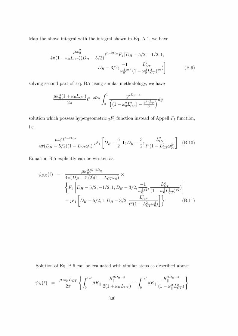
Map the above integral with the integral shown in Eq. A.1, we have

µω20

4π(1− ω0LCT )(DH − 5/2)ℓ5−2DHF1 [DH − 5/2;−1/2, 1;

DH − 3/2;−1

ω20ℓ

2,

L2CT

(1− ω20L

2CT )ℓ

2)

](B.9)

solving second part of Eq. B.7 using similar methodology, we have

µω20(1 + ω0LCT )

2πℓ5−2DH

∫ 1

0

y2DH−6((1− ω2

0L2CT )−

y2L2CT

ℓ2

)dysolution which possess hypergeometric 2F1 function instead of Appell F1 function,

i.e.

µω20ℓ

5−2DH

4π(DH − 5/2)(1− LCTω0)2F1

[DH − 5

2, 1;DH − 3

2;

L2CT

ℓ2(1− L2CTω

20)

](B.10)

Equation B.5 explicitly can be written as

ψDK(ℓ) =µω2

0ℓ5−2DH

4π(DH − 5/2)(1− LCTω0)×

F1

[DH − 5/2;−1/2, 1;DH − 3/2;

−1

ω20ℓ

2,

L2CT

(1− ω20L

2CT )ℓ

2)

]− 2F1

[DH − 5/2, 1;DH − 3/2;

L2CT

ℓ2(1− L2CTω

20)

](B.11)

Solution of Eq. B.6 can be evaluated with similar steps as described above

ψK(ℓ) =µω0 LCT

2π

∫ 1/ℓ

0

dK∥K2DH−4

∥

2(1 + ω0 LCT )−∫ 1/ℓ

0

dK∥K2DH−4

∥

(1− ω2∥ L

2CT )

306

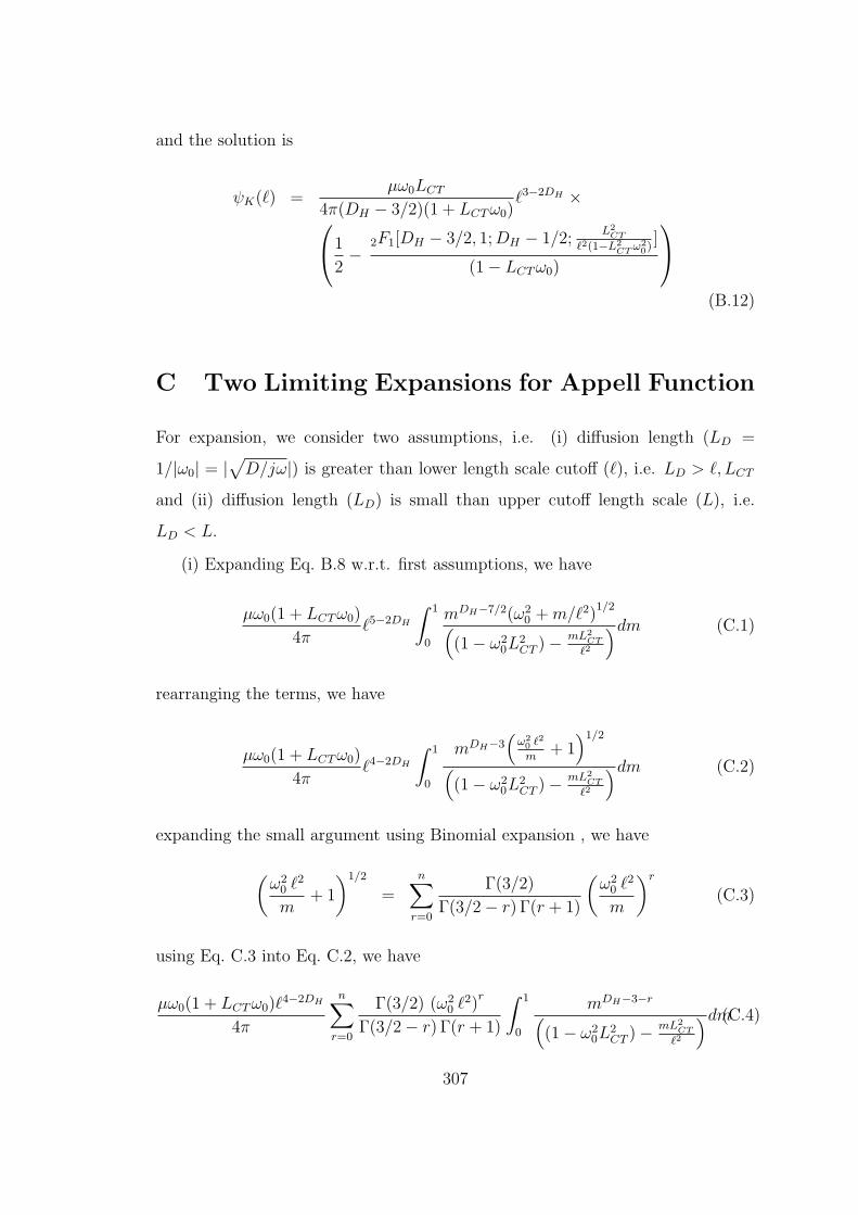
and the solution is

ψK(ℓ) =µω0LCT

4π(DH − 3/2)(1 + LCTω0)ℓ3−2DH ×1

2−

2F1[DH − 3/2, 1;DH − 1/2;L2CT

ℓ2(1−L2CTω2

0)]

(1− LCTω0)

(B.12)

C Two Limiting Expansions for Appell Function

For expansion, we consider two assumptions, i.e. (i) diffusion length (LD =

1/|ω0| = |√D/jω|) is greater than lower length scale cutoff (ℓ), i.e. LD > ℓ, LCT

and (ii) diffusion length (LD) is small than upper cutoff length scale (L), i.e.

LD < L.

(i) Expanding Eq. B.8 w.r.t. first assumptions, we have

µω0(1 + LCTω0)

4πℓ5−2DH

∫ 1

0

mDH−7/2(ω20 +m/ℓ2)

1/2((1− ω2

0L2CT )−

mL2CT

ℓ2

)dm (C.1)

rearranging the terms, we have

µω0(1 + LCTω0)

4πℓ4−2DH

∫ 1

0

mDH−3(

ω20 ℓ2

m+ 1)1/2(

(1− ω20L

2CT )−

mL2CT

ℓ2

)dm (C.2)

expanding the small argument using Binomial expansion , we have

(ω20 ℓ

2

m+ 1

)1/2

=n∑

r=0

Γ(3/2)

Γ(3/2− r) Γ(r + 1)

(ω20 ℓ

2

m

)r

(C.3)

using Eq. C.3 into Eq. C.2, we have

µω0(1 + LCTω0)ℓ4−2DH

4π

n∑r=0

Γ(3/2) (ω20 ℓ

2)r

Γ(3/2− r) Γ(r + 1)

∫ 1

0

mDH−3−r((1− ω2

0L2CT )−

mL2CT

ℓ2

)dm(C.4)307

rearranging and solving the integral using method shown in Appendix (B), we

have

µω0

4π(1− LCTω0)ℓ4−2DH

n∑r=0

Γ(3/2)

Γ(3/2− r) Γ(r + 1)

(ω20 ℓ

2)r 1

(DH − 2− r)

2F1

[1, DH − 2− r;DH − 1− r;

L2CT

ℓ2(1− L2CTω

20)

](C.5)

(ii) Expanding Eq. B.8 w.r.t. second assumptions, we have

µω0(1 + LCTω0)

4πL5−2DH

∫ 1

0

mDH−7/2(ω20 +m/L2)

1/2((1− ω2

0L2CT )−

mL2CT

L2

) dm (C.6)

rearranging the term in such a way that we can use second assumption, therefore

µω20(1 + LCTω0)

4πL5−2DH

∫ 1

0

mDH−7/2(1 + m

ω20 L2

)1/2((1− ω2

0L2CT )−

mL2CT

L2

)dm (C.7)

expanding the small argument with Binomial expansion, we have

(1 +

m

ω20 L

2

)1/2

=n∑

r=0

Γ(3/2)

Γ(3/2− r) Γ(r + 1)

(m

ω20 L

2

)r

(C.8)

substituting Eq. C.8 into Eq. C.7, we have

µω20(1 + LCTω0)L

5−2DH

4π×

n∑r=0

Γ(3/2)

Γ(3/2− r) Γ(r + 1)(ω20 L

2)r

∫ 1

0

mDH−7/2+r((1− ω2

0L2CT )−

mL2CT

L2

)dm (C.9)

308

solving the integral using method shown in Appendix (B), we have

µω20

4π(1− LCTω0)L5−2DH

n∑r=0

Γ(3/2)

Γ(3/2− r) Γ(r + 1)

(1

ω20 L

2

)r1

(DH − 52+ r)

2F1

[1, DH − 5

2+ r;DH − 3

2+ r;

L2CT

L2(1− L2CTω

20)

](C.10)

309

Bibliography

[1] G. T. Teixidor, B.Y. Park, P. P. Mukherjee, Q. Kang, M.J. Madou, Elec-

trochim. Acta 54 (2009) 5928.

[2] M. Park, X. Zhang, M. Chung, G. B. Less, A. M. Sastry, J. Power Sources

195 (2010) 7904.

[3] P. M. Biesheuvel, A. A. Franco, M. Z. Bazant, J. Electrochem. Soc. 156 (2)

(2009) B225.

[4] R. Ahmed, K. Reifsnider, Int. J. Electrochem. Sci. 6 (2011) 1159.

[5] T. Amemiya, K. Hashimoto, A. Fujishima, J. Phys. Chem. 97 (1993) 9736.

[6] V. V. Nikonenko, A. E. Kozmai, Electrochim. Acta 56 (2011) 1262.

[7] A. Hauch, A. Georg, Electrochim. Acta 46 (2001) 3457.

[8] P. M. Biesheuvel, Y. Fu, M. Z. Bazant, Phys. Rev. E 83 (2011) 061507.

[9] B. Sapoval, Phys. Rev. Lett. 73 (1994) 3314.

[10] V. V. Pototskaya, N.E. Evtushenko, O. I. Gichan, Russ. J. Electrochem. 37

(2001) 857.

[11] V. V. Pototskaya, N. E. Evtushenko, O. I. Gichan, Russ. J. Electrochem. 40

(2004) 424.

[12] M. Giona, M. Giustiniani, Sep. Technol. 6 (1996) 99.

310

[13] Z. Hens, W. P. Gomes, J. Phys. Chem. B 101 (1997) 5814.

[14] D. F. Franceschetti, J. R. Macdonald, J. Electrochem. Soc. 129 (1982) 1754.

[15] J.Y. Go, S. I. Pyun, J. Solid State Electrochem. 11 (2007) 323.

[16] A. L. Mehaute, G. Crepy, Solid State Ionics 9 (1983) 17.

[17] L. Nyikos, T. Pajkossy, Electrochim. Acta 31 (1986) 1347.

[18] Z. Kerner, T. Pajkossy, Electrochim. Acta 46 (2000) 207.

[19] A. Maritan, A. L. Stella, F. Toigo, Phys. Rev. B 40 (1989) 9269.

[20] S. Srivastav, R. Kant, J. Phys. Chem. C .10.1021/jp2024632

[21] R. Kumar, R. Kant, J. Phys. Chem. C 113 (2009) 19558.

[22] B. A. Boukamp, H. J. M. Bouwmeester, Solid State Ionics 157 (2003) 29.

[23] T. Pajkossy, A. Borosy, A. Imre, S. A. Martemyanov, G. Nagy, R. Schiller,

L. Nyikos, J. Electroanal. Chem. 366 (1994) 69.

[24] A. S. Levy, D. Avnir, J. Phys. Chem. 97 (1993) 10380.

[25] A. Chaudhari, C. C. S. Yan, S.L. Lee, Chem. Phys. Lett. 351 (2002) 341.

[26] M. O. Coppens, G. F. Froment, Chem. Eng. Sci. 50 (1995) 1013.

[27] P. G. de Gennes, C. R. Acad. Sci. (Paris) Ser, II 295 (1982) 1061.

[28] R. Kopelman, Science 241 (1988) 1620.

[29] M. Sahimi, M. McKarnin, T. Nordahl, et al. Phys. Rev. A 32 (1985) 590.

[30] D. B. Avraham, S. Havlin, Diffusion and Reactions in Fractals and Disordered

Systems (Cambridge University Press, New York, 2000).

[31] M. Rosvall, Electrochem. Commn. 2 (2000) 791.

311

[32] E. Barsoukov, J. R. Macdonald, Impedance Spectroscopy Theory, Experi-

ment, and Applications; Wiley-Interscience, Second Edition, 2005.

[33] K. J. Vetter, Electrochemical Kinetics, Theoretical and Experimental As-

pects, Academic Press Inc. (London) Ltd. 1967.

[34] S. K. Rangarajan, J. Electroanal. Chem. 25 (1970) 344.

[35] S. K. Rangarajan, J. Electroanal. Chem. (1974) 55, 297; 55, 329; 55, 337; 55,

363.

[36] P. Delahay, K. Holub, J. Electroanal. Chem. 16 (1968) 131.

[37] P. Delahay, G. G. Susbielles, J. Phys. Chem. 70 (1966) 1350.

[38] K. Holub, G. Tessari, P. Delahay, J. Phys. Chem. 71 (1967) 2612.

[39] R. L. Birke, J. Electroanal. Chem. 33 (1971) 201.

[40] D. M. Mohilner, J. Phys. Chem. 68 (1964) 623.

[41] M. L. Olmstead, R. S. Nicholson, J. Phys. Chem. 72 (1968) 1650.

[42] R. S. Rodgers, L. Meites, J. Electroanal. Chem. 16 (1968) 1.

[43] G. G. Susbielles, P. Delahay, J. Electroanal. Chem. 17 (1968) 289.

[44] Monera, H.; Levi, R. D.; J. Electroanal. Chem. 35 (1972), 103.

[45] D. E. Smith, Anal. Chem. 36 (1964) 962.

[46] J. E. B. Randles, Disc. Far. Soc. 1 (1947) 11.

[47] P. M. Biesheuvel, Y. Fu, M. Z. Bazant, Phys. Rev E 83 (2011) 061507.

[48] D. R. Franceschetti, J. R. Macdonald, R. P. Buck, J. Electrochem. Soc. 138

(1991) 1368.

[49] J. R. Macdonald, D. R. Franceschetti, J. Chem. Phys. 68 (1978) 1614.

312

[50] B. Sapoval, J. N. Chazalviel, J. Peyriere, Phys. Rev. A. 38 (1988) 5867.

[51] B. Sapoval, R. Gutfraind, P. Meakin, M. Keddam, H. Takenouti, Phys. Rev.

E 48 (1993) 3333.

[52] B. B. V. Ershler, Disc. Far. Soc. 1 (1947) 269.

[53] R. Kant, S. K. Rangarajan, J. Electroanal. Chem. 368 (1994) 1.

[54] R. Kant, S. K. Rangarajan, J. Electroanal. Chem. 396 (1995) 285.

[55] R. Kant, S. K. Rangarajan, J. Electroanal. Chem. 552 (2003) 141.

[56] R. de Levi, Annal. of Biomedical Eng. 20 (1992) 337.

[57] M. E. Orazem, B. Tribollet, Electrochemical Impedance Spectroscopy, A John

Wiley & Sons, Inc., Publication, 2008.

[58] J. Newman, J . Electrochem. Soc. 117 (1970) 198.

[59] T. Pajkossy, D. M. Kolb, Electrochim. Acta 53 (2008) 7403.

[60] M. H. Martin, A. Lasia, Electrochim. Acta 2011,

doi:10.1016/j.electacta.2011.02.068

[61] S. Chen, R. Pei, J. Am. Chem. Soc. 123 (2001) 10607.

[62] R. N. Vyas, K. Li, B. Wang, J. Phys. Chem. B 114 (2010) 15818.

[63] M.S. Rehbach, C. P. M. Bongenaar, A. G. Remijnse, J. H. Sluyters, Ind. J.

Tech. 24 (1986) 473.

[64] R. Kant, R. Kumar, V. K. Yadav, J. Phys. Chem. C 112 (2008) 4019.

[65] M. M. Islam, R. Kant, Electrochim. Acta 56 (2011) 4467.

[66] R. Kant, M. M. Islam, J. Phys. Chem. C 114 (2010) 19357.

[67] R. Kant, S. K. Rangarajan, J. Electroanal. Chem. 396 (1995) 285.

313

[68] S. K. Jha, R. Kant, J. Electroanal. Chem. 641 (2010) 78.

[69] R. Kumar, R. Kant, Electrochim. Acta 10.1016/j.electacta.2011.05.092.

[70] S. Srivastav, R. Kant, J. Phys. Chem. C. 115 (2011) 1232.

[71] B. M. Grafov, B. B. Damaskin, Electrochim. Acta 41 (1996) 2707.

[72] N. G. Bukun, A. E. Ukshe, Russ. J Electrochem. 45 (2009) 11.

[73] I. S. Atanasova, J. H. Durrellb, L. A. Vulkovaa, Z. H. Barberb, O. I. Yordanov,

Physica A 371 (2006) 361.

[74] R. J. Adler, The Geometry of Random Fields; John Wiley and Sons Ltd.,

New York, 1981.

[75] B. Mandelbrot, The Fractal Geometry of Nature (Freeman, San Francisco,

1982).

[76] J. Feder, Fractals; Plenum: New York, 1988.

[77] P. Pfeifer, D. Avnir, J. Chem. Phys. 79 (1983) 3558. D. Avnir, D. Farin, P.

Pfeifer, J. Chem. Phys. 79 (1983) 3566.

[78] W. N. Bailey, Appell’s Hypergeometric Functions of Two Variables: Gener-

alised Hypergeometric Series, Cambridge University Press, 1935.

[79] M. Abramowitz, I. A. Stegun, Handbook of Mathematical Functions, Dover

Publication inc., New York, 1972.

[80] G. Ruiz, C. J. Felice, Chaos, Solitons and Fractals 31 (2007) 327.

314