Chapter 8: Regression - Wright State Universitythaddeus.tarpey/stt630chap8.pdf · In the simple...

STT 430/630/ES 760 Lecture Notes: Chapter 8: Regression 1

March 5, 2009

Chapter 8: Regression

A very common problem in scientific studies is to determine how one variable depends on one or moreother variables. For example, is a hurricane’s wind speed related to the ocean water temperature? If so,what is the relationship?

Think back to the pelican egg example where data was collected on eggshell thickness and the level ofPCB’s in the birds. A question of interest is whether or not the eggshell thickness depends on the PCBlevel and if so, how does the PCB level affect eggshell thickness? Again, regression analysis can be usedto answer this question.

Francis Galton is credited with originating the term regression when he studied how heights of childrendepended on the heights of their parents. Can we predict a child’s height based on the height of thechild’s parents? Or, for parents of a particular height, what is the average height of their offspring? Linearregression is used to answer these types of questions.

Regression analysis is a broad field of statistics that deals with the problem of modelling how a variabledepends on one or more other variables. Consequently, regression analysis is one of the most heavily usedbranches of statistics. Regression models can become quite complicated. We begin this chapter with asimple model.

1 Simple Linear Regression

Figure 1 shows a scatterplot of the time to run two miles for a sample of middle-aged males versus themaximum volume of oxygen uptake in the blood (VO2 max). Clearly there appears to be a relation betweenhow fast one can run two miles and the maximum VO2 uptake. One of the goals of the current chapter isto learn how to model this type of data where one variable depends on another variable. From Figure 1, alinear relationship seems reasonable. The general term used to model how one variable depends on anothervariable is regression analysis.

In regression settings we have a response variable y (also known as the dependent variable) and a re-gressor variable x (also known as the independent or predictor variable). Data is collected on pairs(x1, y1), . . . , (xn, yn). The set up is that the average response depends on the value of x which defines aconditional expectation of y given x, denoted

E[y|x].

The way to think of this conditional expectation is: what is the average value of y for a given value of x?This conditional expectation is regarded as a function of x. In the simple linear regression, we model thisconditional expectation as a linear function:

E[y|x] = β0 + β1x. (1)

This is the equation of a line with y-intercept β0 and slope β1.

We can write (1) in another form:y = β0 + β1x + ε, (2)


40 45 50 55 60

600

700

800

900

1000

1100

1200

V02 Max vs. Time

Volume

Tim

e (s

econ

ds)

Figure 1: Scatterplot of time (to run 2 miles) versus Maximum volume of O2 uptake for a sample ofmiddle-aged men.


where ε is a random error which is needed because the points will not all lie exactly on a line.

In previous chapters, we have concentrated on estimating and testing hypotheses about the mean of apopulation. The mean is a parameter denoted by µ. In the regression setting, we also have parameters.In particular, the parameters are β0, the y-intercept, and the slope β1.

There is another parameter for the model (2), but it does not show up directly in the formula. That is,the random error is assumed to have a mean zero and a variance σ2. Thus, σ2, the error variance, is theother parameter of the model. For small values of σ2, the points in the scatterplot will be tightly clusteredabout the true regression line; for large values of σ2, the points will be spread out more from the regressionline.

In regression analysis, the common statistical problems of interest are:

• To test if the regressor variable x affects the response variable y.

• Predict a response for a given value of x.

• Estimate an average response for a given value of x.

• Model the relation between x and y.

2 Fitting Regression Lines: Least Squares

In Figure 1, the points show a roughly linear relation. If the simple linear regression model is the correctmodel, then there is a linear function defined in terms of β0 and β1 that models the relation. However, β0

and β1 are model parameters and are unknown. We must use the data to estimate the intercept and slopeof the line.

Question: How should we estimate the regression line?

Least-Squares. Looking back at Figure 1, the goal is to find a line that runs through the middle of thedata. There are several choices for “fitting” a line. The most common method of estimating the regressionline is to use least-squares. Let β0 and β1 denote the least-squares estimators of β0 and β1 respectively.Given a data point (xi, yi), the corresponding point on the least-squares regression line is yi = β0 + β1xi.The least-squares estimators are determined by minimizing (i.e. finding the least value) of the sum ofsquares:

n∑

i=1

(yi − yi)2 =

n∑

i=1

(yi − β0 − β1xi)2. (3)

Calculus can be used to solve this problem and the solution is given by the following equations:

β0 = y − β1x, (Least-Squares Estimator of the intercept) (4)

and

β1 =

∑ni=1 (xi − x)(yi − y)∑n

i=1 (xi − x)2, (Least-Squares Estimator of the slope) (5)

Given a set of data (x1, y1), . . . , (xn, yn), one can plug the data values into (4) and (5) to get the least-squares regression line.


40 45 50 55 60

600

700

800

900

1000

1100

1200

V02 Max vs. Time: Least−Squares Regression Line

Volume

Tim

e (s

econ

ds)

Figure 2: Scatterplot of time (to run 2 miles) versus Maximum volume of O2 uptake for a sample ofmiddle-aged men. The line is the least-squares regression line y = 1450.86− 12.86x.

Predicted Value. For a given data point (xi, yi), the predicted value or predicted response from theestimated regression line is denoted by yi and is given by

yi = β0 + β1xi. (6)

One reason for the popularity of the least-squares estimator is that if the error ε in (2) has a normaldistribution, then the least-squares estimators of the intercept and slope correspond to maximum likelihoodestimators.

Figure 2 shows the scatterplot of the V02 max data again along with the estimated least-squares regressionline that was computed using the above formulas. Using these formulas by hand is quite tedious. Typicallystatistical software such as SAS is used to do the computation (which we illustrate below) The least-squaresregression coefficients are found to be β0 = 1450.86 and β1 = −12.86. Therefore, the least-squares regressionline is given by the equation

y = 1450.86− 12.86x,

where x is the maximum VO2 uptake. Note that the estimated slope is negative indicating that as VO2 maxincreases, the time to run the two miles decreases. In particular, we estimate that for each additional unitof VO2 max, the time it takes to run the two miles decreases on average by 12.86 seconds. In Section 3.2we show how to compute a confidence interval for the slope coefficient.

Note that the intercept in the VO2 max example is estimated to be β0 = 1450.86. In the context ofthis example, the y-intercept is not interpretable. This value tells us where the regression line crosses they-axis. If the VO2 max value is x = 0, the predicted response is 1450.86. However, a value of zero for x is


not meaningful here since a value of x = 0 is not possible for a living middle aged man. Also, we do nothave data collected for values of x near zero. To predict a response near zero would require extrapolationwhich is always a very dangerous thing to do in statistics.

3 Inference for Regression Parameters

In simple linear regression there is only a single predictor variable x. Inference in simple linear regressionis usually focused on the slope β1 which relates how the response variable y depends on the predictor x.Recall that the slope tells us how much of a change one can expect to see in the response y for a unitchange in x. For instance, in the VO2 max example, how much faster would we expect a man to run 2miles if his VO2 max is increased by one unit? The slope answers this question. Thus, our interest is tonot only estimate the slope β1 but to obtain some measure of the reliability of the estimate.

In other examples, it may not be clear if there is a relation between x and y. For example, does exposureto lead in children lead to diminished IQ scores? Studies have been done that looked at IQ levels andblood lead levels in children. If lead does not affect IQ, then we would expect the slope of the regressionline relating IQ to lead levels to be zero (i.e. a horizontal line). Therefore, we have an interest in testinghypotheses about the slope of a regression line. We can also test hypotheses about the y-intercept of aline, but this is often not of interest.

Inference procedures for the slope are based on the following fact about the least-square estimator of theslope:

FACT 1: If (x1, y1), . . . , (xn, yn), is a random sample and the error term ε in (2) has a normal distribution,then the least square estimator of the slope β1 has a normal distribution with mean β1 and variance

σ2β1

=σ2

∑ni=1 (xi − x)2

.

That is, β1 has a normal distribution and is unbiased for the true regression slope β1. The least-squareestimator of the intercept β0 is also unbiased and follows a normal distribution. Even if the error ε is notexactly normal, the least-square estimators will still have approximately a normal distribution due to thecentral limit theorem effect, provided the sample size is sufficiently large.

Standard Error of the Estimated Slope. The square root of the variance of β1 is the standard errorof the estimated slope, denoted by SE(β1):

SE(β1) =

√√√√ σ2

∑ni=1 (xi − x)2

.

Of course σ2 is unknown and must be estimated. Therefore in practice we use the estimated standarderror for the slope:

SE(β1) =

√MSE∑n

i=1 (xi − x)2,

where MSE stands for mean squared error and is given by

MSE =n∑

i=1

(yi − (β0 + β1xi))2/(n− 2).


We will discuss MSE in greater detail below.

The next fact is used for statistical inference:

FACT 2: If (x1, y1), . . . , (xn, yn), is a random sample and the error term ε in (2) has a normal distribution,then

t =β1 − β1

SE(β1),

follows a t-distribution with n− 2 degrees of freedom.

Here are a couple important points:

• Note that the degrees of freedom for t is n−2, not n−1. The reason why is that we lose two degreesof freedom for estimating the intercept and slope of the line.

• The sampling distribution of t will have an approximate t distribution if the error ε deviates fromnormality, provided the deviation is not too severe or the sample size is large.

3.1 Hypothesis Testing for the Slope

A null hypothesis about the slope β1 of the regression line can be stated as

H0 : β1 = β10,

where β10 is some hypothetical value of the slope of interest. The alternative hypothesis can be one-sidedor two-sided: depending on the application:

Ha : β1 6= β10, or Ha : β1 > β10, or Ha : β1 < β10.

If β1 deviates substantially from the hypothesized value β10, then we would reject the null hypothesis. Thebenchmark for making this determination is the t-distribution based on Fact 2 above.

Test Statistic: t =β1 − β10

SE(β1). (7)

If H0 is true, then the t-test statistic follows a t-distribution on n− 2 degrees of freedom.

When performing a test about the slope at a significance level α, the following summarizes how hypothesistesting is done:

• If the alternative hypothesis is Ha : β1 6= β10, we reject H0 when t > tn−2,α/2 or t < −tn−2,α/2, wheret is the t-test statistic in (7).

• If the alternative hypothesis is Ha : β1 > β10, we reject H0 when t > tn−2,α.

• If the alternative hypothesis is Ha : β1 < β10 we reject H0 if t < −tn−2,α.


One of the most common tests in regression is to test if the slope differs from zero in which case thehypothesized value of the slope is β10 = 0 and the test statistic becomes

t =β1

SE(β1). (8)

In SAS (and many other statistical software packages), this test is done automatically when a regressionis run. The VO2 max example will be used to illustrate ideas:

/****************************************************************

One measure of cardiovascular fitness is the maximum volume of oxygen

uptake during exercise. 24 max. vol. of oxygen (column 1) was measured

on 24 middle aged men who ran 2 miles on a treadmill. Column 2 of the

data gives the time to run 2 miles in seconds.

(Reference: Ribisl and Kachadorian, "Maximal Oxygen Intake

Prediction in Young and Middle Aged Males," J. of Sports Medicine, 9,

1969, 17-22).

*********************************************************************/

data vo2;

input vol time;

datalines;

42.33 918

53.10 805

42.08 892

50.06 962

42.45 968

42.46 907

47.82 770

49.92 743

36.23 1045

49.66 810

41.49 927

46.17 813

48.18 858

43.21 860

51.81 760

53.28 747

53.29 743

47.18 803

56.91 683

47.80 844

48.65 755

53.69 700

60.62 748

56.73 775

;


run;

proc reg;

model time = vol;

run;

quit;

Here is the SAS output from PROC REG:

The REG Procedure

Model: MODEL1

Dependent Variable: time

Number of Observations Read 24

Number of Observations Used 24

Analysis of Variance

Sum of Mean

Source DF Squares Square F Value Pr > F

Model 1 129720 129720 42.01 <.0001

Error 22 67938 3088.10214

Corrected Total 23 197658

Root MSE 55.57070 R-Square 0.6563

Dependent Mean 826.50000 Adj R-Sq 0.6407

Coeff Var 6.72362

Parameter Estimates

Parameter Standard

Variable DF Estimate Error t Value Pr > |t|

Intercept 1 1450.86476 96.99988 14.96 <.0001

vol 1 -12.86113 1.98437 -6.48 <.0001

We will only discuss the last portion of this SAS output for now. The other portions of the output will beexplained in Section 6.

From the SAS output, we see that the least-squares regression line is given by

y = 1450.865− 12.861vol.


SAS’s PROC REG also automatically prints out the estimated standard errors for the slope and interceptestimates. The estimated standard error for the slope is SE(β1) = 1.984. SAS also automatically printsthe results of testing H0 : β1 = 0. The test statistic t = −6.48 from the output is computed from (8) as

t =β1

SE(β1)=−12.86113

1.98437= −6.48.

The p-value reported in SAS for this test (i.e. p < 0.0001) is for a two-sided alternative Ha : β1 6= 0.Because the p-value is so small, we have very strong evidence that the slope differs from zero. In otherwords, the time it takes to run two miles depends on the VO2 max of the runner. The result of thishypothesis test is not too interesting because people familiar with VO2 max on conditioning would alreadyknow there would be a relation. The next subsection shows how to compute a confidence interval for theslope which is more informative in this example.

SAS also prints out the results for testing if the intercept is zero or not, but as mentioned earlier, thishypothesis test is not of interest in this example.

3.2 Confidence Intervals for Regression Coefficients

A (1− α)100% confidence interval for the slope β1 of a regression line is

β1 ± tn−2,1−α/2SE(β1). (9)

In the VO2 max example, a 95% confidence interval for the slope is given by

β1 ± tn−2,1−α/2SE(β1) = −12.861± (2.074)(1.984) = −12.861± 4.116,

where 2.074 is the 97.5th percentile of the t-distribution on n− 2 = 24− 2 = 22 degrees of freedom. Thisgives a 95% confidence interval for the slope of (−16.978,−8.746). Thus, with 95% confidence we estimatethat for every additional increase in a runner’s VO2 max, we would expect to see a decrease in the timeto run two miles of between 8.75 and 16.98 seconds on average. The confidence interval procedure here isinterpreted the same as it was for confidence intervals for the mean of a population. The 95% confidenceinterval for the slope is a procedure that works 95% of the time. If the experiment were to be repeatedover and over and a confidence interval for the slope was obtained for each experiment, we would expectroughly 95% of these intervals to contain the true slope β1.

Caution: For the inference procedures described here to be valid, the underlying regression model needsto be (approximately) correct. That is, the relation between x and y should be approximately linear. FromFigure 2, the linear relationship assumption seems reasonable. However, in many examples similar this, anon-linear relationship would become evident if data were collected over a larger range of x values. Forinstance, one may expect that the time it takes to run 2 miles may plateau out for large values of VO2

max. After all, it is physically impossible to see a continued linear improvement in times to run 2 miles forincreasing VO2 max values (for example, negative times are not possible). Thus, in regression problems,it is very important not to extrapolate outside the range where the data is collected because we cannotdetermine if the observed relation seen in the data would continue to hold outside the range where data isavailable. Exceptions to this rule require high confidence that the linear relation between x and y remainsthe same outside the range where the data is collected.

A confidence interval for intercept is given by

β0 ± tn−2,1−α/2SE(β0),


where SE(β0) can be read off the SAS output.

3.3 Estimating and Predicting Responses

A couple common uses of an estimated regression model are:

1. For a given x value, estimate the mean response E[y|x].

2. For a given x value, predict a new response.

In both cases, the mean response and predicted response at x are each given by the same expression:

y = β0 + β1x. (10)

The goal in this section is to provide a confidence interval for an estimated mean response and a predictioninterval for a predicted response.

It may seem at first that because the estimated mean response and the predicted response are both givenby the same value y in (10), the confidence interval for a mean response and the prediction interval fora predicted response would be the same. However, they are not the same. We shall use the VO2 maxexample to illustrate the difference. Suppose we want to predict the mean response for runners whose VO2

max is 50. Then the estimated mean response is

y = β0 + β1(50) = 1450.86476− 12.86113(50) = 807.81 seconds.

We estimate that the average time it would take all all male runners with a VO2 max of 50 to run twomiles is 807.81 seconds. In this sense, the 807.81 is the mean of a population: it represents the mean timeto run two miles for all males whose VO2 max is 50. Therefore, it makes sense to compute a confidenceinterval for this parameter.

On the other hand, suppose a male runner is enrolled into the experiment whose VO2 max is 50. Whatwould we predict this runner’s time would be for two miles? The answer is 807.81. However, here we aretrying to predict the time of an individual runner selected at random. We would like a prediction intervalto give a range of plausible values for the time. The idea of say a 95% prediction interval is to find aninterval that will contain 95% of the times of all runners whose VO2 max is 50. Because a predictioninterval is attempting to capture the time of a single randomly selected runner, it necessarily needs to bewider than a confidence interval for a mean response that is attempting to capture a mean of an entirepopulation.

A 100(1− α)% prediction interval for y at a given x value is

y ± tn−2,1−α/2SE1(y), (11)

where

SE1(y) =

√√√√MSE[1 +1

n+

(x− x)2

∑(xi − x)2

].

A 100(1− α)% confidence interval for a mean response E[y|x] at a given x value is

y ± tn−2,1−α/2SE2(y), (12)


40 45 50 55 60

600

700

800

900

1000

1100

1200

V02 Max : 95% Confidence & Prediction Bands

Volume

Tim

e (s

econ

ds)

Figure 3: 95% Confidence (solid curves) and prediction bands (dashed curves) for the VO2 max data.

where

SE2(y) =

√√√√MSE[1

n+

(x− x)2

∑(xi − x)2

].

From (11) and (12), it is clear that the prediction interval will be wider than the confidence interval dueto the extra “1” underneath the radical sign in (11). This additional term is needed for predicting a singlerandom response as opposed to estimating a mean response.

Figure 3 shows a scatterplot of the VO2 max data with 95% confidence bands for the mean response (solidcurves) and 95% prediction bands for predicted responses (dashed curves). Note that the prediction bandsare considerably wider than the confidence bands as expected. Also note that out of the 24 observations,only one observation falls outside the prediction band which is consistent with what one would expect fora 95% prediction interval.

From (11) and (12) the 95% prediction and confidence intervals for a VO2 max of 50 are (783.54, 832.08)and (690.03, 925.58) respectively.

Note also that both intervals (11) and (12) are narrowest at x = x (due to the (x − x)2 term in bothformulas). Thus, estimation of the mean response is most precise when the estimation is done for x = x.


4 Diagnostics

In a simple linear regression, the model assumes that the response y is a linear function of x (plus arandom error). This linear relationship assumption should be checked in practice. Often in a simple linearregression setting, a simple scatterplot of y versus x will indicate if a linear relationship seems reasonable.

4.1 Residual Analysis

We can write the error ε in the simple linear regression model (2) as

ε = y − (β0 + β1x).

The sample counterpart to the error are the residuals

Definition. For the ith observation (xi, yi),, the ith residual ri is defined as

ri = yi − yi = yi − (β0 + β1xi).

Because the error ε is assumed to be totally random in a correctly specified model, the residuals shouldalso look like a random scatter of points. A useful diagnostic to perform with any regression analysis isto plot the residuals ri versus the predicted values yi. If the model is correctly specified, then the residualplot should not show any structure. One can also plot the residuals versus the predictor variable. It is alsouseful to draw reference horizontal line through r = 0 since residuals should scatter randomly about zero.

Even if the model is correctly specified, the variance of the residuals depends on the x value. To removethis dependence, a re-scaled residual called the Studentized residual is often used:

Studentized Residual =ri√

MSE[1− 1n− (xi−x)2∑

(xj−x)2].

Normal Quantile Plot. The inference procedures discussed above require that the random error εin (2) is approximately normal. In order to access the normality of the random error, diagnostics can beperformed on the residuals. For instance, a formal goodness-of-fit test for normality can be performed onthe residuals, such as the Shapiro-Wilks test computed by PROC UNIVARIATE in SAS. One can also plotthe ordered residuals versus their corresponding normal quantiles (the so-called Q-Q plot). If the error isapproximately normal, then the points in the normal quantile plot should lie approximately in a straightline.

4.2 Heteroscedasticity

Recall that for the error ε in the regression model we assumed it had a constant variance σ2 for allx. This assumption is often violated in practice. The violation of this is called heteroscedasticity.Figure 4 illustrates a classic case of heteroscedasticity. The left panel shows the data y versus x. The


0 2 4 6 8 10

1020

3040

50

x

y

10 20 30 40 50

−10

−5

05

10

Residual Plot

yhat

r

Figure 4: An illustration of heteroscedasticity. Left panel shows raw regression data of y versus x. Rightpanel shows the corresponding residual plot with a “fan” shape indicating that the equal error varianceassumption is violated.

right panel shows the corresponding residual plot versus y. The horizontal line is plotted for reference. Forlarger predicted values, the scatter of the residuals about the horizontal line increases. This residual plotshows the classic “funnel” shape indicative of an unequal error variance. If the equal variance assumptionfor the error is violated, then the validity of the statistical inference procedures described above will becompromised.

4.3 Dealing with Model Violations

We have illustrated some common ways to determine if there are model violations in a regression setting.The question arises: what next? If there is a problem with the model, how do we fix it? Here are somepointers on how to deal with model violations:

• If the residual plot shows structure, then the model may be misspecified. For instance, a commonproblem is that the residual plot will show a strong “U”-shape. This is indicative of the need for aquadratic term in the model to accommodate a nonlinear relation between x and y. Other types ofterms could also be added to the model to account for nonlinear relationships. This will take us intothe realm of multiple regression – see Section 6.

Note: Humans are very adept are finding patterns in data. The problem is that there is often atemptation to see a pattern in a truly random scatter of points. There is an art to residual analysisand determining if there really is structure or not in a residual plot.

• Dealing with heteroscadasticity. Perhaps the simplest way to solve an unequal error varianceproblem is to try a transformation of y and/or x to stabilize the variance. The most common typeof transformation used in practice is the logarithm transformation which is often very effective instabilizing the variance. However, a transformation will not always solve the problem. Another


common approach is to use a regression model with an unequal error variance built into the model.Weighted least-squares can be used to directly model an unequal error variance (details on this canbe found in advanced regression textbooks). One problem with weighted least squares is that theweights have to be estimated.

If the response variable represents a count, then a Poisson distribution can be considered for modellingthe response. The probability function for the Poisson distribution is

e−λλy/y!, y = 0, 1, 2, . . . .

In a Poisson regression, the unequal variance is expected due to the nature of the count data. Detailson Poisson regression can be found in textbooks on generalized linear models.

4.4 Outliers and Influential Points

One of the shortfalls of least-squares regression is that the fit of the line can be highly influenced by afew influential points. Figure 5 illustrates the problem. The left panel of this figure shows a scatterplotof copper (CU) concentration versus aluminum (Al) concentration in 21 sediment samples from a harborin Alexandria, Egypt (Mostafa et al. 2004). The solid line is the least-squares regression line for the fulldata. The far-right point in this plot is quite influential. This point is pulling the regression line towards it.The dashed line in the left panel is the least-squares regression line fit to the data without the influentialpoint. After the influential point is removed, the least-squares regression line changes quite a bit with asmaller slope. The right panel of Figure 5 shows the residual plot for the full data. Also note that there isan outlier in this data set – the point with the corresponding largest positive residual is an outlier. Thispoint does not fall along the same linear pattern as the other points. Perhaps this point corresponds to alocation in the harbor where the heavy metal concentration exceeds what is expected in nature, perhapsdue to some contamination. Another possibility is that this data point represents a typographical errorwhen the data was recorded.

In multiple regression with several predictor variables, Section 6, it is more difficult to find outliers andinfluential points due to the high dimensionality of the data. SAS’s PROC REG has many built in optionsthat allow for the investigation of influential points in multiple regression.

As a final illustration in this section, Figure 6 shows the famous simulated Anscombe data. Each dataset in Figure 6 produces an identical simple linear regression least squares line, but the four data sets arevastly different. This data set illustrates the importance of looking at your data in a regression analysisand realizing that different data sets can produce the same regression line.

5 The Correlation Coefficient

The sample correlation coefficient was introduced and discussed in Chapter 4. Pearson’s sample correlationcoefficient is

r =

∑(xi − x)(yi − y)/(n− 1)

sxsy

,


0 20000 40000 60000

5010

015

020

025

030

035

0

Copper vs. Aluminum

Al

Cu

60 80 120 1600

100

200

300

Residual Plot

Fitted Values

Res

idua

ls

Figure 5: Left Panel: Copper concentration versus Aluminum in 21 sediment samples in a harbor offAlexandria, Egypt. One point is an outlier and the other point to the far right is an influential point.The solid line is the least-squares regression line for the full data and the dashed line is the least-squaresregression line after omitting the influential observation. The right panel shows the residual plot for thefull data.

5 10 15

46

810

12

x1

y1

5 10 15

46

810

12

x2

y2

5 10 15

46

810

12

x3

y3

5 10 15

46

810

12

x4

y4

Anscombe’s 4 Regression data sets

Figure 6: Anscombe’s famous simple linear regression data: 4 vastly different data sets all yielding theexact same fitted regression line.


where sx and sy are the sample standard deviations of x and y respectively. This relation shows that the

least squares estimate of the slope β1 is related to the correlation by:

β1 = rsy

sx

.

Thus, if r = 0, then β1 = 0. Just as the estimated slope β1 estimates the true regression slope β1, thesample correlation coefficient r is an estimate for the population correlation coefficient, typically denotedby the Greek letter ρ (“rho”). The formal definition of ρ involves a double integration of the joint densityof x and y. The correlation coefficient is a measure of the strength of the linear relation between x and y.

Recall however that the correlation coefficient is not really meaningful if the relationship between x and yis nonlinear.

Testing β1 = 0 is equivalent to testing if ρ = 0. A common approach for testing if the correlation equals avalue other than zero is to use Fisher’s z-transformation. However, these notes do not cover this topic.

The square of the correlation coefficient r2 is called the coefficient of determination which is discussed inSection 7.

6 Multiple Regression

Now we consider models where there can be more than one predictor variable. In particular, considermodels with predictor variables x1, . . . , xk:

y = β0 + β1x1 + · · ·+ βkxk + ε. (13)

The method of least-squares can be used in the multiple regression setting to estimate the regressioncoefficients as in the simple linear regression setting. The idea is to find the values of the coefficients thatminimize the sum of squares:

n∑

i=1

(yi − β0 − β1xi1 − β2xi2 − · · · − βkxik)2.

The solution can be found using multivariate calculus. The formulas are quite complicated to write outunless matrix notation is used. Statistical software packages such as PROC REG in SAS compute theestimated regression coefficients and their standard errors.

We will illustrate with the follow example:

Example: Predicting Body Fat Percentage. Can accurate body fat predictions be made using easilyobtained body measurements? An experiment was conducted where the body fat percentage of n = 252men was measured (using Brozek’s equation). (SOURCE: Dr. A. Garth Fisher, Human PerformanceResearch Center, Brigham Young University, Provo, Utah 84602). We shall use predictor variables weight(lbs), abdomen (cm), thigh circumference (cm), and wrist circumference (cm) to predict body fat percent-age in a multiple regression model:

body fat % = β0 + β1(Abdomen) + β2(Weight) + β3(Thigh) + β4(Wrist) + Error.

The SAS code to run this multiple regression is


proc reg;

model fat1 = abdomen wt thigh wrist;

run;

The SAS output follows:

Analysis of Variance

Sum of Mean


Model 4 11009 2752.22165 167.02 <.0001

Error 247 4070.13002 16.47826

Corrected Total 251 15079

Root MSE 4.05934 R-Square 0.7301

Dependent Mean 18.93849 Adj R-Sq 0.7257

Coeff Var 21.43435

Parameter Estimates

Parameter Standard


Intercept 1 -31.73071 7.79205 -4.07 <.0001

abdomen 1 0.90523 0.05193 17.43 <.0001

wt 1 -0.13380 0.02867 -4.67 <.0001

thigh 1 0.15370 0.10114 1.52 0.1299

wrist 1 -1.00421 0.41367 -2.43 0.0159

The regression models are part of a large class of models called general linear models. This classof models includes simple linear regression, multiple linear regression, analysis of variance (ANOVA),analysis of covariance (ANCOVA). The classic inference procedure for general linear models is to partitionthe variability in the response y into parts that depend on the predictor variable(s) and the random error.

The total variability in the response y can be computed by squaring the all the deviations yi− y and addingthem up to form the total sum of squares or SS(Total):

SS(Total) =n∑

i=1

(yi − y)2. (14)

Next, we re-write each deviation as

(yi − y) = (yi − y) + (yi − yi). (15)


If we square both sides of (15) and sum up from i = 1 to n, we get the analysis of variation partition:

n∑

i=1

(yi − y)2 =n∑

i=1

(yi − y)2 +n∑

i=1

(yi − yi)2, (16)

which can be expressed asSS(Total) = SS(Regression) + SS(Error).

Here the regression sum of squares (SS(Regression)) is defined as

SS(Regression) =n∑

i=1

(yi − y)2,

and the Error (or Residual) sum of squares (SS(Error)) is defined as

SS(Error) =n∑

i=1

(yi − yi)2.

Mean Squares The regression mean square is obtained by taking the regression sum of squares anddividing it by its degrees of freedom:

MS(Regression) =SS(Regression)

k,

where k is the number of predictor variables. In simple linear regression, k = 1. However, in multipleregression where we can have more than one predictor, k can be greater than one.

The mean square error (MSE) is the error sum of squares divided by its degrees of freedom:

MSE = MS(Error) =SS(Error)

n− k − 1.

In simple linear regression, the denominator is n − 2 since k = 1: we lose two degrees of freedom forestimating the y-intercept and slope. The mean square error is an unbiased estimator of the error varianceσ2. Therefore, the mean square error (MSE) is also denoted by σ2.

The ANOVA table at the top is used to test the overall hypothesis

H0 : β1 = β2 = β3 = β4 = 0

versusHa : at least one of the β1’s differ from zero.

The F Probability Distribution. In order to test this hypothesis, the F probability distribution needsto be introduced. In this setting, the F -test statistic is defined as

F =MS(Regression)

MSE.

If the null hypothesis is true, then both mean squares are estimating the same quantity which is thevariance σ2 of the error of the multiple regression model (13). Thus, if H0 is true, the F -test statistic takesthe value F = 1 on average. However, if H0 is false, then the F -test statistic tends to be larger than one.


The F -probability distribution is our reference distribution to be used to determine if the F -test statisticis too big to be attributed to chance and hence leading to a rejection of H0. From the SAS output, wesee that the observed F -test statistic is considerably larger than one: F = 167.02 and the correspondingp-value is less than 0.0001 according to SAS. In other words, we have very strong evidence that at least oneof the regression coefficients is different from zero which means that at least one of the predictors explainsvariability in fat percentage.

To find out which predictor variables are “significant” we can look at the partial t-test statistics at thebottom of the PROC REG output. If we let βj denote the least-squares estimator of βj from (13), thenthe partial t-test statistic used to test

H0 : βj = 0 versus Ha : βj 6= 0

is

t =βj

SE(βj),

which, under the null hypothesis will follow a t-distribution on n−k−1 degrees of freedom (where k equalsthe number of predictor variables). The formulas for SE(βj) are complicated to express without the useof matrix algebra and we omit them here. SAS’s PROC REG automatically prints out the results of thesetests for each predictor variable. It is important to note because multiple t-tests are being performed, thetype I error rate will tend to be inflated – this problem is discussed in more detail in the next chapter.

Interpretation of Regression Coefficients. In the simple linear regression setting, the slope β1 repre-sents the mean change in the response variable for a unit change in the predictor variable. In the multipleregression setting, a similar interpretation can be used for the regression coefficients βj’s:

βj represents the mean change in the response variable for a unit change in the predictor variablexj provided all the other predictor variables are held fixed.

Here is the problem: typically in a multiple regression, the predictor variables will be correlated with oneanother. Thus, it usually does not make sense to consider the change in the response for a unit changein a predictor while holding the other predictors fixed because if one predictor changes, then the otherpredictors tend to change as well. For instance, in the body fat example, as a person’s weight increases,their abdomen tends to increase as well. Therefore, it is usually very difficult to interpret the estimatedslope coefficients in a multiple regression setting.

Assessing Goodness of Fit. In a multiple regression setting, accessing the fit of the model is often muchmore difficult than in the simple linear regression setting due to the high dimensionality of the model.We cannot generate a single plot to observe the response and all the predictors at once. Instead, we canplot residuals versus fitted values and also versus the individual predictor variables to look for problemswith the fit of the model. If any of the residual plots show some structure, then the model is not specifiedcorrectly. In a multiple regression, it is also more difficult to find outliers and influential points using onlyplots of the data because the plots generally only allow us to view two or three variables at a time. SAS’sPROC REG has many influential diagnostic tools to help find influential points and their effects on thefitted regression equation.


Collinearity. The fitted model can become very unstable if the predictor variables are highly correlated.This problem is known as (multi)collinearity. One of the simplest solutions to the problem is to deletepredictor variables from the model. The question then becomes: which predictor variables should wethrow out? There are many model building algorithms that help deal with this problem (e.g. forwardselection, backwards elimination, stepwise regression). The lasso (Tibshirani, 1996) is a more modernapproach to model building which does not suffer from many of the problems of the older model selectionalgorithms. Instead of throwing out predictor variables, there are other ways to deal with collinearity. Acouple common examples are ridge regression and principal component regression which are discussed inmore advanced regression textbooks.

7 Coefficient of Determination

A very popular statistic used in regression analysis is the coefficient of determination, often referred to asthe R2 (“R-squared”). In a simple linear regression, R2 is just the squared correlation coefficient. Thecoefficient of determination R2 measures the proportion of the variation in the response that is explainedby the regressor variable(s):

R2 =SS(Regression)

SS(total)= 1− SS(Error)

SS(Total).

R2 is usually reported whenever a regression analysis is performed and generally investigators like to seelarge values of R2. However, what is considered “large” varies from application to application. For instance,in many engineering applications, one may expect R2’s around 0.95 or higher. On the other hand, in anenvironmental study of a plant’s size, an R2 of around 0.40 may be considered large. In an engineeringexample, most of the factors that affect a response may be accounted for in an experiment. However, thegrowth of a plant can depend on many influential factors and an experiment may only account for a tinyfraction of these factors.

The following list highlights some important points about R2:

• 0 ≤ R2 ≤ 1.

• R2 = 1 implies all the points lie exactly on a line in simple linear regression.

• R2 equals the square of the sample correlation coefficient between x and y in simple linear regression.

• R2 becomes larger (or does not get smaller) as you add more regressors to the model. Choosing aregression model only on the basis of a large R2 will typically lead to unstable models with too manypredictors. For instance, we can increase the R2 in a simple linear regression of y on x by addingthe quadratic term x2 to the model. We can also add a cubic term x3 to make the R2 even bigger.However, these polynomial models can be become very unstable.

Here are a couple common misconceptions about R2:

• A large R2 does not necessarily mean the regression model will provide useful predictions.

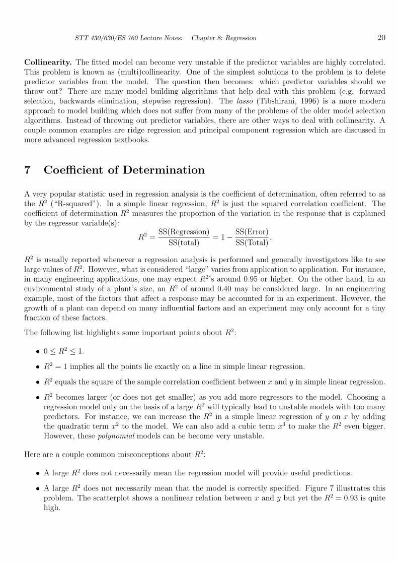
• A large R2 does not necessarily mean that the model is correctly specified. Figure 7 illustrates thisproblem. The scatterplot shows a nonlinear relation between x and y but yet the R2 = 0.93 is quitehigh.


0 2 4 6 8 10

02

46

810

x

y

R2 = 0.93

Figure 7: Scatterplot showing a nonlinear relationship between x and y but yet the R2 = 0.93. Thus, ahigh R2 does not necessarily mean the relation is linear.


8 Conclusion

This chapter presented a brief overview of regression analysis. As pointed out in the notes, there are severalmore advanced topics in regression analysis. Regression analysis can handle more complicated models thanthose presented here. For instance, nonlinear regression analysis can be used to model complicated (ornon-complicated) nonlinear relations. These nonlinear models typically require numerical algorithms tofind estimators. Often the relation between a response variable and a predictor is completely unknown. Abranch of regression analysis called nonparametric regression can be used to allow the data to determinethe shape of a regression curve. Multivariate regression is used to model several response variables as afunction of one or more predictor variables. Binary indicator variables can be added to regression modelsto allow the model to distinguish between different groups (e.g. male & female) in the population – thisleads to analysis of covariance. Functional data analysis is another branch of statistics where each datapoint is a curve. For instance, in a clinical study, subjects may be observed over time and a curve can beestimated for each individual subject to model the subject’s response to treatment over time.

9 Problems

1. It is well known that the height of a plant depends on the amount of fertilizer the plant receives.A study was done by varying the amount of fertilizer plants received and the heights of each ofthe plants were the measured. The correlation between the amount of fertilizer and the heights ofthe plants was found to not differ significantly from zero (this is equivalent to testing if the slopein a regression analysis differs significantly from zero). The experimenter was expecting to see asignificant positive correlation. Can you suggest two possible explanations why the correlation didnot differ significantly from zero?

2. The Federal Trade Commission rates different brands of domestic cigarettes. In their study, theymeasured the amount of carbon monoxide (co) in mg. and the amount of nicotine (mg.) producedby a burning cigarette of each brand. A simple linear regression model was run in SAS using co asthe dependent variable and nicotine as the independent (or predictor) variable. The output is shownbelow – use this output to answer the questions below.

Analysis of VarianceSum of Mean


Model 1 462.25591 462.25591 138.27 <.0001Error 23 76.89449 3.34324Corrected Total 24 539.15040

Root MSE 1.82845 R-Square 0.8574Dependent Mean 12.52800 Adj R-Sq 0.8512Coeff Var 14.59493

Parameter Estimates

Parameter Standard



Intercept 1 1.66467 0.99360 1.68 0.1074nicotine 1 12.39541 1.05415 11.76 <.0001

a) How many cigarette brands did the Federal Trade Commission evaluate?

b) What percentage of variation in carbon monoxide is explained by the amount of nicotine?

c) Write down the least-squares regression equation.

d) Does the amount of carbon monoxide produced by a burning cigarette depend on how muchnicotine is in the cigarette? Perform an appropriate hypothesis test to answer this question. Besure to define any parameters you use. Base you conclusion on the p-value of the test.

e) Give an estimate of how much carbon monoxide increases on average for each additional mil-ligram of nicotine in the cigarette.

f) What is the predicted amount of carbon monoxide produced by a cigarette containing 1.5 mgof nicotine?

3. A recent study investigated the concentration y of arsenic in the soil (measured in mg/kg) and thedistance x from a smelter plant (in meters). A simple linear regression model y = β0 + β1x + ε wasused to model the relationship between these two variables. The data from the study was used to testthe hypothesis of H0 : β1 = 0 versus H0 : β1 < 0 at a significance level α = 0.05. Do the followingparts:

a) In the context of this problem, what would be a type I error?

b) In the context of this problem, what is a type II error?

c) The least-squares regression line was found to be y = 60.2− 5.1x and the standard error of theestimated slope was found to be 1.32. What is the value of the t-test statistic for testing thehypothesis in this problem?

e) The null hypothesis was rejected in this test at α = 0.05. Write a sentence interpreting theestimated slope in the context of this problem.

4. The SAS program chlorophyll.sas in the Appendix has data on the concentration of chlorophyll-a in alake along with the concentration of phosphorus and nitrogen in the lake (Source: Smith and Shapiro1981). Chlorophyll-a is used as an indicator of water quality that measures the density algal cells.Phosphorus and nitrogen stimulate algal growth. The purpose of this homework is to use a simplelinear regression model to model the relationship between log(chlorophyll-a) and log(phosphorus) inthe lake. To obtain answers to the questions, run the SAS program.

a) Write down the equation for the estimated least-squares regression line relating logarithm ofchlorophyll-a to log(phosphorus).

b) Write a sentence that interprets the estimated slope in the context of this problem.

c) What is the estimated standard error of the estimated slope of the regression line?

d) SAS reports a t-statistic value of t = 10.81 associated with log(phosphorus). Write down theregression model and write out the null and alternative hypothesis that is being tested with thist-test statistic.

e) Write a sentence interpreting the p-value that is associated with the test statistic in part (e).


f) Compute a 95% confidence interval for the slope of the regression line and write a sentenceinterpreting this confidence interval.

5. Data on the velocity of water versus depth in a channel were acquired at a station below the GrandCoulee Dam at a distance of 13 feet from the edge of the river. Modeling water velocity in a channelis important when calculating river discharge. (Reference: Savini, J. and Bodhaine, G. L. (1971),Analysis of current meter data at Columbia River gaging stations, Washington and Oregon; USGSWater Supply Paper 1869-F.) Run the SAS program ColumbiaRiver.sas (which contains the data)in the Appendix to do the following parts:

a) Write down the equation for the estimated least-squares regression line relating water velocityto depth.

b) What is the estimated water velocity at the surface of the channel?

c) Find a 95% confidence interval for the slope of the regression line. Write a sentence thatinterprets this confidence interval in the context of this problem.

d) Generate a plot of the data along with the least-squares regression line and attach it to thisassignment. Does the relation between water depth and water velocity appear linear?

References.

Alaa r. Mostafa, Assem O. Barakat, Yaorong Qian, Terry L. Wade, Dongxing Yuan, (2004), “An Overviewof Metal Pollution in the Western Harbour of Alexandria, Egypt”, Soil & Sediment Contamination, 13,299311.

Tibshirani, R. (1996). Regression shrinkage and selection via the lasso. J. Royal. Statist. Soc B., Vol. 58,No. 1, pages 267-288)

10 Appendix

/*************************************************************

Chlorophyll-a in Lakes

Source: Smith and Shapiro (1981) in Environmental Science and

Technology, volume 15, pages 444-451.

Data:

Column 1: Chlorophyll-a

Column 2: Phosphorus

Column 3: Nitrogren

************************************************************/

data lake;

input chlor phos nitro;

logc=log(chlor);

logp=log(phos);

logn=log(nitro);

datalines;

95.0 329.0 8

39.0 211.0 6


27.0 108.0 11

12.9 20.7 16

34.8 60.2 9

14.9 26.3 17

157.0 596.0 4

5.1 39.0 13

10.6 42.0 11

96.0 99.0 16

7.2 13.1 25

130.0 267.0 17

4.7 14.9 18

138.0 217.0 11

24.8 49.3 12

50.0 138.0 10

12.7 21.1 22

7.4 25.0 16

8.6 42.0 10

94.0 207.0 11

3.9 10.5 25

5.0 25.0 22

129.0 373.0 8

86.0 220.0 12

64.0 67.0 19

;

proc print;

run;

proc reg;

model logc = logp;

output out=a p=p r=r;

run;

proc plot;

plot r*p/vref=0;

quit;

/****************************************************************

COLUMBIA RIVER VELOCITY-DEPTH

Data on the velocity (ft/sec) of water versus depth (feet)

in a channel were acquired at a station below

the Grand Coulee Dam at a distance of 13 feet from the edge of

the river. Modeling water velocity in a channel is important when

calculating river discharge. (Reference: Savini, J. and Bodhaine, G. L.

(1971), Analysis of

current meter data at Columbia River gaging stations, Washington and

Oregon; USGS Water Supply Paper 1869-F.)

***********************************************************************/


options ls=76;

data water;

input depth velocity;

datalines;

0.7 1.55

2.0 1.11

2.6 1.42

3.3 1.39

4.6 1.39

5.9 1.14

7.3 0.91

8.6 0.59

9.9 0.59

10.6 0.41

11.2 0.22

;

run;

proc reg;

model velocity = depth;

run;

quit;

Chapter 8: Regression - Wright State Universitythaddeus.tarpey/stt630chap8.pdf · In the simple...

Documents

Transcript of Chapter 8: Regression - Wright State Universitythaddeus.tarpey/stt630chap8.pdf · In the simple...