AP Statistics3.3 Least-Squares Regression

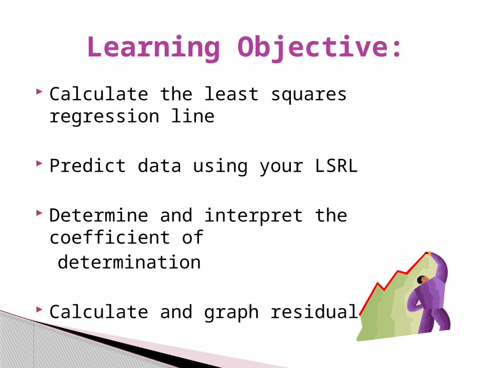
Calculate the least squares regression line

Predict data using your LSRL

Determine and interpret the coefficient of determination

Calculate and graph residual plots

Learning Objective:

If there is a linear relationship, we summarize this overall pattern by drawing a line through the scatterplot.

Least-squares regression is a method for finding a line that summarizes the relationship between two variables, but only in a linear setting.

Correlation measures the strength and direction of the linear relationship

between any two quantitative variables.

A regression line is a straight line that describes how a response variable y changes as an explanatory variable x changes. We often use a regression line to predict the value of y for a given value of x.

Regression, unlike correlation, requires that we have an explanatory variable and a response variable.

** We use this line to show a linear trend.

(Ex: We can find the correlation Between your GPA and # of siblings,but we don’t find a regression line to predict data. Do you really want your GPA predicted from the # of siblings you have!!!)

Error= Observed – Predicted

Example: We predict the height of a ladder to be 4.9ft, but it is actually 5.1 ft. Find the error.

Error= O- P= 5.1- 4.9 = 0.2 ft.A better term for your error is residual.

***A positive residual=prediction was to small***

When using LSRL, we need to find our error.

The Least-squares regression line of y on x is the line that makes the sum of the squares of the vertical distances of the data points from the line as small as possible.

(This is because we are comparing the observed y value to the predicted y value-not our x values)

y= observed response and

predicted response (“y hat”)

How to find the LSRL on your calculator.

Input: x into L1 y into L2

Stat-calc-8(linReg(ax+b))

*we use 8 not 4 like you did in AlgebraIn Algebra we used y=mx+b where b=y-int.In stat we use y=a+bx where b=slope.

How to find the LSRL on your calculator. # of

sneakers owned

Amount of exercise per week

1 2

3 5

7 16

13 30

TI-84: Stat-calc-8 (use 8 not 4)Xlist:L1Ylist:L2FreqList: (leave this blank)Store RegEQ: Y1 (vars-Yvars-1-1)Calculate

TI-83: Stat-calc-8 (use 8 not 4) then type in L1,L2, Y1, enter

-1.11+2.39x where x=#of sneakersy=amt. of exercise

# of sneakers owned

Amount of exercise per week

1 2

3 5

7 16

13 30

Use this data to predict the amount of exercise per week when you own 7 pairs of sneakers.

y(7)= -1.11+2.39(7)=15.64The easy way to do this on your calc since you

already told the calc to put the eq. into your y1: Go to a clear home screen.Vars-yvars-function-y1On your home screen you’ll have a y1. Type y1(7), hit enter

What is the residual? (Remember Residual=Obs. –Pred.)Residual= 16-15.64= 0.36

# of sneakers owned

Amount of exercise per week

1 2

3 5

7 16

13 30

Interpret the slope and y-intercept in context of the problem:

Slope: On average, for every change in x , y changes by b .

Y-intercept: When x=0, we predict y to be

a .*we need to put the words on average and we predict

because the line doesn’t touch every point, so the slope and y-int are not exactly what is happening, just estimates.

Slope and y-intercept

-1.11+2.39x Slope: On average, for every pair of sneakers you own , there is an

2.39 increase in the number of hours you exercise per week 

Y-intercept: When you don’t own any sneakers, we predict you to

exercise -1.11 hours

Does the y-int make sense in this problem?NO!! You can’t exercise negative hours

Use the data from the sneaker/exercise problem

We are given: r,

*** The point always falls directly on your line of best fit****

The least-squares regression line is the line:

With slope

And intercept

 

Equation of the Least-squares Regression Line (if we don’t have all

the data points to plot)

Suppose we have an explanatory (standing reach)and response variable (jumping reach) and we know:

Even though we don’t know the actual data, we can still construct the equation for the least-squares line and use it to make predictions.

Example:

b= 0.9952(.9/.6) = 1.4928

a= 7.3-(1.4928)(5.1)= -.3133

therefore -.3133 + 1.4928x

(Hint: Don’t forget to define your variables!)x= standing reachy= jumping reach 

 Slope:

On average, for every increase of your standing reach, there is an 1.49 increase in your jumping reach

 

Y-intercept:

When your standing reach is 0, we predict your jumping reach to be -0.333.

Interpret

  The coefficient of determination, , is the fraction of the variation in the values of y that is explained by least-squares regression of y on x.

In other words:

% of the change in y can be explained by the change in x .

What does in regression do?

# of hours studied

Test grade

1 72

2 80

3 87

4 94

5 90

Find the coefficient of determination

# of hours practiced

# of wins

0 4

1 3

2 1

4 8

6 9

Find the coefficient of determination

Fact 1: we find slope and intercept by using means, standard deviations, an correlation.

Fact2: we use the regression line to predict y for any given x

  Fact 3:recognize outliers and potentially

influential points   Fact 4:we use the regression line to

calculate residuals. (we look for patterns)

Facts about least-squares regression

Predict data outside our realm of data given.

Example: Predict gas prices for 2012

Extrapolation

year Ave. gas price

2001 $1.09

2004 $2.89

2007 $3.15

2011 $3.70

- the difference between an observed value of the response variable and the value predicted by the regression line. That is:

Residual= observed y – predicted y =

Residuals

The sum of the residuals is always 0!!

What do we know about the residuals from the least-squares regression line?

Step 1: Input Data into L₁ and L₂Step 2: STAT/CALC/8/ENTERStep 3: LinReg(a+bx) L₁,L₂, Y₁Then go back into your lists and input L3L3= Obs-Pred=L2-y1(L1)

Plot: L₁, L₃ Don’t forget to label your x axis with your x and your

y-axis is your residuals.

How to construct a residual plot using your calculator?

L₁ L₂ L₃X Y L₂- Y₁(L₁)

Follow each step exactly!!

Create a residual plot

# of hours practiced

# of wins

0 4

1 3

2 1

4 8

6 9

1- A curved pattern

2- Increasing or Decreasing pattern

3- Outliers or influential points

Any pattern in a residual plot tells us it’s NOT a good linear fit

Here’s what to look for when you examine residuals, using either a

scatterplot of the data or a residual plot.

Outlier- Influential-

Outliers and influential observations in regression