CHAPTER 8: Nonparametric Methods Alpaydin transparencies significantly modified, extended and...

CHAPTER 8:

Nonparametric Methods

Alpaydin transparencies significantly modified, extended and changed by Ch. Eick

Last updated: March 4, 2011

Eick/Alpaydin: Non-Parametric Density Estimation 2

Non-Parametric Density Estimation Goal is to obtain a density function:

http://en.wikipedia.org/wiki/Probability_density_function

Parametric (single global model), semiparametric (small number of local models)

Nonparametric: Similar inputs have similar outputs Keep the training data;“let the data speak for itself” Given x, find a small number of closest training

instances and interpolate from these Aka lazy/memory-based/case-based/instance-based

learning



Histograms Histogram

Usually shows the distribution of values of a single variable Divide the values into bins and show a bar plot of the

number of objects in each bin. The height of each bar indicates the number of objects Shape of histogram depends on the number of bins

Example: Petal Width (10 and 20 bins, respectively)

Lecture Notes for E Alpaydın 2004 Introduction to Machine Learning © The MIT Press (V1.1)4

Density Estimation

Given the training set X={xt}t drawn iid from p(x) Divide data into bins of size h, stating from origin xo

Histogram:

Naive estimator:

or

Nh

xxxpt asbin same in the #ˆ

Nh

hxxhxxpt 2/2/#ˆ

otherwise01if 21 1

1

u/uwh

xxwNh

xpN

t

t

Typo corrected on March 5 2011


Origin 0; h(1)=4/16

h(1.25)=1/8


h(2)=2/2*8=0.125

7

Gaussian Kernel Estimator Kernel function, e.g., Gaussian kernel:

Kernel estimator (Parzen windows):

Gaussian Influence Functions in general:

N

t

t

hxxdK

Nhxp

1

),(1ˆ

2exp

21 2uuK

Influence of xt on x; h determines how quickly influence decreases as distance between xt and x increases; h is called “width” of kernel.

Eick/Alpaydin: Non-Parametric Density Estimation

Query point

hbadbaluence

2),(exp

21),(inf

2

8

Example: Kernel Density Estimation

D={x1,x2,x3,x4}fD

Gaussian(x)= influence(x1,x) + influence(x2,x) + influence(x3,x) + influence(x4,x)= 0.04+0.06+0.08+0.6=0.78x1

x2

x3

x4x 0.6

0.08

0.06

0.04

y

Remark: the density value of y would be larger than the one for xEick/Alpaydin: Non-Parametric Density Estimation

2)/)((exp

21,

2

infhbabaluence

10

Density Functions for different values of h/

Remark:

Eick/Alpaydin: Non-Parametric Density Estimation


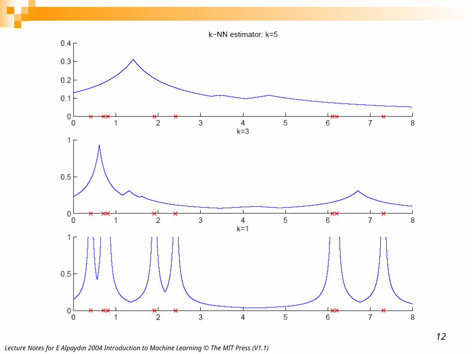
k-Nearest Neighbor Estimator

Instead of fixing bin width h and counting the number of instances, fix the instances (neighbors) k and check bin width

dk(x), distance to kth closest instance to x

xNdkxpk2

ˆ


Multivariate Data Kernel density estimator

Multivariate Gaussian kernel

spheric

ellipsoid

N

t

t

d hK

Nhp

1

1 xxx

uuu

uu

1212

2

21exp

21

2exp21

SS

T//d

d

K

K


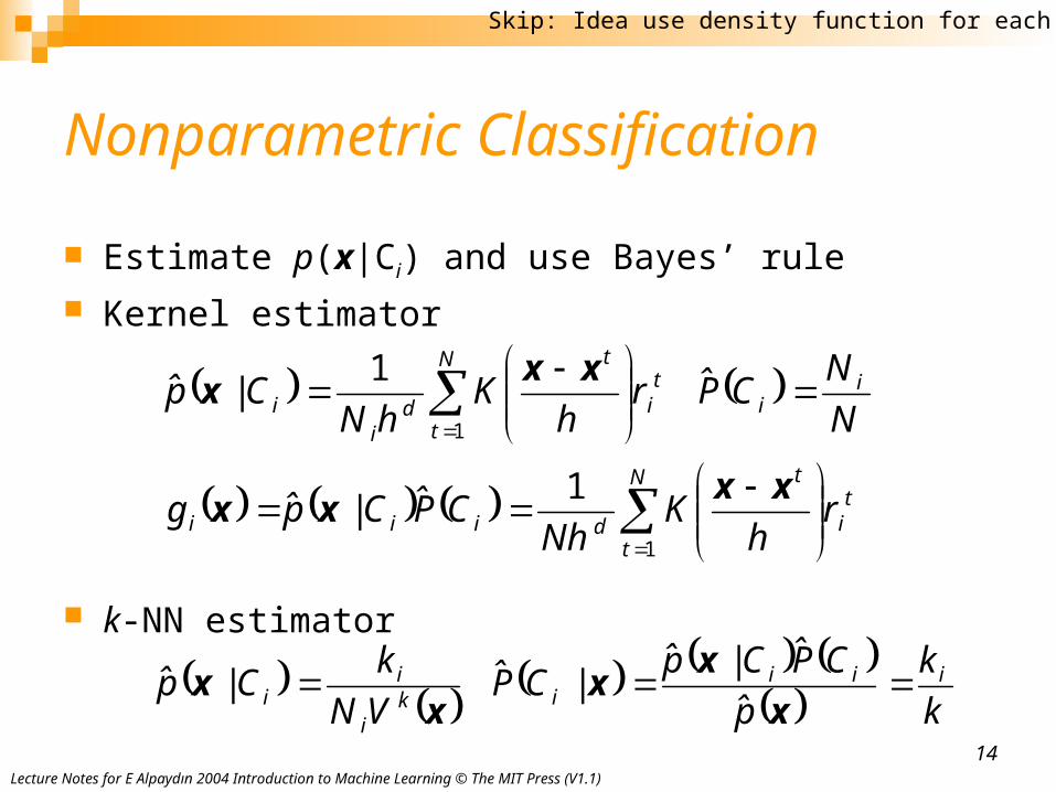
Nonparametric Classification

Estimate p(x|Ci) and use Bayes’ rule Kernel estimator

k-NN estimator

ti

N

t

t

diii

ii

ti

N

t

t

di

i

rh

KNh

CPCpg

NNCPr

hK

hNCp

1

1

1|

1|

xxxx

xxx

k

kp

CPCpCPVNkCp iii

iki

ii

xxx

xx || |

Skip: Idea use density function for each class


Condensed Nearest Neighbor

Time/space complexity of k-NN is O (N) Find a subset Z of X that is small and is accurate

in classifying X (Hart, 1968)

ZZXXZ || E'E

skip


Condensed Nearest Neighbor

Incremental algorithm: Add instance if needed

skip


Nonparametric Regression Aka smoothing models Regressogram

otherwise0|-x| if1

,

otherwise0bin with same in the is if1

,

where,

,ˆ1

1

hxxxb

xxxxb

xxbrxxbxg

t

t

t

t

Nt

t

tNt

t

Idea: use averageof the output variable in a neighborhood of x


uses bins to define neighborhoods

19

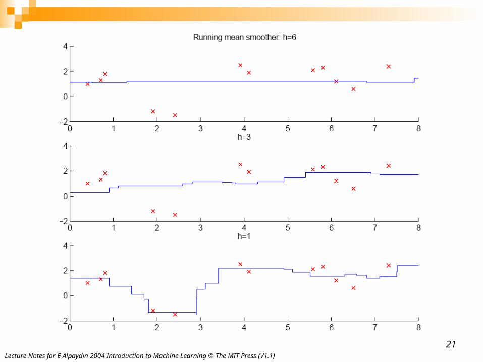
Running mean smoother

Running line smoother

Running Mean/Kernel Smoother

Kernel smoother

where K( ) is Gaussian

Additive models (Hastie and Tibshirani, 1990)

otherwise0 1if 1

where

1

1

uuw

hxxw

rh

xxwxg

N

t

t

tN

t

t

N

t

t

tN

t

t

hxxK

rhxxK

xg

1

1

ˆ

Idea: weights example inversely by their distance to x.


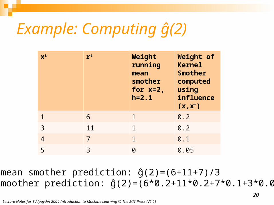
Example: Computing ĝ(2)xt rt Weight

running mean smother for x=2, h=2.1

Weight of Kernel Smother computed using influence(x,xt)

1 6 1 0.23 11 1 0.24 7 1 0.15 3 0 0.05

Running mean smother prediction: ĝ(2)=(6+11+7)/3Kernel smoother prediction: ĝ(2)=(6*0.2+11*0.2+7*0.1+3*0.05)/0.55


Idea: Uses influence function to determine weight

23

Smoothness/Smooth Functions depends on a function’s discontinuities and on how

quickly its first/second/third/… derivative changes A smooth function is a continuous function whose

derivatives change quite slowly Smooth function are frequently preferred as

models of systems and decision making small changes in input result in small changes in output

Design: Smooth surfaces are more appealing; e.g. car or sofa design

24

Choosing h/k When k or h is small, single instances matter; bias is

small, variance is large (undersmoothing): High complexity

As k or h increases, we average over more instances and variance decreases but bias increases (oversmoothing): Low complexity

h/k large: very few hills/smooth h/k small: a lot of hills; a lot of changes/discontinuities

in the first/second/third/… derivative Cross-validation is used to finetune k or h.

CHAPTER 8: Nonparametric Methods Alpaydin transparencies significantly modified, extended and...

Documents

Transcript of CHAPTER 8: Nonparametric Methods Alpaydin transparencies significantly modified, extended and...