Chapter 8: Confidence Intervals

Introduction

Suppose you are trying to determine the mean rent of a two-bedroom apartment in your town. You might look in the

classified section of the newspaper, write down several rents listed, and average them together. You would have

obtained a point estimate of the true mean.

If you are trying to determine the percent of times you make a basket when shooting a basketball, you might count the

number of shots you make and divide that by the number of shots you attempted. In this case, you would have obtained

a point estimate for the true proportion.

We use sample data to make generalizations about an unknown population. This part of statistics is called inferential

statistics.

The sample data help us to make an estimate of a population parameter.

The point estimate is most likely not the exact value of the population parameter, but close to it. After calculating point

estimates, we construct confidence intervals in which we believe the parameter lies.

In this chapter, you will learn to construct and interpret confidence intervals. You will also learn a new distribution, the

Student's-t, and how it is used with these intervals. Throughout the chapter, it is important to keep in mind that the

confidence interval is a random variable. It is the parameter that is fixed.

If you worked in the marketing department of an entertainment company, you might be interested in the mean number

of compact discs (CD's) a consumer buys per month.

If so, you could conduct a survey and calculate the sample mean, , and the sample standard deviation, s. You would

use to estimate the population mean and s to estimate the population standard deviation.

The sample mean, , is the point estimate for the population mean, μ.

The sample standard deviation, s, is the point estimate for the population standard deviation, σ.

Each of and s is also called a statistic.

A confidence interval is another type of estimate but, instead of being just one number, it is an interval of numbers. The

interval of numbers is a range of values calculated from a given set of sample data. The confidence interval is likely to

include an unknown population parameter.

Suppose for the CD example we do not know the population mean μ but we do know that the population standard

deviation is σ = 1 and our sample size is 100. Then by the Central Limit Theorem, the standard deviation for the sample

mean is

√

√

The Empirical Rule, which applies to bell-shaped distributions, says that in approximately 95% of the samples, the

sample mean, , will be within two standard deviations of the population mean μ.

For our CD example, two standard deviations is (2)(0.1) = 0.2. The sample mean is likely to be within 0.2 units of μ.

Because is within 0.2 units of μ, which is unknown, then μ is likely to be within 0.2 units of in 95% of the samples.

The population mean μ is contained in an interval between:

- 0.2 and + 0.2 in 95% of all the samples.

For the CD example, suppose that a sample produced a sample mean = 2. Then the unknown population mean μ is

between

− 0.2 = 2 − 0.2 = 1.8

and + 0.2 = 2 + 0.2 = 2.2

We say that we are 95% confident that the unknown population mean number of CDs is between 1.8 and 2.2.

The 95% confidence interval is (1.8, 2.2).

The 95% confidence interval implies two possibilities. Either the interval (1.8, 2.2) contains the true mean μ or our

sample produced an that is not within 0.2 units of the true mean μ. The second possibility happens for only 5% of all

the samples (100% - 95%).

Remember that a confidence interval is created for an unknown population parameter like the population mean, μ.

Confidence intervals for some parameters have the form

(point estimate - margin of error, point estimate + margin of error)

The margin of error depends on the confidence level or percentage of confidence.

When you read newspapers and journals, some reports will use the phrase "margin of error." Other reports will not use

that phrase, but include a confidence interval as the point estimate + or - the margin of error. These are two ways of

expressing the same concept.

Confidence Interval, Single Population Mean,

Population Standard Deviation Known, Normal

Calculating the Confidence Interval

To construct a confidence interval for a single unknown population mean μ, where the population standard deviation is

known, we need as an estimate for μ and we need the margin of error.

Here, the margin of error is called the error bound for a population mean (abbreviated EBM). The sample mean is

the point estimate of the unknown population mean μ

The confidence interval estimate will have the form:

(point estimate - error bound, point estimate + error bound) or,

in symbols,( − EBM, + EBM)

The margin of error depends on the confidence level (CL)

The confidence level is often considered the probability that the calculated confidence interval estimate will contain the

true population parameter.

It is more accurate to state that the confidence level is the percent of confidence intervals that contain the true

population parameter when repeated samples are taken. Most often, it is the choice of the person constructing the

confidence interval to choose a confidence level of 90% or higher because that person wants to be reasonably certain of

his or her conclusions.

There is another probability called alpha (α). α is related to the confidence level CL. α is the probability that the interval

does not contain the unknown population parameter.

Mathematically, α + CL = 1.

EXAMPLE 1

Suppose we have collected data from a sample. We know the sample mean but we do not know the mean for

the entire population.

The sample mean is 7 and the error bound for the mean is 2.5.

= 7 and EBM= 2.5.

The confidence interval is (7 − 2.5,7 + 2.5); calculating the values gives (4.5,9.5).

If the confidence level (CL) is 95%, then we say that "We estimate with 95% confidence that the true value of the

population mean is between 4.5 and 9.5."

A confidence interval for a population mean with a known standard deviation is based on the fact that the sample

means follow an approximately normal distribution. Suppose that our sample has a mean of = 10 and we have

constructed the 90% confidence interval (5, 15) where EBM=5.

To get a 90% confidence interval, we must include the central 90% of the probability of the normal distribution. If we

include the central 90%, we leave out a total of α = 10% in both tails, or 5% in each tail, of the normal distribution.

To capture the central 90%, we must go out 1.645 "standard deviations" on either side of the calculated sample mean.

1.645 is the z-score from a Standard Normal probability distribution that puts an area of 0.90 in the center, an area of

0.05 in the far left tail, and an area of 0.05 in the far right tail.

In this section, we need to use the standard deviation that applies to sample means, which is

√ . This is commonly

called the "standard error of the mean" in order to clearly distinguish the standard deviation for a mean from the

population standard deviation σ.

As a result of the Central Limit Theorem:

is normally distributed, ~ N(μX,

√ ).

When the population standard deviation σ is known, we use a Normal distribution to calculate the error bound.

Calculating the Confidence Interval:

To construct a confidence interval estimate for an unknown population mean, we need data from a random sample. The

steps to construct and interpret the confidence interval are:

Calculate the sample mean from the sample data. Remember, in this section, we already know the

population standard deviation σ.

Find the Z-score that corresponds to the confidence level.

Calculate the error bound EBM

Construct the confidence interval

Write a sentence that interprets the estimate in the context of the situation in the problem. (Explain what the

confidence interval means, in the words of the problem.)

We will first examine each step in more detail, and then illustrate the process with some examples.

Finding z for the stated Confidence Level

When we know the population standard deviation σ, we use a standard normal distribution to calculate the error

bound EBM and construct the confidence interval. We need to find the value of z that puts an area equal to the

confidence level (in decimal form) in the middle of the standard normal distribution Z~N(0,1).

The confidence level, CL, is the area in the middle of the standard normal distribution. CL = 1− α. So α is the area that is

split equally between the two tails. Each of the tails contains an area equal to α/2 .

The z-score that has an area to the right of α/2 is denoted by zα/2

For example, when CL = 0.95 then α = 0.05 and α/2 = 0.025; we write zα/2 = z.025

The area to the right of z.025 is 0.025 and the area to the left of z.025 is 1 - 0.025 = 0.975

zα/2 = z0.025 = 1.96 , using a calculator, computer or a Standard Normal probability table.

Using the TI83, TI83+ or TI84+ calculator:

invNorm(0.975,0,1) = 1.96

EBM: Error Bound

The error bound formula for an unknown population mean μ when the population standard deviation σ is known is

EBM= zα/2 ⋅

√

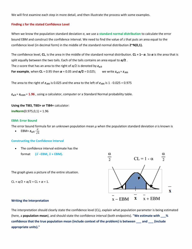
Constructing the Confidence Interval

The confidence interval estimate has the

format ( −EBM, + EBM).

The graph gives a picture of the entire situation.

CL + α/2 + α/2 = CL + α = 1.

Writing the Interpretation

The interpretation should clearly state the confidence level (CL), explain what population parameter is being estimated

(here, a population mean), and should state the confidence interval (both endpoints). "We estimate with ___%

confidence that the true population mean (include context of the problem) is between ___ and ___ (include

appropriate units)."

EXAMPLE 2

Suppose scores on exams in statistics are normally distributed with an unknown population mean and a population

standard deviation of 3 points. A random sample of 36 scores is taken and gives a sample mean (sample mean score) of

68. Find a confidence interval estimate for the population mean exam score (the mean score on all exams).

A: Find a 90% confidence interval for the true (population) mean of statistics exam scores.

You can use technology to directly calculate the confidence interval

The first solution is shown step-by-step (Solution A).

The second solution uses the TI-83, 83+ and 84+ calculators (Solution B).

a. Find the EBM (error bound for the mean)

b. Write the 90% confidence interval

c. Interpret your result

Changing the Confidence Level or Sample Size

EXAMPLE 3: Changing the Confidence Level

Suppose we change the original problem by using a 95% confidence level. Find a 95% confidence interval for the true

(population) mean statistics exam score.

a. Find the EBM

b. Write the 95% confidence interval

c. Interpret your result

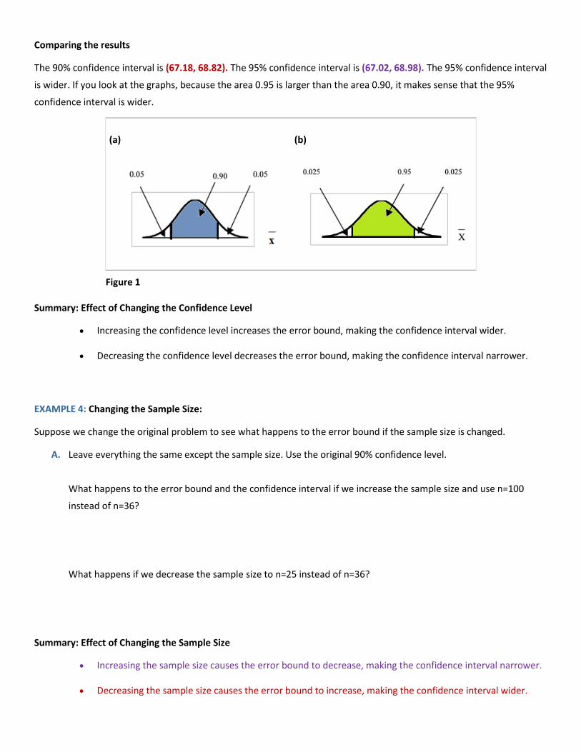
Comparing the results

The 90% confidence interval is (67.18, 68.82). The 95% confidence interval is (67.02, 68.98). The 95% confidence interval

is wider. If you look at the graphs, because the area 0.95 is larger than the area 0.90, it makes sense that the 95%

confidence interval is wider.

(a) (b)

Figure 1

Summary: Effect of Changing the Confidence Level

Increasing the confidence level increases the error bound, making the confidence interval wider.

Decreasing the confidence level decreases the error bound, making the confidence interval narrower.

EXAMPLE 4: Changing the Sample Size:

Suppose we change the original problem to see what happens to the error bound if the sample size is changed.

A. Leave everything the same except the sample size. Use the original 90% confidence level.

What happens to the error bound and the confidence interval if we increase the sample size and use n=100

instead of n=36?

What happens if we decrease the sample size to n=25 instead of n=36?

Summary: Effect of Changing the Sample Size

Increasing the sample size causes the error bound to decrease, making the confidence interval narrower.

Decreasing the sample size causes the error bound to increase, making the confidence interval wider.

Working Backwards to Find the Error Bound or Sample Mean

Working Backwards to find the Error Bound or the Sample Mean

When we calculate a confidence interval, we find the sample mean and calculate the error bound and use them to

calculate the confidence interval. But sometimes when we read statistical studies, the study may state the confidence

interval only. If we know the confidence interval, we can work backwards to find both the error bound and the sample

mean.

Finding the Error Bound

From the upper value for the interval, subtract the sample mean

OR, from the upper value for the interval, subtract the lower value. Then divide the difference by 2.

Finding the Sample Mean

Subtract the error bound from the upper value of the confidence interval

OR, Average the upper and lower endpoints of the confidence interval

Notice that there are two methods to perform each calculation. You can choose the method that is easier to use with

the information you know.

EXAMPLE 5

Suppose we know that a confidence interval is (67.18, 68.82) and we want to find the error bound. We may know that

the sample mean is 68. Or perhaps our source only gave the confidence interval and did not tell us the value of the

sample mean.

a. Calculate the Error Bound:

b. Calculate the Sample Mean:

Calculating the Sample Size n

If researchers desire a specific margin of error, then they can use the error bound formula to calculate the required

sample size.

The error bound formula for a population mean when the population standard deviation is known is EBM = zα/2 ⋅

√

The formula for sample size is n = z2σ2/EBM2, found by solving the error bound formula for n.

In this formula, z is zα/2, corresponding to the desired confidence level. A researcher planning a study who wants a

specified confidence level and error bound can use this formula to calculate the size of the sample needed for the study.

EXAMPLE 6

The population standard deviation for the age of Foothill College students is 15 years. If we want to be 95% confident

that the sample mean age is within 2 years of the true population mean age of Foothill College students , how many

randomly selected Foothill College students must be surveyed?

Confidence Interval, Single Population Mean, Standard Deviation Unknown, Student's-t

In practice, we rarely know the population standard deviation. In the past, when the sample size was large, this did not

present a problem to statisticians. They used the sample standard deviation s as an estimate for σ and proceeded as

before to calculate a confidence interval with close enough results.

However, statisticians ran into problems when the sample size was small. A small sample size caused inaccuracies in the

confidence interval.

William S. Gossett (1876-1937) of the Guinness brewery in Dublin, Ireland ran into this problem.

His experiments with hops and barley produced very few samples. Just replacing σ with s did not produce accurate

results when he tried to calculate a confidence interval. He realized that he could not use a normal distribution for the

calculation; he found that the actual distribution depends on the sample size.

This problem led him to "discover" what is called the Student's-t distribution. The name comes from the fact that

Gosset wrote under the pen name "Student."

Up until the mid 1970s, some statisticians used the normal distribution approximation for large sample sizes and only

used the Student's-t distribution for sample sizes of at most 30. With the common use of graphing calculators and

computers, the practice is to use the Student's-t distribution whenever s is used as an estimate for σ.

If you draw a simple random sample of size n from a population that has approximately a normal distribution with

mean μ and unknown population standard deviation σ and calculate the t-score:

√ ,

Then the t-scores follow a Student's-t distribution with n – 1 degrees of freedom. The t-score has the same

interpretation as the z-score. It measures how far is from its mean μ. For each sample size n there is a different

Student's-t distribution.

The degrees of freedom, n – 1, come from the calculation of the sample standard deviation s.

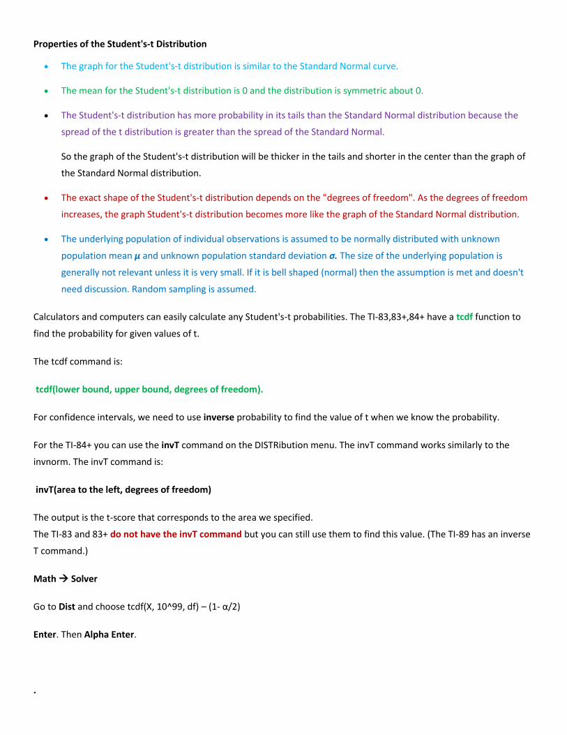
Properties of the Student's-t Distribution

The graph for the Student's-t distribution is similar to the Standard Normal curve.

The mean for the Student's-t distribution is 0 and the distribution is symmetric about 0.

The Student's-t distribution has more probability in its tails than the Standard Normal distribution because the

spread of the t distribution is greater than the spread of the Standard Normal.

So the graph of the Student's-t distribution will be thicker in the tails and shorter in the center than the graph of

the Standard Normal distribution.

The exact shape of the Student's-t distribution depends on the "degrees of freedom". As the degrees of freedom

increases, the graph Student's-t distribution becomes more like the graph of the Standard Normal distribution.

The underlying population of individual observations is assumed to be normally distributed with unknown

population mean μ and unknown population standard deviation σ. The size of the underlying population is

generally not relevant unless it is very small. If it is bell shaped (normal) then the assumption is met and doesn't

need discussion. Random sampling is assumed.

Calculators and computers can easily calculate any Student's-t probabilities. The TI-83,83+,84+ have a tcdf function to

find the probability for given values of t.

The tcdf command is:

tcdf(lower bound, upper bound, degrees of freedom).

For confidence intervals, we need to use inverse probability to find the value of t when we know the probability.

For the TI-84+ you can use the invT command on the DISTRibution menu. The invT command works similarly to the

invnorm. The invT command is:

invT(area to the left, degrees of freedom)

The output is the t-score that corresponds to the area we specified.

The TI-83 and 83+ do not have the invT command but you can still use them to find this value. (The TI-89 has an inverse

T command.)

Math Solver

Go to Dist and choose tcdf(X, 10^99, df) – (1- α/2)

Enter. Then Alpha Enter.

.

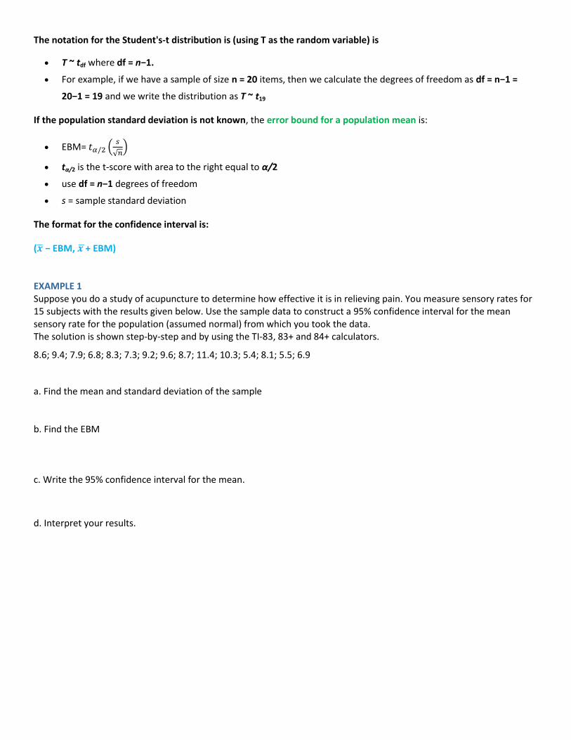
The notation for the Student's-t distribution is (using T as the random variable) is

T ~ tdf where df = n−1.

For example, if we have a sample of size n = 20 items, then we calculate the degrees of freedom as df = n−1 =

20−1 = 19 and we write the distribution as T ~ t19

If the population standard deviation is not known, the error bound for a population mean is:

EBM= (

√ )

tα/2 is the t-score with area to the right equal to α/2

use df = n−1 degrees of freedom

s = sample standard deviation

The format for the confidence interval is:

( − EBM, + EBM) EXAMPLE 1 Suppose you do a study of acupuncture to determine how effective it is in relieving pain. You measure sensory rates for 15 subjects with the results given below. Use the sample data to construct a 95% confidence interval for the mean sensory rate for the population (assumed normal) from which you took the data. The solution is shown step-by-step and by using the TI-83, 83+ and 84+ calculators.

8.6; 9.4; 7.9; 6.8; 8.3; 7.3; 9.2; 9.6; 8.7; 11.4; 10.3; 5.4; 8.1; 5.5; 6.9

a. Find the mean and standard deviation of the sample b. Find the EBM c. Write the 95% confidence interval for the mean.

d. Interpret your results.

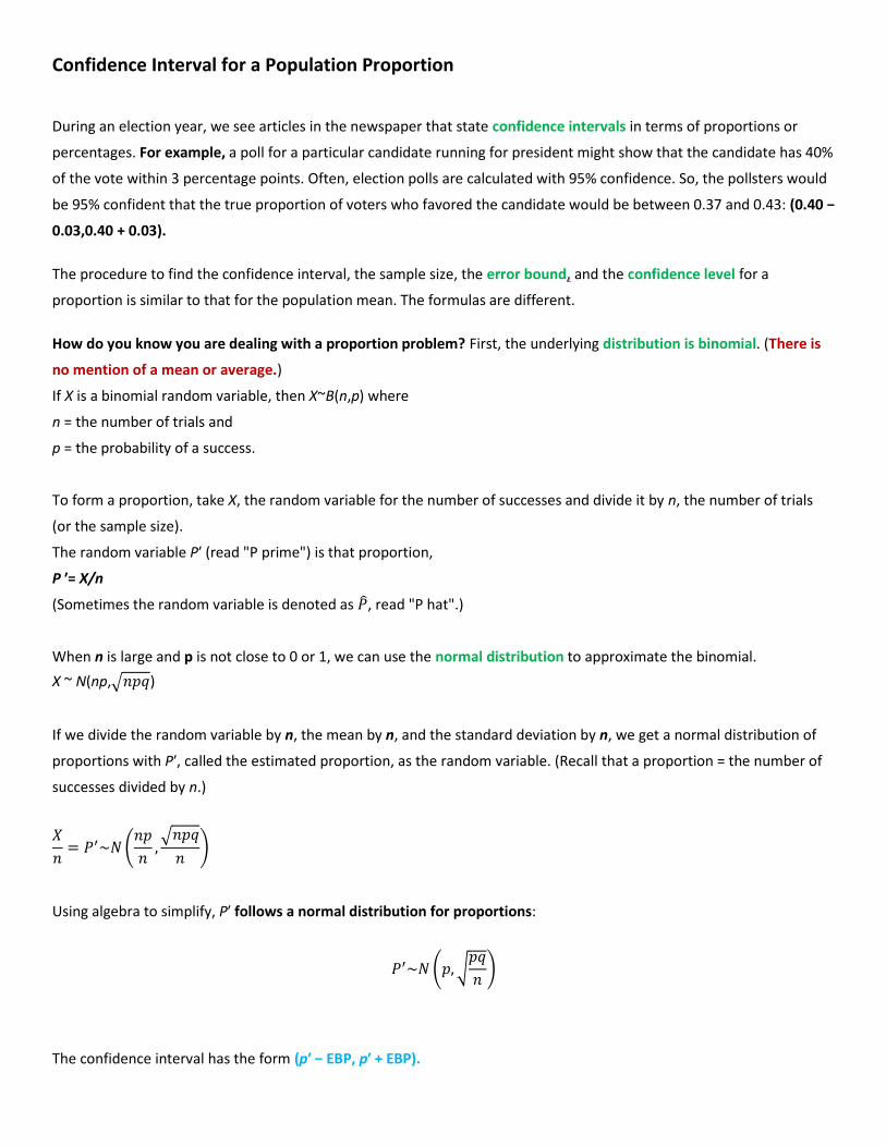
Confidence Interval for a Population Proportion

During an election year, we see articles in the newspaper that state confidence intervals in terms of proportions or

percentages. For example, a poll for a particular candidate running for president might show that the candidate has 40%

of the vote within 3 percentage points. Often, election polls are calculated with 95% confidence. So, the pollsters would

be 95% confident that the true proportion of voters who favored the candidate would be between 0.37 and 0.43: (0.40 −

0.03,0.40 + 0.03).

The procedure to find the confidence interval, the sample size, the error bound, and the confidence level for a

proportion is similar to that for the population mean. The formulas are different.

How do you know you are dealing with a proportion problem? First, the underlying distribution is binomial. (There is

no mention of a mean or average.)

If X is a binomial random variable, then X~B(n,p) where

n = the number of trials and

p = the probability of a success.

To form a proportion, take X, the random variable for the number of successes and divide it by n, the number of trials

(or the sample size).

The random variable P′ (read "P prime") is that proportion,

P ′= X/n

(Sometimes the random variable is denoted as , read "P hat".)

When n is large and p is not close to 0 or 1, we can use the normal distribution to approximate the binomial.

X ~ N(np,√ )

If we divide the random variable by n, the mean by n, and the standard deviation by n, we get a normal distribution of

proportions with P′, called the estimated proportion, as the random variable. (Recall that a proportion = the number of

successes divided by n.)

(

√

)

Using algebra to simplify, P′ follows a normal distribution for proportions:

( √

)

The confidence interval has the form (p′ − EBP, p′ + EBP).

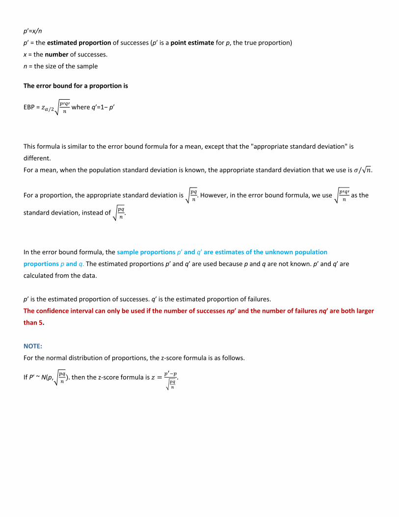
p′=x/n

p′ = the estimated proportion of successes (p′ is a point estimate for p, the true proportion)

x = the number of successes.

n = the size of the sample

The error bound for a proportion is

EBP = √

where q′=1− p′

This formula is similar to the error bound formula for a mean, except that the "appropriate standard deviation" is

different.

For a mean, when the population standard deviation is known, the appropriate standard deviation that we use is √ .

For a proportion, the appropriate standard deviation is √

However, in the error bound formula, we use √

as the

standard deviation, instead of √

In the error bound formula, the sample proportions p′ and q′ are estimates of the unknown population

proportions p and q. The estimated proportions p′ and q′ are used because p and q are not known. p′ and q′ are

calculated from the data.

p′ is the estimated proportion of successes. q′ is the estimated proportion of failures.

The confidence interval can only be used if the number of successes np′ and the number of failures nq′ are both larger

than 5.

NOTE:

For the normal distribution of proportions, the z-score formula is as follows.

If P′ ~ N(p,√

then the z-score formula is

√

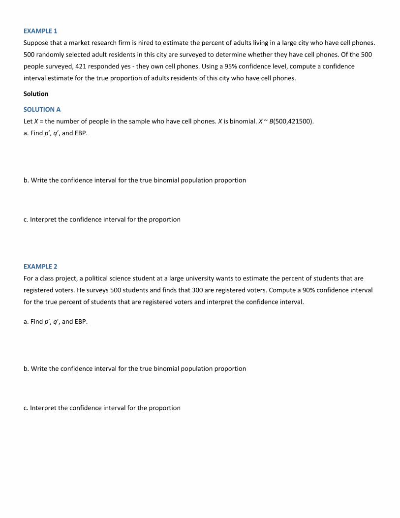
EXAMPLE 1

Suppose that a market research firm is hired to estimate the percent of adults living in a large city who have cell phones.

500 randomly selected adult residents in this city are surveyed to determine whether they have cell phones. Of the 500

people surveyed, 421 responded yes - they own cell phones. Using a 95% confidence level, compute a confidence

interval estimate for the true proportion of adults residents of this city who have cell phones.

Solution

SOLUTION A

Let X = the number of people in the sample who have cell phones. X is binomial. X ~ B(500,421500).

a. Find p′, q′, and EBP.

b. Write the confidence interval for the true binomial population proportion

c. Interpret the confidence interval for the proportion

EXAMPLE 2

For a class project, a political science student at a large university wants to estimate the percent of students that are

registered voters. He surveys 500 students and finds that 300 are registered voters. Compute a 90% confidence interval

for the true percent of students that are registered voters and interpret the confidence interval.

a. Find p′, q′, and EBP.

b. Write the confidence interval for the true binomial population proportion

c. Interpret the confidence interval for the proportion

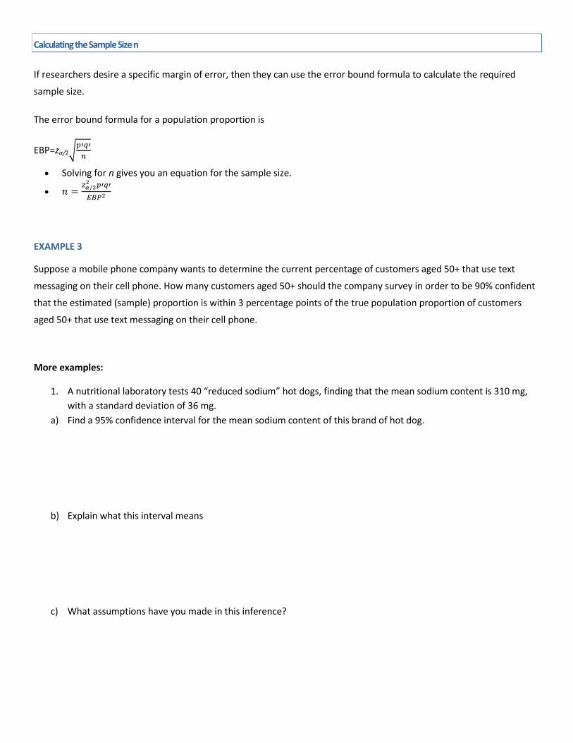
Calculating the Sample Size n

If researchers desire a specific margin of error, then they can use the error bound formula to calculate the required

sample size.

The error bound formula for a population proportion is

EBP=zα/2√

Solving for n gives you an equation for the sample size.

EXAMPLE 3

Suppose a mobile phone company wants to determine the current percentage of customers aged 50+ that use text

messaging on their cell phone. How many customers aged 50+ should the company survey in order to be 90% confident

that the estimated (sample) proportion is within 3 percentage points of the true population proportion of customers

aged 50+ that use text messaging on their cell phone.

More examples:

1. A nutritional laboratory tests 40 “reduced sodium” hot dogs, finding that the mean sodium content is 310 mg,

with a standard deviation of 36 mg.

a) Find a 95% confidence interval for the mean sodium content of this brand of hot dog.

b) Explain what this interval means

c) What assumptions have you made in this inference?

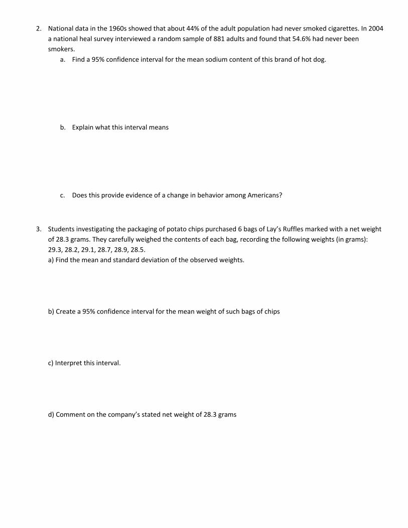
2. National data in the 1960s showed that about 44% of the adult population had never smoked cigarettes. In 2004

a national heal survey interviewed a random sample of 881 adults and found that 54.6% had never been

smokers.

a. Find a 95% confidence interval for the mean sodium content of this brand of hot dog.

b. Explain what this interval means

c. Does this provide evidence of a change in behavior among Americans?

3. Students investigating the packaging of potato chips purchased 6 bags of Lay’s Ruffles marked with a net weight

of 28.3 grams. They carefully weighed the contents of each bag, recording the following weights (in grams):

29.3, 28.2, 29.1, 28.7, 28.9, 28.5.

a) Find the mean and standard deviation of the observed weights.

b) Create a 95% confidence interval for the mean weight of such bags of chips

c) Interpret this interval.

d) Comment on the company’s stated net weight of 28.3 grams