6.1 Confidence Intervals for the Mean (Large Samples) Statistics Spring Semester Mrs. Spitz.
Upload
santiago-blacklidgeCategory
view
245download
4
Confidence Intervals
Chapter 6
§ 6.1
Confidence Intervals for the Mean (Large
Samples)
3
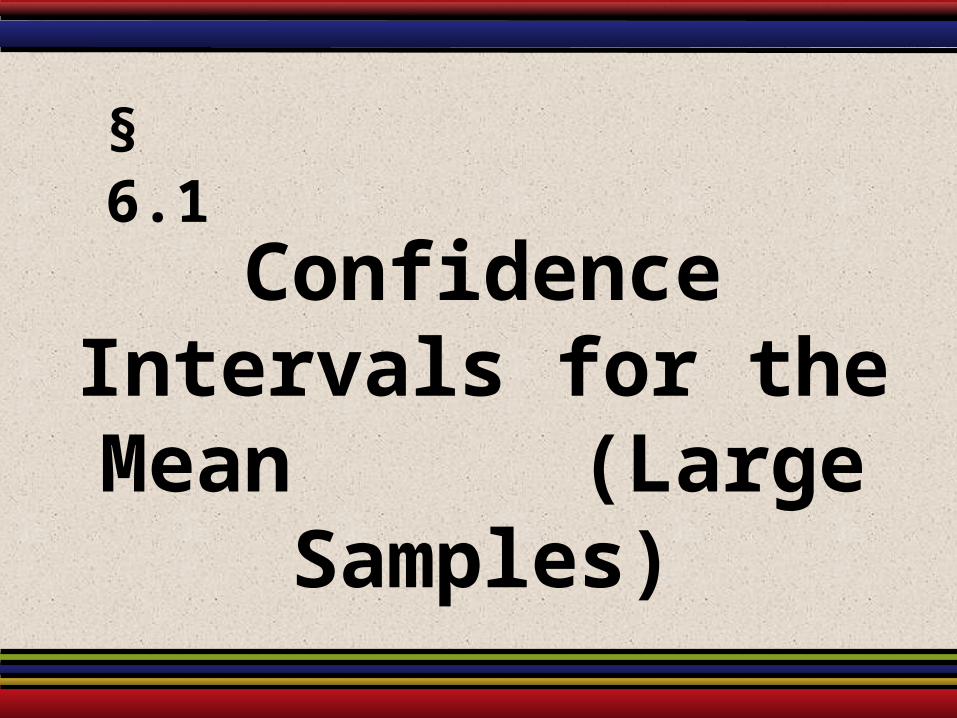
Point Estimate for Population μ
A point estimate is a single value estimate for a population parameter. The most unbiased point estimate of the population mean, , is the sample mean, .Example:A random sample of 32 textbook prices (rounded to the nearest dollar) is taken from a local college bookstore. Find a point estimate for the population mean, .
34 34 38 45 45 45 45 5456 65 65 66 67 67 68 7479 86 87 87 87 88 90 9094 95 96 98 98 101 110 121
The point estimate for the population mean of textbooks in the bookstore is $74.22.
74.22
4
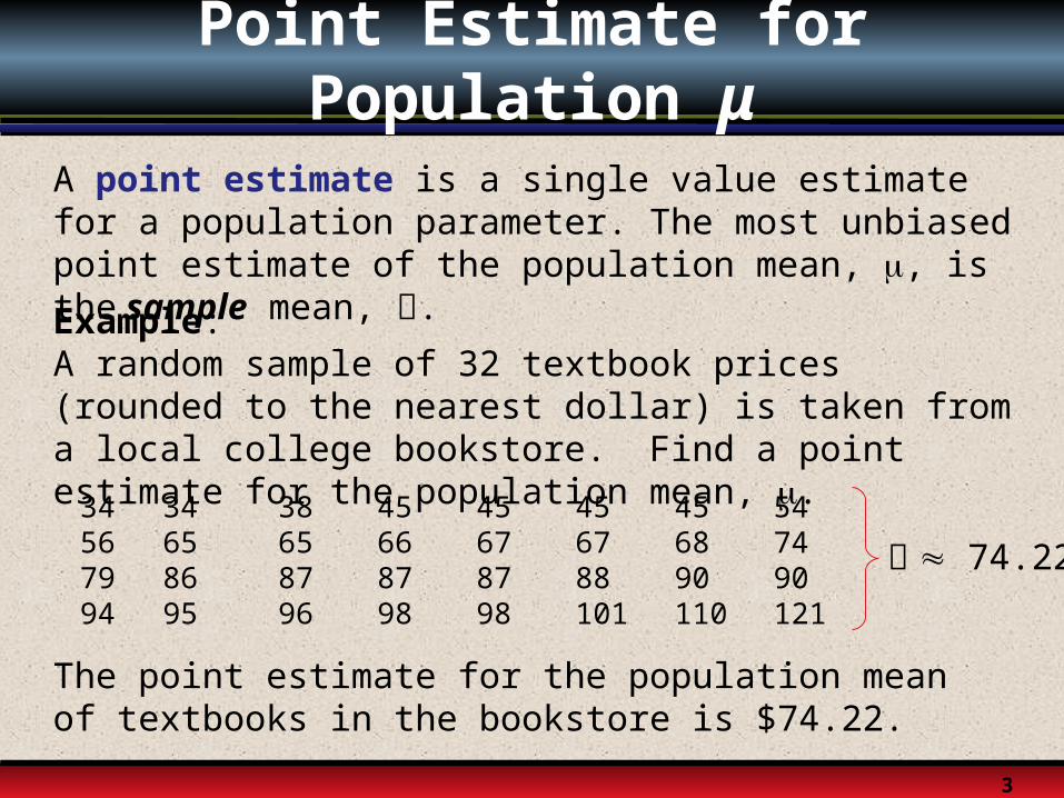
Interval Estimate
An interval estimate is an interval, or range of values, used to estimate a population parameter.
Point estimate for textbooks
• 74.22
interval estimate
How confident do we want to be that the interval estimate contains the population mean, μ?
5
Level of Confidence
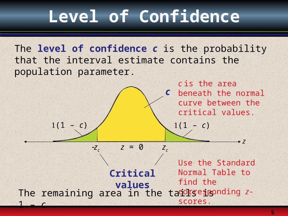
The level of confidence c is the probability that the interval estimate contains the population parameter.
zz = 0zc zc
Critical values
(1 – c) (1 – c)
c is the area beneath the normal curve between the critical values.
The remaining area in the tails is 1 – c .
c
Use the Standard Normal Table to find the corresponding z-scores.
6
Common Levels of Confidence
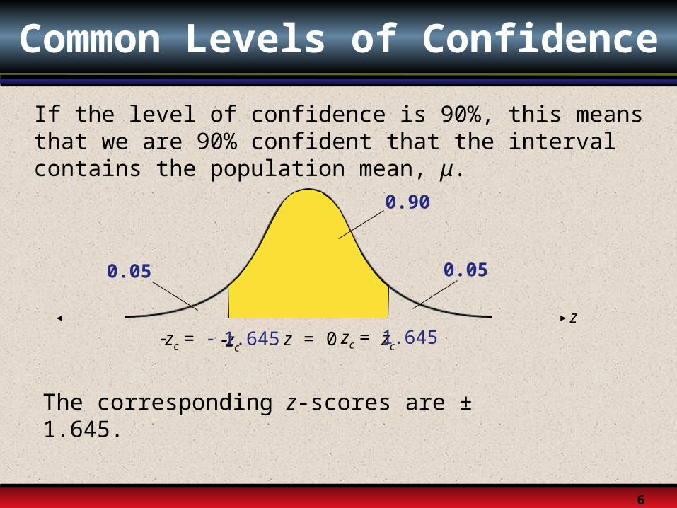
If the level of confidence is 90%, this means that we are 90% confident that the interval contains the population mean, μ.
zz = 0zc zc
The corresponding z-scores are ± 1.645.
0.90
0.050.05
zc = 1.645 zc = 1.645
7
zz = 0zc zc
Common Levels of Confidence
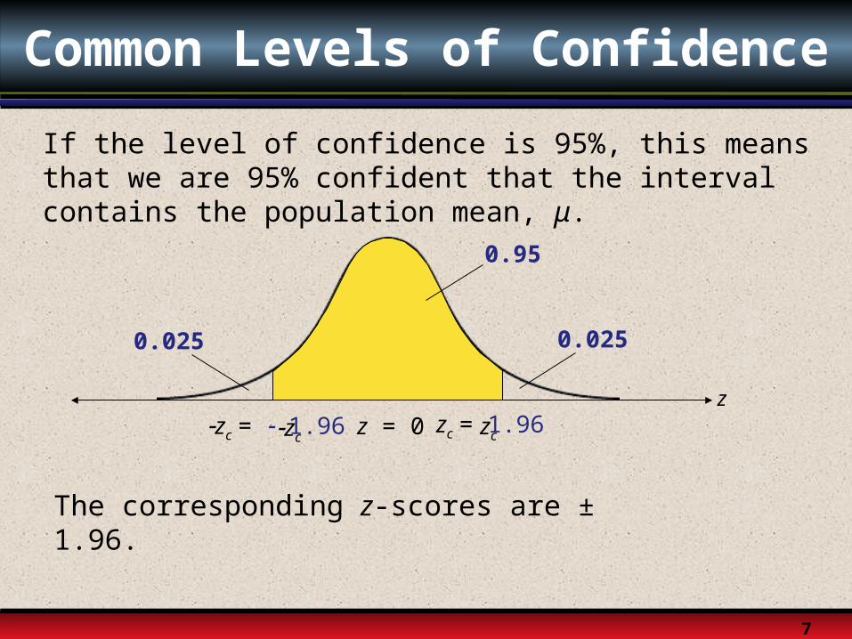
If the level of confidence is 95%, this means that we are 95% confident that the interval contains the population mean, μ.
The corresponding z-scores are ± 1.96.
0.95
0.0250.025
zc = 1.96 zc = 1.96
8
zz = 0zc zc
Common Levels of Confidence
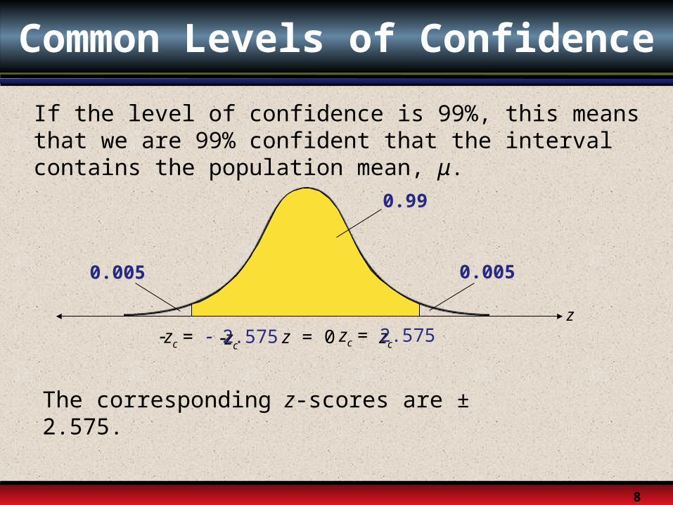
If the level of confidence is 99%, this means that we are 99% confident that the interval contains the population mean, μ.
The corresponding z-scores are ± 2.575.
0.99
0.0050.005
zc = 2.575 zc = 2.575
9
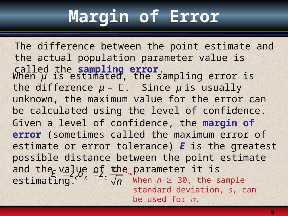
Margin of Error
The difference between the point estimate and the actual population parameter value is called the sampling error. When μ is estimated, the sampling error is the difference μ – . Since μ is usually unknown, the maximum value for the error can be calculated using the level of confidence.Given a level of confidence, the margin of error (sometimes called the maximum error of estimate or error tolerance) E is the greatest possible distance between the point estimate and the value of the parameter it is estimating.
c x cσE z σ zn
When n 30, the sample standard deviation, s, can be used for .
10
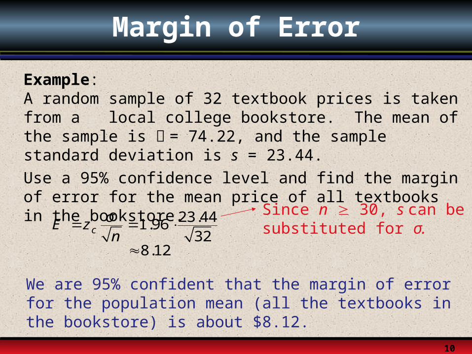
Margin of Error
Example:A random sample of 32 textbook prices is taken from a local college bookstore. The mean of the sample is = 74.22, and the sample standard deviation is s = 23.44. Use a 95% confidence level and find the margin of error for the mean price of all textbooks in the bookstore. 23.441.96
32cσE zn
8.12
We are 95% confident that the margin of error for the population mean (all the textbooks in the bookstore) is about $8.12.
Since n 30, s can be substituted for σ.
11
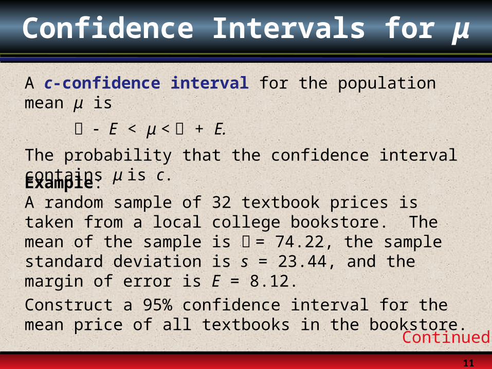
Confidence Intervals for μ
A c-confidence interval for the population mean μ is
E < μ < + E.
The probability that the confidence interval contains μ is c.
Example:A random sample of 32 textbook prices is taken from a local college bookstore. The mean of the sample is = 74.22, the sample standard deviation is s = 23.44, and the margin of error is E = 8.12. Construct a 95% confidence interval for the mean price of all textbooks in the bookstore.
Continued.
12
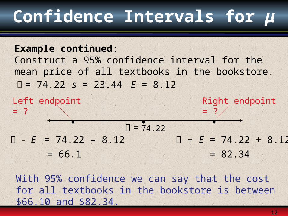
Confidence Intervals for μ
Example continued:Construct a 95% confidence interval for the mean price of all textbooks in the bookstore. = 74.22 s = 23.44 E = 8.12
With 95% confidence we can say that the cost for all textbooks in the bookstore is between $66.10 and $82.34.
• = 74.22 ••
Left endpoint = ? Right endpoint = ?
E = 74.22 – 8.12 + E = 74.22 + 8.12
= 66.1 = 82.34
13
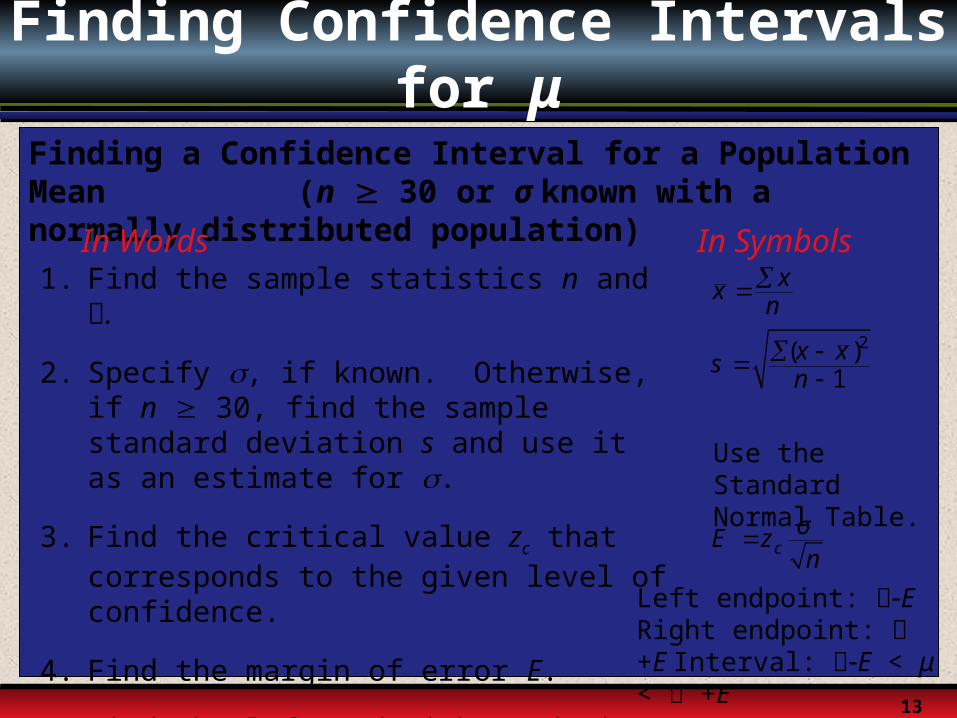
Finding Confidence Intervals for μ
Finding a Confidence Interval for a Population Mean (n 30 or σ known with a normally distributed population)In Words In Symbols1. Find the sample statistics n and .
2. Specify , if known. Otherwise, if n 30, find the sample standard deviation s and use it as an estimate for .
3. Find the critical value zc that corresponds to the given level of confidence.
4. Find the margin of error E.
5. Find the left and right endpoints and form the confidence interval.
n xx
2( )1
sn
x x
Use the Standard Normal Table.
Left endpoint: E Right endpoint: +E Interval: E < μ < +E
cσE zn
14
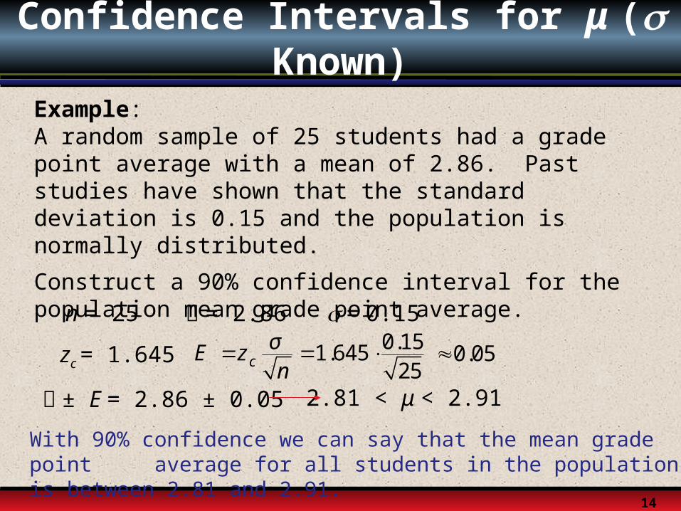
Confidence Intervals for μ ( Known)
Example:A random sample of 25 students had a grade point average with a mean of 2.86. Past studies have shown that the standard deviation is 0.15 and the population is normally distributed.
Construct a 90% confidence interval for the population mean grade point average.
n = 25 = 2.86 = 0.15
zc = 1.645 0.151.64525c
σE zn
± E = 2.86 ± 0.05
0.05
2.81 < μ < 2.91
With 90% confidence we can say that the mean grade point average for all students in the population is between 2.81 and 2.91.
15
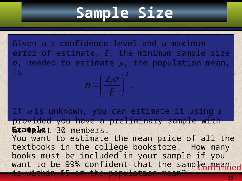
Sample Size
Given a c-confidence level and a maximum error of estimate, E, the minimum sample size n, needed to estimate , the population mean, is
If is unknown, you can estimate it using s provided you have a preliminary sample with at least 30 members.Example: You want to estimate the mean price of all the textbooks in the college bookstore. How many books must be included in your sample if you want to be 99% confident that the sample mean is within $5 of the population mean?
2
.cznE
Continued.
16
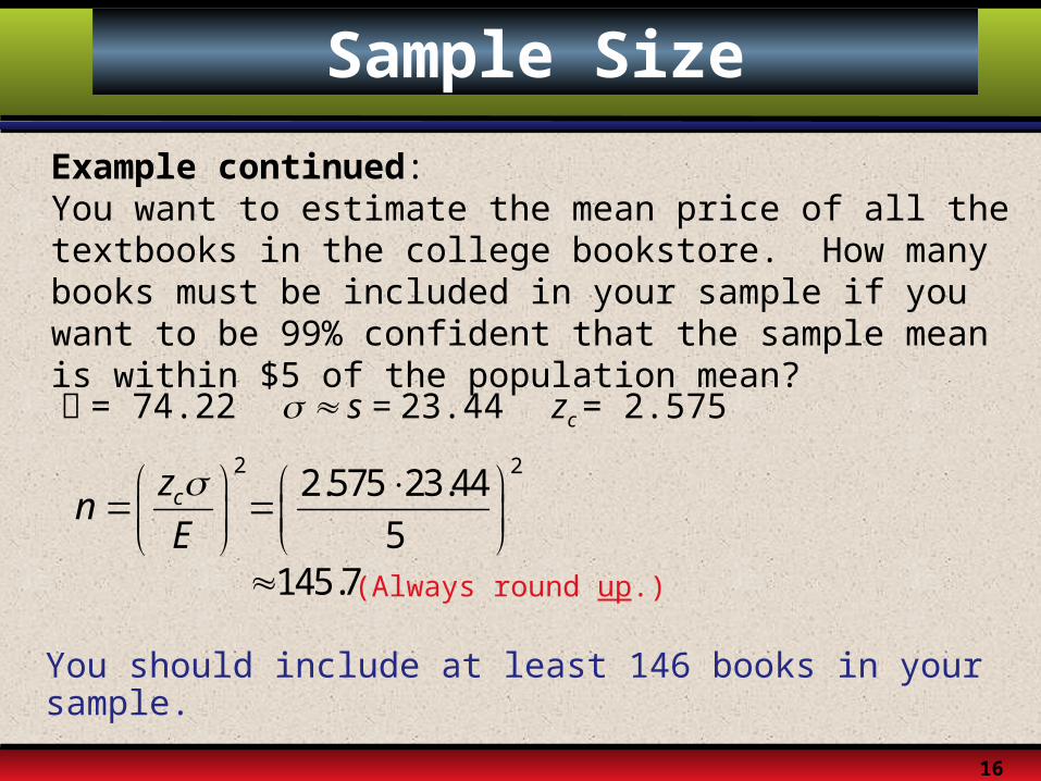
Sample Size
Example continued: You want to estimate the mean price of all the textbooks in the college bookstore. How many books must be included in your sample if you want to be 99% confident that the sample mean is within $5 of the population mean?
2
cznE
= 74.22 s = 23.44 zc = 2.575
22.575 23.44
5
145.7
You should include at least 146 books in your sample.
(Always round up.)
§ 6.2
Confidence Intervals for the Mean (Small
Samples)
18
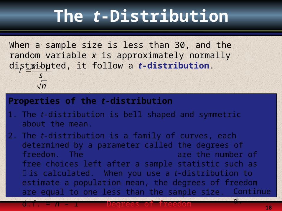
The t-Distribution
Properties of the t-distribution
1. The t-distribution is bell shaped and symmetric about the mean.
2. The t-distribution is a family of curves, each determined by a parameter called the degrees of freedom. The degrees of freedom are the number of free choices left after a sample statistic such as is calculated. When you use a t-distribution to estimate a population mean, the degrees of freedom are equal to one less than the sample size.
d.f. = n – 1 Degrees of freedom
x μtsn
Continued.
When a sample size is less than 30, and the random variable x is approximately normally distributed, it follow a t-distribution.
19
The t-Distribution
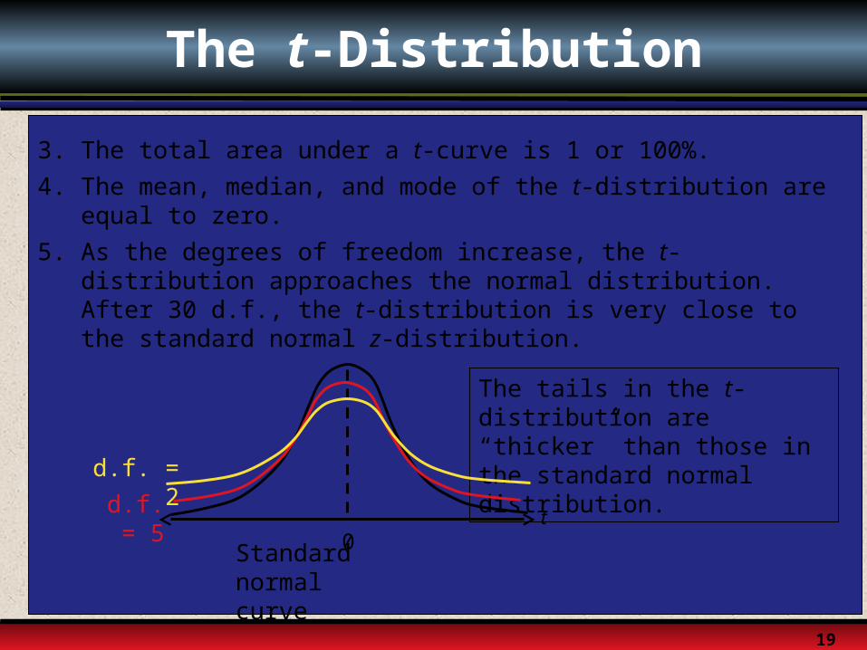
3. The total area under a t-curve is 1 or 100%.
4. The mean, median, and mode of the t-distribution are equal to zero.
5. As the degrees of freedom increase, the t-distribution approaches the normal distribution. After 30 d.f., the t-distribution is very close to the standard normal z-distribution.
t0Standard
normal curve
The tails in the t-distribution are “thicker” than those in the standard normal distribution.
d.f. = 5
d.f. = 2
20
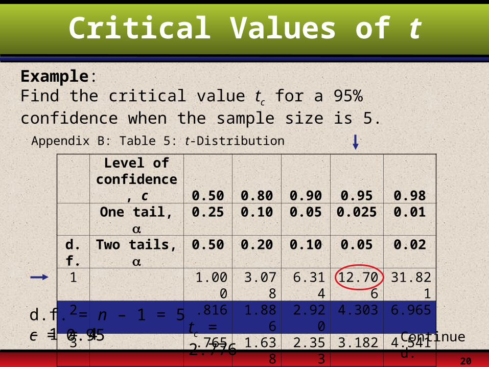
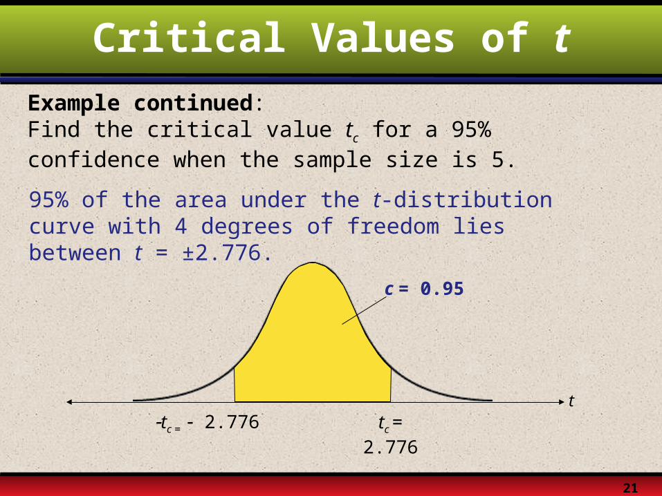
Critical Values of tExample:Find the critical value tc for a 95% confidence when the sample size is 5.
Appendix B: Table 5: t-Distribution
Level of confidence
, c 0.50 0.80 0.90 0.95 0.98One tail, 0.25 0.10 0.05 0.025 0.01
d.f.
Two tails,
0.50 0.20 0.10 0.05 0.02
1 1.000 3.078 6.314 12.706
31.821
2 .816 1.886 2.920 4.303 6.9653 .765 1.638 2.353 3.182 4.5414 .741 1.533 2.132 2.776 3.7475 .727 1.476 2.015 2.571 3.365Continued
.
d.f. = n – 1 = 5 – 1 = 4c = 0.95 tc = 2.776
21
Critical Values of tExample continued:Find the critical value tc for a 95% confidence when the sample size is 5.
95% of the area under the t-distribution curve with 4 degrees of freedom lies between t = ±2.776.
ttc = 2.776 tc =
2.776
c = 0.95

22
Confidence Intervals and t-Distributions
Constructing a Confidence Interval for the Mean: t-Distribution
In Words In Symbols
1. Identify the sample statistics n, , and s.
2. Identify the degrees of freedom, the level of confidence c, and the critical value tc.
3. Find the margin of error E.
4. Find the left and right endpoints and form the confidence interval.
n xx
2( )1
sn
x x
Left endpoint: E Right endpoint: +E Interval: E < μ < +E
csE tn
d.f. = n – 1
23
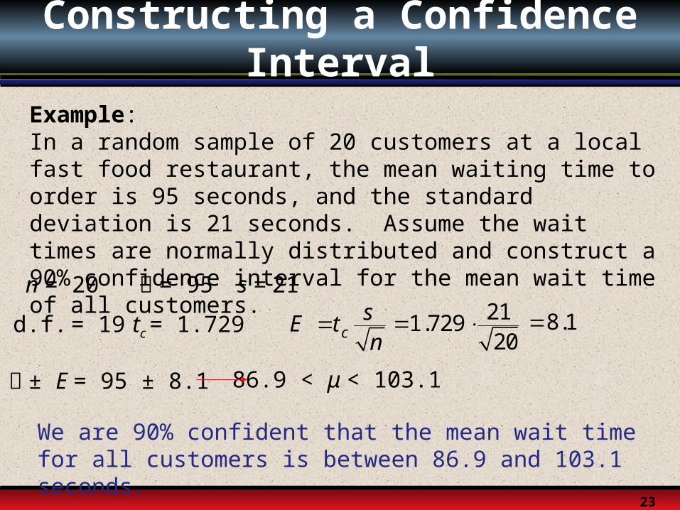
Constructing a Confidence Interval
Example:In a random sample of 20 customers at a local fast food restaurant, the mean waiting time to order is 95 seconds, and the standard deviation is 21 seconds. Assume the wait times are normally distributed and construct a 90% confidence interval for the mean wait time of all customers.
We are 90% confident that the mean wait time for all customers is between 86.9 and 103.1 seconds.
= 95 s = 21
tc = 1.729
n = 20
csE tn
d.f. = 19 211.72920
8.1
± E = 95 ± 8.1 86.9 < μ < 103.1
24
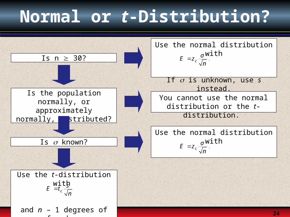
Normal or t-Distribution?
Is n 30?
Is the population normally, or approximately normally,
distributed?
You cannot use the normal distribution or the t-distribution.
No
Yes
Is known?
No
Use the normal distribution with
If is unknown, use s instead.
.cσE zn
Yes
No
Use the normal distribution with
.cσE zn
Yes
Use the t-distribution with
and n – 1 degrees of freedom.
csE tn
25
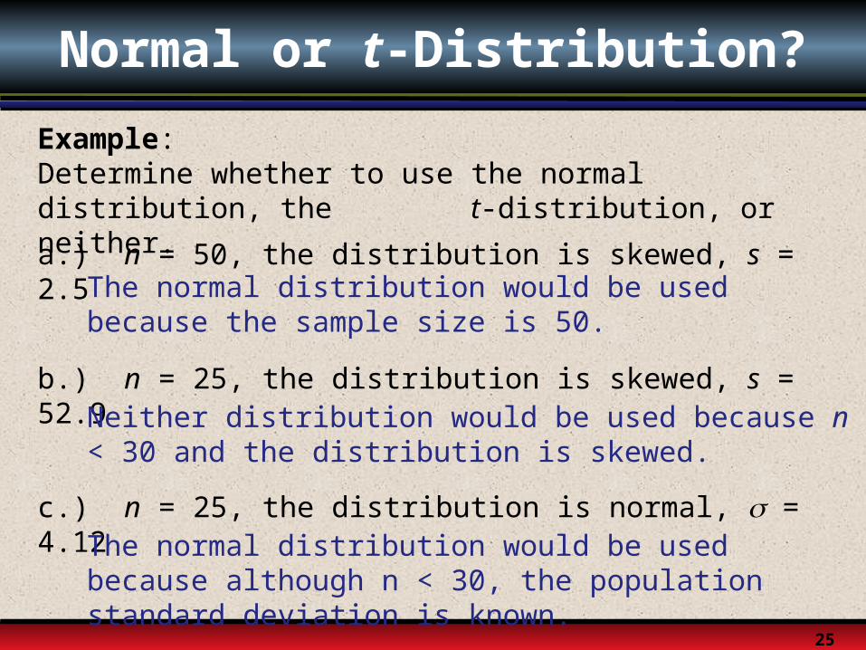
Normal or t-Distribution?
Example:Determine whether to use the normal distribution, the t-distribution, or neither.
a.) n = 50, the distribution is skewed, s = 2.5The normal distribution would be used because the sample size is 50.
b.) n = 25, the distribution is skewed, s = 52.9Neither distribution would be used because n < 30 and the distribution is skewed.
c.) n = 25, the distribution is normal, = 4.12The normal distribution would be used because although n < 30, the population standard deviation is known.
§ 6.3
Confidence Intervals for Population Proportions
27
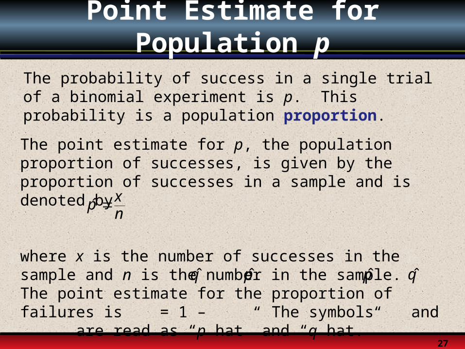
Point Estimate for Population p
The probability of success in a single trial of a binomial experiment is p. This probability is a population proportion.
The point estimate for p, the population proportion of successes, is given by the proportion of successes in a sample and is denoted by
where x is the number of successes in the sample and n is the number in the sample. The point estimate for the proportion of failures is = 1 – The symbols and are read as “p hat” and “q hat.”
ˆ xpn
q̂ .̂p q̂p̂
28
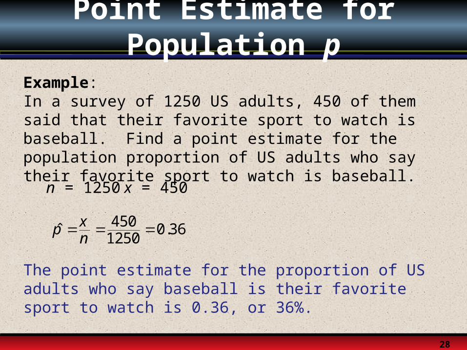
Point Estimate for Population p
Example:In a survey of 1250 US adults, 450 of them said that their favorite sport to watch is baseball. Find a point estimate for the population proportion of US adults who say their favorite sport to watch is baseball.
The point estimate for the proportion of US adults who say baseball is their favorite sport to watch is 0.36, or 36%.
450 0.36ˆ 1250xpn
n = 1250 x = 450
29
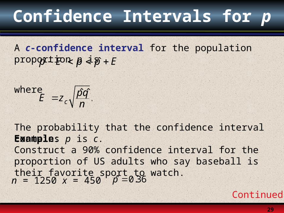
Confidence Intervals for p
A c-confidence interval for the population proportion p is
where
The probability that the confidence interval contains p is c.Example:Construct a 90% confidence interval for the proportion of US adults who say baseball is their favorite sport to watch.
Continued.
ˆ ˆp E p p E
ˆ .̂cpqE zn
0.36p̂ n = 1250 x = 450
30
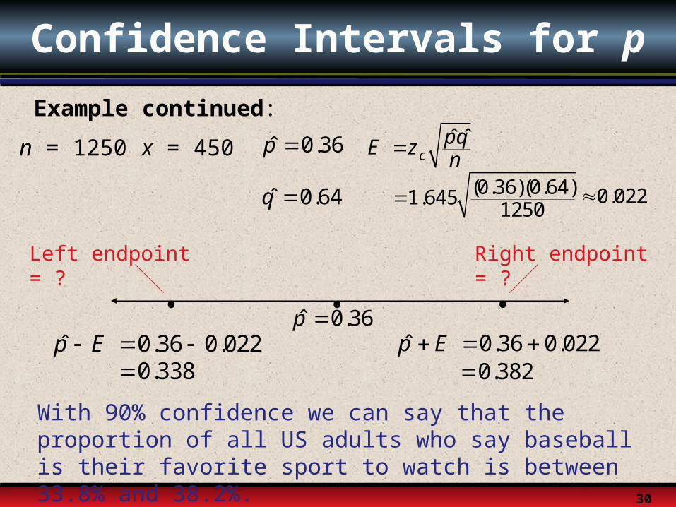
Confidence Intervals for p
0.36 0.022p̂ E
Example continued:
With 90% confidence we can say that the proportion of all US adults who say baseball is their favorite sport to watch is between 33.8% and 38.2%.
Left endpoint = ? Right endpoint = ?
0.36p̂ n = 1250 x = 450
• •• 0.36p̂
ˆ ˆc
pqE zn
(0.36)(0.64)1.6451250
0.64q̂
0.36 0.022p̂ E
0.022
0.338 0.382
31
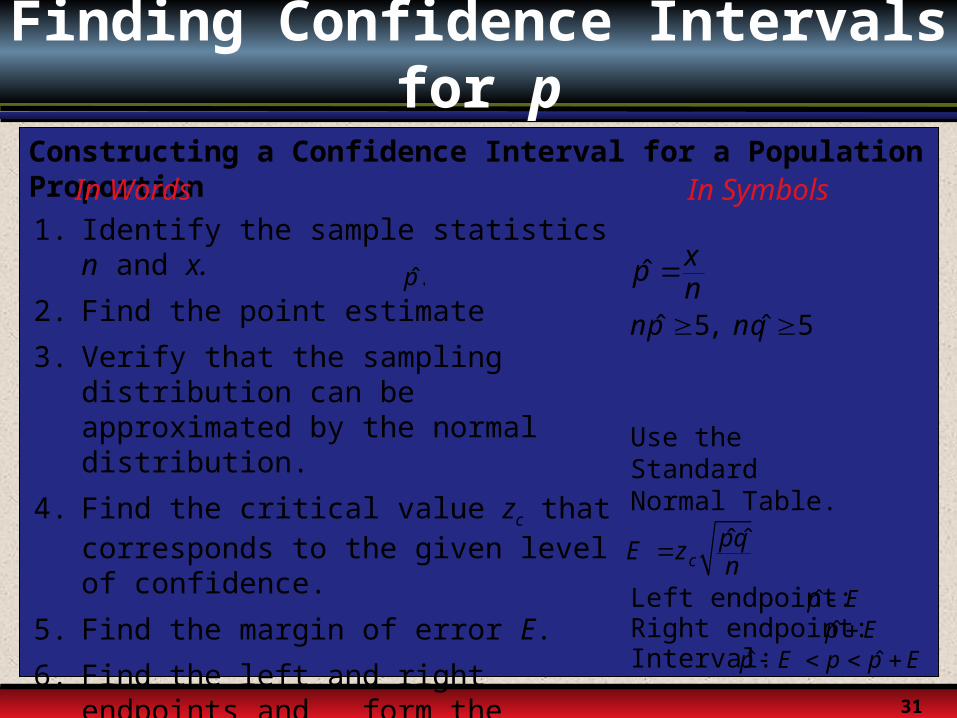
Finding Confidence Intervals for p
Constructing a Confidence Interval for a Population ProportionIn Words In Symbols1. Identify the sample statistics n and
x.
2. Find the point estimate
3. Verify that the sampling distribution can be approximated by the normal distribution.
4. Find the critical value zc that corresponds to the given level of confidence.
5. Find the margin of error E.
6. Find the left and right endpoints and form the confidence interval.
ˆ xpn
Use the Standard Normal Table.
ˆ ˆc
pqE zn
.̂p
5, 5ˆ ˆnp nq
Left endpoint: Right endpoint: Interval:
p̂ Ep̂ E
ˆ ˆp E p p E
32
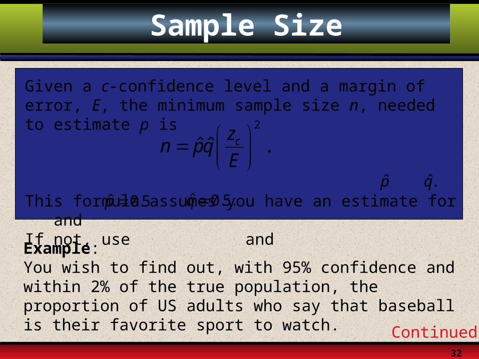
Sample Size
Given a c-confidence level and a margin of error, E, the minimum sample size n, needed to estimate p is
This formula assumes you have an estimate for and If not, use and
Example: You wish to find out, with 95% confidence and within 2% of the true population, the proportion of US adults who say that baseball is their favorite sport to watch.
2
ˆ ˆ .
czn pqE
Continued.
ˆ.qp̂ˆ 0.5.qˆ 0.5p
33
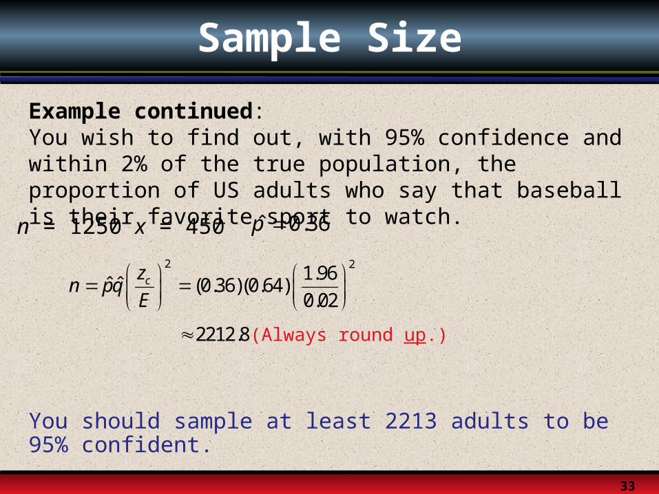
Sample Size
You should sample at least 2213 adults to be 95% confident.
(Always round up.)
Example continued: You wish to find out, with 95% confidence and within 2% of the true population, the proportion of US adults who say that baseball is their favorite sport to watch.
0.36p̂ n = 1250 x = 450
2 21.96
ˆ ˆ (0.36)(0.64)0.02
czn pqE
2212.8

§ 6.4
Confidence Intervals for Variance and
Standard Deviation
35
The Chi-Square Distribution
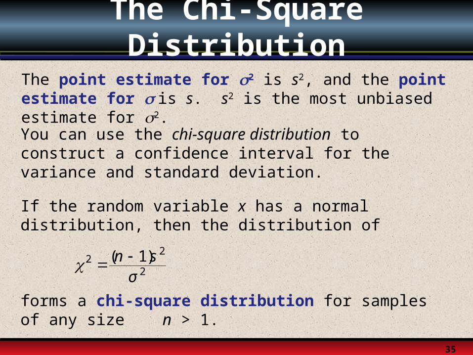
The point estimate for 2 is s2, and the point estimate for is s. s2 is the most unbiased estimate for 2. You can use the chi-square distribution to construct a confidence interval for the variance and standard deviation.
If the random variable x has a normal distribution, then the distribution of
forms a chi-square distribution for samples of any size n > 1.
22
2( 1)n s
σ
36
The Chi-Square Distribution
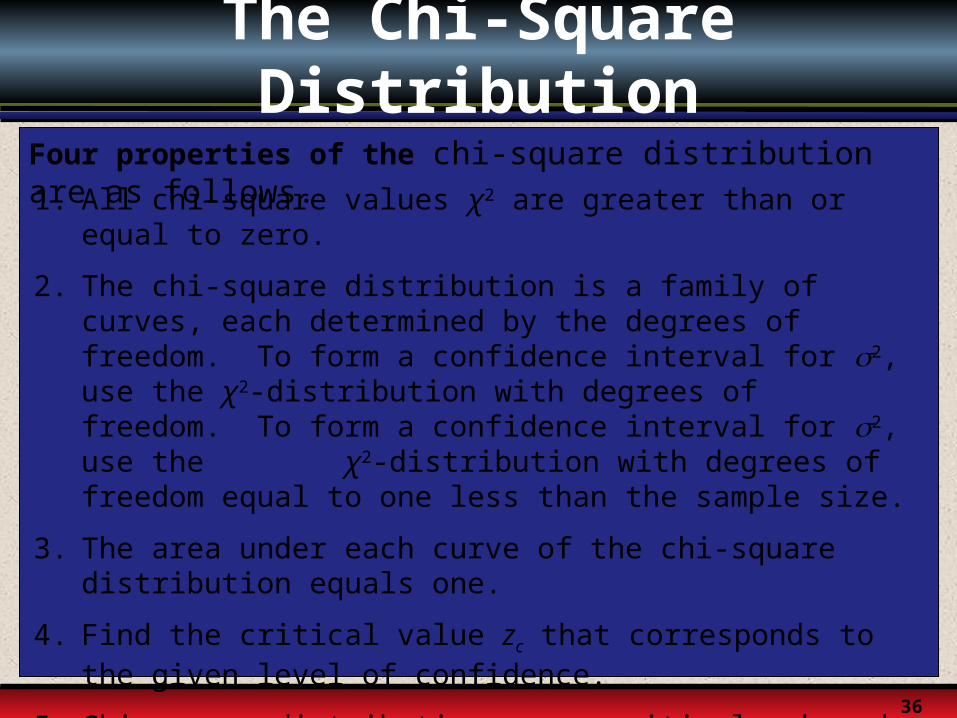
Four properties of the chi-square distribution are as follows.1. All chi-square values χ2 are greater than or equal to
zero.
2. The chi-square distribution is a family of curves, each determined by the degrees of freedom. To form a confidence interval for 2, use the χ2-distribution with degrees of freedom. To form a confidence interval for 2, use the χ2-distribution with degrees of freedom equal to one less than the sample size.
3. The area under each curve of the chi-square distribution equals one.
4. Find the critical value zc that corresponds to the given level of confidence.
5. Chi-square distributions are positively skewed.
37
Critical Values for X2
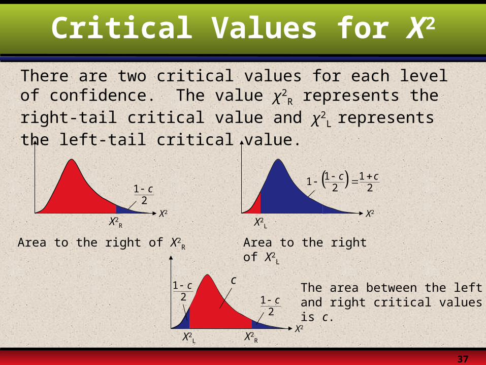
There are two critical values for each level of confidence. The value χ2
R represents the right-tail critical value and χ2
L represents the left-tail critical value.
X2
12
c
X2R
Area to the right of X2R
X2
1 112 2
c c
X2L
Area to the right of X2
L
The area between the left and right critical values is c.
X2
X2RX2
L
c12
c1
2c
38
Critical Values for X2
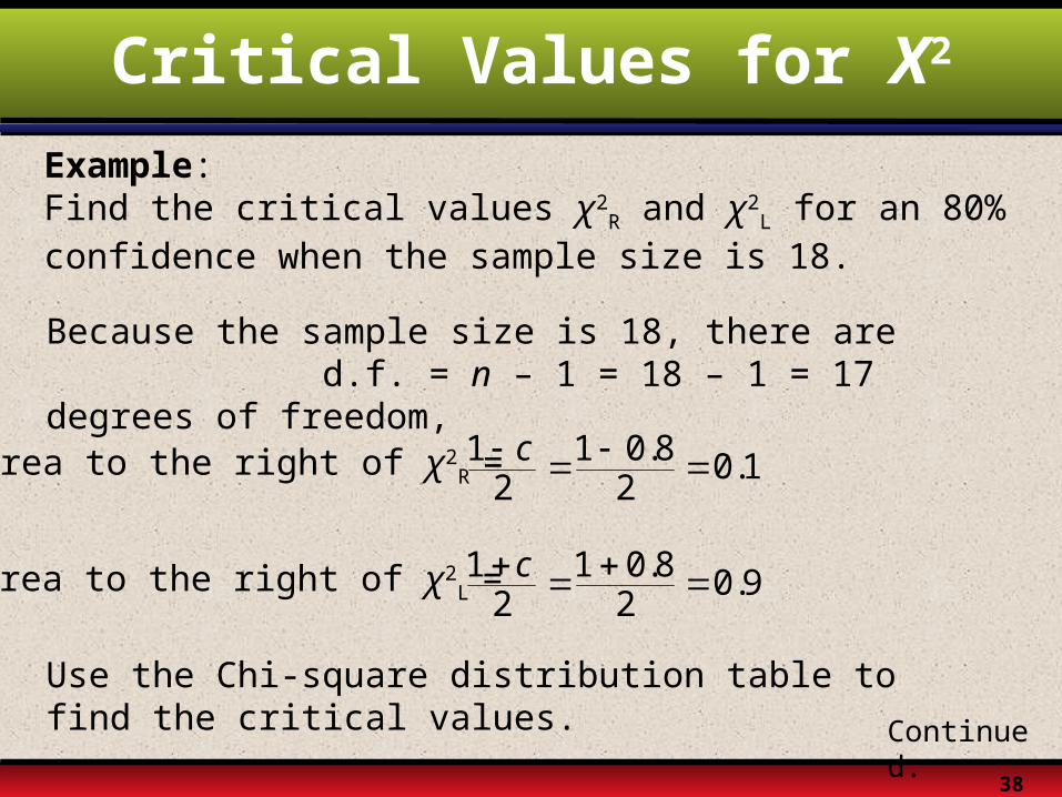
Example:Find the critical values χ2
R and χ2L for an 80%
confidence when the sample size is 18.
Continued.
Because the sample size is 18, there are d.f. = n – 1 = 18 – 1 = 17 degrees of freedom,
Area to the right of χ2R = 1 1 0.8 0.1
2 2c
Area to the right of χ2L = 1 1 0.8 0.9
2 2c
Use the Chi-square distribution table to find the critical values.
39
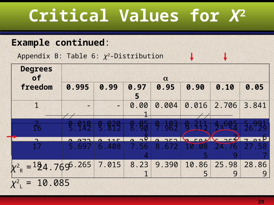
Critical Values for X2
Example continued:
Appendix B: Table 6: χ2-Distribution
Degrees of
freedom 0.995 0.99 0.975
0.95 0.90 0.10 0.05
1 - - 0.001 0.004 0.016 2.706 3.8412 0.010 0.020 0.051 0.103 0.211 4.605 5.9913 0.072 0.115 0.216 0.352 0.584 6.251 7.81516 5.142 5.812 6.908 7.962 9.312 23.54
226.29
617 5.697 6.408 7.564 8.672 10.08
524.76
927.58
718 6.265 7.015 8.231 9.390 10.86
525.98
928.86
9χ2
R = 24.769
χ2L = 10.085
40
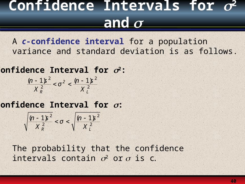
Confidence Intervals for 2 and
A c-confidence interval for a population variance and standard deviation is as follows.
The probability that the confidence intervals contain 2 or is c.
2 2
2 2( 1) ( 1)2
R L
n s n sσX X
Confidence Interval for 2:
2 2
2 2( 1) ( 1)
R L
n s n sσX X
Confidence Interval for :
41
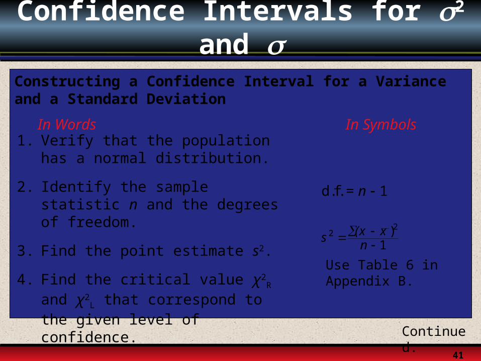
Confidence Intervals for 2 and
Constructing a Confidence Interval for a Variance and a Standard Deviation
In Words In Symbols1. Verify that the population has a
normal distribution.
2. Identify the sample statistic n and the degrees of freedom.
3. Find the point estimate s2.
4. Find the critical value χ2R and χ2
L that correspond to the given level of confidence.
Use Table 6 in Appendix B.
22 )
1(x xsn
d.f. = 1n
Continued.
42
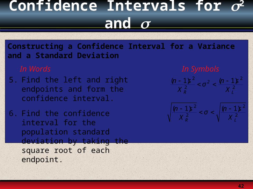
Confidence Intervals for 2 and
Constructing a Confidence Interval for a Variance and a Standard Deviation
In Words In Symbols5. Find the left and right
endpoints and form the confidence interval.
6. Find the confidence interval for the population standard deviation by taking the square root of each endpoint.
2 2
2 2( 1) ( 1)2
R L
n s n sσX X
2 2
2 2( 1) ( 1)
R L
n s n sσX X
43
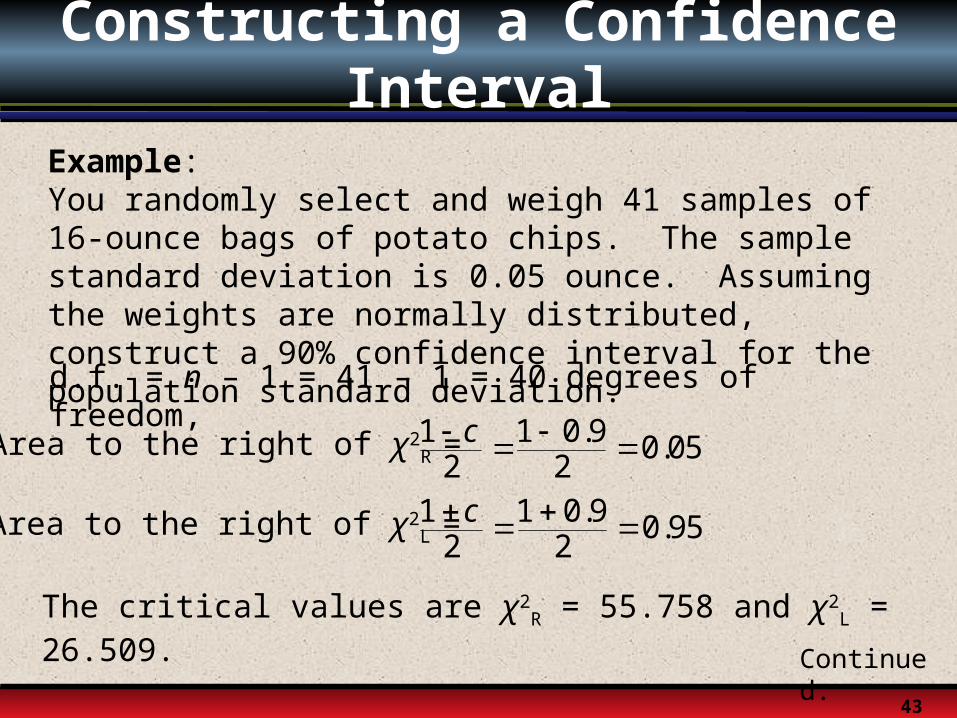
Constructing a Confidence Interval
Example:You randomly select and weigh 41 samples of 16-ounce bags of potato chips. The sample standard deviation is 0.05 ounce. Assuming the weights are normally distributed, construct a 90% confidence interval for the population standard deviation.
d.f. = n – 1 = 41 – 1 = 40 degrees of freedom,
Area to the right of χ2R = 1 1 0.9 0.05
2 2c
Area to the right of χ2L = 1 1 0.9 0.95
2 2c
The critical values are χ2R = 55.758 and χ2
L = 26.509.
Continued.
44
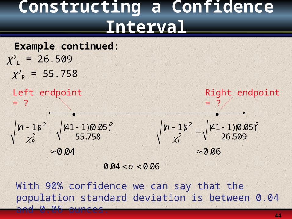
Constructing a Confidence Interval
Example continued:
χ2R = 55.758
χ2L = 26.509
2 2
2( 1) (41 1)(0.05)
55.758R
n s
With 90% confidence we can say that the population standard deviation is between 0.04 and 0.06 ounces.
Left endpoint = ? Right endpoint = ?
••2 2
2( 1) (41 1)(0.05)
26.509L
n s
0.04 0.06
0.04 0.06σ