Chapter 7, Part One

Confidence Intervals for

Population Proportions

Population vs. Sample(Review from Chapter 1)

• Population: The set of ALL individuals we

are interested in studying.

• Sample: The set of individuals for which

we have actual data.

• Statistical Inference: Using information

from a given Sample to draw conclusions

about the entire Population.

Parameters vs. Statistics(Review from Chapter 1)

• The goal of statistical inference is to use sample data to draw conclusions about some VERY LARGE population.

• A parameter is a numerical value describing some aspect of the population.

• A statistic is a numerical value describing some aspect of a sample.

• The value of a statistic (computed from sample data) is often used to estimate the value of a parameter (which is usually unknown).

Basic Requirements

• We typically require that our sample data comes from a Simple Random Sample of size n. (all groups of the given size are equally likely to be the sample)

• Additional requirements depend on the parameter in question.

• Pay attention to these requirements—if they are not satisfied, your conclusions may be invalid!

Population Demographics

• The Pew Research Center estimates the

following based on results of a May 2013 phone

poll of 1,895 adult American internet users:

– 72% of American internet users use some kind of

social networking site.

– 74% of female American internet users use some

kind of social networking site.

– 70% of male American internet users use some kind

of social networking site.

• These are statistics (from sample data).

Point Estimate

• What we really want to know: what percent of ALL American internet users use some kind of social networking site?

– This is a parameter: a number (with unknown value) describing some large population.

• The value of a statistic (known) can be used to estimate of the value of a parameter (unknown). Without additional information, this is called a point estimate.

• The main problem: A point estimate provides no indication of how “good” the estimate might be.

Confidence Intervals

• More useful is a Confidence Interval: a claim that our (unknown) value is in a certain range.

• In practice, this is most often reported as:1. Value of some statistic (What is the estimate?)

2. Margin of Error (How close is our estimate to the true value?)

3. Confidence Level (What is the probability that we’re correct?)

• Example: The percent of adult American internet users who use social media is 72% ± 2.5%, with a confidence level of 95%.

• Note: NOBODY KNOWS if this claim is actually correct (why not?)

Population Proportions: Notation

• Our parameter: What proportion of the population satisfies a given condition?– An individual satisfying the condition is often called a

“success,” regardless of context.

• 𝑝 = proportion of “successes” in the entire population. This value is UNKNOWN.

• 𝑝 = proportion of “successes” in the sample. This value is computed from actual data.

• 𝑞 = 1 − 𝑝 is the proportion of “failures” in the sample (individuals that fail to satisfy the given condition).

Population Proportions:

Requirements

• We can safely assume that (for all samples of size n) 𝑝 has an approximately Normal distribution, provided that:

• Our sample is an SRS of size n.

• The sample contains at least 5 “successes” and at least 5 “failures.”

• Note: If you are not told the number of successes/failures, check that both:

• 𝑝𝑛 ≥ 5

• 𝑞𝑛 ≥ 5

Population Proportions:

Sampling Distribution

Under the conditions on the previous slide, 𝑝(for all samples of size n) has a roughly Normal distribution, with:

• (Mean of 𝑝) = p

• (Std. Dev. of 𝑝) = 𝑝𝑞/𝑛 = 𝑝 (1 − 𝑝)/𝑛

Since we don’t know the value of p, we can approximate Std. Dev. by using:

𝑝 𝑞/𝑛 = 𝑝(1 − 𝑝)/𝑛

This is called the Standard Error of 𝑝.

Example: Polling Data

In the Pew Research poll, let p be the

proportion of internet users who use some

kind of social networking site. We had:

• Sample size: n = 1895.

• Percentage who use social networking:

72% (most likely, this was rounded).

• 𝑝 = 0.72 (converted to a proportion).

• 𝑞 = 1 − 0.72 = 0.28

Example: Polling Data

Since the number of “successes” and

“failures” is not reported in the data, we

need to compute:

• 𝑝𝑛 = (.72) x (1895) = 1364.4.

• 𝑞𝑛 = (.28) x (1895) = 530.6

Both numbers are at least 5, so this

requirement is satisfied.

Example: Polling Data

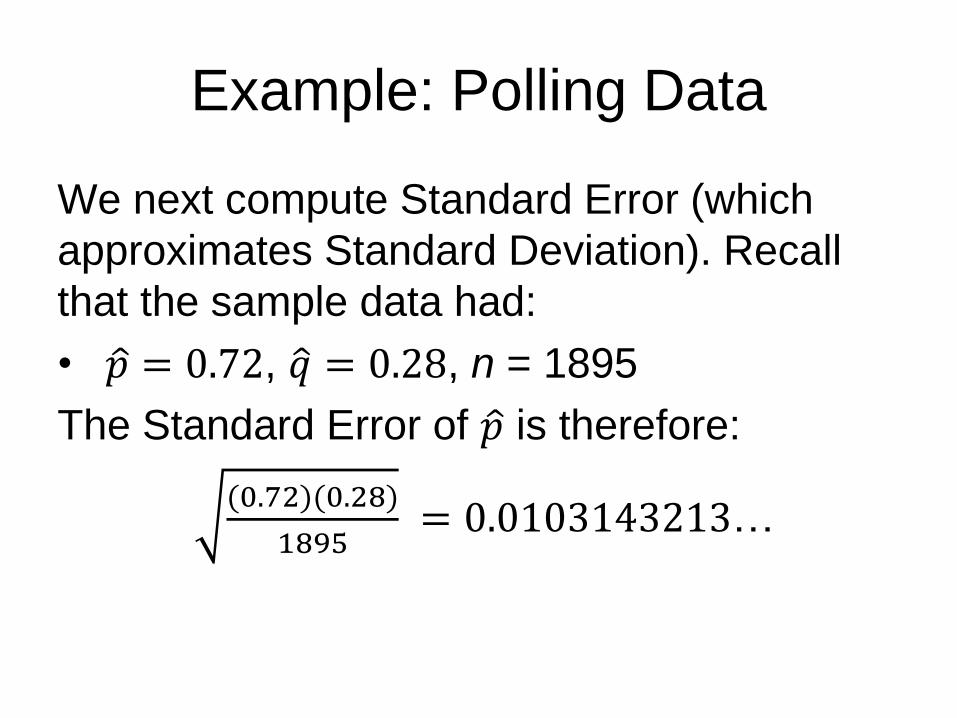
We next compute Standard Error (which

approximates Standard Deviation). Recall

that the sample data had:

• 𝑝 = 0.72, 𝑞 = 0.28, n = 1895

The Standard Error of 𝑝 is therefore:

(0.72)(0.28)

1895= 0.0103143213…

Summary thus far

We can assume that for all samples of the

given size (n = 1895)…

• 𝑝 has an approx. Normal distribution.

• (Mean of 𝑝) = p [this value is unknown]

• (Std. Dev. of 𝑝) is approximately 0.01031

Fill in the blank: 95% of all samples (of size

1895) would have 𝑝 within ____ of p.

A Confidence Interval

• Question: 95% of all samples (of size

1895) would have 𝑝 in what range?

• Answer: Within two Std. Dev. of the

mean. From work above, about 0.02062.

• If we assume an SRS, there is a 95%

chance that the 𝑝 from the sample (0.72)

is within (0.02062) of the [unknown] true

value of the population proportion, p.

A Confidence Interval

• Based on the polling data, we claim:

(0.72)-(0.02062) < p < (0.72)+(0.02062)

• These are proportions. As percents, the

above range is: 69.938% - 74.062%

• Is the actual value of p in the given

range? NOBODY KNOWS.

• But WE DO KNOW the probability that

our claim is correct: 95% in this case.

Confidence Intervals

• A Confidence Interval is a claim that the [unknown] value of some parameter is within a given range of values.

• This range is computed from sample data. Different samples give different ranges!!

• WE WILL NEVER KNOW if our claim is correct, but we do know the probabilitythat it is correct. This probability is called the confidence level.

Margin of Error

• Most real-world applications report a confidence interval in the form:

(Point Estimate) ± (Margin of Error)

• The Point Estimate is a Sample Statistic, computed from sample data.• Example: 72% of internet users use some kind of

social networking site.

• Margin of Error indicates how accurate the Point Estimate is likely to be.• Example: We computed a 2.062% MoE above. Pew

reported 2.5% (the discrepancy is because Pew used more realistic sampling methods, not an SRS).

Confidence Level

• A Confidence Interval is a claim that the

value of some parameter is within a

certain range of values.

• The Confidence Level is the probability

that this claim is correct.

• 95% is a VERY COMMON choice.

A General Template(This is EXTREMELY USEFUL, but not in the textbook!)

• Every confidence interval in this course has the same basic form:

(Sample Statistic) ± (Margin of Error)

• Sample Statistic is often computed for you.

• Margin of Error will have the form:

(Critical Value)x(Std. Dev. OR Std. Error)

• Critical Value: Depends only on the Confidence Level. Computed using a table.

• Standard Deviation/Error: Computed by you from an appropriate formula.

MoE for Population Proportion

• When estimating a population proportion

𝑝, we use the Standard Error of 𝑝 :

𝑝 𝑞/𝑛 = 𝑝(1 − 𝑝)/𝑛

• The Critical Value is based on the

Standard Normal distribution (z-scores).

• Once you are told what Confidence Level

to use, there are several ways to compute

the Critical Value.

Critical Values: Table A-2

• For Critical Values based on z-scores:

• Write the confidence level in decimal form,

and let α = 1 – (Confidence Level).

• Using Table A-2, find the cutoff z-score for a

proportion of α/2. This z will be negative.

• The critical value is the z-score from the

previous step, without the negative sign.

• The text calls this value 𝑧𝛼/2, and uses a

more complicated method to find it.

Example: 95% Confidence Level

• Decimal form: Confidence Level = 0.95

• α = 1 – 0.95 = 0.05

• α/2 = 0.025

• Table A-2: The proportion .0250 is in the

table! This gives z = -1.96.

• (Critical value for 95%) = 1.96.

• Note: This is more accurate than “within 2

std. deviations” using the 68-95-99.7 rule.

Common Critical Values

• Confidence levels of 90%, 95%, or 99%

are commonly used. Your z-score table

(A-2) lists their critical values directly:

• 90%: Critical z-Value = 1.645

• 95%: Critical z-Value = 1.960

• 99%: Critical z-Value = 2.575

Critical Values: Table A-3

For Confidence Levels of 80%, 90%, 95%,

98%, and 99%, there is an easier way to find

the Critical Value, using Table A-3:

• Write the confidence level in decimal form,

and let α = 1 – (Confidence Level).

• In “Area in Two Tails,” find the column whose

heading is the value of α.

• For Critical Values based on z-scores, use

the “Large” row at the bottom of the table.

Example: Affordable Care Act

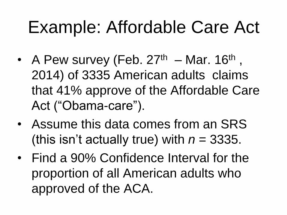
• A Pew survey (Feb. 27th – Mar. 16th ,

2014) of 3335 American adults claims

that 41% approve of the Affordable Care

Act (“Obama-care”).

• Assume this data comes from an SRS

(this isn’t actually true) with n = 3335.

• Find a 90% Confidence Interval for the

proportion of all American adults who

approved of the ACA.

Example: Affordable Care Act

• From the data: 𝑝 = 41% = 0.41

• Compute 𝑞 = 1 − 0.41 = 0.59.

• 𝑛 𝑝 = 1367, 𝑛 𝑞 = 1968; requirements OK.

• The Standard Error of 𝑝 is:

𝑝 𝑞/𝑛 = 0.41 ∗ 0.59/3335 = 0.008516…

• Critical Value (90% level): z = 1.645.

• MoE: (0.008517)*(1.645) = .014 = 1.4%

Example: Affordable Care Act

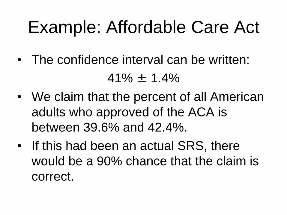
• The confidence interval can be written:

41% ± 1.4%

• We claim that the percent of all American

adults who approved of the ACA is

between 39.6% and 42.4%.

• If this had been an actual SRS, there

would be a 90% chance that the claim is

correct.

Additional Examples

• Use the same data ( 𝑝 = 0.41, n = 3335,

assuming an SRS) to construct:

• An 80% confidence interval for p.

• A 98% confidence interval for p.

• A 99% confidence interval for p.

• Use your previous work, when possible.

• Compare the Margin of Error for each

confidence interval. What do you see?