Chapter 7: Model Grid Setup 7 Map Projection, Model … Map Projection, Model Grid Setup and Grid...

Chapter 7: Model Grid Setup

CAPS - ARPS Version 4.0 192

7 Map Projection, ModelGrid Setup and GridNesting

7.1. Introduction ___________________________________________

This chapter describes the map projection options, the setup of thecomputational grid (including the options for vertical grid stretching), theadaptive grid refinement and grid nesting capability, and the model domaintranslation capabilities.

7.2. Map Projection ________________________________________

ARPS includes a set of map projection subroutines which transformthe Cartesian computational coordinates to latitude and longitude locations onthe Earth and vice versa. Three different map projections are currentlysupported. The map projection factors are not included in the dynamicequations of ARPS version 4.0, but will be in a future release. They are,however, already included in the pre- and post-processors. If one chooses theLambert conformal projection and uses a relatively small model domain (lessthan 1000 km), then the effect of the map factor is negligible.

7.2.1. Map projection options

The three map projection options available in ARPS include 1) polarstereographic, which is most useful at high latitudes and for interfacing withmany large-scale NWP models, 2) Lambert conformal, most useful at mid-latitudes, and 3) Mercator, which is best for low latitudes, generally within 20degrees of the equator. Because some archived data are provided on latitude-longitude grids, a latitude-longitude coordinate option is also provided as part



of the map projection utilities, but, because it is non-conformal, it is notrecommended for use as a model coordinate.

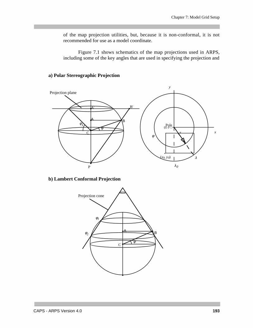
Figure 7.1 shows schematics of the map projections used in ARPS,including some of the key angles that are used in specifying the projection and

a) Polar Stereographic Projection

λ0

λ

φ

Pole

r

y

x

•

•

•(0, 0 )

(x0, y0)

φφ1

Α Β

A' B'

P

C

Projection plane

b) Lambert Conformal Projection

φ

φ1

Α Β

C

φ2

Projection cone



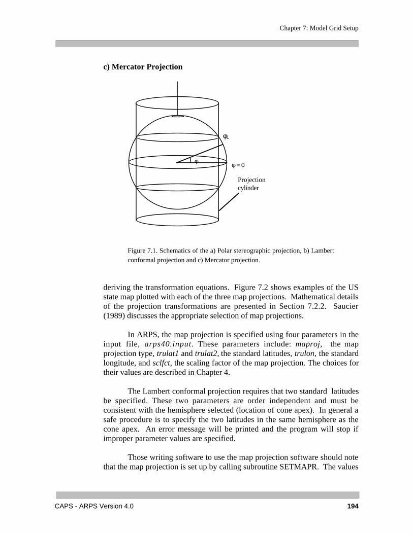
c) Mercator Projection

φ = 0φ

Projectioncylinder

φ1

Figure 7.1. Schematics of the a) Polar stereographic projection, b) Lambert

conformal projection and c) Mercator projection.

deriving the transformation equations. Figure 7.2 shows examples of the USstate map plotted with each of the three map projections. Mathematical detailsof the projection transformations are presented in Section 7.2.2. Saucier(1989) discusses the appropriate selection of map projections.

In ARPS, the map projection is specified using four parameters in theinput file, arps40.input. These parameters include: maproj, the mapprojection type, trulat1 and trulat2, the standard latitudes, trulon, the standardlongitude, and sclfct, the scaling factor of the map projection. The choices fortheir values are described in Chapter 4.

The Lambert conformal projection requires that two standard latitudesbe specified. These two parameters are order independent and must beconsistent with the hemisphere selected (location of cone apex). In general asafe procedure is to specify the two latitudes in the same hemisphere as thecone apex. An error message will be printed and the program will stop ifimproper parameter values are specified.

Those writing software to use the map projection software should notethat the map projection is set up by calling subroutine SETMAPR. The values



of the map projection parameters being used can be retrieved by callingsubroutine GETMAPR. Only one map projection can be active at a time.

Figure 7.2. Examples of US political boundaries plotted with a) Polar

stereographic, b) Lambert conformal and c) Mercator projections.



7.2.2. Map transformations

Transformation equations are used to map the earth coordinates to theprojection plane. This section describes the transformation equations and themagnification of distances from the earth’s surface to the map projectionsurface for each of the map projections. All three primary map projections areconformal, that is the projection magnification, known as the image scale, isthe same in all directions.

a) Polar stereographic projection

The polar stereographic projection is created by projection raysbeginning at the opposite pole and running through each point on the earth’ssurface to the projection plane, which is a plane parallel to the equator at thelatitude specified by the input parameter trulat1, φ1, as illustrated in Fig. 7.1a.

Considering the earth angles as projected on the plane (see Fig. 7.1b),the transformation equation from earth to map coordinates is

x = r sin λ − λ0( )y = −r cos λ − λ0( ) (7.2.1)

r = σre cosφ

where λ is the longitude, φ is the latitude, and re is the radius of the earth.

The variable λ0 is the input parameter trulon. That meridian defines the ycoordinate on the plane. Unless one is trying to match the orientation of anexternal data grid, a λ near the center of the grid should be specified as λο .

The polar stereographic image scale, σ in Eq. (7.2.1), can be derivedfrom the geometry of the triangles in Fig 7.1a and is written

σ = 1 + sin φ1

1 + sin φ. (7.2.2)

Clearly φ1, the input parameter trulat1, should be near the grid center to keep

σ near unity. The input parameter named trulat2 is not used in this projection.



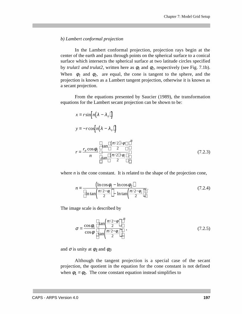
b) Lambert conformal projection

In the Lambert conformal projection, projection rays begin at thecenter of the earth and pass through points on the spherical surface to a conicalsurface which intersects the spherical surface at two latitude circles specifiedby trulat1 and trulat2, written here as φ1 and φ2, respectively (see Fig. 7.1b).

When φ1 and φ2, are equal, the cone is tangent to the sphere, and theprojection is known as a Lambert tangent projection, otherwise it is known asa secant projection.

From the equations presented by Saucier (1989), the transformationequations for the Lambert secant projection can be shown to be:

x = r sin n λ − λ0( )[ ]

y = −r cos n λ − λ0( )[ ]

rr

ne

n

=

( )

( )

−

−cos

tan

tan

/

/

φπ φ

π φ1

22

22

1

(7.2.3)

where n is the cone constant. It is related to the shape of the projection cone,

n =−( )

( ) − ( )

− −ln cos ln cos

ln tan ln tan/ /

φ φπ φ π φ

1 222

22

1 2

. (7.2.4)

The image scale is described by

σ φφ

π φ

π φ=( )( )

−

−coscos

tan

tan

/

/1

2222

1

n

, (7.2.5)

and σ is unity at φ1 and φ2.

Although the tangent projection is a special case of the secantprojection, the quotient in the equation for the cone constant is not definedwhen φ1 = φ2. The cone constant equation instead simplifies to



n = sin φ1. (7.2.6)

ARPS software will recognize the specification of a tangent projectionand use the proper set of equations. There are certain combinations of trulat1and trulat2 that will create a badly-formed or undefined projection cone.ARPS will print notification messages if such cases are detected during thegrid-setup.

Specifying trulat1 and trulat2 within the model domain will help keepthe image scale factor near unity across the domain, resulting in lowdistortion.

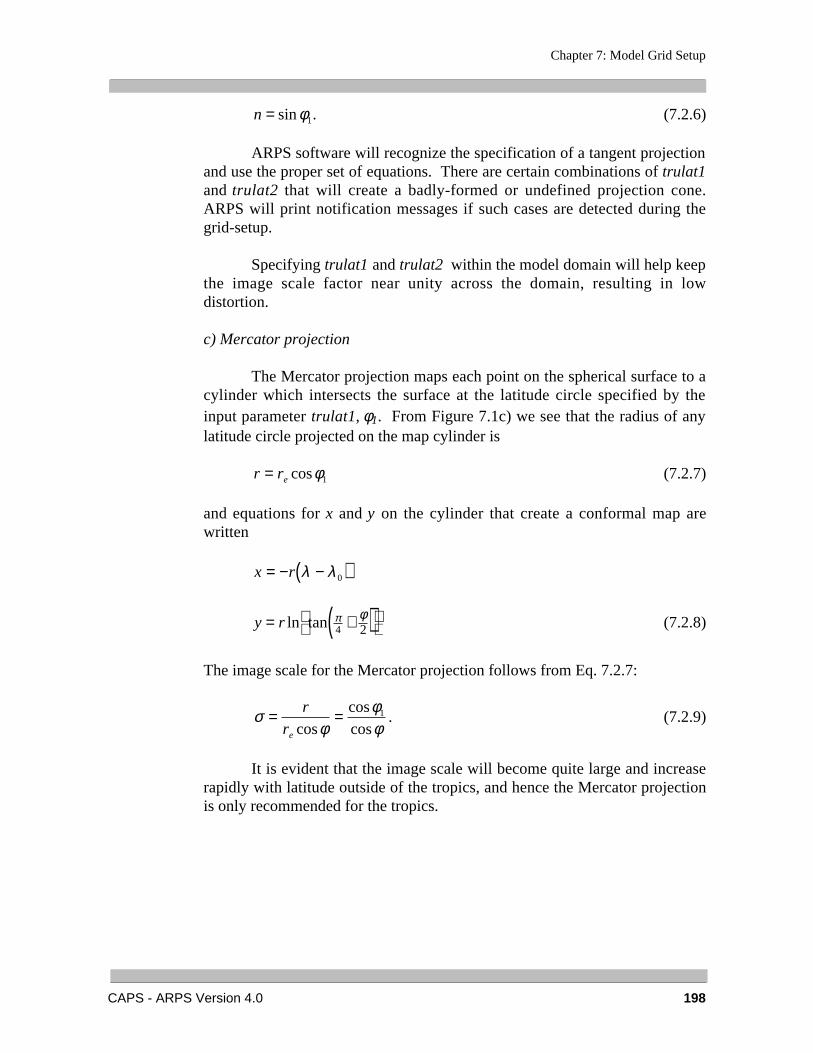
c) Mercator projection

The Mercator projection maps each point on the spherical surface to acylinder which intersects the surface at the latitude circle specified by theinput parameter trulat1, φ1. From Figure 7.1c) we see that the radius of anylatitude circle projected on the map cylinder is

r = re cosφ1 (7.2.7)

and equations for x and y on the cylinder that create a conformal map arewritten

x = −r λ − λ0( )

y r= +( )

ln tan π φ

4 2 (7.2.8)

The image scale for the Mercator projection follows from Eq. 7.2.7:

σ = r

re cosφ= cosφ1

cosφ. (7.2.9)

It is evident that the image scale will become quite large and increaserapidly with latitude outside of the tropics, and hence the Mercator projectionis only recommended for the tropics.



7.3. Vertical Coordinate Transformation _______________________

7.3.1. The computational coordinate transformation

A general curvilinear coordinate system is used by ARPS (seeAppendix B). The irregular grid associated with the curvilinear coordinate inthe physical space is mapped to a regular, rectangular computational gridthrough a coordinate transformation. All calculations are then carried out inthe computational space, using standard algorithms that are developed forCartesian systems. The regular shape of computational boundaries alsosimplifies implementation of boundary conditions.

In ARPS, the transformation Jacobians are calculated numerically onthe computational grid, so that the vertical transformed coordinate can begenerally defined.

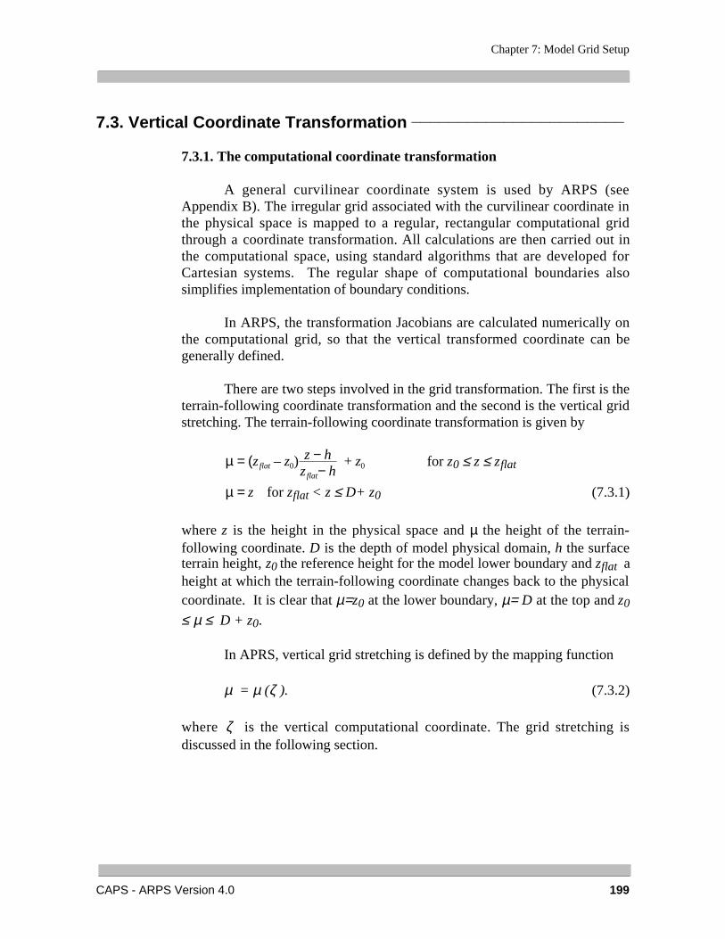
There are two steps involved in the grid transformation. The first is theterrain-following coordinate transformation and the second is the vertical gridstretching. The terrain-following coordinate transformation is given by

µ = (zflat – z0)z − h

zflat− h+ z0 for z0 ≤ z ≤ zflat

µ = z for zflat < z ≤ D+ z0 (7.3.1)

where z is the height in the physical space and µ the height of the terrain-following coordinate. D is the depth of model physical domain, h the surfaceterrain height, z0 the reference height for the model lower boundary and zflat aheight at which the terrain-following coordinate changes back to the physicalcoordinate. It is clear that µ=z0 at the lower boundary, µ= D at the top and z0

≤ µ ≤ D + z0.

In APRS, vertical grid stretching is defined by the mapping function

µ = µ (ζ ). (7.3.2)

where ζ is the vertical computational coordinate. The grid stretching isdiscussed in the following section.



7.3.2. Vertical grid stretching

Two grid stretching options are presently available in ARPS. One usesa cubic function and the other uses a hyperbolic tangent function. Both havethe prevision for defining layers of uniform grid near the ground and near thetop boundary. The details are given in next subsection.

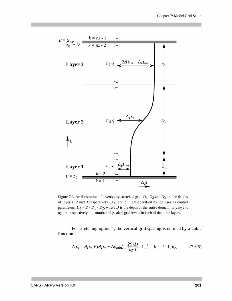
As illustrated in Fig. 7.3, the vertical extent of the model is dividedinto three layers. The lowest layer (layer 1) has a uniform resolution of ∆µl=

∆µmin. The middle layer (layer 2) has a grid spacing that increases from ∆µm

at its lowest level to ∆µu= 2∆µm - ∆µmin at its top, where ∆µm is the averagegrid spacing of this layer. Above, in layer 3, the spacing is constant and isapproximately equal to ∆µu (an adjustment to ∆µu may be required to insurethat the specified depth 3 contains an integral number of levels).

According to Figure 7.3,

n1 = D1/∆µmin, n2 = D2/∆µm and n3 = D3/∆µu,n1 + n2+ n3 = nz - 3, (7.3.3)D1 + D2 + D3 = D.

In Eq. (7.3.3), all parameters are known except for ∆µm. It is required

that ∆µm satisfy the following relation:

D1

∆µmin+

D2

∆µm+

D3

2∆µm – ∆µmin=

D∆ζ = nz – 3. (7.3.4)

where nz - 3 is the total number of grid levels between the bottom and topboundaries. ∆ζ is the grid spacing in the computation space, which is theaverage grid spacing in the entire domain.

Equation (7.3.4) is solved for ∆µm. The grid spacing in layers 1 and 3is then known. The spacing in layer 2 will be obtained from certain stretchingfunctions under the constraint that the average grid spacing is ∆µm and the

spacing at the bottom and top of this layer are respectively ∆µmin and 2∆µm -

∆µmin. These constraints can be satisfied by any odd function.



k = 1

k = 2

Layer 1

k

µ = z 0

∆ µminn1

Layer 2

Layer 3

n 2

n3

D2

D3

∆ µm

∆ µ

2∆ µm − ∆ µmin

k = nz - 2

k = nz - 1

D1

µ = µ top

0= z + D

Figure 7.3. An illustration of a vertically stretched grid. D1, D2 and D3 are the depths

of layer 1, 2 and 3 respectively. D1, and D2 are specified by the user as control

parameters. D3 = D - D1 - D2, where D is the depth of the entire domain. n1, n2 and

n3 are, respectively, the number of (scalar) grid levels in each of the three layers.

For stretching option 1, the vertical grid spacing is defined by a cubicfunction:

∆ µi = ∆µm + (∆µm − ∆µmin) [ 2(i-1) n2-1

- 1 ]3 for i =1, n2, (7.3.5)



for the mid-layer (layer 2), where i is the index for the vertical grid levels inthis layer and is directly related to the computational coordinate ζ. n2 is thenumber of levels.

For stretching option 2, the vertical grid spacing is defined by ahyperbolic tangent function:

∆ µi = ∆µm + ∆µmin – ∆µm

tanh 2α tanh2α

1 – ai – a for i =1, n2, (7.3.6)

where a = (1+n2)/2 and α is a tuning parameter which can take a valuebetween 0.2 and 5.0. The tuning parameter is set in the source code; ARPS 4.0is delivered with α = 1.0. For larger values of α , ∆µi tends to vary more

linearly with increasing i while for a smaller value of α, ∆µi changes more

abruptly at around i = n2/2 (see examples in Fig. 7.5). When ∆µi is known,

the height µ of the coordinate surface (defined as a w point) is obtained by

vertical summation of µi . When the vertical grid is uniform, ∆ µi = ∆ζ and µ= ζ.

Figures 7.4 and 7.5 show several examples of the vertical gridstretching.



0

200

400

600

800

1000

0 5 10 15 20 25 30 35

cnst.cubictanh

k

∆z

(m)

0

2000

4000

6000

8000

1 10 4

1.2 10 4

1.4 10 4

1.6 10 4

0 5 10 15 20 25 30 35

cnst.cubictanh

k

z (m

)

Figure 7.4. The vertical grid spacing ∆z (upper panel) and the physical height z

(lower panel) of the vertical grid levels as functions of the level index k, non-

stretching grid and for stretching options 1 and 2. For these cases, nz=35, D=16 km,

D1=0 m, D2=16 km and ∆zmin=50m. It can be seen that for stretching option 1, ∆z

increases rapidly near the top and bottom of the vertical domain, while option 2 hasthe fastest increase in ∆z at k~nz/2.



k

0

200

400

600

800

1000

0 5 10 15 20 25 30 35

∆z

(m)

= 0.2 = 1.0 = 5.0αα

α

0

2000

4000

6000

8000

1 104

1.2 104

1.4 104

1.6 104

0 5 10 15 20 25 30 35k

z (m

)

= 0.2 = 1.0 = 5.0αα

α

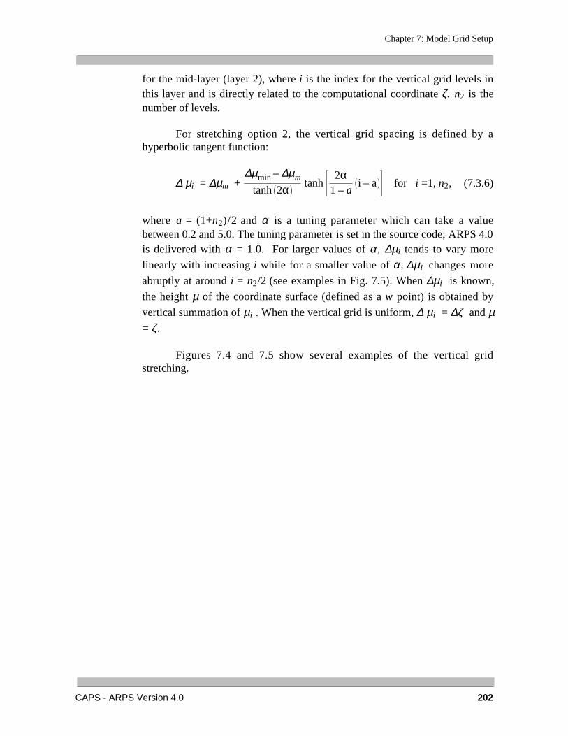
Figure 7.5. The vertical grid spacing ∆z (upper panel) and the physical height z

(lower panel) of the vertical grid levels as functions of the level index k, for the

tuning factor α = 0.2, 1.0, 5.0 for stretching option 2. In these cases, nz=35, D=16

km, D1=200 m, D2=9800 m and ∆zmin=50m. It can be seen that ∆z remains constant

in layer 1 and layer 3, and increases almost linearly with k for α=0.2 case but very

rapidly at the mid-levels for α=5.0.



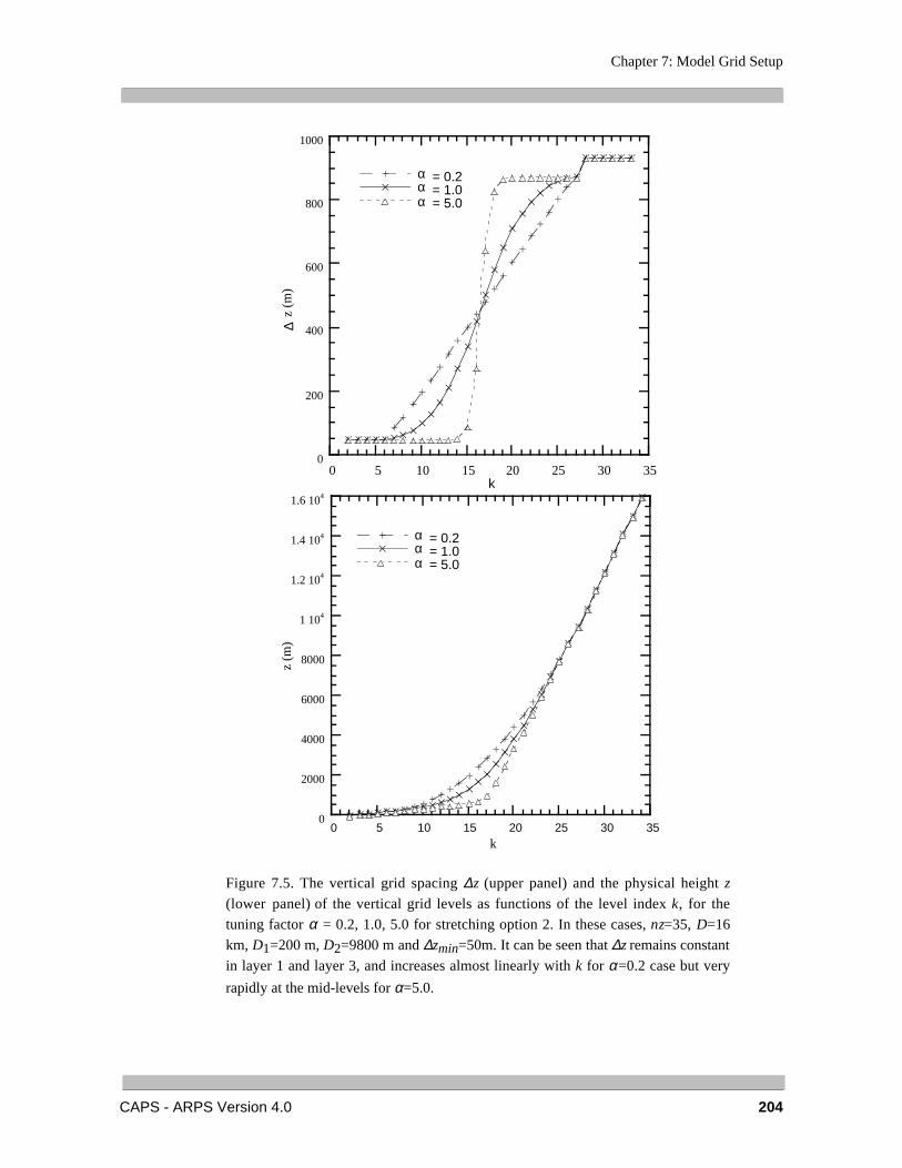
To conclude this section, we comment that the options for coordinatetransformations available in ARPS cover only a few possibilities. A user candefine his/her own coordinate transformation by editing the source code insubroutine INIGRD, where array zp (the vertical coordinate of w-points inphysical space) is initialized. When doing so it is recommended, though notrequired, that the zp(nz-1)-zp(2) be equal to (nz-3) dz in the absence of terrain,where dz is the constant computational grid spacing. The Jacobians are thencalculated from zp using finite differences. In Figure 7.6, an example ofARPS grid uses stretching option 2 and the transformation relation (7.3.1).

0

2

4

6

8

10

12

14

16

0 10 20 30 40 50

z (k

m)

x (km)

Z

Z

Z

top

flat

0

Figure 7.6. An illustration of ARPS computational domain using coordinate transformationrelation (7.3.1) and grid stretching option 2 (Eq. (7.3.6)). zflat =10 km, nz=35, D=16 km,

D1=200 m, D2=9800 m, ∆zmin=50 m and α=1.0. Only every other grid line is plotted in the

vertical direction.



7.4. Adaptive Grid Refinement and Two-way Interactive GridNesting _________________________________________

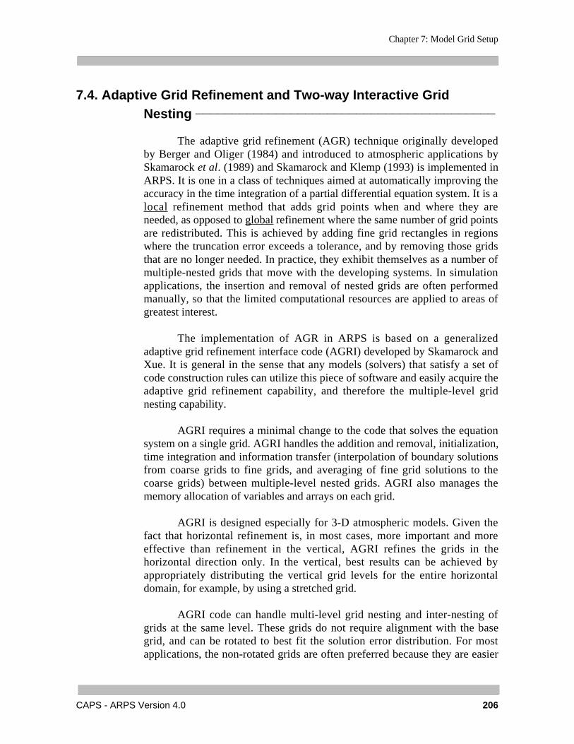
The adaptive grid refinement (AGR) technique originally developedby Berger and Oliger (1984) and introduced to atmospheric applications bySkamarock et al. (1989) and Skamarock and Klemp (1993) is implemented inARPS. It is one in a class of techniques aimed at automatically improving theaccuracy in the time integration of a partial differential equation system. It is alocal refinement method that adds grid points when and where they areneeded, as opposed to global refinement where the same number of grid pointsare redistributed. This is achieved by adding fine grid rectangles in regionswhere the truncation error exceeds a tolerance, and by removing those gridsthat are no longer needed. In practice, they exhibit themselves as a number ofmultiple-nested grids that move with the developing systems. In simulationapplications, the insertion and removal of nested grids are often performedmanually, so that the limited computational resources are applied to areas ofgreatest interest.

The implementation of AGR in ARPS is based on a generalizedadaptive grid refinement interface code (AGRI) developed by Skamarock andXue. It is general in the sense that any models (solvers) that satisfy a set ofcode construction rules can utilize this piece of software and easily acquire theadaptive grid refinement capability, and therefore the multiple-level gridnesting capability.

AGRI requires a minimal change to the code that solves the equationsystem on a single grid. AGRI handles the addition and removal, initialization,time integration and information transfer (interpolation of boundary solutionsfrom coarse grids to fine grids, and averaging of fine grid solutions to thecoarse grids) between multiple-level nested grids. AGRI also manages thememory allocation of variables and arrays on each grid.

AGRI is designed especially for 3-D atmospheric models. Given thefact that horizontal refinement is, in most cases, more important and moreeffective than refinement in the vertical, AGRI refines the grids in thehorizontal direction only. In the vertical, best results can be achieved byappropriately distributing the vertical grid levels for the entire horizontaldomain, for example, by using a stretched grid.

AGRI code can handle multi-level grid nesting and inter-nesting ofgrids at the same level. These grids do not require alignment with the basegrid, and can be rotated to best fit the solution error distribution. For mostapplications, the non-rotated grids are often preferred because they are easier



to handle for post-processing purposes. The aligned grids also facilitate theuse of conservative interpolation schemes between coarse and fine gridsolutions. In theory, AGRI allows for any level of grid nesting. In practice, 2to 4 levels of nesting are most commonly used. An example of the applicationof AGRI in ARPS can be found in Xue et al., (1993). In that paper, asimulation of small tornado vortices within a supercell storm is presentedwhich used four levels of grid nesting. The finest grids have a horizontalresolution of about 55 m, while the base grid resolution is 1 km.

The source code for AGRI is usually contained in a separate directoryfrom that of ARPS. The compilation and linking of ARPS subroutines arehandled automatically by makefiles. The AGRI code is written forconventional vector computers, and does not work well on MPP machines.The AGRI source code is not currently distributed with the current officialrelease of ARPS. Users who are interested in this capability should [email protected] or [email protected].

7.5. One Way Interactive Self-Nesting _________________________

One way interactive self-nesting between successive runs of differentresolutions can be easily performed with ARPS using the utility program,ARPSR2H (see Section 10.5). ARPSR2H interpolates the output from a largerdomain run in either restart file or history dump format onto a smaller sub-domain of specified resolution, then writes out data files that can be used toinitialize the smaller domain and provide the boundary forcing. ARPSstandard input file, arps40.input, is used by ARPSR2H, arps40.input has anextra namelist block called &gridinit that is used only by ARPSR2H to definethe smaller grid. When the external boundary condition data dump flagexbcdmp is turned on, ARPSR2H writes out external boundary forcing filesfor the fine grid at the same time history data are written out. The fine grid caneither be initialized using interpolated coarse fields (from history format datacreated by ARPSR2H) or using analysis fields.

The command to compile and link ARPSR2H is

makearps arpsr2h

and the command to execute is

ext2arps < arps40.input.



For further information on initializing ARPS with a 3-D data set andon forcing ARPS using external data sets, the reader is referred to Chapter 8.

7.6. Grid Translation Features _______________________________

Because of computer memory limitations, numerical modelers mustdecide for each experiment how their computational domain extent should besacrificed in favor of grid resolution (and vice versa). Ideally, one would likea grid spacing fine enough to resolve the phenomena of interest and a domainsize large enough that the placement of the boundaries would not undulycontaminate the solution, at least for the time scales of interest. One approachis to make use of nested or adaptive grids (see previous section). Anotherapproach, described in this section, is to use a moving reference frame to keepthe features of interest within the computational grid.

7.6.1. User-specified grid motion

When creating thunderstorm simulations, the user can reduce the totalnumber of grid points needed by specifying a storm-following grid. Themotion of the grid can be explicitly controlled by setting grdtrns = 1 in theinput file and specifying input parameters umove and vmove which representthe components of grid motion during the simulation. However, since it isoften not possible to know in advance what the storm motion will be, it maybe preferable to apply one of the automatic grid-translation proceduresdescribed in the next few sub-sections (namely, cell tracking or optimalpattern translation techniques).

7.6.2. Cell tracking algorithm

ARPS includes a cell-tracking algorithm based, in part, on the radarcell tracking technique of Witt and Johnson (1993). This algorithm identifiesconvective cells and tracks their locations during a simulation. The location,size, direction and speed of motion of each cell are stored in a file for analysisand display. The cell tracking algorithm can be used as a "stand-alone"procedure or as the basis for a moving reference frame. The cell trackingalgorithm is turned on by setting cltkopt = 1. To define a moving referenceframe in terms of the motion of the vertical velocity centroid of theseconvective cells, i.e., to use the above algorithm to define the domaintranslation, one should specify grdtrns = 2 in the input file. In this case,cltkopt is reset to 1 if not already so.



If grdtrns = 2, the simulation begins with a umove and vmove based onthe mean wind in the lowest 5 km. As vertical velocity develops, the center ofmass of updrafts exceeding 5 ms-1 is computed. The center of masscalculation uses data only at grid points below 12 km. After a sequence ofupdraft centroids has been identified, a least-squares technique finds the recentmovement of the centroid and umove and vmove are modified to correct forthe actual storm motion or development.

The cell tracking process produces a file named runname.track. Thisfile contains a record of the cells identified during each call to the cell trackingsubroutine, CELTRK. The cell absolute positions, their volumes (measured asnumber of grid cells having vertical velocity greater than 5 ms-1) and motionare recorded. Software is available to plot these tracks as a function of time inabsolute coordinates.

It is important to note that a number of adjustable parameters are usedin the cell-tracking algorithm. These parameters include the maximumnumber of cells to be tracked, the threshold vertical velocity defining a “cell,”the minimum horizontal area of a cell, etc. Please examine subroutineCELTRK for more details.

7.6.3. Optimal pattern translation

The translational motion of a scalar pattern determined objectivelyfrom real or model data can also used to define a moving reference frame.The technique described herein is based on a least squares technique proposedby Gal-Chen (1982). We consider the frozen-turbulence approximation(Taylor’s hypothesis) as applied to the motion of a scalar quantity φ,

∂φ∂t

+ U∂φ∂x

+ V∂φ∂y

= 0 , (7.6.1)

where U and V are constants. It can be verified that the solution of (7.6.1) is

φ = f(x - Ut, y - Vt),

where f is any arbitrary function of two variables. Introducing the Galileantransformation x' = x - Ut and y' = y - Vt, the solution can be written as φ =f(x', y'), in which there is no time dependence. The Galilean transformationhas a simple physical interpretation: the new coordinate system is moving atthe speed U in the x-direction and speed V in the y-direction with respect tothe original coordinate system. Thus, a pattern satisfying (7.6.1) would appear



stationary in a frame of reference moving with velocity components U and V.Alternatively, we can say that (7.6.1) describes the translation of a scalarpattern at speeds U and V in a fixed reference frame.

Although there is no a priori reason why a scalar (e.g., vertical veloc-ity or rainwater) should satisfy the frozen-turbulence approximation (7.6.1),experience has shown that meteorological phenomena over a wide range ofscales often appear as organized structures or patterns that “advect” or“propagate” at some characteristic speed, at least for certain periods of time.The U and V components describing this pattern-translation are notnecessarily associated with the mean fluid velocity, although there often is aclose correspondence between the two. Further discussions of thisapproximation and its limitations can be found in Hinze (1975), Townsend(1976), Panofsky and Dutton (1984) and in references therein.

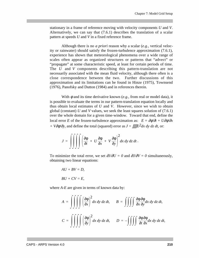
With φ and its time derivative known (e.g., from real or model data), itis possible to evaluate the terms in our pattern-translation equation locally andthus obtain local estimates of U and V. However, since we wish to obtainglobal (constant) U and V values, we seek the least squares solution of (7.6.1)over the whole domain for a given time-window. Toward that end, define thelocal error E of the frozen-turbulence approximation as: E = ∂φ/∂t + U∂φ/∂x

+ V∂φ/∂y, and define the total (squared) error as J = ∫∫∫∫E2dx dy dz dt, or:

J =

∂φ∂t

+ U∂φ∂x

+ V∂φ∂y

2

dx dy dz dt .

To minimize the total error, we set ∂J/∂U = 0 and ∂J/∂V = 0 simultaneously,obtaining two linear equations:

AU + BV = D,

BU + CV = E,

where A-E are given in terms of known data by:

A =

∂φ∂x

2dx dy dz dt, B =

∂φ∂x

∂φ∂y

dx dy dz dt,

C =

∂φ∂y

2dx dy dz dt, D = –

∂φ∂t

∂φ∂x

dx dy dz dt,



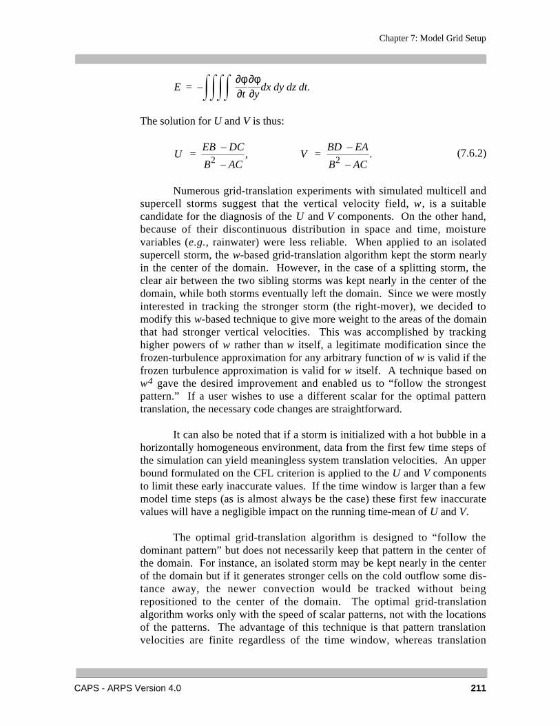
E = –

∂φ∂t

∂φ∂y

dx dy dz dt.

The solution for U and V is thus:

U =

EB – DC

B2 – AC, V =

BD – EA

B2 – AC. (7.6.2)

Numerous grid-translation experiments with simulated multicell andsupercell storms suggest that the vertical velocity field, w , is a suitablecandidate for the diagnosis of the U and V components. On the other hand,because of their discontinuous distribution in space and time, moisturevariables (e.g., rainwater) were less reliable. When applied to an isolatedsupercell storm, the w-based grid-translation algorithm kept the storm nearlyin the center of the domain. However, in the case of a splitting storm, theclear air between the two sibling storms was kept nearly in the center of thedomain, while both storms eventually left the domain. Since we were mostlyinterested in tracking the stronger storm (the right-mover), we decided tomodify this w-based technique to give more weight to the areas of the domainthat had stronger vertical velocities. This was accomplished by trackinghigher powers of w rather than w itself, a legitimate modification since thefrozen-turbulence approximation for any arbitrary function of w is valid if thefrozen turbulence approximation is valid for w itself. A technique based onw4 gave the desired improvement and enabled us to “follow the strongestpattern.” If a user wishes to use a different scalar for the optimal patterntranslation, the necessary code changes are straightforward.

It can also be noted that if a storm is initialized with a hot bubble in ahorizontally homogeneous environment, data from the first few time steps ofthe simulation can yield meaningless system translation velocities. An upperbound formulated on the CFL criterion is applied to the U and V componentsto limit these early inaccurate values. If the time window is larger than a fewmodel time steps (as is almost always be the case) these first few inaccuratevalues will have a negligible impact on the running time-mean of U and V.

The optimal grid-translation algorithm is designed to “follow thedominant pattern” but does not necessarily keep that pattern in the center ofthe domain. For instance, an isolated storm may be kept nearly in the centerof the domain but if it generates stronger cells on the cold outflow some dis-tance away, the newer convection would be tracked without beingrepositioned to the center of the domain. The optimal grid-translationalgorithm works only with the speed of scalar patterns, not with the locationsof the patterns. The advantage of this technique is that pattern translationvelocities are finite regardless of the time window, whereas translation



velocities based on the locations of patterns can become quite large(theoretically infinite in the case of discontinuous propagation, i.e., new cellformation) and can be quite sensitive to the duration of the time window.

The optimal grid translation subroutines can be found in filegrdtrns3d.f. Subroutine ADJUVMV (which calls GALILEI) adjusts themodel variables at the past and present model time levels (see next section)whenever the domain translation speed changes, regardless of the algorithmthat caused the change in the domain translation speed (user-specified change,automatic grid translation, cell-tracking update, etc.). SubroutineAUTOTRANS computes the optimum (least squares) pattern translationspeed.

7.6.4. Redefining quantities in a moving reference frame

Once the grid translation velocity is determined (e.g., by the celltracking procedure or optimal pattern translation procedure), all modelvariables are redefined in the moving reference frame. This redefinition alsooccurs if the model is initialized from a restart file in which the umove andvmove components differ from those in the current input file. The appropriateredefinition for the current values of the horizontal wind field u, and v, and forall scalars φ is:

u = u - Uv = v - Vφ = φ

where U and V are the new system translation components (or the change inthe system translation components if the old system was already translated).Because ARPS currently uses the leapfrog scheme to integrate the governingequations, model variables at both present and past time levels must beredefined in the moving reference frame. However, care must be taken thatthe time derivative of the transformed variables (based on present and pastvalues) satisfies the Galilean transformation: ∂/∂t = ∂/∂t' - U ∂/∂x' - V ∂/∂y'.The necessity for this condition can be seen by considering the example of aflow that is stationary in a moving reference frame. Such a flow would not bestationary in a fixed reference frame (it would appear as a translating pattern),hence the local derivatives in the fixed and moving reference frames shouldnot be the same.

An appropriate redefinition for the 2 time levels is,

At the "present" time:



u(i,j,k,tpresent) = u(i,j,k,tpresent) - Uv(i,j,k,tpresent) = v(i,j,k,tpresent) - Vφ(i,j,k,tpresent) = φ(i,j,k,tpresent)

At the "past" time:

u(i,j,k,tpast) = u(i,j,k,tpast) - U - U ∆t ∂u/∂x - V ∆t ∂u/∂y

v(i,j,k,tpast) = v(i,j,k,tpast) - V - U ∆t ∂v/∂x - V ∆t ∂v/∂y

φ(i,j,k,tpast) = φ(i,j,k,tpast) - U ∆t ∂φ/∂x - V ∆t ∂φ/∂y

where ∆t is the model big time step.Currently, centered space derivatives are used to approximate the

spatial derivatives. The time level of the spatial derivatives is half-waybetween the past and present time levels (i.e., an average is taken).

7.6.5. Some practical considerations

In the current version of the code, the user is asked to specify severalgrid translation input parameters in ARPS input file. The parameter grdtrnsdetermines which algorithm is used to compute the system translationcomponents. If grdtrns = 1 then U and V are just the user-specified valuesumove and vmove. If grdtrns = 2 then U and V are determined from the cell-tracking algorithm (see Section 7.5.2). If grdtrns = 3 then U and V aredetermined from the optimal pattern translation technique described in Section7.5.3.

If grdtrns = 3 (optimal pattern translation) the user must also specifytwo additional parameters: chkdpth and twindow. The chkdpth parameter setsthe depth above the k=3 physical grid point over which U and V are calculated(the reason the minimum k level is set to 3 is because the optimal patterntranslation is based on the vertical velocity field, which first becomes non-zero at level 3). The user is cautioned that chkdpth should be ≥ dz. Thetwindow parameter sets the time interval (in seconds) between successiveupdates of the grid translation speed. twindow also defines the interval overwhich the running average of the system translation speed is computed.

Chapter 7: Model Grid Setup 7 Map Projection, Model … Map Projection, Model Grid Setup and Grid...

Documents

Transcript of Chapter 7: Model Grid Setup 7 Map Projection, Model … Map Projection, Model Grid Setup and Grid...