Chapter 7 Flow of a Real Fluid - Seoul National University

Ch. 7 Flow of a Real Fluid

7-1

Chapter 7 Flow of a Real Fluid

7.1 Laminar Flow

7.2 Turbulent Flow and Eddy Viscosity

7.3 Fluid Flow Past Solid Boundaries

7.4 Characteristics of Boundary Layers

7.5 The Laminar Boundary Layer*

7.6 The Turbulent Boundary Layer*

7.7 Separation

7.8 Secondary Flow

7.9 Flow Establishment

7.10 Shear Stress and Head Loss

7.11 Shear Stress Effects

7.12 Velocity Distribution

7.13 Separation – Internal Flow

7.14 Secondary Flow– Internal Flow


7-2

7.15 Navier-Stokes Equation for Two-Dimensional Flow*

7.16 Applications of the Navier-Stokes Equations*

Objectives:

- Introduce the concepts of laminar and turbulent flow

- Examine the condition under which laminar and turbulent flow occur

- Introduce influence of solid boundaries on qualitative views

- Derive Navier-Stokes equation for two-dimensional flow and discuss its applications


7-3

7.0 Introduction

• Ideal fluid

- In Chs.1 ~ 5, the flow of an ideal incompressible fluid was considered.

- Ideal fluid was defined to be inviscid, devoid of viscosity.

- There were no frictional effects between moving fluid layers or between the fluid and

bounding walls.

• Real Fluid

- Viscosity introduces resistance to motion by causing shear or friction forces between

fluid particles and between these and boundary walls.

- For flow to take place, work must be done against these resistance forces. In this

process energy is converted into heat (mechanical energy loss).

Ideal (inviscid) fluid Real (viscous) fluid

Viscosity inviscid viscous

Velocity profile Uniform (slip condition) non-uniform(no-slip)

Eq. of motion Euler's equation Navier-Stokes equation

(Nonlinear, 2nd-order P.D.E)


7-4

7.1 Laminar flow

• Laminar flow

- Agitation of fluid particles is a molecular nature only.

- Length scale ~ order of mean free path of the molecules

- Particles appear to be constrained to motion in parallel paths by the action of viscosity.

- Viscous action damps disturbances by wall roughness and other obstacles.

→ stable flow

- The shearing stress between adjacent layers is

dv

dy (1.12)

Fig. 7.1

• Turbulent flow

- Fluid particles do not retain in layers, but move in heterogeneous fashion through the flow.

- Particles are sliding past other particles and colliding with some in an entirely random

manner.

- Rapid and continuous macroscopic mixing of the flowing fluid occurs.

- Length scale of motion >> molecular scales in laminar flow


7-5

• Two forces affecting motion

(i) Inertia forces, IF

~ acceleration of motion

23 2 2

I

VF M a l V l

l

(ii) Viscous forces, VF

22

V

dV V lF A l V l

dy l

• Reynolds number eR

2 2I

eV

F V l Vl Vl VlR

F Vl

-1 -1dynamic viscosity (kg m s )

2kinematic viscosity (m s)


7-6

• Inertia forces are dominant → turbulent flow

Viscous forces are dominant → laminar flow

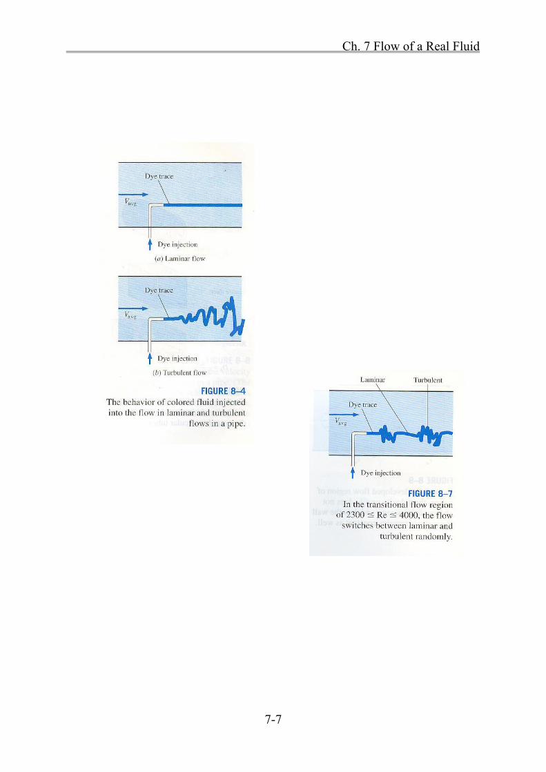
• Reynolds dye stream experiments

low velocity → low Reynolds number → laminar flow

high velocity → high Reynolds number → turbulent flow

• Critical velocity

upper critical velocity: laminar → turbulent

lower critical velocity: turbulent → laminar

• Critical Reynolds number

(i) For pipe flow

, pipe diametere

VdR d

(7.1)

12100 laminar flow lower critical 2100e cR R

22100 4000 transition upper critical 4000e cR R

4000 turbulent floweR


7-7


7-8


7-9

(ii) Open channel flow: 500 laminar floweR

(4 )2100 500c c

Vd V R VRR R

2 4hydraulic radius

4

d dR A

d

(iii) Flow about a sphere: 1 laminar floweR

where V = approach velocity; d = sphere diameter

• Experiment for two flow regimes

i) As V is increased → OABCD

OB (laminar flow) → BC (transition region) → CD (turbulent flow)

ii) As V is decreased → DCAO

DC (turbulent) → CA (transition) → AO (laminar flow)

upper critical velocity

lower critical velocity


7-10

[IP 7.1] Water at 15˚C flows in a cylindrical pipe of 30 mm diameter.

6 21.339 10 m s water at 15 C p.694 A. 2.4b

Find largest flow rate for which laminar flow can be expected.

[Sol]

Take 2100c

R as the conservative upper limit for laminar flow

(a) For water

3

6

30 102100

1.139 10c

VVdR

0.080 m swaterV

2 5 30.0805 0.03 5.69 10 m s4waterQ

(4.4)

(b) For air

5 21.46 10 m sair 5 31.8 10 pa s 1.225 kg mair

1.022 m sairV (7.1)

4 37.22 10 m s 13air waterQ Q (4.4)

air water

, ,c air c waterV V


7-11

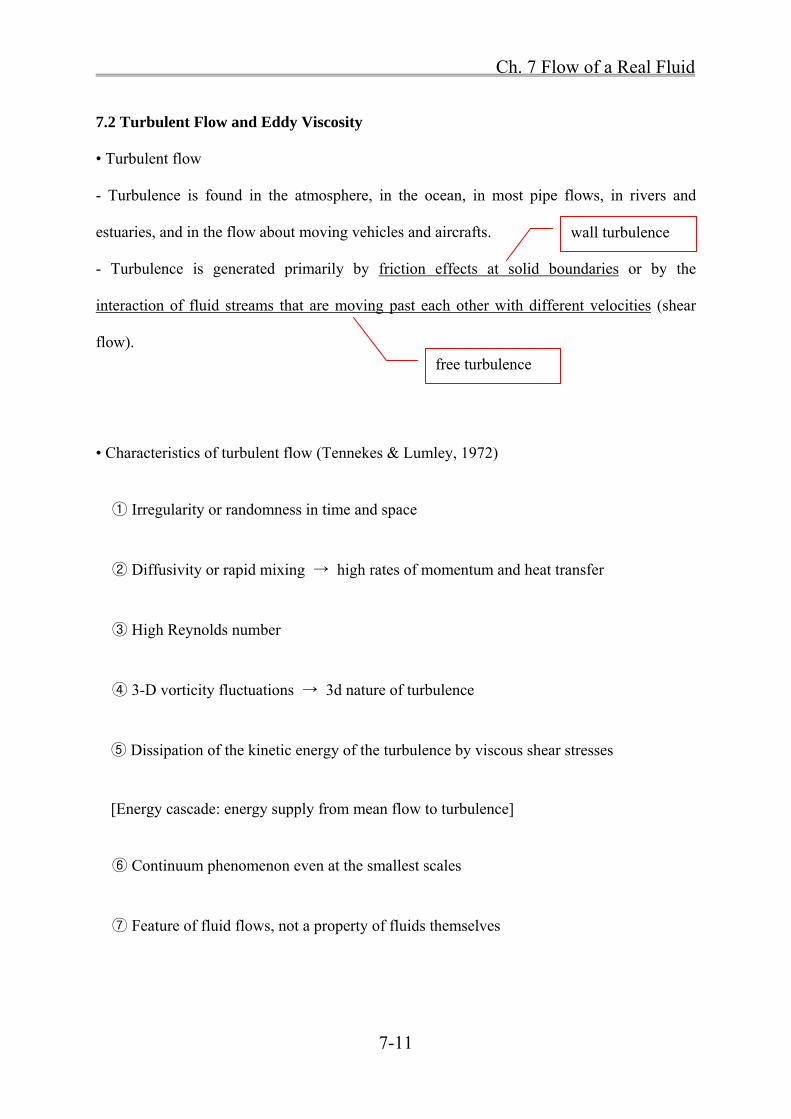
7.2 Turbulent Flow and Eddy Viscosity

• Turbulent flow

- Turbulence is found in the atmosphere, in the ocean, in most pipe flows, in rivers and

estuaries, and in the flow about moving vehicles and aircrafts.

- Turbulence is generated primarily by friction effects at solid boundaries or by the

interaction of fluid streams that are moving past each other with different velocities (shear

flow).

• Characteristics of turbulent flow (Tennekes & Lumley, 1972)

① Irregularity or randomness in time and space

② Diffusivity or rapid mixing → high rates of momentum and heat transfer

③ High Reynolds number

④ 3-D vorticity fluctuations → 3d nature of turbulence

⑤ Dissipation of the kinetic energy of the turbulence by viscous shear stresses

[Energy cascade: energy supply from mean flow to turbulence]

⑥ Continuum phenomenon even at the smallest scales

⑦ Feature of fluid flows, not a property of fluids themselves

wall turbulence

free turbulence


7-12

• Decomposition of turbulent flow

'x xv t v v

'y yv t v v

'v t instantaneous turbulent velocity

v time mean velocity '

0

1 Tv t dt

T

xv turbulent fluctuation in x-direction

yv turbulent fluctuation in y-direction

0

10

T

x xv v dtT

0yv

Fig. 7.4


7-13

• 1 2

2 2

0

1rms

T

x xv v dtT

• Relative intensity of turbulence 2

xv

v

• Mean time interval, T

T = times scale = meaningful time for turbulence fluctuations

- air flow: 1 010 ~ 10 sec

- pipe flow: 1 010 ~ 10 sec

- open flow: 0 110 ~ 10 sec

~ measure of the scale of the turbulence

~ size of the turbulent eddies size of boundary

~ order of (pipe radius, channel width or depth, boundary layer thickness)

→ The intensity of turbulence increases with velocity, and scale of turbulence increases with

boundary dimensions.


7-14

[Re] Measurement of turbulence

(i) Hot-wire anemometer

~ use laws of convective heat transfer

~ Flow past the (hot) sensor cools it and decrease its resistance and output voltage.

~ record of random nature of turbulence

(ii) Laser Doppler Velocitymeter (LDV)

~ use Doppler effect

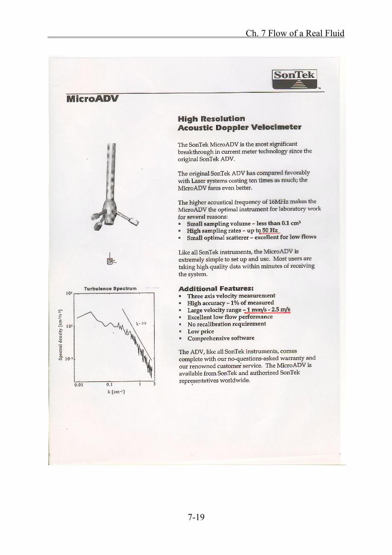
(iii) Acoustic Doppler Velocitymeter (ADV)

(iv) Particle Image Velocimetry (PIV)


7-15

Hot wire anemometer


7-16

Laser Doppler velocimetry


7-17


7-18

Acoustic Doppler Velocimeter


7-19


7-20

Particle Image Velocimetry


7-21

• Turbulence

- Because turbulence is an entirely chaotic motion of small fluid masses, motion of individual

fluid particle is impossible to trace.

→ Mathematical relationships may be obtained by considering the average motion of

aggregations of fluid particles or by statistical methods.

• Shearing stresses in turbulent flow

Let time mean velocity v v

Thus, velocity gradient is dv

dy

Now consider momentum exchange by fluid particles moved by turbulent fluctuation

Mass moved to the lower layer tends to speed up the slower layer v

Mass moved to the upper layer tends to slow down the faster layer v v

→ This is the same process as if there were a shearing stress between two layers.


7-22

• Problem of useful and accurate expressions for turbulent shear stress in terms of mean

velocity gradients and other flow properties

1) Boussinesq (1877)

~ suggest the similar equation to laminar flow equation

dv

dy (7.2)

= eddy viscosity

= property of flow (not of the fluid alone)

f (structure of the turbulence, space)

total

dv

dy

where = viscosity action, = turbulence action

2) Reynolds (1895)

~ suggest the turbulent shear stress with time mean value of the product of x yv v

x yv v ~ Reynolds stress

xv = fluctuating velocity along the direction of general mean motion

yv = fluctuating velocity normal to the direction of general mean motion

x yv v = time mean value of the product of 1

x y x yv v v v dtT


7-23

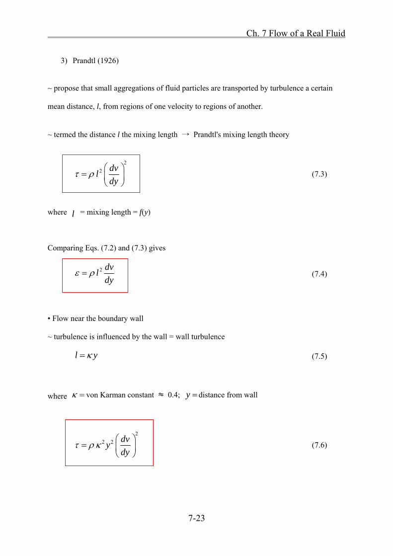
3) Prandtl (1926)

~ propose that small aggregations of fluid particles are transported by turbulence a certain

mean distance, l, from regions of one velocity to regions of another.

~ termed the distance l the mixing length → Prandtl's mixing length theory

2

2 dvl

dy

(7.3)

where l = mixing length = f(y)

Comparing Eqs. (7.2) and (7.3) gives

2 dv

ldy

(7.4)

• Flow near the boundary wall

~ turbulence is influenced by the wall = wall turbulence

l y (7.5)

where von Karman constant ≈ 0.4; y distance from wall

2

2 2 dvy

dy

(7.6)


7-24

[IP 7.2] Show that if laminar flow is parabolic velocity profile, the shear stress profile must

be a straight line.

[Sol]

dv

dy (1.12)

2

1 2 parabolicv C y C

12

dvC y

dy

1 straight line2 C y C y


7-25

[IP 7.3] A turbulent flow of water occurs in a pipe of 2 m diameter.

logarithmic10 0.8lnv y

1 3103 Pa

y m

Calculate , ,l

[Sol]

dv

dy (a)

2

2 dvl

dy

(b)

2

2 2 dvy

dy

(c)

1

1 3 1 3

0.82.4

y m y m

dvs

dy y

(a): 103 2.4 42.9 Pa s

(b): 23 2103 10 2.4l 0.134 m 10% of pipe radiusl

(c): 2

23 2 1103 10 2.4

3

0.401


7-26

7.3 Fluid Flow Past Solid Boundaries

• Flow phenomena near a solid boundary

- external flows: flow around an object immersed in the fluid

(over a wing or a flat plate, etc.)

- internal flows: flow between solid boundaries

(flow in pipes and channels)

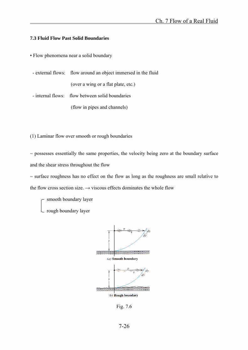
(1) Laminar flow over smooth or rough boundaries

~ possesses essentially the same properties, the velocity being zero at the boundary surface

and the shear stress throughout the flow

~ surface roughness has no effect on the flow as long as the roughness are small relative to

the flow cross section size. → viscous effects dominates the whole flow

smooth boundary layer

rough boundary layer

Fig. 7.6


7-27

(2) Turbulent flow over smooth or rough boundaries

- Flow over a smooth boundary is always separated from the boundary by a sublayer of

viscosity-dominated flow (laminar flow).

[Re] Existence of laminar sublayer

Boundary will reduce the available mixing length for turbulence motion.

→ In a region very close to the boundary, the available mixing length is reduced to zero (i.e.,

the turbulence is completely extinguished).

→ A film of viscous flow over the boundary results.

- Shear stress:

Inside the viscous sublayer: dv

dy

Outside the viscous sublayer:

2

2 dvl

dy

- Between the turbulent region and the viscous sublayer lies a transition zone in which shear

stress results from a complex combination of both turbulent and viscous action.

→ The thickness of the viscous sublayer varies with time. The sublayer flow is unsteady.

laminar flow

turbulent flow

transition flow


7-28

- Roughness of the boundary surface affects the physical properties (velocity, shear, friction)

of the fluid motion.

→ The effect of the roughness is dependent on the relative size of roughness and viscous

sublayer.

- Classification of surfaces based on ratio of absolute roughness e to viscous sublayer

thickness v

i) Smooth surface: 0.3v

e

- Roughness projections are completely submerged in viscous sublayer.

→ They have no effect on the turbulence.

ii) Transition: 0.3 10v

e

iii) Rough surface: 10v

e

- However, the thickness of the viscous sublayer depends on certain properties of the flow.

→ The same boundary surface behave as a smooth one or a rough one depending on the size

of the Reynolds number and of the viscous sublayer.

1v

ef R

) roughsurfacee vi v R

) smoothsurfacee vii v R


7-29

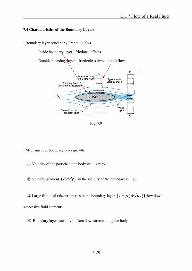
7.4 Characteristics of the Boundary Layers

• Boundary layer concept by Prandtl (1904)

- Inside boundary layer - frictional effects

- Outside boundary layer – frictionless (irrotational) flow

Fig. 7.9

• Mechanism of boundary layer growth

① Velocity of the particle at the body wall is zero.

② Velocity gradient dv dy in the vicinity of the boundary is high.

③ Large frictional (shear) stresses in the boundary layer dv dy slow down

successive fluid elements.

④ Boundary layers steadily thicken downstream along the body.


7-30

• Flow over a smooth flat plate

→ Boundary layer flow: laminar → transition → turbulent

Fig. 7.8

- Laminar boundary layer

~ Viscous action is dominant.

0x

V xR

500,000

cxR (7.7a)

0VR

4,000c

R (7.7b)

500,000xR or

4,000R → laminar boundary layer expected

- Turbulent boundary layer

~ Laminar sublayer exists.

500,000xR or

4,000R

turbulent flow

frictionless flow

transition flow

laminar flow


7-31

• Differences between Figs. 7.8 and 7.9

i) For the streamlined body, its surface has a curvature that may affect the boundary layer

development either due to inertial effect or induced separation if the body is particularly blunt.

(ii) For the streamlined body, the velocity in the irrotational flow (no vorticity)

0 ; 2d v u

dxdy x y

just outside the boundary layer, changes continuously along the body because of the

disturbance to the overall flow offered by the body of finite width.


7-32

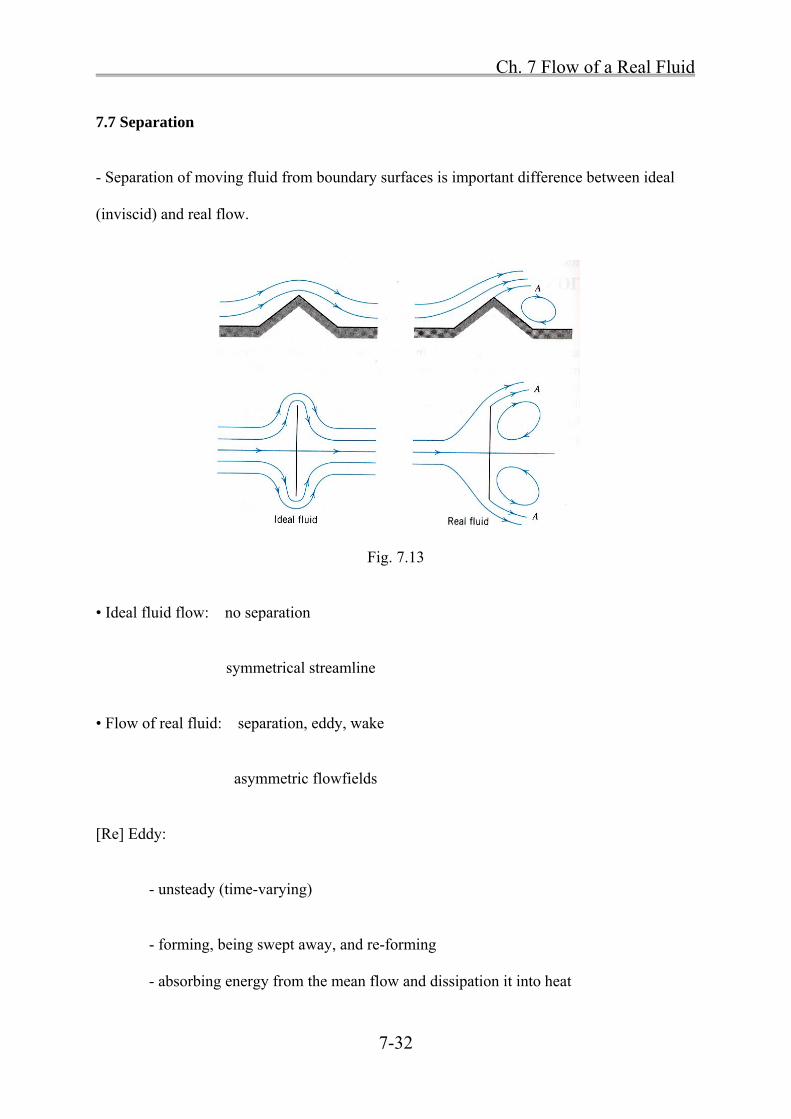
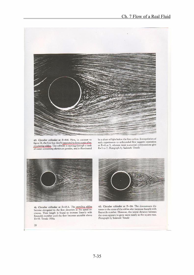
7.7 Separation

- Separation of moving fluid from boundary surfaces is important difference between ideal

(inviscid) and real flow.

Fig. 7.13

• Ideal fluid flow: no separation

symmetrical streamline

• Flow of real fluid: separation, eddy, wake

asymmetric flowfields

[Re] Eddy:

- unsteady (time-varying)

- forming, being swept away, and re-forming

- absorbing energy from the mean flow and dissipation it into heat


7-33

• Surface of discontinuity divide the live stream from the adjacent and more moving eddies.

→ Across such surfaces there will be a high velocity gradient and high shear stress.

→ no discontinuity of pressure

→ tend to break up into smaller eddies (Fig. 7.14b)

Fig. 7.14


7-34


7-35


7-36


7-37

• Free streamline:

Under special circumstances the streamlines of a surface of discontinuity become free

streamline.

Along the free streamline, the pressure is constant.

Fig. 7.15

• Separation point

The prediction of separation may be simple for sharp-cornered obstructions.

However, prediction is more complex matter for gently curved (streamlined) objects or

surfaces.

→ The analytical prediction of separation point location is an exceedingly difficult problem.

→ Thus, it is usually obtained more reliably from experiments.

• For small ratio of thickness to length → no separation (Fig. 7.13)

For large ratio of thickness to length → separation (Fig. 7.14)


7-38

Fig. 7.17

Proceeding from A to B, the pressure falls because the flow is accelerating.

→ This produces a favorable pressure gradient which strengthens the boundary layer.

From B to C, the pressure rises as the flow decelerates because the body is thinning.

→ This produces a adverse (unfavorable) pressure gradient which weakens the boundary

layer sufficiently to cause separation.

• Acceleration of real fluids tends to be an efficient process, deceleration an inefficient one.

Accelerated motion: stabilize the boundary layer, minimize energy dissipation

Decelerated motion: promote separation, instability, eddy formation, and large energy

dissipation


7-39

7.8 Secondary Flow

Another consequence of wall friction is the creation of a flow within a flow, a secondary flow

superposed on the main primary flow.

Fig. 7.18

1) Secondary flow occurring at the cross section of the meandering river: Fig. 7.18a)

2) Horseshoe-shaped vortex around the bridge pier: Fig. 7.18b)

~ Downward secondary flow from A to B induces a vortex type of motion, the core of the

vortex being swept downstream around the sides of the pier.

~ This principle is used on the wings of some jet aircraft, vortex generators being used to

draw higher energy fluid down to the wing surface to forestall large-scale separation.

Scouring river bank

Deposit material inside the bend


7-40

7.9 Flow Establishment - Boundary layers

- At the entrance to a pipe, viscous effects begin their influence to lead a growth of the

boundary layer.

- Unestablished flow zone:

~ dominated by the growth of boundary layers accompanied by diminishing core of

irrotational fluid at the center of the pipe

- Established flow zone:

~ Influence of wall friction is felt throughout the flow field.

~ There is no further changes in the velocity profiles.

~ Flow is everywhere rotational.

- Flow in a boundary layer may be laminar if 2100e

VdR

or turbulent if Re ≥

2100.

1) Laminar flow

Fig.7.19

Irrotational flow Rotational

flow


7-41

x length of unestablished flow zone

2100100

20 20eRx

d

Thus, x < 100 d → unestablished flow

2) Turbulent flow

• Comparison of flat plate boundary layers (Fig. 7.9) with those of the pipe entrance (Fig.

7.16): For the pipe entrance:

(1) The plate has been rolled into a cylinder so it is not flat.

(2) The core velocity steadily increases downstream whereas the corresponding free stream

velocity of Fig. 7.9 remains essentially constant.

(3) The pressure in the fluid diminishes in a downstream direction whereas for the flat plate

there is no such pressure variation.

Laminar B.L. Transition Turbulent B.L.


7-42

7.10 Shear Stress and Head Loss

Fig. 7.21

What is the effect of the friction forces on the boundary of a control volume, such as the

inside of a pipe?

→ The Impulse-momentum equation provides a clear answer.

• Wall shear stress 0 is a basic resistance to flow.

~ acting on the periphery of the streamtube opposing the direction of the fluid motion

~ cause energy dissipation (energy loss Lh )

Now, apply impulse-momentum equation between ① & ② along the direction of streamtube

0 2

d dzpA p dp A Pdl Adl

dl

Shear force is included


7-43

2 2V dV A d V A

in which P perimeter of the streamtube

Assume momentum correction factor, 1 2 1

Neglect smaller terms containing products of differential quantities

2

0 2dpA Pdl Adz A VdV AV d

2 2 2A d V V d Ad V

Divide by A

0dp V dl PdV dz

g A

20

2 h

dp V dld dz

g R

(7.33)

where hydraulic radiush

AR

P

For established incompressible flow, is constant; 1 0d

20

2 h

dlp Vd z

g R


7-44

Integrating this between points 1 and 2 yields

2 2

0 2 11 1 2 21 22 2 h

l lp V p Vz z

g g R

(7.34)

Now, introduce work-energy equation for real fluid flow

1 2

2 21 1 2 2

1 22 2 L

p V p Vz z h

g g (7.35)

Combining (7.34) and (a) gives

1 2

0 2 1L

h

l lh

R

(7.36)

Solving for shear stress gives

0h L

h f

R hR S

l

where enegy slope Lf

hS

l

Shear velocity is defined as

0*

h fh f

R Su gR S


7-45

Fig. 7.22

Consider the streamtube of radius r

0

2h

rR

2

2 2h

P r rR

A r

1 2L Lh h

2 1l l l

Substituting these into (7.36) gives

2Lh

rl

(7.37)

~ applicable to both laminar and turbulent flow in pipes


7-46

[IP 7.6]

Water flows in a 0.9 m by 0.6 m rectangular conduit.

60 ml

10 mLh

Calculate the resistance stress exerted between fluid and conduit walls.

[Sol]

0

hL

Rh

l

0.9 0.6 0.54

0.18 m2 0.9 0.6 3h

AR

P

3

0

9.8 10 0.1810 0.29 kPa

60

~ Flow is not axisymmetric

→ 0 is mean shear stress on the perimeter

[IP 7.7]

Water flows in a cylindrical pipe of 0.6 m in diameter.

3

0

0.39.8 10 0.25 kPa2 60 2

Lh r

l

in the fluid at a point 200 mm from the wall:

0100mm

1 10.25 0.083 kPa

3 3r


7-47

7.11 The First Law of Thermodynamic and Shear Stress Effects

Relationship between shear stresses and energy dissipation

dQ dW dE

dt dt dt (7.39)

where dQ heat transferred to the system

dW work done on the system

dE change in the total energy of the system

Fig. 7.23 compared to Fig. 5.8

0sheardW


7-48

• General energy equation for steady incompressible flow

1 2

2 21 1 2 2

1 22 2p T L

p V p Vz E z E h

g g

(7.46)

[Cf] Eq.(5.47): work-energy eq. for ideal fluid

where

1 2

0 2 12 1

1L H

h

l lh ie ie q

R g

ie internal energy per mass

1H

dQq

m dt

heat added to the fluid per unit of mass

→ head loss is a conversion of energy into heat


7-49

7.12 Velocity Distribution and its significance

In a real fluid flow, the shearing stresses produce velocity distributions.

→ nonuniform velocity distribution

[Cf] Uniform distribution for ideal fluid flow

Fig. 7.24

Total kinetic energy flux 3

2J s v dA

(7.47)

Total momentum flux(N) 2

Av dA (7.48)

[Re] 2 21 1. .

2 2K E mv vol v

2 2 2 31 1 1 1. .

2 2 2 2

volK E time v Qv Avv Av

t

momentum flux 2mv volv Qv Av

t t


7-50

Use mean velocity V and total flow rate Q

Total kinetic energy2

2 2

2 2 2

VQ QV QV

g g

(7.49)

Momentum flux Q V (7.50)

where correction factors,

(1) Energy correction factor

Combine (7.47) and (7.49)

2 3

2 2 AQV v dA

3 3

2 2

1 1A A

A

v dA v dA

V Q V vdA

where A

Q vdA

(2) Momentum correction factor

Combine (7.48) and (7.50)

2

AQ V v dA

2 21 1A A

A

v dA v dA

V Q V vdA


7-51

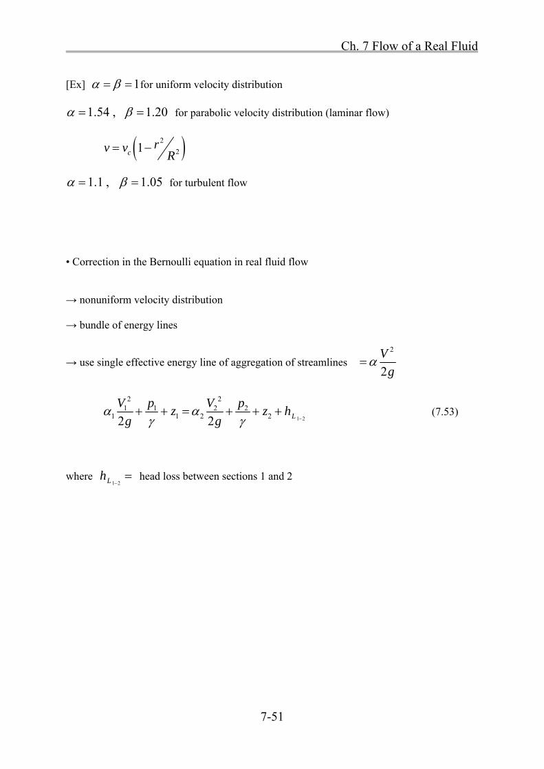
[Ex] 1 for uniform velocity distribution

1.54 , 1.20 for parabolic velocity distribution (laminar flow)

2

21crv v

R

1.1 , 1.05 for turbulent flow

• Correction in the Bernoulli equation in real fluid flow

→ nonuniform velocity distribution

→ bundle of energy lines

→ use single effective energy line of aggregation of streamlines 2

2

V

g

1 2

2 21 1 2 2

1 1 2 22 2 L

V p V pz z h

g g

(7.53)

where 1 2Lh head loss between sections 1 and 2


7-52

Homework Assignment # 7

Due: 1 week from today

Prob. 7.1

Prob. 7.7

Prob. 7.12

Prob. 7.17

Prob. 7.52

Prob. 7.58

Prob. 7.69

Chapter 7 Flow of a Real Fluid - Seoul National University

Documents

Transcript of Chapter 7 Flow of a Real Fluid - Seoul National University