Chapter 7: A Synthesizable VHDL Coding of a Genetic …ebrary.free.fr/Genetic Algorithms...

Chapter 7 A Synthesizable VHDL Coding of a Genetic Algorithm

Stephen D. Scott, Sharad Seth, and Ashok Samal

Abstract

This chapter presents the HGA, a genetic algorithm written in VHDL and intended for a hardware implementation. Due to pipelining, parallelization, and no function call overhead, a hardware GA yields a significant speedup over a software GA, which is especially useful when the GA is used for real-time applications, e.g. disk scheduling and image registration. Since a general-purpose GA requires that the fitness function be easily changed, the hardware implementation must exploit the reprogrammability of certain types of field-programmable gate arrays (FPGAs), which are programmed via a bit pattern stored in a static RAM and are thus easily reconfigured.

After presenting some background on VHDL, this chapter takes the reader through the HGA's code. We then describe some applications of the HGA that are feasible given the state-of-the-art in FPGA technology and summarize some possible extensions of the design. Finally, we review some other work in hardware-based Gas.

7.1. Introduction

This chapter presents the HGA, a genetic algorithm written in VHDL1 and intended for a hardware implementation. Due to pipelining, parallelization, and no function call overhead, a hardware GA yields a significant speedup over a software GA, which is especially useful when the GA is used for real-time applications, e.g. disk scheduling [51] and image registration [52]. Since a general-purpose GA requires that the fitness function be easily changed, the hardware implementation must exploit the reprogrammability of certain types of field-programmable gate

1VHDL stands for VHSIC (Very High Speed Integrated Circuit) Hardware Description Language.

©1999 by CRC Press LLC

arrays (FPGAs) [13], e.g. those from Xilinx [57]. Xilinx's FPGAs are programmed via a bit pattern stored in a static RAM and are thus easily reconfigured. While FPGAs are not as fast as typical application-specific integrated circuits (ASICs), they still hold a great speed advantage over functions executing in software. In fact, speedups of 1--2 orders of magnitude have been observed when frequently used software routines were implemented with FPGAs [8], [9], [12], [15], [19], [54]. Characteristically, these systems identify simple operations that are bottlenecks in software and map them to hardware. This is the approach used in this chapter, except that the entire GA is intended for a hardware implementation.

The remainder of this chapter is organized as follows. Section 7.2 gives a brief primer on VHDL. Section 7.3 describes the HGA design. Then in Section 7.4 we describe some applications of the HGA which are feasible given current FPGA technology. Possible design improvements and extensions are summarized in Section 7.5. Finally, in Section 7.6 we summarize and review other hardware-based Gas.

Also available are simulation results, a theoretical analysis of this design, and a description of a proof-of-concept prototype. They are beyond the scope of this chapter and are instead given in an associated technical report [44]. As they become available, updates to the code in this chapter will be made available at ftp://ftp.cse.unl.edu/pub/HGA.

Finally, it is important to distinguish hardware-based GAs from evolvable hardware. The former (e.g. the design presented in this chapter) is an implementation of a genetic algorithm in hardware. The latter involves using GAs and other evolution-based strategies to generate hardware designs that implement specific functions. In this case, each population member represents a hardware design, and the goal is to find an optimal design with respect to an objective function, e.g. how well the design performs a specific task. There are many examples of evolvable hardware in the literature [1], [17], [26], [43].

7.2. A VHDL Primer

In this section we briefly review some of the VHDL fundamentals employed in this chapter. Much more detail is available at the


ftp://ftp.cse.unl.edu/pub/HGA

VIUF and VHDLUK WWW sites [2], [3], which include lists of several VHDL books. The material in this section should be sufficient to allow the reader to comprehend the code of the design.

7.2.1. Entities, Architectures and Processes

Each module in the HGA consists of an ENTITY and an ARCHITECTURE. The entity portion of the module defines the PORT, which gives the data type, size and direction of all the inputs and outputs. For example, in the file fitness.hdl, ain is an input (due to the keyword IN), is of type qsim_state_vector (see below) and is n bits wide1, with the (n-1)th bit the most significant and the 0th bit the least significant (due to the keyword DOWNTO).

The architecture portion of a module defines its structure (specifying the interconnections between lower-level modules) or functionality (specifying what a module outputs in response to its inputs). In most of the VHDL files in this design, the architecture is specified behaviorally, and each architecture is composed of one or more PROCESSes. Typically the only process in each file is called main, but sometimes other processes exist, e.g. fitness.hdl also contains a process called adder which adds two values. Each process has a list of signals (signals are defined later) that it is sensitive to. When the value of any signal in the list changes, that process is activated. For example in fitness.hdl, if addval1 or addval2 changes, then process adder is activated and adds its inputs. If clk or init changes, then process main is activated.

7.2.2. Finite State Machines

Within the main process of each HGA module, a finite state machine with asynchronous reset is defined. Revisiting the example of fitness.hdl, the process main is activated by a change in clk (the system clock) and init (an asynchronous reset signal). The statement IF init='0' is true if the state machine has been reset, so in this part of the code the module shuts itself down. If instead init is 1, then regular state machine execution should proceed. The line

1n and other quantities are defined in Section 7.3.2.


ELSIF (clk'EVENT AND clk='1' AND clk'LAST_VALUE='0') THEN

is true only if init is 1, the clock has just changed (clk'EVENT), and the change was a low-to-high transition, i.e. the state machine only responds to positive clock edges, thus the machine's registers are all positive edge-triggered. If this ELSIF passes, we enter a CASE statement, in which we determine what state the machine is in and take the actions specified in that state. The names of the states are specified in the TYPE states IS . . . statement and a signal of type states is defined to hold the current state.

7.2.3. Data Types

Designs in VHDL manipulate SIGNALs and VARIABLEs. Signals are used to store states of state machines, communicate between modules, and communicate between different processes within the same module. Hence they are defined globally for an entire architecture or specified in a port. Variables can be defined locally for a single process. Signals can be thought of as sending information to other modules or processes, and variables can be thought of as storing information in a register. Another difference between signals and variables is that signals can have delays associated with them (e.g. propagation delay of a wire), to better resemble reality, whereas variables can not. Hence it is possible to examine the waveform of a signal but not of a variable. Assignment to a signal uses the<= operator and assignment to a variable uses the := operator.

The data types that variables and signals can assume include integer, bit, bit_vector, and user-defined data types. Type bit is a simple bit and can take on the values 0 and 1, so a signal of type bit is like a wire and a variable of type bit is like a flip-flop. Type bit_vector is an array of bits with a user-specified width, so a signal of type bit_vectoris like a bus and a variable of type bit_vector is like a register. In this design, we use the types qsim_state and qsim_state_vector, which are specific to the simulators and compilers of Mentor Graphics [33]. These types are nearly identical to bit and bit_vector, so a direct substitution should work to map the code of this chapter to code compatible with other VHDL compilers.

The functions to_qsim_state and to_integer appear frequently


in the code. The function to_integer(q) converts q, a qsim_state_vector, to an integer1. The function to_qsim_state(i,s) converts integer i to a qsim_state_vector that is s bits wide. These functions are used when adding qsim_state_vectors, using a qsim_state_vector as an index into an array, and to resize a qsim_state_vector. If the types qsim_state and qsim_state_vector are changed (e.g. to bit and bit_vector) for compatibility reasons, equivalent functions for to_qsim_state and to_integer must be written unless the equivalents already exist.

7.2.4. Miscellany

The LIBRARY and USE commands at the top of each VHDL file tells the VHDL compiler which libraries are used in that file. This design uses the mgc_portable library, which defines the typesqsim_state and qsim_state_vector as well as the functions to_integer and to_qsim_state. Our code also uses the libs.sizing library that is described in the file libs/sizing.hdl. In that file are several constants that parameterize the HGA design (Section 7.3.2).

Finally, note that all the VHDL code except that which is in memory.hdl is synthesizable. That is, it uses a subset of VHDL that can not only be simulated, but can be mapped to actual hardware by using AutoLogic II from Mentor Graphics [34], [35]. Other synthesizers exist and can be used to synthesize the HGA code if the Mentor-specific code is changed.

7.3. The Design

The functional model of the HGA is as follows. A software front end running on a PC or workstation interfaces with the user and writes the GA parameters (Section 7.3.1) into a memory that is shared with the back end, consisting of the HGA hardware. Additionally, the user specifies the fitness function in some

1Since these functions assume that q is in 2's complement form, a 0 bit is prepended to q before passing it to to_integer. This is done by using the & operator, which performs concatenation.


programming or other specification language (e.g. C or VHDL). Then software translates the specification into a hardware image and programs the FPGAs that implement the fitness function. Many such software-to-hardware translators exist [27], [35], [54]. Then the front end signals the back end. When the HGA back end detects the signal, it runs the GA based on the parameters in the shared memory. When done, the back end signals the front end. The front end then reads the final population from the shared memory. The population could then be written to a file for the user to view or have other computations performed on it. Currently the only GA termination condition that the user can specify is the number of generations to run. If other termination conditions are desired (e.g. amount of population diversity, minimum average fitness), the user must tell the HGA to run for a fixed number of generations and then check the resultant population to see if it satisfies the termination criteria. If not, then that population can be retained in the HGA's memory for another run. This process repeats until the termination criteria are satisfied.

Note that the front end could in fact be any interface between the HGA and a (possibly autonomous) system that occasionally requires the use of a GA. This system would select its own HGA parameters and initial population, give them to the front end for writing to the shared memory, and invoke the HGA. The system could even program the FPGAs containing the fitness function.

7.3.1. The User-Controlled (Run-Time) Parameters

The run-time parameters specified by the HGA's user are as follows. Their addresses in the shared memory are specified in libs/sizing.hdl (Section 7.3.2).

1. The number of members in the population. This is stored as psize in sequencer.hdl and as psize in fitness.hdl.

2. The initial seed for the pseudorandom number generator. This is stored as rn in rng.hdl, but is later overwritten with new random bit strings.

3. The mutation probability. This is stored as mutprob in xovermut.hdl.


4. The crossover probability. This is stored as xoverprob in xovermut.hdl.

5. The sum of the fitnesses of the members of the initial population. This is stored as sum in fitness.hdl, but is later overwritten with new sums as the population changes.

6. The number of generations in the HGA run. This is stored as numgens in fitness.hdl.

The initial population is stored in memory below the above parameters.

In directory makepop is C source code that will take GA parameters on the command line and create a file that includes these parameters plus a randomly generated population. The format of this file is directly readable by memory.hdl (Section 7.3.5.2) and thus can be immediately used as input when simulating the VHDL code of this chapter.

Other GA parameters such as the length of the population members1 and their encoding scheme are indirectly specified when the user defines the fitness function.

7.3.2. The VHDL Compile-Time Parameters

Designing the HGA using VHDL allowed the design to be specified behaviorally rather than structurally. It also allowed for general (parameter-independent) designs to be created, facilitating scaling. The specific designs implemented from the general designs depend upon parameters provided at VHDL compile time. When the parameters are specified, the design can be simulated or implemented with a VHDL synthesizer such as AutoLogic II from Mentor Graphics [34], [35]. The parameters are set in libs/sizing.hdl and used in the other VHDL files. They are as follows.

1. The width in bits of the crossover and mutation probabilities and the random numbers sent from rng.hdl to xovermut.hdl is denoted p.

1The maximum member size is specified in Section 7.3.2, but the actual length as interpreted by the fitness function could be less.


2. The maximum width in bits of the population members is denoted n.

3. The maximum width in bits of the fitness values is denoted f.

4. The precision used in scaling down the sum of fitnesses for selection in selection.hdl is denoted r. See Section 7.3.5.5 for more information.

5. The size of the cellular automaton in rng.hdl is denoted casize. See Section 7.3.5.1 for more information.

6. The maximum size of the population is denoted m.

7. The maximum number of generations is denoted maxnumgens.

8. The number of parallel selection modules is denoted nsel. Note: when changing nsel, the actual number of selection modules in top.hdl must also be changed.

The other constants defined in libs/sizing.hdl depend entirely on the above parameters, e.g. logn is the base-2 logarithm of n. Thus these constants are not discussed here.

The last portion of libs/sizing.hdl gives the locations in memory of the user-specified parameters described in Section 7.3.1.

7.3.3. The Architecture

The HGA (Figure 7.1) was based on Goldberg's simple genetic algorithm (SGA) [20]. The HGA's modules were designed to correlate well with the SGA's operations, be simple and easily scalable, and have interfaces that facilitate parallelization. They were also designed to operate concurrently, yielding a coarse-grained pipeline. The basic functionality of the HGA design is as follows1.

1. After loading the parameters into the shared memory, the front end signals the memory interface and control module (MIC, meminterface.hdl). The MIC acts as the main control unit of the HGA during start-up and shut-down and

1Note that Figure 7.1 shows only the data path; control lines are omitted.


is the HGA's sole interface to the outside world. After start-up and before shut-down, control is distributed; all modules operate autonomously and asynchronously.

2. The MIC notifies the fitness module (FM, fitness.hdl), crossover/mutation module (CMM, xovermut.hdl), the pseudorandom number generator (RNG, rng.hdl) and the population sequencer (PS, sequencer.hdl) that the HGA is to begin execution. Each of these modules requests its required user-specified parameters (Section 7.3.1) from the MIC, which fetches them from the shared memory.

3. The PS starts the pipeline by requesting population members from the MIC and passing them along to the selection module (SM, selection.hdl).

4. The task of the SM is to receive new members from the PS and judge them until a pair of sufficiently fit members is found. At that time it passes the pair to the CMM, resets itself, and restarts the selection process.

5. When the CMM receives a selected pair of members from the SM, it decides whether to perform crossover and mutation based on random values sent from the RNG. When done, the new members are sent to the FM for evaluation.

6. The FM evaluates the two new members from the CMM and writes the new members and their fitnesses to memory via the MIC. The FM also maintains information about the current state of the HGA that is used by the SM to select new members and by the FM to determine when the HGA is finished.

7. The above steps continue until the FM determines that the current HGA run is finished. It then notifies the MIC of completion which in turn shuts down the HGA modules and signals the front end.


Figure 7.1 The data path of the HGA architecture.

7.3.4. Inter-Module Communication

The modules in Figure 7.1 communicate via a simple asynchronous handshaking protocol similar to asynchronous bus protocols used in computer architectures [24]. When transferring data from the initiating module I to the participating module P, I signals P by raising a request signal to 1 and awaits an acknowledgment. When P agrees to participate in the transfer, it raises an acknowledgment signal. When I receives the acknowledgment, it sends to P the data to be transferred and lowers its request, signaling P that the information was sent. When P receives the data, it no longer needs to interact with I, so P lowers its acknowledgment. This signals I that the information was received. Now the transfer is complete and I and P are free to continue processing. Examples of this kind of transfer occur between the SM and CMM, between the CMM and FM, and between the FM and MIC.

When the HGA first starts up, all the modules except the SM issue requests to the MIC for the values of some of the user-specified parameters of Section 7.3.1. The communication protocol used is similar to that stated above. In this case, P is the MIC. After the MIC raises the acknowledgment, I sends the address of the parameter to read from memory. After the MIC reads the parameter from memory and sends it to I, the MIC lowers its acknowledgment. This same protocol is used when the PS reads population members from memory via the MIC.

7.3.5. Component Modules

In this section we describe in more detail the functionality of each


module from Figure 7.1.

7.3.5.1. Pseudorandom Number Generator (RNG)

The output of the pseudorandom number generator (RNG, rng.hdl) is used by two HGA modules. The RNG supplies pseudorandom bit strings (randsel1 and randsel2) to the selection module (SM, Section 7.3.5.5) for scaling down the sum of fitnesses. This scaled sum is used when selecting pairs of members from the population. The RNG also supplies pseudorandom bit strings to the crossover/mutation module (CMM, Section 7.3.5.6) for determining whether to perform crossover and mutation (doxover and domut) and what the crossover and mutation points are (xoverpt and mutpt).

After loading its seed into rn, the RNG uses a linear cellular automaton (CA) to generate a sequence of pseudorandom bit strings. The CA used in the RNG consists of 16 alternating cells which change their states according to rules 90 and 150 as described by Wolfram [56]:

Rule 90: s s si i i+

− += ⊕1 1

Rule 150: . s s s si i i i+

− += ⊕ ⊕1 1

Here is the current state of site (cell) in the linear array, is

the next state for , and is the exclusive OR operator. Serra et

al. [45] showed that a 16-cell CA whose cells are updated by the rule sequence 150-150-90-150 ... 90-150 produces a maximum-length cycle, i.e. it cycles through all possible bit patterns except the all 0s pattern. It has also been shown that such a rule sequence has more randomness than a linear feedback shift register

si i

16

si+

si ⊕

2

1 (LFSR) of corresponding length [28]. This scheme is implemented in state active in rng.hdl.

7.3.5.2. Shared Memory

The shared memory is actually external to the HGA system, but is

1LFSRs are commonly used as pseudorandom number generators in hardware.


presented here for completeness. The memory's specifications are known by the memory interface and control module (MIC, Section 7.3.5.3). It is shared by the back end and front end, acting as their primary communication medium. Before the HGA run, the front end writes the GA parameters of Section 7.3.1 into the memory and signals the MIC. When the HGA run is finished, the memory holds the final population which is then read by the front end.

Since an off-the-shelf physical memory would likely be employed in a hardware GA system, the file memory.hdl is intended for simulation purposes only. It reads its initial contents from a text file1. It is designed to behave like a real, but simple, memory. The memory only operates when the chip select (cs) and memory access (memacc) lines are low. When both these signals are low, if output enable (oe) is low, the memory outputs to dataout the value stored at address. If the read-write (rw) signal is low, then the memory stores into storage at address the value given in datain.

For tracking the progress of the simulation, memory.hdl maintains a variable called pulsecount that counts the total number of clock cycles in the run. It periodically writes this value to a file so the user can observe the rate of simulation. After the HGA shuts down, the memory writes its final contents (including the final population) to a text file, followed by the final value of pulsecount.

7.3.5.3. Memory Interface and Control Module (MIC)

The memory interface and control module (MIC, meminterface.hdl) is the only module in the HGA system which has knowledge of the HGA's environment. It provides a transparent interface to the memory for the rest of the system. When the MIC senses that go went low (state start1) and then high (state start2), it takes control of the shared memory2 by setting memacc to 0, initializes the other modules by setting init to 1, and begins

1This file can be created by makepop. See Section 7.3.1. 2At this point the MIC assumes that the front end has surrendered control of the memory.


to field requests from the other modules by transitioning to state idle.

The IF-ELSIF structure of state idle imposes priorities over the signals the MIC responds to. First it checks if fitdone is 1, indicating that the GA run has completed. If this is true, then it shuts down the other modules by setting init to 0, tells the user which population in memory is the final one by passing NOT toggle to toggleout1, relinquishes control of the memory by setting memacc to 1, and tells the front end that the HGA is finished by setting done to 1.

If instead fitdone is 0, then the MIC serves any outstanding requests from the other modules for user-specified parameters (Section 7.3.1). It does this by checking the signals reqrng through reqfit(0) in the order that they appear in meminterface.hdl. If any of these signals is high, then the MIC reads the appropriate parameter from memory by converting the address it receivesaddress understood by the memory. After reading the parameter from memory using a procedure described below, it (in state read2) sends the value out via valout and informs the module that the parameter was sent by setting all the acknowledgment signals to 0.

2 to an

The final cases covered by the IF-ELSIF structure of state idle are the ones most frequently encountered during normal HGA operation. If the signal reqfit(1) is 1 then the MIC knows that the fitness module (FM, Section 7.3.5.7) has a new population member to write to memory. The memory holds two populations, the current one and the new one (the new population will be the current one in the next generation). The FM writes to the new one and the population sequencer (PS, Section 7.3.5.4) reads from the current one. In state fit1, the MIC checks toggle, which the FM uses to inform the MIC which population is the new one. The MIC usestoggle to determine which base address (pop0base or pop1base) to add to the address sent from the FM (addrfit) to create the address sent to memory (address). It then takes the

1See Section 7.3.5.7. 2Which is as specified in libs/sizing.hdl.


value (valfitin) from the FM and writes it to memory.

If reqfit(1) is 0, then the MIC checks reqseq(1) to determine if the PS wants to read a new member from memory. If so, then in state seq1 the MIC checks toggle and builds address as above, using the opposite population as used by the FM. Then it reads the member from memory and passes it along to the PS via valout.

To read from memory, first the MIC transmits address to the memory, then enters state read1. During the state transition time (a single clock cycle), it is expected that the address has reached the input pins of the memory chip. So in read1 the MIC lowers oe, telling the memory it wants to read the data stored at the given address. After another clock cycle, the MIC enters read2, at which time it is expected that the data has arrived at datain. So the MIC forwards the data via valout, raises oe, and lowers the acknowledgments, indicating that it has forwarded the data.

The job of the population sequencer (PS, sequencer.hdl) is to cycle through the current population and pass the members on to the SM(s). After loading the population size into psize, the PS enters state getmember1, where it sends the index membaddr of a population member to the MIC via addr. Then it awaits reception of the member (arriving via value) in state getmember2. It then

To write to memory, first the MIC transmits address and dataout to the memory, then enters state write1. During the state transition time (a single clock cycle), it is expected that the address and data have reached the input pins of the memory chip. So in write1 the MIC lowers rw, telling the memory it wants to write the given data to the location given by the address. After another clock cycle, the MIC enters write2, at which time it is expected that the data has been written. So it raises rw, but keeps address and dataout unchanged so as to avoid corrupting memory. After one more clock cycle (the transition to write3), the MIC assumes the write was successful and informs the FM1.

7.3.5.4. Population Sequencer (PS)

1The FM is the only one informed here because it is the only module that writes data.


passes this member to the SM(s) via output. If the member sent to the SM(s) is the same as the previous one sent, dup is set to tell the SM(s) to accept it. The index membaddr is then incremented modulo the population size psize so the next population member will be requested from the MIC. This process continues until the GA run is complete and the MIC shuts down all the modules (i.e. init goes low).

7.3.5.5. Selection Module (SM)

The HGA's selection method is similar to the implementation of roulette wheel selection used in Goldberg's SGA [20]. The SGA's selection procedure is as follows.

1. Using a random real number r [0,1], scale down the sum of the fitnesses of the current population to get Sscale = r ξ Sfit.

2. Starting at the first population member, examine the members in the order they appear in the population.

3. Each time a new member is examined, accumulate its sum in a running sum of fitnesses SR. If at that time SR 3 Sscale, then the member under examination is selected. Otherwise the next population member is examined (Step 2).

Each time a new population member is to be selected, the above process is executed.

The selection module (SM, selection.hdl) implements the roulette wheel selection process used by the SGA, but it selects a pair of population members simultaneously rather than a single member at a time. First, from the FM it receives sum, the sum of the fitnesses of the current population. It then scales down this sum by two random values rand1 and rand2 provided by the RNG. The actual scaling is performed in the process scalefit which multiplies an r-bit random bit string by the sum of fitnesses and then right shifts the result by r bits (Section 7.3.2). This is done to simplify the division operation in the hardware. Thus larger values ofr yield more precision in scaling down sum. Since a multiplier that operates in a single clock cycle consumes a significant amount of hardware, only one is instantiated in the SM. So in state init1 the variables serialize and multdone are used to coordinate the


two accesses to process scalefit. The two scaled sums are stored in scalea and scaleb. After storing the scaled sums, the SM resets the fitness accumulators accuma and accumb, the members a and b and the flags donea and doneb. Now selection may begin.

The state getcandidates is where selection is performed. First the flags donea and doneb are checked. If either of these is 1, then the corresponding member (e.g. a if donea = 1) is not changed because the done flag indicates that it has already been selected. So any member with a done flag = 0 is replaced by input when a new member arrives1. After storing a new input into a and/or b, serialize is set to 1 to indicate that the running sums of fitnesses accuma and accumb require updating, since new members were stored. Then the SM checks if accuma > scalea. If so, then a has been selected and the SM sets donea to 1. doneb is set to 1 under similar conditions. When both donea and doneb are 1, the SM moves to state awaitackxover1 and transmits a and b to the CMM via the handshaking protocol described in Section 7.3.4. Then the SM returns to state init1 to select another member. Finally, note that the reset signal comes from the FM to indicate that the current generation has ended and the FM has switched the population it writes to (Sections 7.3.5.3 and 7.3.5.7). Thus the PS now reads from a different population. This means that sum is no longer the sum of the fitnesses of the current population. So a reset places the SM into state idle where it stores the new sof into sum and restarts selection.

The HGA is designed to allow for multiple SMs to operate in parallel, which is useful when the SM is the bottleneck of the pipeline [44]. The PS sends the same members to all SMs, but this does not pose a problem for selection since each SM uses an independent pair of random bit strings to scale down the sum of fitnesses. Thus each selection process is independent of the others. All the parallel SMs feed into a single CMM. To add parallel SMs, nsel in libs/sizing.hdl must be changed, and alterations are necessary in top.hdl (Section 7.3.6).

1A new member's arrival is indicated by a change in input or if dup is 1 (Section 7.3.5.4).


7.3.5.6. Crossover/Mutation Module (CMM)

After loading values into mutprob and xoverprob, the crossover/mutation module (CMM, xovermut.hdl) remains in state findreqsel while polling the SM(s). When SM i has selected members, it sends a request. When the index currsel = i, the CMM will detect SM i's request and accept the pair of members via the handshaking protocol of Section 7.3.4, storing them in a1 and b1. Then if the random string doxover (from the RNG, Section 7.3.5.1) is smaller than the crossover probability xoverprob, crossover is performed while copying a1 into a2 and b1 into b2, where the crossover point is indicated by xoverpt. Then a2 is copied into a3 and b2 into b3, where the bit of a2 indexed by mutpt is mutated if domut < mutprob. Then the CMM acknowledges the SM so it may start a new selection process. Finally, the CMM transmits the new members a3 and b3 to the FM via the handshaking protocol of Section 7.3.4 and resumes polling the SMs.

Note that the HGA only has one opportunity per pair of members to perform mutation, but in Goldberg's SGA, the possibility of mutation is explored for every bit of every member. Thus the SGA's mutation probability is effectively higher than the one used in the HGA. This can be adjusted for by increasing the mutation probability given to the HGA or by a few simple alterations to xovermut.hdl to make the HGA's mutation operator the same as the SGA's.

7.3.5.7. Fitness Module (FM)

When the fitness module (FM, fitness.hdl) starts up, it loads toggleinit into tog, which tells the FM which of the two populations contains the initial one specified by the user. Then the FM stores the population size in psize, stores the sum of fitnesses of the initial population in sum(0) or sum(1), depending on the value of tog, and stores the number of generations in numgens.

After initializing, the FM enters state newgen to start a new


generation1. It first checks if the entire HGA run is over (if numgens = 0). If not, it resets psizetmp (the number of population members remaining to fill the current generation) and sof(NOT tog) (the sum of fitnesses accumulator for the new generation). It also toggles tog and sends its value to the MIC via toggle, which tells the MIC which population the FM writes to and which the PS reads from. Finally, it sends a 0 to the SM via reset, which tells the SM that the sum of fitnesses of the population the SM reads from has been updated. Then the FM moves to waitforxovreq, where it awaits a new pair of members from the CMM.

In waitforxovreq, the FM first checks if psizetmp = 0, indicating the end of the current generation. Otherwise the FM awaits a request from the CMM and then receives a and b via ain and bin using the handshaking protocol of Section 7.3.4. For evaluating a and b, the FM can use its default fitness function of , distributed over states waitforxovreq2 and sumfitb. Alternatively, an optional external fitness evaluator (FE) can be attached to the FM. If it is attached, then offchipfit will be 1, causing the FM to senda and b, one at a time, to the FE via offchipfitmemb and receive each member's fitness via offchipfitres. These actions occur in states offchipfita and offchipfitb. After each member is evaluated (in either the FM or FE), the FM accumulates the sum of their fitnesses in sum(NOT tog) by using the process adder, which implements a single adder in the FM. After the current generation completes, sum(NOT tog) will be sent to the SM.

f x x( ) = 2

In the current design, the FM expects the FE to evaluate each member in a single clock cycle. But this restriction can be removed by implementing a slightly more complex communication protocol

1The flag cleanxover is used to insert a delay before the FM starts a new generation. This is necessary because of a small technicality: if the CMM was processing members from the old population when the FM switched populations (due to the new generation), then the FM should ignore the CMM's output. The use of ackxover and cleanxover in states newgen and waitforxovreq achieves this goal.


between the FM and FE. Use of an external FE allows all the other HGA modules (including the FM, which would now only perform bookkeeping) to be implemented in a non-reprogrammable technology such as fabricated chips, to reap a space and time savings over FPGAs. Only the FE need be implemented on reprogrammable FPGAs. Additionally, since the implementation of the FE is independent of the FM's implementation, the FE could be implemented in software if the fitness function is much too complex for an FPGA implementation. All that is required is that the software-based FE adhere to the communication protocol expected by the FM.

After evaluating the new members and accumulating their fitnesses, the FM uses the handshaking protocol of Section 7.3.4 to send the members and their fitnesses to the MIC for writing to memory.

While not in the current design, it is possible to allow for multiple FMs to operate in parallel, much like the parallel SMs of Section 7.3.5.5. This is useful when the FM is the bottleneck of the pipeline [44]. If parallel FMs were to be added to this design, the duty of writing new members to memory and maintaining records of the HGA's state (e.g. maintaining numgens and psizetmp) would best be shifted from the FM to a new module called the memory writer (MW). This is because maintaining these values in a distributed fashion would be difficult. The CMM would connect to all the FMs, and each FM would connect to the MW.

To add parallel FMs, an MW should be created, the FM should be modified, and a parameter nfit in libs/sizing.hdl should be added. Also, alterations would be necessary in top.hdl.

7.3.6. Combining the Modules

The file top.hdl specifies the connections between all the modules and the HGA's interface to its environment. The entity top defines the HGA's interface and the COMPONENT definitions describe the interfaces of each HGA module. Below the COMPONENT definitions are the definitions of signals that interconnect the modules. Each signal is explained by comments in the code. The next portion of top.hdl defines which VHDL source file corresponds with each component. This is where multiple SMs are instantiated, if desired.


Finally, the components are interconnected by specifying which signals connect to each component. Naturally, the size and type of each signal must match the size and type of the port it connects to. Also, multiply-driven signals are disallowed unless some arbitration logic is utilized, so in top.hdl, exactly one port connected to each signal is an OUT port, which can be seen in the COMPONENT definitions.

Note that the instantiation of the mem component (for memory) implies that as written, top.hdl is intended for simulation only. In fact, the file top.hdl might not be used at all in an actual implementation since groups of components will likely be mapped to different FPGAs.

7.4. Example Applications

This section gives a high-level description of several problems that the HGA is applicable to given the current state-of-the-art in FPGA technology.

7.4.1. A Mathematical Function

Our first example application comes from Michalewicz [36]. The problem is to optimize the function

f x x x x x x( , ) . sin( ) sin( )1 2 1 1 2 2215 4 20= + +π π (1)

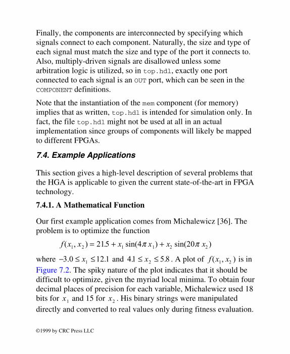
where and . A plot of is in Figure 7.2. The spiky nature of the plot indicates that it should be difficult to optimize, given the myriad local minima. To obtain four decimal places of precision for each variable, Michalewicz used 18 bits for and 15 for . His binary strings were manipulated directly and converted to real values only during fitness evaluation.

− ≤ ≤3 0 12 11. .x

x1 x

41 5 82. ≤ ≤x . f x x( , )1 2

2


Figure 7.2 Plot of Equation 1, the function f x x( ,1 2 ) .

A hardware implementation of this fitness function is straightforward if the CORDIC algorithm [53] is used to evaluate the sines. To evaluate Equation 1 in hardware, we require a single multiplier1, two adder/subtracters, six registers, two shifters, and a lookup table in the form of a 16 ROM. All these components easily fit on a Xilinx XC4013 FPGA [57].

18×

In the evaluation process, first is multiplied by x1 4π in the

multiplier, and then is multiplied by x2 20π in the multiplier in the next cycle. Then both sine calculations run concurrently via CORDIC. But since CORDIC only works on arguments between 0 and 2π , before running CORDIC we must subtract from each argument to sine an amount 2iπ , where )2i x= / ( π for

x x{4 x∈ ,20 }1 2π π . These amounts are 1x2 2π and 2 10 2π x ,

1Since multipliers occupy significant FPGA space and can reduce the maximum possible clock rate, a dedicated multiplier chip, such as the AMD Am29323 multiplier [5], could be used instead. This would increase the maximum possible clock rate and save area on the FPGAs.


each of which is computable with two more uses of the multiplier1. So after four cycles, one of the two concurrent CORDIC systems is given an argument of 4 2 21π πx −

2x

0 24 13− − −< <)1

1x . After another three cycles,

the other CORDIC system receives an argument of . Fourteen steps of each CORDIC are required

to attain 4 decimal places of precision in the result, which is the precision used in Michalewicz's implementation. Fourteen steps are required because approximately one bit of accuracy is attained in each step, and . After the first CORDIC finishes, multiply by sin(

20 2 102π πx −

14

x1 42 1

π x and add the result to 21.5. One cycle after this, the second CORDIC will finish. So multiply by x2

sin( )20 2π x and add this result to x x1 14 2) .15sin( π + . By overlapping as many operations as possible while sharing the multiplier and adder, the total time to evaluate the member is 23 cycles. Now repeat for the other member, yielding a cumulative delay of 46 cycles. But note that operations performed in evaluating the first member can partially overlap operations evaluating the second. So in fact, both members can be evaluated in 43 cycles.

iπjπ from x for j

1For arbitrary x 3 0, 2repeatedly subtracting 2

can be found with a binary search, ranging from

In related work [44], we give simulation results on this problem and contrast the results to those from a software implementation of Goldberg's SGA.

7.4.2. Logic Partitioning

Sitkoff et al. [46] have proposed a scheme to apply GAs to the

log ( / )2 x πput j in a set Sx and continue. W

down to 1. After each subtraction, if the result 3 0, and continue. If the result < 0, then add 2jπ back to

hen finished,. 2 2i j

j S

π π=∈∑ . If initially x < 0,

a sim jπ to x and test hen finished,

then performif the result is < 0. W

ilar process, but repeatedly add 2π 2 j

j S∈∑ yields a quantity

and 0. Now add 2πbetween -2π to this quantity.


problem of partitioning logic designs across two FPGAs. A design is comprised of c components and a particular partitioning (population member) is represented by a c-bit string P, where the ith bit is 1 if and only if component i lies in FPGA 1. Accompanying this bit string is a set of c-bit strings Nj, one per inter-component net in the design, where the ith bit of Nj is 1 if and only if component i is connected to Nj. So net j lies in FPGA 1 of partition P if one of the bits in P Nj is 1, where is the bitwise AND operator. Likewise, net j lies in FPGA 2 of partition P if one of the bits in ~P Nj is 1, where ~P is the bitwise not of P. Thus, a net j crosses a chip boundary if and only if some bit from P Nj is 1 and some bit from ~P Nj is 1. This can easily be determined with combinational logic. A partition's fitness is then the total number of boundary crossings. This fitness function can easily be evaluated in hardware, just like in Sitkoff et al.'s work. The nets Nj used to evaluate each P are the same for each P, so they can be permanently stored in the FM. Since the number of potential nets is exponential in c, the nets Nj might need to be stored in some memory attached to the FM.

This approach can be generalized to an arbitrary (but bounded) number of FPGAs F as follows (Figure 7.3). First store P in c registers, each with bits. Each register represents which

of the F FPGAs its corresponding component lies in. Then for each net Nj, a counter initializes itself to 0 and cycles through all integer values v [0, F]. For each value v, compare it to Pi (the index of the FPGA holding component i) for all i. If they are equal, then component i lies in FPGA v in partition P. Now logically AND this result with the ith bit of Nj. If this result is 1, then Nj lies at least in part on FPGA v. The results for all i are logically ORed yielding a single bit indicating if Nj lies in FPGA v. This result is fed into an accumulator which counts the number of FPGAs that Nj lies in. After looping through all values of v [0, F], the accumulator is checked. If it holds a value >1, then Nj crosses a chip boundary. Repeat this process for all Nj. The fitness of P is as defined before.

log2 F


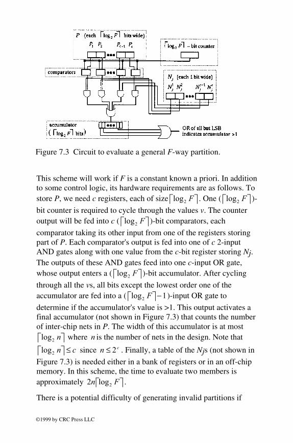
Figure 7.3 Circuit to evaluate a general F-way partition.

This scheme will work if F is a constant known a priori. In addition to some control logic, its hardware requirements are as follows. To store P, we need c registers, each of size log2 F . One ( log2 F )-

bit counter is required to cycle through the values v. The counter output will be fed into c ( log2 F )-bit comparators, each

comparator taking its other input from one of the registers storing part of P. Each comparator's output is fed into one of c 2-input AND gates along with one value from the c-bit register storing Nj. The outputs of these AND gates feed into one c-input OR gate, whose output enters a ( log2 F )-bit accumulator. After cycling

through all the vs, all bits except the lowest order one of the accumulator are fed into a ( 1−log2 F

)-input OR gate to

determine if the accumulator's value is >1. This output activates a final accumulator (not shown in Figure 7.3) that counts the number of inter-chip nets in P. The width of this accumulator is at most

where is the number of nets in the design. Note that

since . Finally, a table of the Njs (not shown in

Figure 7.3) is needed either in a bank of registers or in an off-chip memory. In this scheme, the time to evaluate two members is approximately .

log2 n

log2 n

cn

2

≤ n ≤

2log

c2

n F

There is a potential difficulty of generating invalid partitions if


bitwise crossover and mutation are used when . This is because a value could appear in Pi that is > F, defining an invalid partition. This can be remedied by requiring that the initial population be valid, crossover respects the boundaries between bit groups, and that mutation only maps a bit group into a valid bit group.

F F< 2 2log

Finally, note that given the net specification of a circuit, the set of vectors Nj and the fitness evaluation hardware can be automatically generated by software. So the user's work can be limited to specifying the components and nets of the circuit.

7.4.3. Hypergraph Partitioning

A GA approach to the hypergraph partitioning problem by Chan and Mazumder [16] uses a fitness function similar to that described in Section 7.4.2. After counting the number of nets that span the partition, this value is divided by the product of the sizes of the two partitions. This is known as the ratio cut cost and only involves a little extra work (the multiplication and division operations) beyond what is done in Section 7.4.2. Thus the HGA is applicable to this problem. Also, as in Section 7.4.2, the fitness function can be generalized to F-way partitioning where F is arbitrary but known a priori.

7.4.4. Test Vector Generation

When fabricating VLSI chips, occasionally the process introduces faults into the chip, causing incorrect functionality. Thus it is desirable to detect the faulty chips before packaging and shipping them to customers. Since the chip testers typically only have access to the inputs and outputs of the chip (not the internal structure), the only way to detect faults is by applying a test vector to the inputs and then contrast the output with the expected output (i.e. the output that would be produced by a fault-free circuit). If they differ, then the chip is faulty and is rejected. If they do not differ, then the other test vectors are applied. If the chip passes all the tests, the chip is accepted. The goal is to generate the smallest set of test vectors that still detects most (or all) possible faults in the chip.

In this section we focus on the single stuck-at fault model. In this


model any faulty circuit has only a single fault, and the fault is of the following form: some wire in the circuit is permanently stuck at 0 (e.g. the wire is short-circuited to ground) or 1 (e.g. the wire is short-circuited to power). See Abramovici et al. [4] for more information on this and other fault models.

O'Dare and Arslan [38] have described a GA to generate test vectors for stuck-at fault detection in combinational circuits (i.e. circuits with no memory). In their scheme, each population member is a single test vector. The member's fitness is evaluated on the basis of how many new faults it covers. The GA maintains a global table which defines the current set of vectors. A vector is added to the table if it covers a fault not already covered by another vector in the table. Using a software-based fault simulator, each vector is evaluated by first applying it to a fault-free version of the circuit under test (CUT). Then each node within the CUT is in turn forced to a logic 1 and a logic 0 to simulate the stuck-at faults. If the circuit's output differs from the fault-free output, then the vector detects the given fault. Each vector gets a fixed number of points for each fault it covers that is not already covered by the test set, and it receives a smaller number of points for each fault it covers that is already covered.

We now propose how to map O'Dare and Arslan's fitness function to hardware for the HGA. Each logic gate in the CUT is mapped to a pair of gates that allow simulation of stuck-at faults. Figure 7.4 gives an example of this for an AND gate. To simulate the output c as stuck at 0, both x and y are set to 0. To simulate c stuck at 1, x is set to 0 and y is set to 1. To simulate fault-free behavior, x is set to 1 and y is set to 0. OR and NOT gates and the original inputs can be modified in a similar fashion. For a circuit with n gates and m inputs, the new circuit has at most 2n + 2m gates and at most 2n + 2m extra inputs that are controlled by the fitness module. This hardware-based fault simulation component of our proposed hardware implementation of O'Dare and Arslan's fitness function is similar to hardware accelerators designed for fault simulation [29], [58] and logic simulation [14], [39], [47].


Figure 7.4 An example of mapping a logic gate to a stuck-at fault simulation gate.

Then fitness evaluation simply requires a look-up table of previously selected vectors and the faults that they cover, a counter to cycle through all 2(m+n) possible stuck-at faults, an accumulator for the members' scores, and some simple control logic. The time to evaluate a member is approximately the number of faults plus one, so the time to evaluate two members is about 4(m+n)+2. Finally, the mapping process from the original circuit to the fitness evaluation hardware can be automated as in Section 7.4.2, relieving the user of that responsibility.

7.4.5. Traveling Salesman and Related Problems

Here we consider GA approaches to the traveling salesman problem (TSP), which poses special difficulties. Using a straightforward encoding consisting of a permutation of cities encounters problems if conventional crossover and mutation operators are used. This is because regular (or uniform) crossover, if it changes anything, will create two invalid tours, i.e. some cities will appear more than once and some will not appear at all. Thus much work in applying GAs to the TSP (e.g. [20], [22]) involve the use of special crossover operators that preserve the validity of tours. This method can be used in the HGA but requires modification of the CMM. In lieu of this, conventional crossover operators can be used in conjunction with a special encoding of the population members. One such encoding is called a random keys encoding [11], [37]. In this encoding, each tour is represented by a tuple of random numbers, one number for each city, with each number from [0,1]. After selecting a pair of tours, simple or uniform crossover can be applied, yielding two new tuples. To evaluate these tuples, sort the numbers and visit the cities in ascending order of the sort. For example, in a five-city problem the tuple (0.52,0.93,0.26,0.07,0.78) represents the tour 4 ♦ 3 ♦ 1 ♦ 5♦ 2. This tour can then be evaluated. Note that every tuple maps to a valid tour, so any crossover scheme is applicable.


When employing this scheme, all that is required of the HGA's FM is, upon receiving a population member, to sort the tuple and accumulate the distances between the cities of the tour. Sorting of the numbers can be done with a sorting circuit based on the Odd-Even Merge Sort algorithm [10]1. For sorting numbers (i.e. for

-city tours), the depth of the sorting network is

. Each level of the network has

registers and comparators

n

) 2

)

n

(log log /2 2 1 2n n +n / 2

n / 2log

( )log log2 2 1n n +

)

n2. Also, a single set of registers

and comparators can simulate the sorting network using some

finite state logic and steps. Thus the

hardware requirements of the FM include some finite state logic, a linear number of registers and comparators, and a lookup table that provides the inter-city distances (with entries). In this case, the time to evaluate two members is approximately

.

n

( log /2 2 1n n +

O n( 2

Finally, we note that the scheme just presented can be adapted for application to other problems with similar constraints as the TSP. These include scheduling problems, vehicle routing, and resource allocation (a generalization of the 0-1 knapsack problem and the set partitioning problem) [11], [37]. The HGA can be applied to these problems as well with a slight increase in complexity.

7.4.6. Other NP-Complete Problems

In this section we explore the exploitation of polynomial-time reductions between instances of NP-complete problems. Developing a GA to solve any NP-complete problem (e.g. SAT, the boolean satisfiability problem) yields automatic solutions to all other NP-complete problems via the reductions. All that is required is to (in software) map the instance of any NP-complete problem to SAT, apply the SAT (hardware-based) GA to solve it, and then (in

1Also see an excellent description by Leighton [30]. 2The size of each register and comparator depends on the desired precision of the numbers in the tuples, but should be at least log2 n bits.


software) map the SAT solution to a solution of the original problem. Of course, the GA must find an optimal solution (i.e. a satisfying assignment for a SAT instance) for this to work. A fit member in the SAT GA may map to a worthless non-solution in another problem unless the SAT member is optimal.

The idea of exploiting the reductions between NP-complete problems was studied extensively by DeJong and Spears [18], who also provided a SAT GA and empirical results on the hamiltonian circuit (HC) problem. Their SAT GA evaluates a population member by quantifying how "close'' the bit string is to satisfying the given boolean function . They do this by assigning a numeric value to each expression in and combining them. Specifically, given boolean expressions , the fitness value of ,

denoted , is given as follows for the operators AND ( ),

OR ( ) and NOT (~):

ff1e e

x

, ,K l ei

val ei( ) ∧∨

, val e e avg val e val e( ) ( ( ), , ( ))1 1∧ ∧ =L Kl l

, val e e val e val e( ) max( ( ), , ( ))1 1∨ ∨ =L Kl l

and

, val e val ei i(~ ) ( )= −1

where returns the mean of the values . An

example of these evaluation functions appears in Table 7.1. Notice in the table that an assignment has a fitness of 1.0 if and only if it satisfies . This is true in general if satisfies some simple conditions

avg x x( , , )1 K l

f

x1, ,K l

f1. While improvements to these evaluation functions

were suggested, empirically those described above performed well in the work of DeJong and Spears and are simple enough for a hardware implementation.

1These conditions are not listed here, but any boolean formula can be made to satisfy them with only a linear increase in its size.


x x val f x x avg x x xavgavgavgavg

1 2 1 2 1 1 210 0 1 0 0 0 0 50 1 1 0 0 1 1 01 0 1 1 1 0 0 51 1 1 1 11 0 5

( ( , )) ( , max( , ))( , max( , )) .( , max( , )) .( , max( , )) .( , max( , )) .

= −− =− =− =− =

A hardware GA implementation for the SAT GA could work as follows. Take the given boolean formula and map it to a circuit consisting of AND, OR and NOT gates where each AND and OR gate has only two inputs. Then replace each inverter in the circuit with a module that subtracts its input from the constant 1, replace each OR gate with a module that outputs the maximum of its two inputs, and replace each AND gate with a module that adds its two inputs and right shifts the result by one bit. The result is a circuit that outputs the fitness of the input binary string. The number of gates in the new circuit is more than in the old circuit by only a linear factor of the precision (number of bits) used to represent the fitnesses. Thus an HGA implementation of the SAT GA is feasible.

f

7.5. Extensions of the Design

There are many possible ways to extend the design of Section 7.3, many of which require only simple modifications to the VHDL code. First, other genetic algorithm operators could be implemented, including uniform crossover [48], multi-point crossover, and inversion [20]. Permutation-preserving crossover and mutation operators [20], [22] could be implemented for constrained problems such as the TSP. Additionally, the CMM could be parameterized to respect the boundaries of bit groups, i.e. only permit crossover at certain locations. This would be useful in preventing invalid strings in the generalized FPGA partitioning (Section 7.4.2) and hypergraph partitioning (Section 7.4.3) problems. Also, other selection methods [21] could be implemented. When implemented, these methods would be made available to the user via the software front end. The user would select the desired selection and crossover methods as HGA parameters. Also recall from Section 7.3 that if other GA termination conditions are desired besides running for a fixed number of generations (e.g. amount of population diversity, minimum average fitness), the front end can

e

x

)Table 7.1: Evaluating assignments for and in the SAT GA

when attempting to satisfy

x1

~x2

x( 1f x x x x( , )1 2 1 2= ∧ ∨ .


tell the HGA to run for a fixed number of generations and then check the resultant population to see if it satisfies the termination criteria. If not, then that population is retained in the HGA's memory for another run. This process repeats until the termination criteria are satisfied.

Another extension of this design involves allowing parallelization of the fitness modules. This is useful when the pipeline's bottleneck lies in the FM rather than the SM [44]. As mentioned in Section 7.3.5.7, a new module called the memory writer (MW) would be very useful for arbitrating memory writes and performing bookkeeping functions, e.g. maintaining the values numgens and psizetmp.

To extend the parallelization of the system, the SM-CMM-FM pipeline could be parallelized by replicating the highlighted portion (dotted box) of Figure 7.1. As with the parallel FM configuration mentioned above, an MW would be useful in this scheme. Other improvements include merging the PS with the MIC and changing the handshaking protocol of Section 7.3.4 to take fewer clock cycles. These reductions of communication delay should improve performance.

If the population members are extremely large (e.g. hundreds or thousands of bits), then it is unrealistic to send entire members between modules in parallel. Instead the modules could process data in stream form, where processing begins when the first few bits arrive in the module and output begins while input and processing still occur. That is, the result of processing the first portion of input is sent to the next module before the rest of the input arrives. So the members travel in a "cut-through'' fashion through each module rather than the "store-and-forward'' fashion of Section 7.3. In the stream model, the SM operates on members' addresses and fitnesses rather than on the members themselves and their fitnesses. Once a pair of members is selected, the SM tells the CMM the addresses of the selected members. The CMM then fetches these members from memory and begins sending them to the FM, performing crossover and mutation while it transmits. If fitness function evaluation can begin before receiving the entire member, then as it evaluates the member, the FM begins to write it into memory before evaluation or input is complete. If this is not


possible, then multiple passes over the members is necessary for evaluation, so on-chip buffers are required.

7.6. Summary and Related Work

This chapter described the HGA, a general-purpose VHDL-based genetic algorithm intended for a hardware implementation. The design is parameterized, facilitating scaling. It is possible to implement the HGA on reprogrammable FPGAs, exploiting the speed of hardware while retaining the flexibility of a software implementation. The result is a general-purpose GA engine which is useful in many applications where software-based GA implementations are too slow, e.g. when real-time constraints apply.

Recently there has been more work on hardware-based GAs. Other VHDL GA implementations include Alander et al. [6] and Graham and Nelson [22]. Salami and Cain applied the design of this chapter to the problems of finding optimal gains for a proportional integral differential (PID) controller [41] and optimization of electricity generation in response to demand [42]. Additionally, Tommiska and Vuori [49] implemented a GA with Altera HDL (AHDL) for implementation on Altera FLEX 10K FPGAs [7].

A subset of the GA operations have been mapped to hardware by Liu [31], who designed and simulated a hardware implementation of the crossover and mutation operators. In similar work, Red'ko et al. [40] developed a GA which implemented crossover and mutation in hardware. Hesser et al. [25] implemented in hardware crossover, mutation, and a simple neighborhood-based selection routine. Hämäläinen et al. [23] designed the genetic algorithm parallel accelerator (GAPA), which is a tree structure of processors for executing a GA. The GAPA is a parallel GA with specialized hardware support to accelerate certain operations. Sitkoff et al. [46] designed a hardware GA for partitioning logic designs across Xilinx FPGAs. After running the GA in software, the bottleneck was determined to be in evaluation of the fitness function. Thus parallel fitness evaluation modules were implemented on FPGAs and the remainder of the GA ran in software. Megson and Bland [32] present a design for a hardware-based GA that implements all the GA operations except fitness evaluation in a pipeline of seven


systolic arrays.

Problem-specific (non-FPGA) implementations include a suite of proprietary GAs in a text compression chip from DCP Research Corporation [55]. Other examples include Turton et al.'s applications to image processing [50], image registration [52], disk scheduling [51], and Chan et al.'s application to hypergraph partitioning [16]. These GAs were designed for implementation on VLSI chips and thus are neither reconfigurable nor general-purpose. They are also expensive to produce in small quantities. However, the intended applications are popular, so a VLSI implementation seems justifiable since the systems can be produced in bulk.

References

[1] Darwin on a chip. The Economist, page 85, February 1993.

[2] VHDL International Users Forum (VIUF), 1997. http://www.vhdl.org/viuf.

[3] VHDLUK: A communication network for VHDL users, 1997 http://www.vhdluk.org/.

[4] M. Abramovici, M. A. Breuer, and A. D. Friedman. Digital Systems Testing and Testable Design. AT&T Bell Laboratories and W. H. Freeman and Company, New York, New York, 1990.

[5] Advanced Micro Devices. Bipolar Microprocessor and Logic Interface (Am29000 Family) Data Book, 1985. http://www.amd.com/.

[6] J. T. Alander, M. Nordman, and H. Setälä. Register-level hardware design and simulation of a genetic algorithm using VHDL. In P. Osmera, editor, Proceedings of the 1st International Mendel Conference on Genetic Algorithms, Optimization, Fuzzy Logic and Neural Networks, pages 10--14, 1995.

[7] Altera Corporation, San Jose, California. Flex 10k Embedded Programmable Logic Family, 1996. http://www.altera.com/.

[8] J. M. Arnold, D. A. Buell, and E. G. Davis. Splash 2. In Proceedings of the 4th Annual ACM Symposium on Parallel Algorithms and Architectures, pages 316--324, June 1992.


http://www.vhdl.org/viuf

http://www.amd.com/

http://www.altera.com/

[9] P. M. Athanas and H. F. Silverman. Processor reconfiguration through instruction-set metamorphosis. IEEE Computer, 26(3):11--18, March 1993.

[10] K. Batcher. Sorting networks and their applications. In Proceedings of the AFIPS Spring Joint Computing Conference, volume 32, pages 307--314, 1968.

[11] J. Bean. Genetics and random keys for sequencing and optimization. ORSA Journal on Computing, 6:154--160, 1994.

[12] P. Bertin, D. Roncin, and J. Vuillemin. Programmable active memories: A performance assessment. In G. Borriello and C. Ebeling, editors, Research on Integrated Systems: Proceedings of the 1993 Symposium, pages 88--102, 1993.

[13] S. D. Brown, R. J. Francis, J. Rose, and Z. G. Vranesic. Field-Programmable Gate Arrays. Kluwer Academic Publishers, Boston, Massachusetts, 1992.

[14] C. Burns. An architecture for a Verilog hardware accelerator. In Proceedings of the IEEE International Verilog HDL Conference, pages 2--11, February 1996. http://www.crl.com/www/users/cb/cburns/.

[15] S. Casselman. Virtual computing and the virtual computer. In R. Werner and R. S. Sipple, editors, Proceedings of the IEEE Workshop on FPGAs for Custom Computing Machines, pages 43--48. IEEE Computer Society Press, April 1993. http://www.vcc.com/.

[16] H. Chan and P. Mazumder. A systolic architecture for high speed hypergraph partitioning using a genetic algorithm. In X. Yao, editor, Progress in Evolutionary Computation, pages 109--126, Berlin, 1995. Springer-Verlag. Lecture Notes in Computer Science number 956.

[17] H. de Garis. An artificial brain. New Generation Computing, 12:215--221, 1994.

[18] K. A. De Jong and W. M. Spears. Using genetic algorithms to solve NP-complete problems. In J. D. Schaffer, editor, Proceedings of the Third International Conference on Genetic Algorithms, pages 124--132. Morgan Kaufmann Publishers, Incorporated, June 1989.


http://www.vcc.com/

[19] M. Gokhale, W. Holmes, A. Kosper, S. Lucas, R. Minnich, D. Sweely, and D. Lopresti. Building and using a highly parallel programmable logic array. IEEE Computer, 24(1):81--89, January 1991.

[20] D. E. Goldberg. Genetic Algorithms in Search, Optimization, and Machine Learning. Addison-Wesley Publishing Company, Incorporated, Reading, Massachusetts, 1989.

[21] D. E. Goldberg and K. Deb. A comparative analysis of selection schemes used in genetic algorithms. In G. Rawlings, editor, Foundations of Genetic Algorithms, pages 69--93, 1991.

[22] P. Graham and B. Nelson. A hardware genetic algorithm for the traveling salesman problem on Splash 2. In 5th International Workshop on Field-Programmable Logic and its Applications, pages 352--361, August 1995. http://splish.ee.byu.edu/.

[23] T. Hämäläinen, H. Klapuri, J. Saarinen, P. Ojala, and K. Kaski. Accelerating genetic algorithm computation in tree shaped parallel computer. Journal of Systems Architecture, 42(1):19--36, August 1996.

[24] J. P. Hayes. Computer Architecture and Organization. McGraw-Hill Book Company, New York, second edition, 1989.

[25] J. Hesser, J. Ludvig, and R. Männer. Real-time optimization by hardware supported genetic algorithms. In P. Osmera, editor, Proceedings of the 2nd International Mendel Conference on Genetic Algorithms, Optimization, Fuzzy Logic and Neural Networks, pages 52--59, 1996.

[26] T. Higuchi, H. Iba, and B. Manderick. Evolvable hardware. In H. Kitano and J. A. Hendler, editors, Massively Parallel Artificial Intelligence, pages 398--421. MIT Press, 1994.

[27] H. Högl, A. Kugel, J. Ludvig, R. Männer, K.-H. Noffz, and R. Zoz. Enable++: A second generation FPGA processor. In Proceedings of the IEEE Symposium on FPGAs for Custom Computing Machines, pages 45--53, April 1995.

http://www-mp.informatik.uni-mannheim.de/.


http://splish.ee.byu.edu/

[28] P. D. Hortensius, H. C. Card, and R. D. McLeod. Parallel random number generation for VLSI using cellular automata. IEEE Transactions on Computers, 38:1466--1473, October 1989.

[29] S. Kang, Y. Hur, and S. A. Szygenda. A hardware accelerator for fault simulation utilizing a reconfigurable array architecture. VLSI Design, 4(2):119--133, 1996. http://www.ece.utexas.edu/ece/people/profs/Szygenda.ht

ml.

[30] F. T. Leighton. Introduction to Parallel Algorithms and Architectures: Arrays, Trees, Hypercubes. Morgan Kaufmann Publishers, Incorporated, San Mateo, California, 1992.

[31] J. Liu. A general purpose hardware implementation of genetic algorithms. Master's thesis, University of North Carolina at Charlotte, 1993.

[32] G. M. Megson and I. M. Bland. A generic systolic array for genetic algorithms. Technical report, University of Reading, May 1996. http://www.cs.rdg.ac.uk/cs/research/Publications/repor

ts.html.

[33] Mentor Graphics Corporation, Wilsonville, Oregon. Mentor Graphics VHDL Reference Manual, 1994. http://www.mentor.com/.

[34] Mentor Graphics Corporation, Wilsonville, Oregon. VHDL Style Guide for AutoLogic II, 1995. http://www.mentor.com/.

[35] Mentor Graphics Corporation, Wilsonville, Oregon. Synthesizing with AutoLogic II, 1996. http://www.mentor.com/.

[36] Z. Michalewicz. Genetic Algorithms + Data Structures = Evolution Programs. Springer-Verlag, Berlin, second edition, 1994.

[37] B. Norman and J. Bean. Random keys genetic algorithm for job shop scheduling. Engineering Design and Automation, to appear.

http://www-personal.engin.umich.edu/~jbean/.


http://www.cs.rdg.ac.uk/cstr/

http://www.mentor.com/



http://www-personal.engin.umich.edu/~jbean/

[38] M. J. O'Dare and T. Arslan. Hierarchical test pattern generation using a genetic algorithm with a dynamic global reference table. In Proceedings of the First IEE/IEEE International Conference on Genetic Algorithms in Engineering Systems: Innovations and Applications, pages 517--523, September 1995. http://vlsi2.elsy.cf.ac.uk/group/.

[39] Precedence, Incorporated, Campbell, California. Product Brief, 1996. http://www.precedence.com/.

[40] V. G. Red'ko, M. I. Dyabin, V. M. Elagin, N. G. Karpinskii, A. I. Polovyanyuk, V. A. Serechenko, and O. V. Urgant. On microelectronic implementation of an evolutionary optimizer. Russian Microelectronics, 24(3):182--185, 1995. Translated from Mikroelektronika, vol. 24, no. 3, pp. 207--210, 1995.

[41] M. Salami and G. Cain. An adaptive PID controller based on a genetic algorithm processor. In Proceedings of the First IEE/IEEE International Conference on Genetic Algorithms in Engineering Systems: Innovations and Applications, pages 88--93, September 1995.

[42] M. Salami and G. Cain. Multiple genetic algorithm processor for the economic power dispatch problem. In Proceedings of the First IEE/IEEE International Conference on Genetic Algorithms in Engineering Systems: Innovations and Applications, pages 188--193, September 1995.

[43] E. Sanchez and M. Tomassini, editors. Towards Evolvable Hardware: The Evolutionary Engineering Approach. Springer-Verlag, Berlin, 1996. Lecture Notes in Computer Science number 1062.

[44] S. D. Scott, S. Seth, and A. Samal. A hardware engine for genetic algorithms. Technical Report UNL-CSE-97-001, University of Nebraska-Lincoln, July 1997. ftp://ftp.cse.unl.edu/pub/TechReps/UNL-CSE-97-001.ps.gz.

[45] M. Serra, T. Slater, J. C. Muzio, and D. M. Miller. The analysis of one-dimensional linear cellular automata and their aliasing properties. IEEE Transactions on Computer-Aided Design of Integrated Circuits and Systems, 9(7):767--778, July 1990.


[46] N. Sitkoff, M. Wazlowski, A. Smith, and H. Silverman. Implementing a genetic algorithm on a parallel custom computing machine. In IEEE Symposium on FPGAs for Custom Computing Machines, pages 180--187, April 1995. http://www.lems.brown.edu/arm/.

[47] Synopsys, Incorporated, Mountain View, California. ARKOS Datasheet, 1997. http://www.synopsys.com/.

[48] G. Syswerda. Uniform crossover in genetic algorithms. In Proceedings of the Third International Conference on Genetic Algorithms and their Applications, pages 2--9, 1989.

[49] M. Tommiska and J. Vuori. Implementation of genetic algorithms with programmable logic devices. In J. T. Alander, editor, Proceedings of the Second Nordic Workshop on Genetic Algorithms and their Applications (2NWGA), pages 71--78, August 1996. http://www.uwasa.fi/cs/publications/2NWGA.html.

[50] B. C. H. Turton and T. Arslan. An architecture for enhancing image processing via parallel genetic algorithms & data compression. In Proceedings of the First IEE/IEEE International Conference on Genetic Algorithms in Engineering Systems: Innovations and Applications, pages 337--342, September 1995. http://vlsi2.elsy.cf.ac.uk/group/.

[51] B. C. H. Turton and T. Arslan. A parallel genetic VLSI architecture for combinatorial real-time applications---disc scheduling. In Proceedings of the First IEE/IEEE International Conference on Genetic Algorithms in Engineering Systems: Innovations and Applications, pages 493--499, September 1995. http://vlsi2.elsy.cf.ac.uk/group/.

[52] B. C. H. Turton, T. Arslan, and D. H. Horrocks. A hardware architecture for a parallel genetic algorithm for image registration. In Proceedings of the IEE Colloquium on Genetic Algorithms in Image Processing and Vision, pages 11/1--11/6, October 1994. http://vlsi2.elsy.cf.ac.uk/group/.

[53] J. E. Volder. The CORDIC trigonometric computing technique. IRE Transactions on Electronic Computers, EC-8:330--334, September 1959.


http://www.lems.brown.edu/arm/

http://www.synopsys.com/

http://www.uwasa.fi/cs/publications/2NWGA/2NWGA.html

[54] M. Wazlowski, A. Smith, R. Citro, and H. F. Silverman. Armstrong III: A loosely-coupled parallel processor with reconfigurable computing capabilities. Technical report, Brown University, 1996. http://www.lems.brown.edu/arm/.

[55] L. Wirbel. Compression chip is first to use genetic algorithms. Electronic Engineering Times, page 17, December 1992.

[56] S. Wolfram. Universality and complexity in cellular automata. Physica, 10D:1--35, 1984.

[57] Xilinx, Incorporated, San Jose, California. The Programmable Logic Data Book, 1996. http://www.xilinx.com/.

[58] Zycad Corporation, Fremont, California. Paradigm XP Product News, 1996. http://www.zycad.com/.


http://www.lems.brown.edu/arm/

http://www.xilinx.com/

Chapter 7: A Synthesizable VHDL Coding of a Genetic …ebrary.free.fr/Genetic Algorithms...

Documents

Transcript of Chapter 7: A Synthesizable VHDL Coding of a Genetic …ebrary.free.fr/Genetic Algorithms...