Chapter 6

Operant Conditioning Schedules

Schedule of Reinforcement

• Appetitive outcome --> reinforcement– As a “shorthand” we call the appetitive

outcome the “reinforcer”– Assume that we’ve got something appetitive

and motivating for each individual subject

• Fairly consistent patterns of behaviour

• Cumulative recorder

Cumulative Record

• Cumulative recorder

• Flat line

• Slope

paper strip

pen

roller roller

Cumulative Recorder

Recording Responses

The Accumulation of the Cumulative Record

VI-25

Fixed Ratio (FR)

• N responses required; e.g., FR 25• CRF = FR1• Rise-and-run• Postreinforcement pause• Ratio strain

Time

no responses

reinforcement

responses“pen” resetting

Variable Ratio (VR)• Varies around mean number of responses; e.g.,

VR 25

• Short, if any postreinforcement pause

• Never know which response will be reinforced

Fixed Interval (FI)

• Depends on time; e.g., FI 25

• Postreinforcement pause; scalloping

• Clock doesn’t start until reinforcer given

Variable Interval (VI)

• Varies around mean time; e.g., VI 25

• Don’t know when time has elapsed

• Clock doesn’t start until reinforcer given

Response Rates

FR 25 VR 25 FI 25 VI 25

75 50 25 VR FR VI FI Slope = rise run

Duration Schedules

• Continuous responding for some time period to receive reinforcement

• Fixed duration (FD)– Set time period

• Variable duration (VD)– Varies around a mean

Differential Rate Schedules

• Differential reinforcement of low rates (DRL)– Reinforcement only if X amount of time has passed

since last response– Sometimes “superstitious behaviours”

• Differential reinforcement of high rates (DRH)– Reinforcement only if more than X responses in a

set time

Noncontingent Schedules

• Reinforcement delivery not contingent upon passage of time

• Fixed time (FT)– After set time elapses

• Variable time (VT)– After variable time elapses

Choice Behaviour

Choice

• Two-key procedure

• Concurrent schedules of reinforcement

• Each key associated with separate schedule

• Distribution of time and behaviour

Concurrent Ratio Schedules

• Two ratio schedules

• Schedule that gives most rapid reinforcement chosen exclusively

Concurrent Interval Schedules

• Maximize reinforcement

• Must shift between alternatives

• Allows for study of choice behaviour

Interval Schedules

• FI-FI– Steady-state responding– Less useful/interesting

• VI-VI– Not steady-state responding– Respond to both alternatives– Sensitive to rate of reinforcemenet– Most commonly used to study choice

Alternation and the Changeover Response

• Maximize reinforcers from both alternatives

• Frequent shifting becomes reinforcing– Simple alternation– “Concurrent superstition”

Changeover Delay

• COD

• Prevents rapid switching

• Time delay after “changeover” before reinforcement possible

Herrnstein’s (1961) Experiment

• Concurrent VI-VI schedules

• Overall rates of reinforcement held constant– 40 reinforcers/hour between two alternatives

Key Schedule Rft/hr Rsp/hr Rft rate Rsp rate1 VI-3min 20 2000 0.5 0.52 VI-3min 20 2000 0.5 0.5

1 VI-9 6.7 250 0.17 0.082 VI-1.8 33.3 3000 0.83 0.92

1 VI-1.5 40 4800 1.0 1.02 Extinction 0 0 0 0

1 VI-4.5 13.3 1750 0.33 0.312 VI-2.25 26.7 3900 0.67 0.69

Proportional Rate of ResponseB1 = resp. on key 1B2 = resp. on key 2

Proportional Rate of ReinforcementR1 = reinf. on key 1R2 = reinf. on key 2

R1

R1+R2

=

0.50.5

2020

B1

B1+B2

= 20002000+2000

= 0.5

0.50.5

20002000

2020+20

= 0.5 R1

R1+R2

= 6.76.7+33.3

= 0.17

0.17 0.83

6.733.3

0.080.92

2503000

B1

B1+B2

= 250250+3000

= 0.08

The Matching Law

• The proportion of responses directed toward one alternative should equal the proportion of reinforcers delivered by that alternative.

Bias

• Spend more time on one alternative than predicted

• Side preferences

• Biological predispositions

• Quality and amount

Varying Quality of Reinforcers

• Q1: quality of first reinforcer

• Q2: quality of second reinforcer

Varying Amount of Reinforcers

• A1: amount of first reinforcer

• A2: amount of second reinforcer

Combining Qualities and Amounts

Extinction

Extinction (Muted) TimeOut TimeOut TimeOut TimeOut TimeOut TimeOut

Extinction Extinction burst FR 1 (CRF)

Extinction

• Disrupt the three-term contingency

• Response rate decreases

Stretching the Ratio/Interval

• Increasing the number of responses• e.g., FR 5 --> FR 50, VI 4 sec. --> VI 30 sec.• Extinction problem• Shaping; gradual increments• “Low” or “high” schedules

Extinction

• Continuous Reinforcement (CRF) = FR 1• Intermittent schedule: everything else• CRF easier to extinguish than any intermittent

schedules• Partial reinforcement effect (PRE)• Generally:

– High vs. low– Variable vs. fixed

Discrimination Hypothesis

• Difficult to discriminate between extinction and intermittent schedule

• High schedules more like extinction than low schedules

• e.g., CRF vs. FR 50

Frustration Hypothesis

• Non-reinforcement for response is frustrating• On CRF every response reinforced; no frustration• Intermittent schedules always have some non-

reinforced responses– Responding leads to reinforcer (pos. reinf.)

– Frustration = S+ for reinforcement

• Frustration grows continually during extinction– Stop responding --> stops frustration (neg. reinf.)

Sequential Hypothesis

• Response followed by reinf. or nonreinf.• Intermittent schedules: nonreinforced

responses are S+ for eventual delivery of reinforcer

• High schedules increase resistance to extinction because many nonreinforced responses in a row leads to reinforced

• Extinction similar to high schedule

Response Unit Hypothesis

• Think in terms of behavioural “units”

• FR1: 1 response = 1 unit --> reinforcement

• FR2: 2 responses = 1 unit --> reinforcement– Not “response-failure, response-reinforcer” but

“response-response-reinforcer”

• Says PRE is an artifact

Mowrer & Jones (1945)

• Response unit hypothesis

• More responses in extinction on higher schedules disappears when considered as behavioural units

300

250

200

150

100

50

Nu

mb

er o

f re

spon

ses/

un

its

du

rin

g ex

tin

ctio

n

FR1 FR2 FR3 FR4

absolute number of responses

number of behavioural units

Economic Concepts and Operant Behaviour

• Similarities

• Application of economic theories to behavioural conditions

The Economic Analogy

• Responses or time = money

• Total responses or time possible = income

• Schedule = price

Consumer Demand• Demand curve

– Price of something and how much is purchased– Elasticity of demand

Am

ount

Pur

chas

ed

Price

Elastic

Inelastic

Three Factors in Elasticity of Demand

• 1. Availability of substitutes– Can’t substitute complementary reinforcers

• e.g., food and water

– Can substitute non-complementary reinforcers• e.g., Coke and Pepsi

• 2. Price range– e.g., FR3 to FR5 vs. FR30 to FR50

• 3. Income level– Higher total response/time…the less effect cost

increases have– Increased income --> purchase luxury items– Shurtleff et al. (1987)

• Two VI schedules; food, saccharin water

• High schedules: rats spend most time on food lever

• Low schedules: rats increase time on saccharin lever

Behavioural Economics and Drug Abuse

• Addictive drugs• Nonhuman animal

models• Elasticity

– Work for drug reinforcer on FR schedule

– Inelastic...up to a point

low medium high very high

Price (FR schedule)R

espo

nse

rate

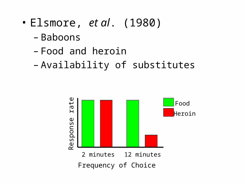
• Elsmore, et al. (1980)– Baboons– Food and heroin– Availability of substitutes

2 minutes 12 minutes

Frequency of Choice

Res

pons

e ra

te

Food

Heroin