Chapter 6:Modulation Techniques for Mobile Radio

School of Information Science and Engineering, SDU

Outlinel Frequency versus Amplitude Modulationl Amplitude Modulation (AM)l Angle Modulationl Digital Modulationl Line Codingl Pulse Shaping Techniquesl Geometric Representation of Modulation Signall Linear Modulation Techniquesl Constant Envelope Modulationl M-ary signaling

What is modulation

l Modulation is the process of encoding information from a message source in a manner suitable for transmission

l It involves translating a baseband messagesignal to a bandpass signal at frequencies that are very high compared to the baseband frequency.

l Baseband signal is called modulating signall Bandpass signal is called modulated signal

Modulation Techniquesl Modulation can be done by varying the l Amplitudel Phase, orl Frequency

of a high frequency carrier in accordance with the amplitude of the message signal.

l Demodulation is the inverse operation: extracting the baseband message from the carrier so that it may be processed at the receiver.

Analog/Digital Modulation

l Analog Modulation l The input is continues signall Used in first generation mobile radio systems

such as AMPS in USA. l Digital Modulationl The input is time sequence of symbols or pulses. l Are used in current and future mobile radio

systems

Goal of Modulation Techniques

l Modulation is difficult task given the hostile mobile radio channelsl Small-scale fading and multipath conditions.

l The goal of a modulation scheme is: l Transport the message signal through the radio

channel with best possible qualityl Occupy least amount of radio (RF) spectrum.

Frequency versus Amplitude Modulationl Frequency Modulation (FM)

l Most popular analog modulation techniquel Amplitude of the carrier signal is kept constant (constant envelope

signal), the frequency of carrier is changed according to the amplitude of the modulating message signal; Hence info is carried in the phase or frequency of the carrier.

l Has better noise immunity: § atmospheric or impulse noise cause rapid fluctuations in the amplitude of the received

signal

l Performs better in multipath environment§ Small-scale fading cause amplitude fluctuations as we have seen earlier.

l Can trade bandwidth occupancy for improved noise performance.§ Increasing the bandwith occupied increases the SNR ratio.

l The relationship between received power and quality is non-linear. § Rapid increase in quality for an increase in received power. § Resistant to co-channel interference (capture effect).

Frequency versus Amplitude Modulationl Amplitude Modulation (AM)l Changes the amplitude of the carrier signal

according to the amplitude of the message signal.l All info is carried in the amplitude of the carrierl There is a linear relationship between the received

signal quality and received signal power.l AM systems usually occupy less bandwidth then FM

systems. l AM carrier signal has time-varying envelope.

Amplitude Modulationl The amplitude of high-carrier signal is varied

according to the instantaneous amplitude of the modulating message signal m(t).

AM Modulatorm(t) sAM(t)

)2cos()](1[)()(

)2cos(

tftmAtstm

tfA

ccAM

cc

π

π

+=

:Signal AMThe

:Signal Message Modulating

:Signal Carrier

Modulation Index of AM Signal

c

m

AAk =

)2cos()( tfAtm mm π=For a sinusoidal message signal

Index is defined as:

SAM(t) can also be expressed as:

)](1()(})(Re{)( 2

tmAtgetgts

c

tfjAM

c

+==

where

π

g(t) is called the complex envelope of AM signal.

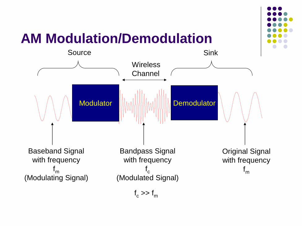
AM Modulation/Demodulation

Modulator Demodulator

Baseband Signalwith frequency

fm(Modulating Signal)

Bandpass Signalwith frequency

fc(Modulated Signal)

Wireless Channel

Original Signalwith frequency

fm

Source Sink

fc >> fm

AM Modulation - Example

-20

-15

-10

-5

0

5

10

15

20

0 2 4 6 8 10 12 14

)2cos()]cos(221[4)()2cos()](1[)(

)10cos(4)2cos()cos(22)(

tfttstftmAts

ttfAttm

cAM

ccAM

cc

ππ

π

++=+=

=+=

:Signal AM

: signal Carrier

:signal Message

Hzf

Hzf

mesg

c

16.021

6.1210

==

≅=

π

π

1/fmesg

1/fc

Angle Modulation

l Angle of the carrier is varied according to the amplitude of the modulating baseband signal.

l Two classes of angle modulation techniques: l Frequency Modulation

§ Instantaneous frequency of the carrier signal is varied linearly with message signal m(t)

l Phase Modulation§ The phase θ(t) of the carrier signal is varied linearly with the

message signal m(t).

Angle Modulation

+=+= ∫

∞−

t

fccccFM dxxmktfAttfAts )(22cos)](2cos()( ππθπ

kf is the frequency deviation constant (kHz/V)

If modulation signal is a sinusoid of amplitude Am, frequency fm:

)]2sin(2cos()( tffAk

tfAts mm

mfccFM ππ +=

[ ])(2cos)( tmktfAts ccPM θπ +=kθ is the phase deviation constant

PHASE MODULATION

FREQUENCY MODULATION

- + --

FM Example:

[ ])82cos(

)2sin(482cos)()2cos(4)(

tttts

ttm

πππ

π+=

=Message signal

FM Signal

Carrier Signal

0

-4

4

10.5 21.5

+

FM Index

Wf

WAk mf

f∆

==β

W: the maximum bandwidth of the modulating signal∆f: peak frequency deviation of the transmitter. Am: peak value of the modulating signal

Example: Given m(t) = 4cos(2π4x103t) as the message signal anda frequency deviation constant gain (kf) of 10kHz/V;Compute the peak frequency deviation and modulation index!

fm=4kHz

∆f = 10kHz/V * 4V = 40kHz.βf = 40kHz / 4kHz = 10

Answer:

Spectra and Bandwidth of FM Signals

mfT fB )1(2 += β

An FM Signal has 98% of the total transmitted power in a RF bandwidth BT

fBT ∆= 2 Lower bound

Upper bound

Example: Analog AMPS FM system uses modulation index of Bf = 3 and fm = 4kHz. Using Carson’s Rule: AMPS has 32kHz upper bound and 24kHz lower

bound on required channnel bandwidth.

Carson’s Rule

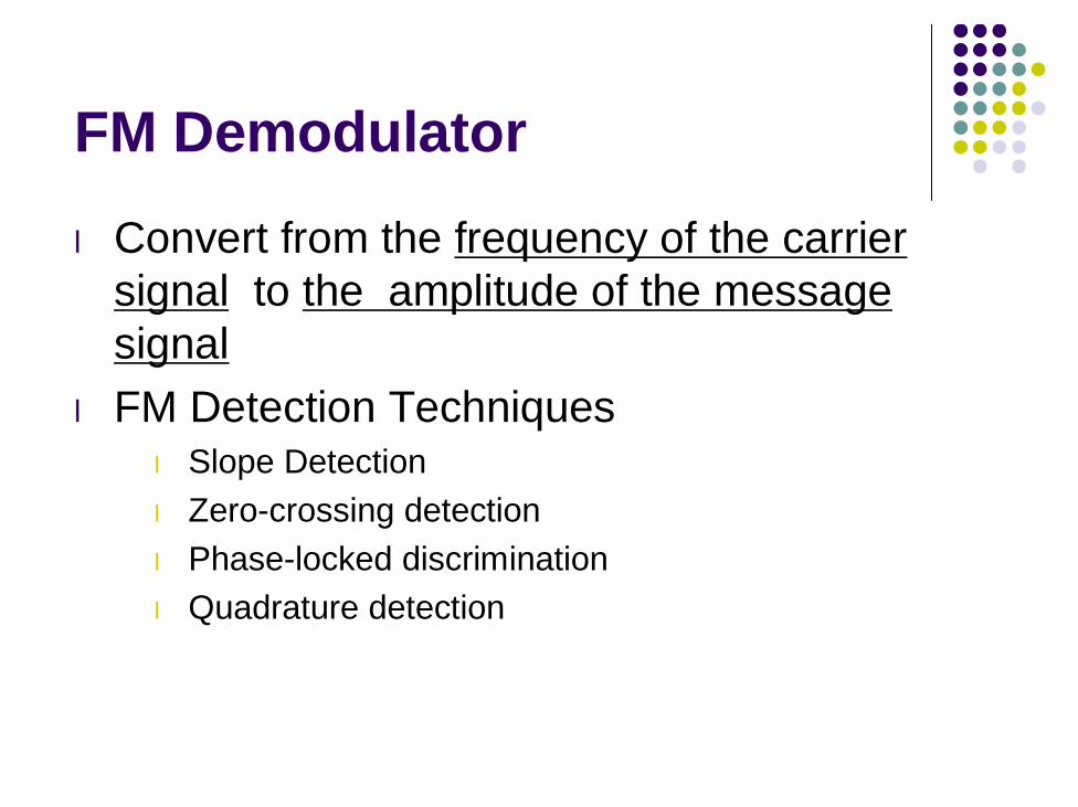
FM Demodulator

l Convert from the frequency of the carrier signal to the amplitude of the message signal

l FM Detection Techniquesl Slope Detectionl Zero-crossing detectionl Phase-locked discriminationl Quadrature detection

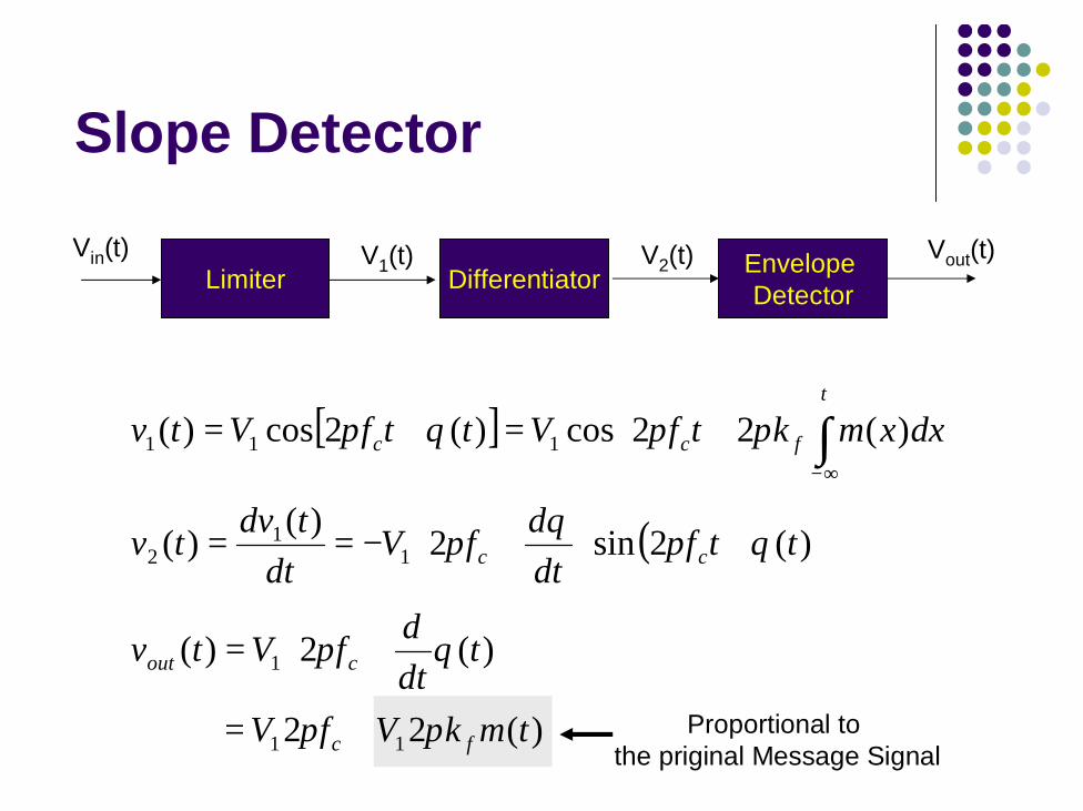
Slope Detector

[ ]

( )

)(22

)(2)(

)(2sin2)()(

)(22cos)(2cos)(

11

1

11

2

111

tmkVfV

tdtdfVtv

ttfdtdfV

dttdvtv

dxxmktfVttfVtv

fc

cout

cc

t

fcc

ππ

θπ

θπθ

π

ππθπ

+=

+=

+

+−==

+=+= ∫

∞−

Limiter Differentiator Envelope Detector

Vin(t) V1(t) V2(t) Vout(t)

Proportional to the priginal Message Signal

Digital Modulation

l The input is discrete signalsl Time sequence of pulses or symbols

l Offers many advantagesl Robustness to channel impairmentsl Easier multiplexing of variuous sources of information:

voice, data, video. l Can accommodate digital error-control codesl Enables encryption of the transferred signals

§ More secure link

Digital ModulationThe modulating signal is respresented as a time-sequence of symbolsor pulses.

Each symbol has m finite states: That means each symbol carries n bitsof information where n = log2m bits/symbol.

...0 1 2 3 T

One symbol(has m states – voltage levels)

(represents n = log2m bits of information)

Modulator

Factors that Influence Choice of Digital Modulation Techniques

l A desired modulation scheme l Provides low bit-error rates at low SNRs§ Power efficiecny

l Performs well in multipath and fading conditionsl Occupies minimum RF channel bandwidth§ Bandwidth efficieny

l Is easy and cost-effective to implement

l Depending on the demands of a particular system or application, tradeoffs are made when selecting a digital modulation scheme.

Power Efficiency of Modulationl Power efficiency is the ability of the modulation technique to

preserve fidelity of the message at low power levels. l Usually in order to obtain good fidelity, the signal power needs

to be increased.l Tradeoff between fidelity and signal powerl Power efficiency describes how efficient this tradeoff is made

= PER

NEb

p :Efficiency Power certain for input receiver the at required0

η

Eb: signal energy per bit N0: noise power spectral densityPER: probability of error

Bandwidth Efficiency of Modulation

l Ability of a modulation scheme to accommodate data within a limited bandwidth.

l Bandwidth efficiency reflect how efficiently the allocated bandwidth is utilized

bps/Hz :Efficiency BandwidthBR

B =η

R: the data rate (bps)B: bandwidth occupied by the modulated RF signal

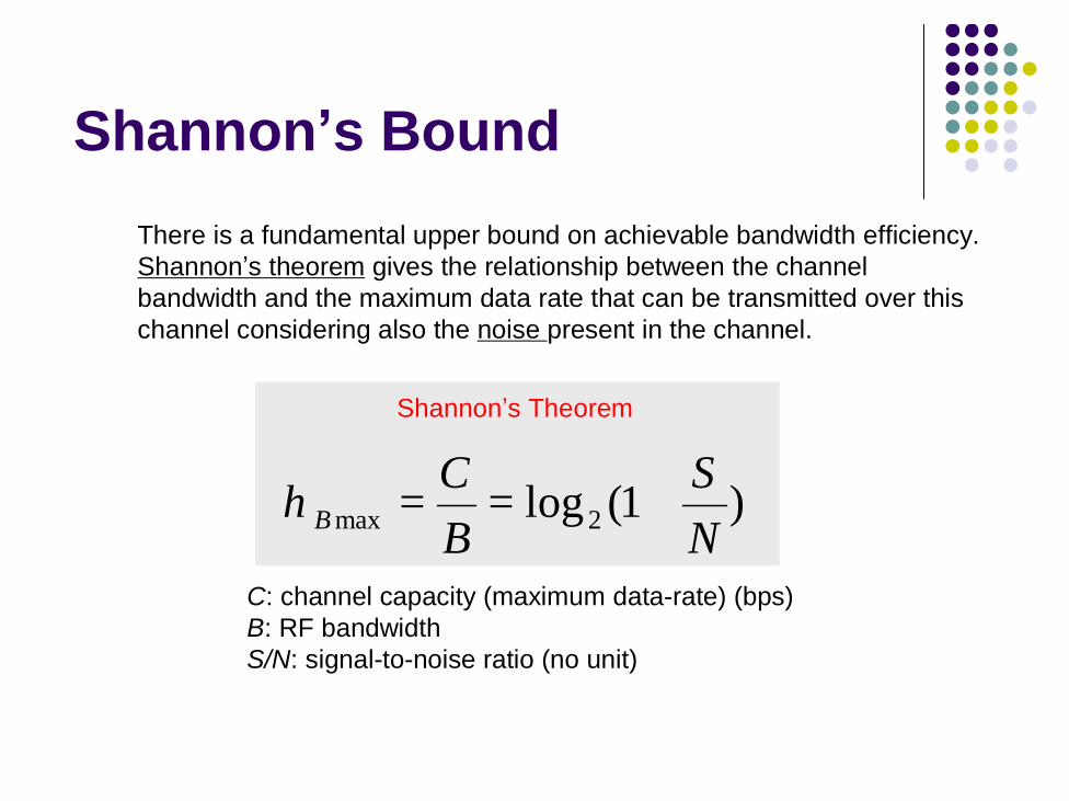
Shannon’s BoundThere is a fundamental upper bound on achievable bandwidth efficiency.Shannon’s theorem gives the relationship between the channel bandwidth and the maximum data rate that can be transmitted over this channel considering also the noise present in the channel.

)1(log 2max NS

BC

B +==η

Shannon’s Theorem

C: channel capacity (maximum data-rate) (bps)B: RF bandwidthS/N: signal-to-noise ratio (no unit)

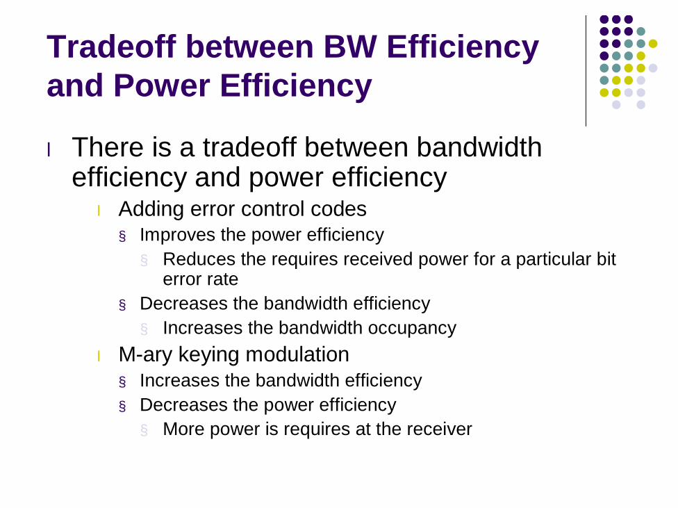
Tradeoff between BW Efficiency and Power Efficiency

l There is a tradeoff between bandwidth efficiency and power efficiencyl Adding error control codes§ Improves the power efficiency§ Reduces the requires received power for a particular bit

error rate§ Decreases the bandwidth efficiency§ Increases the bandwidth occupancy

l M-ary keying modulation§ Increases the bandwidth efficiency§ Decreases the power efficiency§ More power is requires at the receiver

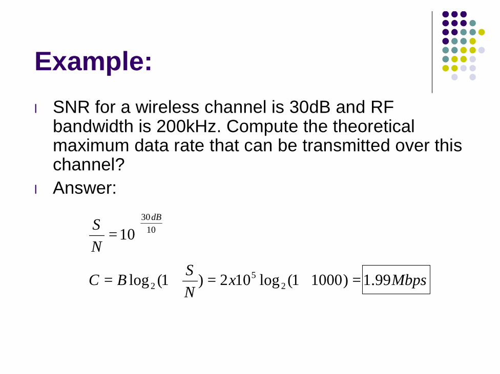
MbpsxNSBC

NS dB

99.1)10001(log102)1(log

10

25

2

1030

=+=+=

=

Example: l SNR for a wireless channel is 30dB and RF

bandwidth is 200kHz. Compute the theoretical maximum data rate that can be transmitted over this channel?

l Answer:

Noiseless Channels and NyquistTheorem

For a noiseless channel, Nyquist theorem gives the relationship between the channel bandwidth and maximum data rate that can betransmitted over this channel.

mBC 2log2=

Nyquist Theorem

C: channel capacity (bps)B: RF bandwidthm: number of finite states in a symbol of transmitted signal

Example: A noiseless channel with 3kHz bandwidth can only transmitmaximum of 6Kbps if the symbols are binary symbols.

Power Spectral Density (PSD) of Digital Signals and Bandwidth

l What does signal bandwidth mean? l Answer is based on Power Spectral Density (PSD)

of Signalsl For a random signal w(t), PSD is defined as:

<<−

=

=

∞→

elsewhere

of transform fourier th is

022

)()(

)()(

)(lim)(

2

TtTtwtw

twfW

TfW

fPw

T

TT

T

T

Fourier AnalysisJoseph Fourier has shown that any periodic function F(f) with period T, can be constructed by summing a (possibly infinite) number of sines and cosines.

0

1

0

22

)sin()cos(2

)(

fT

tnbtnaatF

T

TnTn

n

ππ

ω

ωω

==

++= ∑∞

=

Such a decomposition is called Fourier series and the coefficients arecalled the Fourier coefficients.

A line graph of the amplitudes of the Fourier series components can be drawn as a function of frequency. Such a graph is called a spectrum or frequency spectrum. f0 is called the fundemantal frequency.

The nth term is called nth harmonic. The coefficients of the nth harmonic are an and bn.

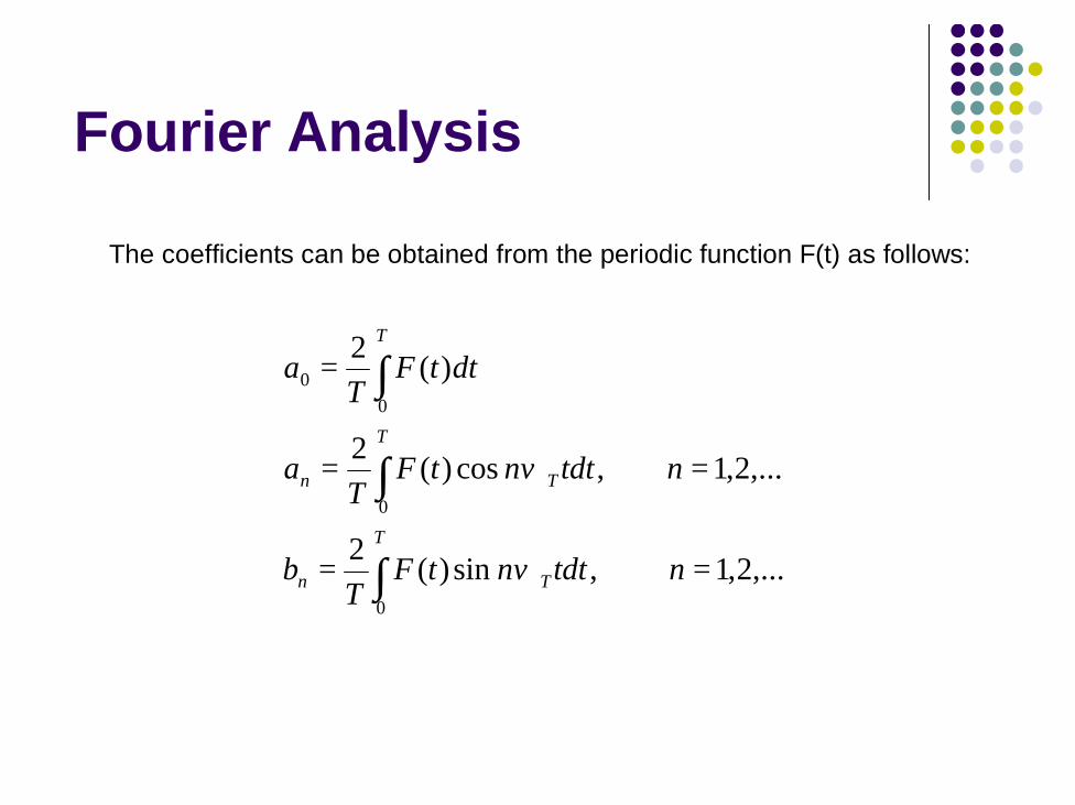
Fourier Analysis

The coefficients can be obtained from the periodic function F(t) as follows:

,...2,1,sin)(2

,...2,1,cos)(2

)(2

0

0

00

==

==

=

∫

∫

∫

ntdtntFT

b

ntdtntFT

a

dttFT

a

T

Tn

T

Tn

T

ϖ

ϖ

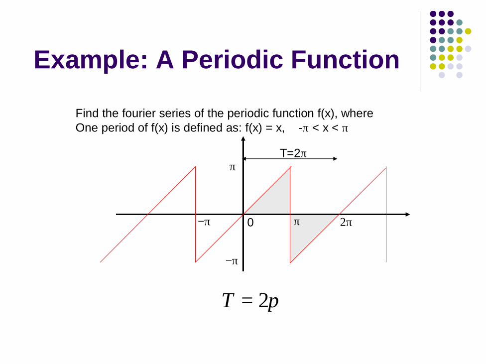
Example: A Periodic Function

Find the fourier series of the periodic function f(x), whereOne period of f(x) is defined as: f(x) = x, -π < x < π

π2=T

T=2π

0 π 2π−π

π

−π

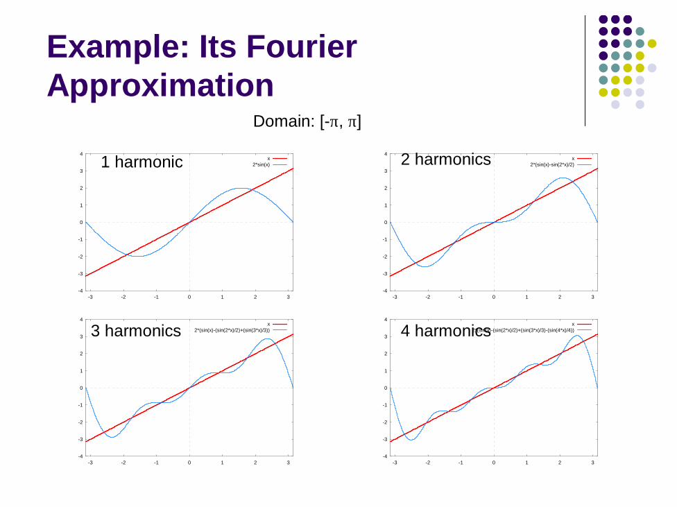
Example: Its Fourier Approximation

-4

-3

-2

-1

0

1

2

3

4

-3 -2 -1 0 1 2 3

x2*sin(x)

-4

-3

-2

-1

0

1

2

3

4

-3 -2 -1 0 1 2 3

x2*(sin(x)-sin(2*x)/2)

-4

-3

-2

-1

0

1

2

3

4

-3 -2 -1 0 1 2 3

x2*(sin(x)-(sin(2*x)/2)+(sin(3*x)/3))

-4

-3

-2

-1

0

1

2

3

4

-3 -2 -1 0 1 2 3

x2*(sin(x)-(sin(2*x)/2)+(sin(3*x)/3)-(sin(4*x)/4))

1 harmonic 2 harmonics

3 harmonics 4 harmonics

Domain: [-π, π]

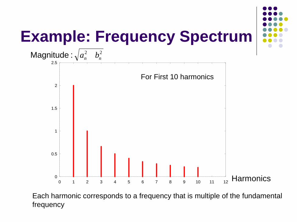
Example: Frequency Spectrum 22nn ba + :Magnitude

Harmonics

For First 10 harmonics

0

0.5

1

1.5

2

2.5

0 1 2 3 4 5 6 7 8 9 10 11 12

Each harmonic corresponds to a frequency that is multiple of the fundamental frequency

Complex Form of Fourier Series

θθθ sincos je j +=

By substituting Euler’s Expresssion into Fouries expansion:

,....2,1,0,1,2...,)(1

)(

2

2

−−==

=

∫

∑

−

−

∞

−∞=

ndtetFT

c

dtectF

T

T

tjnn

tjn

nn

T

T

ω

ω

It can be shown that the following is true:

cn are the complex Fourier coefficients

Digital Modulation - Continuesl Line Coding

l Base-band signals are represented as line codes

UnipolarNRZ

BipolarRZ

ManchesterNRZ

Tb

Tb

Tb

V0

V

-VV

-V

1 0 1 0 1 0 1

Pulse Shaping Techniquesl Effect of bandlimited channel: l Rectangular pulses?l Pulses will spread in timel Each symbol will interfer succeeding symbols (ISI) l Increase the symbol error probability (SER).

l How to mitigate ISI?l increase the channel bandwidth (usually infeasible)l design pulse shapes carefully (desirable & popular)

l Spectral shaping is usually done through baseband or IF processing.

l Objectives of pulse shaping techniques:l Minimize the ISIl Minimize the spectral width of a modulated digital signal

Pulse Shaping Techniques

l Nyquist Criterion for ISI Cancellation l rectangular "brick-wall" filter

l Raised Cosine Rolloff Filterl Gaussian Pulse-shaping Filter

Nyquist Criterion for ISI Cancellationl Nyquist was the first to solve the problem of overcoming ISI while

keeping the transmission bandwidth low. l To nullify the effect of ISI, the overall response of the communication

system (including transmitter, channel, and receiver) should be designed as follows:

l Rectangular "brick-wall" filter (ideal low-pass filter)l Minimize the spectral width (preferable)l Strong side lobes in time domain (sensitive to timing error)

( )sin( ) s

effs

t Th t

t Tπ

π=

1( )effs s

fH ff f

= Π

, 0( )

0, 0eff s

K nh nT

n=

= ≠

Nyquist Criterion for ISI Cancellation

f

( )effH f

Raised Cosine Rolloff Filterl The most popular pulse shaping filter used in

mobile communications. l Transfer function

α is the rolloff factor which ranges between 0 and 1.

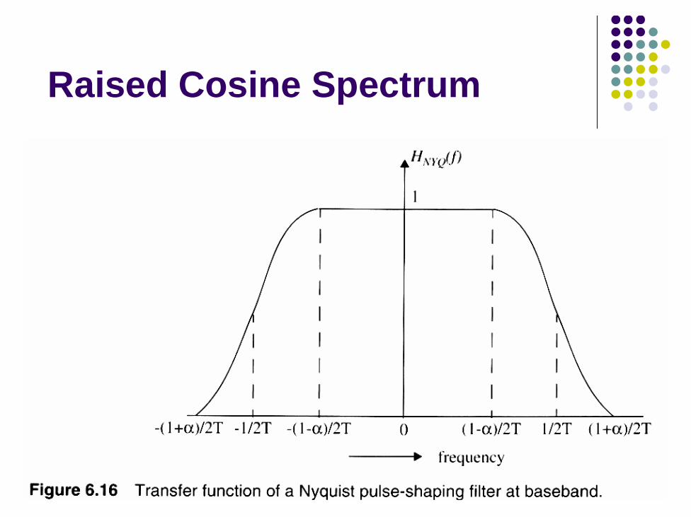
Raised Cosine Spectrum

Raised Cosine Rolloff Filterl Impulse response of the cosine rolloff filter

l A raised cosine filter belongs to the class of filters which satisfy the Nyquist criterion.

l As the rolloff factor α increases, the bandwidth of the filter also increases, and the time sidelobe levels decrease in adjacent symbol slots. This implies that increasing α decreases the sensitivity to timing jitter, but increases the occupied bandwidth.

Raised Cosine pulses

Spectrum of Raised Cosine pulse

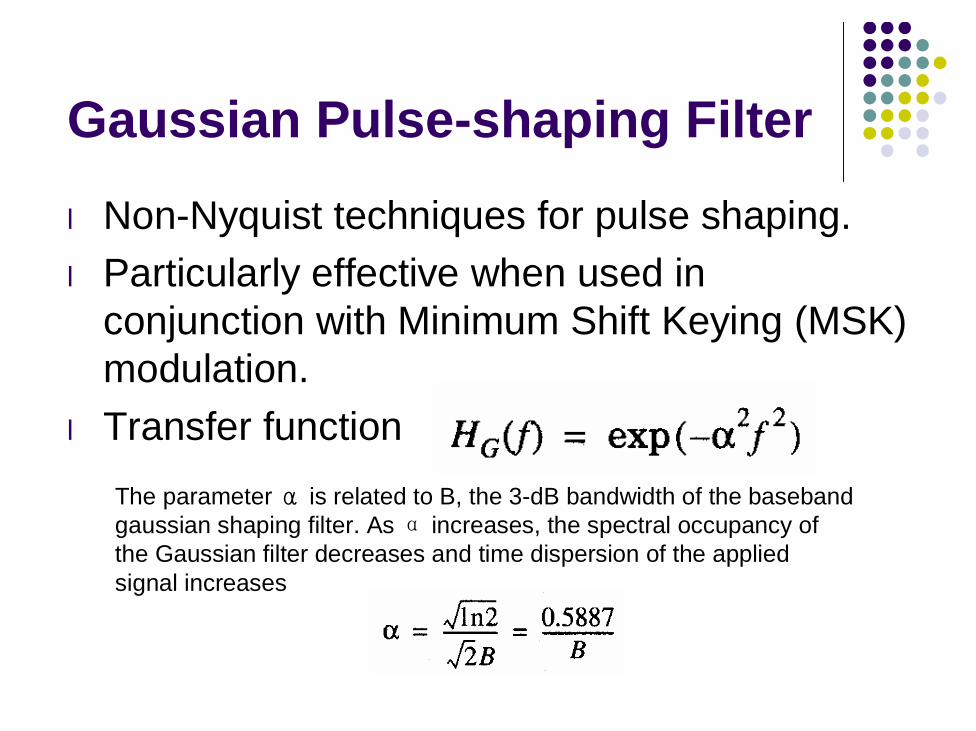
Gaussian Pulse-shaping Filter

l Non-Nyquist techniques for pulse shaping. l Particularly effective when used in

conjunction with Minimum Shift Keying (MSK) modulation.

l Transfer functionThe parameter α is related to B, the 3-dB bandwidth of the baseband gaussian shaping filter. As α increases, the spectral occupancy of the Gaussian filter decreases and time dispersion of the appliedsignal increases

Gaussian Pulse-shaping Filter

l The impulse response of the Gaussian filter

Geometric Representation of Modulation Signal

l Digital Modulation involvesl Choosing a particular signal waveform for transmission for

a particular symbol or signall For M possible signals, the set of all signal waveforms are:

)}(),...,(),({ 21 tststsS M=

l For binary modulation, each bit is mapped to a signal from a set of signal set S that has two signals

l We can view the elements of S as points in vector space

Geometric Representation of Modulation Signall Vector space

l We can represented the elements of S as linear combination of basis signals.

l The number of basis signals are the dimension of the vector space.

l Basis signals are orthogonal to each-other. l Each basis is normalized to have unit energy:

signal. basis the is thi

i

it

dttE

)(

1)(2

φ

φ∫∞

∞−

==

Example

{ })(),(

)2cos(2)(

)2cos(2)(

)2cos(2)(

11

1

2

1

tEtES

tfT

t

tfTEts

tfTEts

bb

cb

cb

b

cb

b

φφ

πφ

π

π

−=

=

≤≤−=

≤≤=

b

b

T t 0

T t 0

bE− bE

Q

I

The basis signal

Two signal waveforms to be used for transmission

Constellation Diagram Dimension = 1

Constellation Diagram

l Properties of Modulation Scheme can be inferred from Constellation Diagraml Bandwidth occupied by the modulation increases as

the dimension of the modulated signal increasesl Bandwidth occupied by the modulation decreases as

the signal_points per dimension increases (getting more dense)

l Probability of bit error is proportional to the distance between the closest points in the constellation. § Bit error decreases as the distance increases (sparse).

Linear Modulation Techniques

l Classify digital modulation techniques as: l Linear§ The amplitude of the transmitted signal varies linearly with

the modulating digital signal, m(t). § They usually do not have constant envelope. § More spectral efficient. § Poor power efficiency§ Examples: QPSK,OQPSK.

l Non-linear

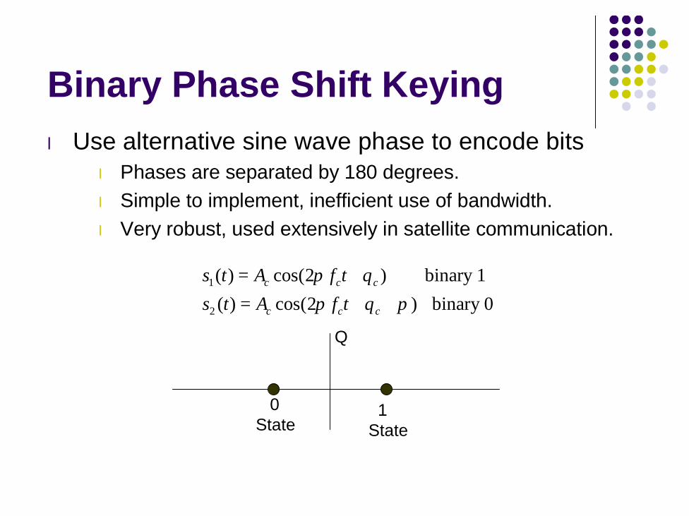
Binary Phase Shift Keyingl Use alternative sine wave phase to encode bits

l Phases are separated by 180 degrees. l Simple to implement, inefficient use of bandwidth. l Very robust, used extensively in satellite communication.

Q

0State

1 State

1

2

( ) cos(2 ) binary 1( ) cos(2 ) binary 0

c c c

c c c

s t A f ts t A f t

π θπ θ π

= += + +

BPSK ExampleData

Carrier

Carrier+ π

BPSK waveform

1 1 0 1 0 1

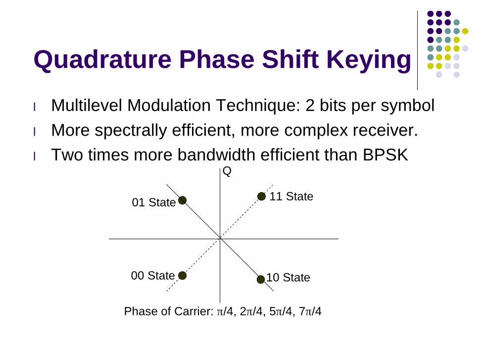
Quadrature Phase Shift Keyingl Multilevel Modulation Technique: 2 bits per symboll More spectrally efficient, more complex receiver. l Two times more bandwidth efficient than BPSK

Q

11 State

00 State 10 State

01 State

Phase of Carrier: π/4, 2π/4, 5π/4, 7π/4

4 different waveforms

-1.5-1

-0.50

0.51

1.5

0 0.2 0.4 0.6 0.8 1 -1.5-1

-0.50

0.51

1.5

0 0.2 0.4 0.6 0.8 1

-1.5-1

-0.50

0.51

1.5

0 0.2 0.4 0.6 0.8 1 -1.5-1

-0.50

0.51

1.5

0 0.2 0.4 0.6 0.8 1

11 01

0010

cos+sin -cos+sin

cos-sin -cos-sin

Constant Envelope Modulation

l Amplitude of the carrier is constant, regardless of the variation in the modulating signall Better immunity to fluctuations due to fading. l Better random noise immunityl Power efficient

l They occupy larger bandwidthl Examples: FSK, MSK, GMSK

Frequency Shift Keying (FSK)l The frequency of the carrier is changed according

to the message state (high (1) or low (0)).

0)(bit Tt0 1)(bit Tt0

b

b

=≤≤∆−==≤≤∆+=

tffAtstffAts

c

c

)22cos()()22cos()(

2

1

ππππ

Continues FSK

))(22cos()(

))(2cos()(

∫∞−

+=

+=t

fc

c

dxxmktfAts

tfAts

ππ

θπ

Integral of m(x) is continues.

1 1 0 1

FSK Example

Data

FSK Signal

Combined Linear and Constant Envelope Modulation Techniquesl Modem modulation techniques exploit the fact that digital

baseband data may be sent by varying both the envelope and phase (or frequency) of an RF carrier.

l M-ary signaling: two or more bits are grouped together to form symbols, where M=2n (n is an integer). l MASKl MPSKl MFSKl MQAM

l M-ary modulation schemes achieve better bandwidth efficiency at the expense of power efficiency.

M-ary Phase Shift Keying (MPSK)

l Modulated signal

l Probability of symbol error in an AWGN channel

( )2( ) cos 2 1 ,0 , 1,2,...,2

si c s

s

E Ms t f t i t T i MT

ππ

= + − ≤ ≤ =

2

0 0

log2 sin 2 sins be

E E MP Q QN M N M

π π ≤ =

8-PSK Signal Constellation

M-ary Quadrature Amplitude Modulation (QAM)

l Modulated signal

l Probability of symbol error in an AWGN channel

( ) ( )min min2 2( ) cos 2 sin 2

,0 , 1, 2,...,

i i c i cs s

s

E Es t a f t b f tT T

t T i M

π π= ⋅ + ⋅

≤ ≤ =

min

0 0

321 14 1 4 1( 1)

ave

EEP Q QN M NM M

≅ − = − −

16-QAM Signal Constellation