Chapter 6Heap and Its Application

We have already discussed two sorting algo-

rithms: Insertion sort and Merge sort; and also

witnessed both Bubble sort and Selection sort

in a project.

Insertion sort takes Θ(

n2)

time in the worst

case, but it is a fast in-place algorithm for small

input sizes. An algorithm is in-place if only a

constant number of elements of the input are

stored outside. Merge sort runs in Θ(n logn),

but it is not an in-place algorithm (?).

We will discuss two more sorting algorithms:

heapsort in this chapter and quicksort in the

next one.

Heapsort runs in Θ(n logn), based on an inter-

esting data structure of heap; while quicksort

has an average-case running time of Θ(n logn)

and a worst-case running time of Θ(

n2)

, but

often outperforms heapsort in practice.

1

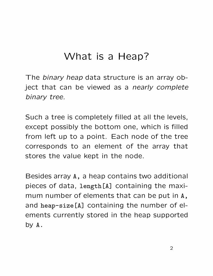
What is a Heap?

The binary heap data structure is an array ob-

ject that can be viewed as a nearly complete

binary tree.

Such a tree is completely filled at all the levels,

except possibly the bottom one, which is filled

from left up to a point. Each node of the tree

corresponds to an element of the array that

stores the value kept in the node.

Besides array A, a heap contains two additional

pieces of data, length[A] containing the maxi-

mum number of elements that can be put in A,

and heap-size[A] containing the number of el-

ements currently stored in the heap supported

by A.

2

Heap vs array

When representing a binary tree with A, the

root of the tree is kept in A[1]. In general,

given the index i of a node in the tree, the

indices of its parent in the tree(Parent(i)), its

left child(Left(i)), and its right child(Right(i)),

can be computed, respectively, as⌊

i2

⌋

,2i, and

2i + 1.

On the other hand, given a binary tree, we

can also map all the nodes in the tree into the

elements of an array A by labeling the root to

A[1], and once a node is mapped to an index

i, its left child, and right child are mapped to

2i and 2i + 1.

Hence, there is a 1-1 correspondence between

a binary tree and an array. Such a relationship

is particularly appropriate for a nearly complete

binary tree (?).

3

Two kinds of heaps

A max-heap satisfies the following additional

property of A[Parent(i)] ≥ A[i], namely, the

value of every node, except the root, is no

more than that of its parent; while a min-heap

satisfies the property of A[Parent(i)] ≤ A[i],

that is, for all the nodes, except the root, its

value is no less than that of its parent.

Hence, the root of a max-heap keeps the largest

value, while the root of a min-heap keeps the

smallest.

We will use the max-heap for the heapsort al-

gorithm; while the min-heap is often used for

the priority queue data structure and schedul-

ing problems, which we will discuss in CS4310.

Homework: Exercises 6.1-6, 6.1-3(*), 6.1-4

and 6.1-5(*).

4

A few notions

When regarding the heap as a tree, we define

the height of a node in a heap to be the num-

ber of edges on the longest simple path from

this node to a leaf, and define the height of a

heap to be the height of its root.

We also define the level of a node in a tree to

be the length of the path from this node to

the root. Thus, the level of the root is just

0, and the maximum level of a tree equals its

height.

In a complete binary tree, every node, except a

leaf, has exactly two children. Thus, the root,

at level 0, has two children, each of them, at

level 1, has two children, thus four nodes at

level 2.

In general, at level i ∈ [0, H], there are exactly

2i nodes. So what?

5

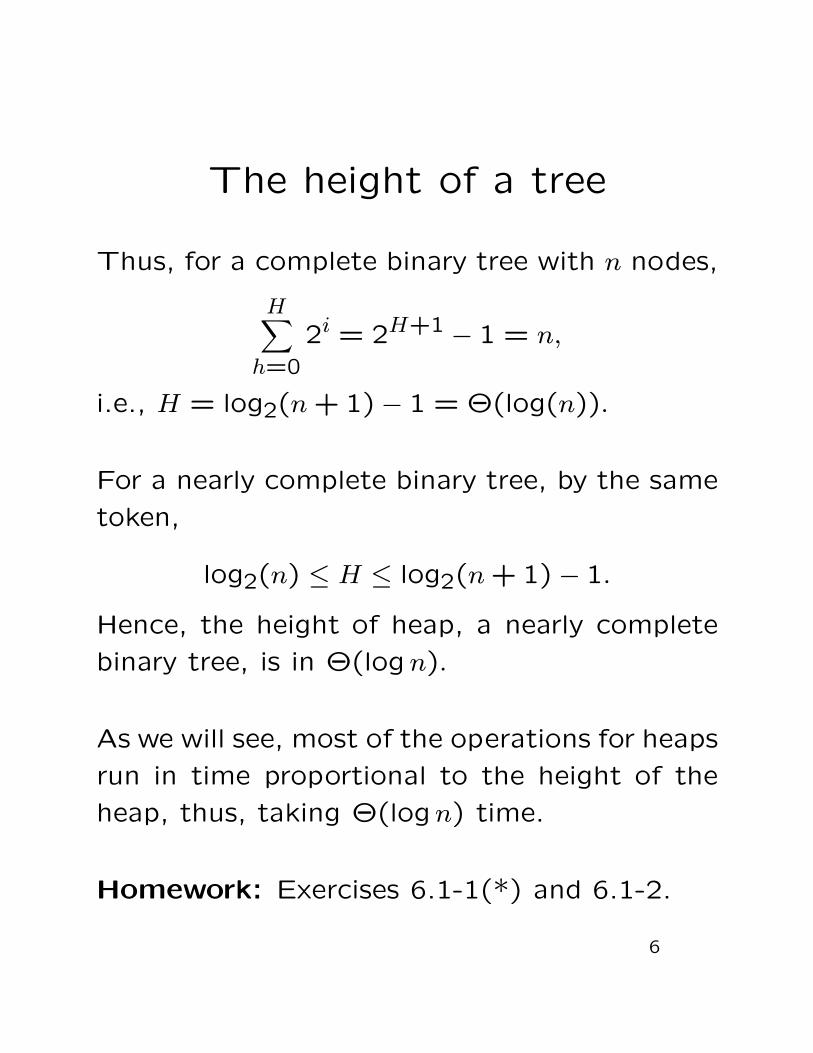
The height of a tree

Thus, for a complete binary tree with n nodes,

H∑

h=0

2i = 2H+1− 1 = n,

i.e., H = log2(n + 1)− 1 = Θ(log(n)).

For a nearly complete binary tree, by the same

token,

log2(n) ≤ H ≤ log2(n + 1) − 1.

Hence, the height of heap, a nearly complete

binary tree, is in Θ(logn).

As we will see, most of the operations for heaps

run in time proportional to the height of the

heap, thus, taking Θ(logn) time.

Homework: Exercises 6.1-1(*) and 6.1-2.

6

Basic heap procedures

We now present the details of several basic

procedures, and show how to apply them in

the heapsort algorithm:

The Max-Heapify procedure maintains the heap

property, running in Θ(logn).

The Build-Max-Heap procedure builds up a max-

heap in Θ(n).

The Heapsort algorithm solves the sorting prob-

lem in Θ(n logn) time.

The Max-Heap-Insert, Heap-Extract-Max,

Heap-Increase-Key, and Heap-Insert procedures,

all running in Θ(logn), allow the max-heap to

be used as a max priority queue.

7

Stay heapy

There are two inputs for the Max-Heapify pro-

cedure, an array A corresponding to a binary

tree, and an index i of a position in A.

When it is called, it is assumed (precondition)

that the binary trees rooted at Left(i) and

Right(i) are both max-heaps, but A[i] may be

smaller than its children, thus A might not be

a max-heap.

The goal of this procedure is to let the value of

A[i] “float down” so that the subtree rooted

at i becomes a max-heap.

8

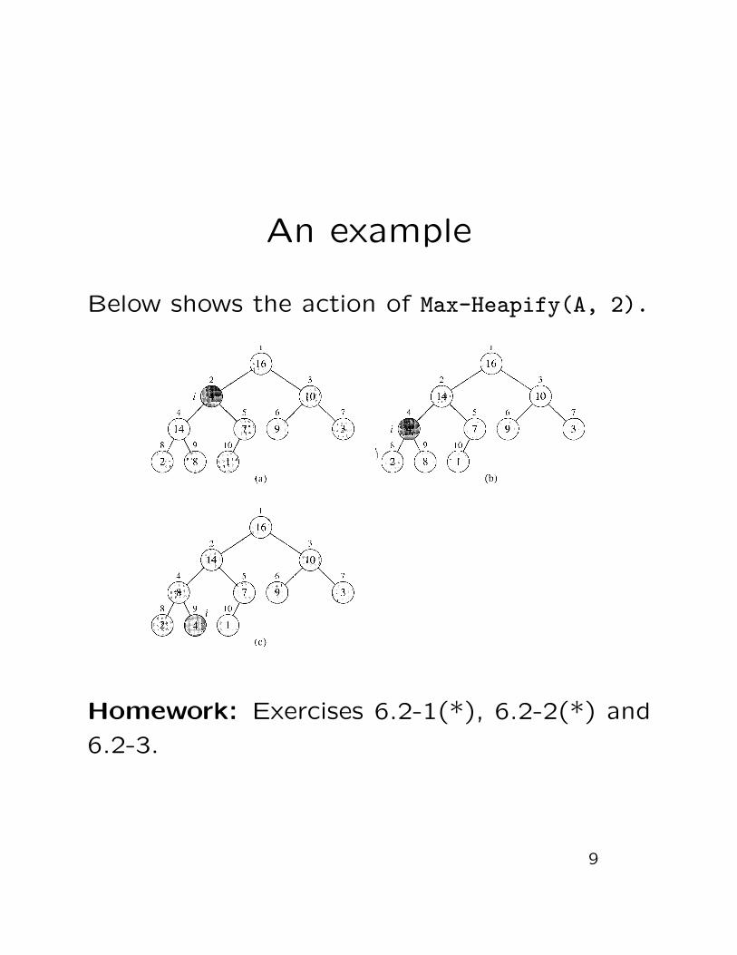
An example

Below shows the action of Max-Heapify(A, 2).

Homework: Exercises 6.2-1(*), 6.2-2(*) and

6.2-3.

9

The code

MAX-HEAPIFY(A, i)

1. l<-Left(i)

2. r<-Right(i)

3. if l<=heap-size[A] and A[l]>A[i]

4. then largest<-l

5. else largest<-i

6. if r<=heap-size[A] and A[r]>A[largest]

7. then largest<-r

8. if largest != i

9. then exchange(A[i], A[largest])

10. MAX-HEAPIFY(A, largest)

At each step, the largest of A[i], A[Left(i)]

and A[Right(i)] are determined in lines 3-7. If

A[i] does not hold the largest one, its value is

exchanged with that of A[i].

Now A[largest] contains the original value of

A[i], which may be smaller than its child, thus

the process repeats itself until it hits the end.

10

The running time

It takes Θ(1) to go through lines 1–7. It then

might run recursively on a subtree rooted at

one of its children.

The worst case happens when the nodes of

the last row of the heap also occur in the cho-

sen subtree, when the chosen subtree has 2n−13

nodes (Cf. Next page). Hence, the recurrence

for the worst case is

T(n) ≤ T

(

2n

3

)

+ Θ(1).

It is then easy(?) to see that

T(n) = O(logn).

Homework: Exercises 6.2-5 and 6.2-6(*).

11

The worst case...

Let T(r, Tl, Tr) stand for a binary tree with r

being its root, Tl (Tr) being its left (right) sub-

tree, and let its height be h. When T is a heap,

a worst case is that the height of Tr is h − 2,

and that of Tl is h−1, and the bottom layer of

Tl is completely filled.

By the results as stated in page 5, the bottom

layer of Tl contains exactly 2h−1 nodes. More-

over, the first h−2 layers of Tl and Tr contains∑h−2

j=0 2j = 2h−1 − 1 nodes.

Thus, T contains 2(2h−1 − 1)+2h−1 plus one

more vertex for r, i.e., n = 3× 2h−1 − 1 nodes,

i.e., 2h−1 = n+13 .

Finally, Tl contains 2h−1 = 2×2h−1−1 nodes,

which is exactly 2n−13 nodes.

12

Build a heap

We already know that the elements in the sub-

array A[⌊

n2

⌋

+ 1, n]

are all leaves. For example,

when n is even, the left (right) child of

A[(⌊

n2

⌋)

+ 1]

is A[n+2] (A[n+3]), which can-

not be in A. What about the case when n is

odd?

Thus, all such elements are necessarily heaps.

The following procedure goes through the re-

maining nodes backwards (Why?) and runs

MAX-HEAPIFY on each and every one of them.

BUILD-MAX-HEAP(A)

1. heap-size[A]<-length[A]

2. for i<-length[A]/2 downto 1

3. do MAX-HEAPIFY(A, i)

It can be shown that it takes Θ(n) to complete

(Page 17-19).

13

An example

Below shows the action of this procedure.

Homework: Exercises 6.3-1 and 6.3-2(*).

14

The correctness

We will show that the following loop invariant

does hold:

At the start of each iteration of the for

loop, each node i+1, i+2, · · · , n is the

root of a max heap.

Indeed, prior to the first iteration, i =⌊

n2

⌋

.

Each of the node⌊

n2

⌋

+ 1,⌊

n2

⌋

+ 2, · · · , n is a

leaf, thus trivially a max-heap.

15

Assume that before a loop, the loop invariant

holds, and the value of the loop variable i is i0.

Since both Left(i0) and Right(i0) are strictly

larger than i0, thus, by the loop invariant, both

the left-subtree and the right-subtree of node

i0 are max-heaps. Hence, the precondition

of executing Max-Heapify (Cf: Page 8) is met,

which makes the tree rooted at i0, into a max-

heap, while preserving the heap properties of

all of the subtrees rooted at j ∈ [i0 + 1, n].

Now, all the trees rooted at [i0, i0 + 1, . . . , n]

are max-heaps.

At the end of this loop, the loop variable i

is decremented by 1 to contain i0 − 1, thus

withholding the invariant.

At the end of the procedure, the loop variable

becomes 0, thus, all the subtrees rooted at

1,2, · · · , n are max-heaps. In particular, the one

rooted at 1 is a max-heap.

16

The running time

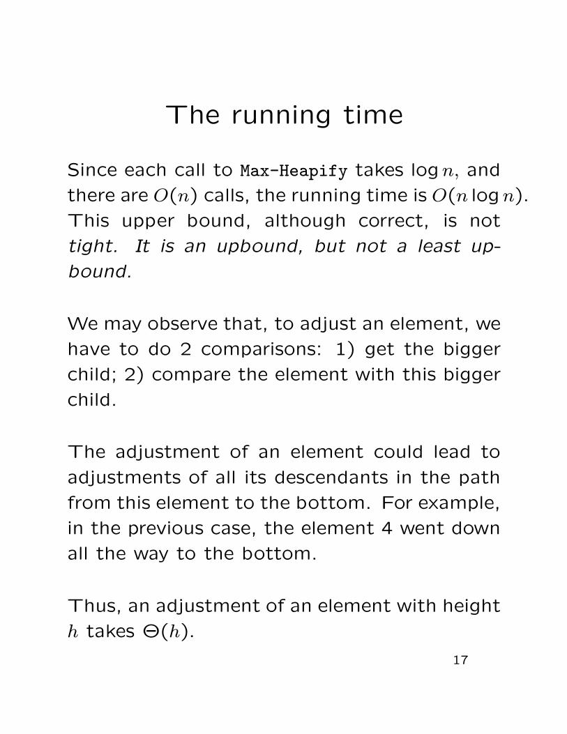
Since each call to Max-Heapify takes logn, and

there are O(n) calls, the running time is O(n logn).

This upper bound, although correct, is not

tight. It is an upbound, but not a least up-

bound.

We may observe that, to adjust an element, we

have to do 2 comparisons: 1) get the bigger

child; 2) compare the element with this bigger

child.

The adjustment of an element could lead to

adjustments of all its descendants in the path

from this element to the bottom. For example,

in the previous case, the element 4 went down

all the way to the bottom.

Thus, an adjustment of an element with height

h takes Θ(h).

17

So what?

To build a heap, we have to adjust all the ele-

ments, if we consider the adjustment of all the

leaves are trivial.

Put in everything, the time complexity of the

initialization process is bounded by the sum of

the heights of all the nodes in the heap.

A complete binary tree is a nearly complete

binary tree where its bottom level is also com-

pletely filled, so such a tree contains at least as

many nodes as a nearly complete binary tree

with the same height.

18

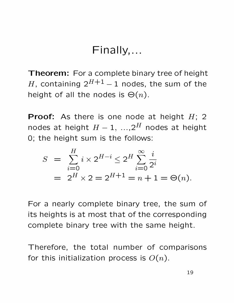
Finally,...

Theorem: For a complete binary tree of height

H, containing 2H+1 − 1 nodes, the sum of the

height of all the nodes is Θ(n).

Proof: As there is one node at height H; 2

nodes at height H − 1, ...,2H nodes at height

0; the height sum is the follows:

S =H∑

i=0

i × 2H−i≤ 2H

∞∑

i=0

i

2i

= 2H × 2 = 2H+1 = n + 1 = Θ(n).

For a nearly complete binary tree, the sum of

its heights is at most that of the corresponding

complete binary tree with the same height.

Therefore, the total number of comparisons

for this initialization process is O(n).

19

We are ready for Heapsort

Given (16,14,10,8,7,9,3,2,4,1), we go through

the following process to sort it:

Isn’t this neat? ,

20

The heapsort algorithm

The heapsort algorithm, when applied to a list

of numbers kept in an array A, starts by build-

ing a max-heap out of A, so that the largest

element ends up at A[1].

The process continues by exchanging this largest

element with A[n]. Since A[n] is in its final

place, we cut it off the heap.

The new A[1] might violate the heap property

for A[1, n-1], thus we call Max-Heapify(A, 1)

to restore A[1, n-1] into a heap.

Now that A[1] again contains the largest ele-

ment of the leftover, the process will repeat

until the shrinking heap contains only one el-

ement, which is the smallest of all, and is al-

ready located in the proper place.

We are done.

21

The code

HEAPSORT(A)

1. BUILD-MAX-HEAP(A)

2. for i<-length[A] downto 2

3. do exchange(A[1], A[i])

4. heap-size[A]<-heap-size[A]-1

5. MAX-HEAPIFY(A,1)

The algorithm runs in O(n logn), since the ini-

tialization takes O(n), and for the n − 1 loop,

MAX-HEAPIFY always runs at O(logn).

Homework: Make a more detailed analysis of

the last statement. (Hint: You need to go

back to Chapter 3.) Exercises 6.4-1, 6.4-2(*)

and 6.4-3(*).

22

Priority queues

A priority queue maintains a set S of elements,

each of which is associated with a key. We

assume there exists a way for us to compare

the keys of all the elements.

Priority queue can be used to schedule jobs

to be processed with limited resource. Jobs

come in with different, adjustable, priority, and

will be inserted into such a queue. When a

resource becomes available, the job with the

maximum priority will be chosen and deleted

from the queue. Priority of a job might be

increased after its joining the queue.

Priority queue is a quite valuable and useful

data structure, and have been made extensive

use in operating systems.

23

What should we do with it?

A max priority queue supports the following

operations:

INSERT(S, x) inserts x into S.

MAXIMUM(S) returns the element of S with the

largest key.

EXTRACT-MAX(S) removes and returns the ele-

ment of S with the largest key.

INCREASE-KEY(S, x, k) increases the value of

element x to the new value k, which is no

smaller than its original key value.

The implementation of these operations de-

pend on the organization of such a queue.

24

Priority queue implementation

We can implement such a priority queue with

an initially empty unsorted array, and use a

position to indicate where another element can

be inserted, initially set at 1.

To insert an item, you just add it in the first

available place in Θ(1) time. To look for the

maximum element in the list, you have to do a

bear/corn style search in O(n), where n is the

number of elements as contained in such a list.

Once you have extracted the maximum ele-

ment from the list, you also have to fill this

“hole” by moving all the elements to the right

of such a maximum element one position to

the left, also in O(n).

Finally, when you want to increase the value

of an element, you can just do it in Θ(1).

25

Other implementations

You can also implement a priority queue with

a sorted array, which also takes linear time for

some of the four operations.

It turns out that the heap structure is an ex-

cellent, Θ(logn), implementation of the pri-

ority queue. More specifically, the heap im-

plementation leads to Θ(1) inspection, and

Θ(logn) running time for insertion, delete-Max

and increase-key operations for a priority queue

containing n elements.

We will mainly discuss the max priority queue,

which always deletes the maximum element.

The min priority queue is the same.

Question: Have you checked the project page

recently?

26

Implementation

When S is implemented with a heap A, the

MAXIMUM(S) operation is simply return A[1].

The code of EXTRACT-MAX takes out the biggest

one, i.e., A[1], fills the “hole” with the last

one, then adjusts the heap.

HEAP-EXTRACT-MAXIMUM(A)

1. if heap-size[A]<1

2. then error "heap underflow"

3. max<-A[1]

4. A[1]<-A[heap-size[A]]

5. heap-size[A]<-heap-size[A]-1

6. MAX-HEAPIFY(A, 1)

7. return max

This procedure runs in O(logn), since it only

does a constant amount of work, besides run-

ning MAX-HEAPIFY once.

27

Key increase

The code increases A[i] to its new value, key,

which might violate the max-heap property /.

Thus, we have to go upwards toward the root

to find a proper place for this newly adjusted

key.

HEAP-INCREASE-KEY(A, i, key)

1. if key < A[i]

2. then error "new key is too small"

3. A[i]<-key

4. while i>1 and A[Parent(i)]<A[i]

5. do exchange(A[Parent(i)], A[i])

6. i<-Parent(i)

This procedure also takes O(logn) since the

length of the path from i to the root is at

most logn, the height of this heap.

28

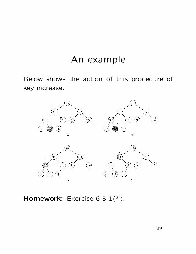
An example

Below shows the action of this procedure of

key increase.

Homework: Exercise 6.5-1(*).

29

Add in another piece

When adding in another element with key, we

naturally expand A, add in an element with the

minimum key value, then call the just discussed

key increase operation to beef up its value to

key.

MAX-HEAP-INSERT(A, key)

1. heap-size[A]<-heap-size[A]+1

2. A[heap-size[A]]<-minInt

3. HEAP-INCREASE-KEY(A, heap-size[A], key)

It is clear that its running time is also O(logn).

Hence, the heap structure can implement a pri-

ority queue in O(logn) time. Yeah! ,

Homework: Exercises 6.5-2, and 6.5-4(*).

30