Sorting signed permutations by inversionsin O(nlogn) time

Krister M. Swenson, Vaibhav Rajan, Yu Lin, and Bernard M.E. Moret

Laboratory for Computational Biology and BioinformaticsEPFL (Ecole Polytechnique Federale de Lausanne), Switzerland

{krister.swenson,vaibhav.rajan,yu.lin,bernard.moret}@epfl.ch

Abstract. The study of genomic inversions (or reversals) has been a mainstay

of computational genomics for nearly 20 years. After the initial breakthrough

of Hannenhalli and Pevzner, who gave the first polynomial-time algorithm for

sorting signed permutations by inversions, improved algorithms have been de-

signed, culminating with an optimal linear-time algorithmfor computing the in-

version distance and a subquadratic algorithm for providing a shortest sequence

of inversions—also known as sorting by inversions. Remaining open was the

question of whether sorting by inversions could be done inO(nlogn) time.

In this paper, we present a qualified answer to this question,by providing two new

sorting algorithms, a simple and fast randomized algorithmand a deterministic

refinement. The deterministic algorithm runs in timeO(nlogn+ kn), wherek

is a data-dependent parameter. We provide the results of extensive experiments

showing that both the average and the standard deviation fork are small constants,

independent of the size of the permutation. We conclude (butdo not prove) that

almost all signed permutations can be sorted by inversions in O(nlogn) time.

1 Introduction

Genomic rearrangements have been the subject of intense research over

the last 10 years. Initially identified in the 1920s in the fly genome through

genetic studies [17, 18], then studied in detail in chloroplast organelles in

the 1980s (for instance in a series of papers from Palmer’s lab, beginning

with [12, 13]), they were brought to the attention of the computational

community in the early 1990s [14]. A large number of papers have since

been published on the combinatorics and algorithmics of genomic rear-

rangements (see [11] for a survey and [7] for a thorough mathematical

treatment). Starting at the beginning of this century, genomic rearrange-

ments have assumed much more importance with the advent of whole-

genome sequencing and the emergence of comparative genomics as a

major discipline in biocomputing.

Of the various genomic rearrangements studied, perhaps thesimplest

and best documented is theinversion(also called reversal in much of the

Computer Science literature), through which a segment of a chromosome

is reversed in place. In 1987, Day and Sankoff [6] formalizeda model of

genomic inversions in which a chromosome is represented as apermuta-

tion of signed gene indices, the sign indicating the direction of transcrip-

tion of the gene; in this framework, an inversion acts on an interval of the

permutation by reversing the order in which the indices appear within the

interval and by flipping the sign of each index. Sankoff laterprovided a

probabilistic model [15] and posed two fundamental questions about in-

versions in this framework: given two signed permutations on the same

index set, what is the smallest number of inversions required to transform

one permutation into the other and what is a sequence of inversions im-

plementing this transformation [14]. The first problem is thus to compute

an edit distance, where the edit operation is the inversion;the second is

to return an edit sequence—a problem usually known as “sorting,” since

a simple re-indexing can turn one of the permutations into the identity.

Many years of work were needed to ascertain the complexity ofeach of

these problems. The breakthrough came in 1995, when Hannenhalli and

Pevzner provided a a polynomial-time algorithm to solve both problems.

(In contrast, in 1997, Caprara [5] showed that both problemswere NP-

hard if phrased in terms of unsigned permutations.) The running time

for both problems has been steadily reduced over the years. In 2001, our

group gave an optimal linear-time algorithm to compute the edit distance

[1]; and in 2004, Tannier and Sagot [20], building on the workof Ka-

plan and Verbin [9], gave aO(n√

nlogn) algorithm to produce a sorting

sequence. Remaining open was the question of whether signedpermuta-

tions can be sorted by inversions inO(nlogn) time, just like sorting plain

numbers.

In this paper, we give a qualified positive answer to this question

by describing two new algorithms for sorting signed permutations by

inversions. The first is a randomized algorithm that runs in guaranteed

O(nlogn) time, but may fail; successive restarts reduce the probability

of failure, but we cannot guarantee that every permutation will be sorted

with high probability with a finite number of restarts, so that it is not a

true Las Vegas algorithm. (Indeed, we give a family of permutations that

cannot be sorted by this algorithm regardless of the number of restarts.)

The other is a deterministic algorithm that always sorts thepermutation

and runs inO(nlogn+ kn) time, wherek is the number of successive

“corrections” (detailed in Section 5) that must be applied—a value, inci-

dentally, that is not related to the edit distanced, although it is bounded

by it. We give a family of permutations for whichk is Θ(n) (the worst-

case value fork) and thus for which our sorting algorithm will run in

quadratic time. However, we present the results of very extensive exper-

imentation showing that the expected value and the standarddeviation

of k are small constants (less than 1), independent ofn, so that the run-

ning time of the algorithm is, with high probability,O(nlogn). Thus we

conclude (but do not prove) that almost all permutations canbe sorted in

optimalO(nlogn) time.

2 Preliminaries

A permutationπ is written as(π1π2 . . .πn), where each elementπi is a

signed integer and the absolute values of these elements areall distinct

and form the set{1,2, . . . ,n}. The absolute value ofπi is denoted by

|πi|. An inversionρ(i, j) on a permutationπ = (π1 . . .πi . . .π j . . .πn) re-

verses all elements betweenπi andπ j while changing their signs giving

(π1 . . .πi−1−π j . . .−πiπ j+1 . . .πn). We assume that every permutation ofn

elements is framed by elements 0 andn+1. In this way we consider each

permutation to be linear, noting that each linear permutation corresponds

to n+1 circular permutations (of lengthn+1), which are equivalent in

terms of the sequences of inversions used to sort them. Thespanof an

inversionρ(i, j) is the closed interval on the natural numbers[i, j] and

two spans[i, j] and[k, l ] overlap if and only if eitheri < k andk < j or

k < i and j < l .

Two adjacent elements,πi andπi+1 for 0≤ i ≤ n+1, form anadja-

cency. An adjacency is anon-breakpointif and only if we haveπi+1−

πi = 1, otherwise it is abreakpoint. An oriented pair, (πi,π j), in a per-

mutation is a pair of integers with opposite signs such thatπi +π j = ±1.

The inversion induced by an oriented pair(πi,π j), called anoriented in-

version, is ρ(i, j −1) for πi +π j = +1, andρ(i +1, j) for πi +π j = −1.

An oriented inversion always creates a non-breakpoint; we say that it

healsthe breakpoint (or breakpoints—there could be two) to whichthe

elements of the oriented pair belonged before the inversion.

A framed common interval(FCI) [2] of a lengthn permutation is

a substring of the permutation, (as1s2 . . .skb) or (−bs1s2 . . .sk−a) (with

s1s2 . . .sk possibly empty) such that

– for eachi, 1≤ i ≤ k, |a| < |si | < |b|,

– for eachl , |a| < l < |b|, there exists aj, 1≤ j ≤ k, with |sj | = l , and

– the FCI is not a union of shorter intervals with the above properties.

The substrings1s2 . . .sk is thus a (possibly empty) signed permutation of

the integers greater thana and less thanb; elementsa andb are called the

frameelements. The framed interval is said to be common in that it also

exists, in its canonical form(

+a+(a+ 1)+(a+ 2) . . .+b), in the identity

permutation. FCIB is nestedinside FCIA if and only if the left and

right frame elements ofA occur, respectively, before and after the frame

elements ofB.

A componentis comprised of the frame elements from an FCI along

with all elements inside the FCI that are not used for a nestedsubin-

terval. A non-trivial componentis a component that is comprised of at

least 4 elements. Abad componentis a component where all elements

have the same sign. Two components can only overlap at the frame ele-

ments [3]. An inversion is said to beunsafeif it creates a bad component,

otherwise it issafe. A permutation ispositiveif it is not the identity per-

mutation and every element is positive. A positive permutation indicates

the existence of at least one bad component. Any permutationcontaining

bad components can be transformed to another permutation that does not

contain any bad component in linear time [1]. Thus, in the algorithms we

describe, we assume that the input permutation does not contain any bad

components.

3 Background: Data Structures for Permutations

To implement an algorithm for sorting by inversions, we needa data

structure for handling permutations that supports two basic operations:

(i) choose an oriented inversion, and (ii) perform an inversion.

We now describe the data structure of Kaplan and Verbin [9] that

stores a permutation in linear space and allows us to performan inversion

in logarithmic time. The structure is a splay tree, in which the nodes

are ordered by the indices of the permutation, with one additional flag

maintained at each node.

To perform an inversionρ(i, j) between (and including) indicesi and

j, index i − 1 is splayed and the right subtree of the root is split from

the root yielding subtreesT<i andT≥i whereT<i (T≥i) contains all ele-

ments with indices less than (greater than or equal to)i. Next, index j

is splayed inT≥i and again the right subtree is split from its root yield-

ing subtreesTrev andT> j whereT> j contains all elements with indices

greater thanj andTrev contains the elements of the permutation that have

to be reversed. Finally, there are three subtrees:T<i, Trev andT> j . Now,

actually reversing the elements inTrev can takeΘ(n) time sinceΘ(n) el-

ements could be reversed in a single inversion. To achieve logarithmic

time complexity a lazy approach is taken: areversedflag is maintained

in each node, which if turned on indicates that the subtree rooted at the

node is reversed. Now instead of immediately reversing a subtree, we

just set its reversed flag. During an inversion the reversed flag of the root

of Trev is flipped andT<i is joined toTrev to getT≤ j . This is achieved

by makingTrev the right child of the root ofT<i , which still contains the

element at indexi − 1, yielding the treeT≤ j . T≤ j is then joined toT> j

by splaying j in T≤ j , after whichT> j is made the right child of the root

of T≤ j , yielding the final tree which represents the permutation after the

inversion. Since the only operation that takes more than constant time is

the splay and since splaying takes amortized logarithmic time [16], each

inversion takes amortized logarithmic time.

A tree could have several reversed flags, but the invariant maintained

is that an inorder traversal modified by the reversed flags yields the per-

mutation. So to read the permutation one would traverse a reversed sub-

tree in reverse order while flipping signs of elements read. Nested re-

versed flags cancel in the sense that a reversed flag on a node within a

reversed subtree, implies that the inner subtree (rooted atthat node) is

not reversed. Thus, a subtree rooted at a node is reversed if and only if

there is an odd number of reversed flags in the path from the root to the

node (including the node).

When a sequence of inversions is performed, reversed flags can get

nested to arbitrarily deep levels. We can push the flag down a traversed

path in the tree, by flipping the sign of the element in the node, exchang-

ing the left and right subtrees, and flipping the reversed flags in both

children. The reversed flag of a leaf is cleared by just flipping its sign.

Pushing down a flag takes constant time per node so the logarithmic time

complexity of splaying is maintained. By pushing down the flags in the

splay path we ensure that the three subtrees created (T<i , Trev andT> j )

reflect the changes made in all the previous inversions.

This is exactly the data structure described in [9]; it can handle a se-

quence ofd inversions inO(d logn) time. The data structure maintains

only the state of the permutation at each step (in a lazy way).However it

does not maintain information about oriented pairs, nor could it do so ef-

ficiently, as a single inversion could change the orientation of Θ(n) pairs.

Indeed, using this data structure to maintain the information necessary

to choose an oriented inversion at each step would increase the running

time by a factor ofn.

To overcome this problem both Kaplan and Verbin [9] and Tannieret

al. [19] used a two-level version of the data structure in which apermu-

tation is stored in linear blocks of sizeO(√

nlogn) each. Corresponding

to each block is a splay tree that maintains information about all ori-

ented pairs(πi,π j) such that eitherπi or π j is in the block. Performing

an inversion while maintaining information about all oriented pairs takes

O(√

nlogn) time and choosing an inversion at each sorting step takes

O(logn) time, so that the total time complexity of their algorithms is

O(n√

nlogn).

In order to run inO(nlogn) time, these algorithms need to be able

to choose an oriented inversion in logarithmic time and thusinformation

to identify such inversions must also be maintained in logarithmic time

through an inversion.

4 Our Algorithm

Instead of addressing the data structure (by designing a newdata struc-

ture that can somehow processO(n) new pair orientations in logarithmic

time), we address the root question of identifying an oriented inversion.

Our key contribution is that we need not maintain information aboutall

oriented inversions for every permutation at each sorting step—a few

suffice in most cases.

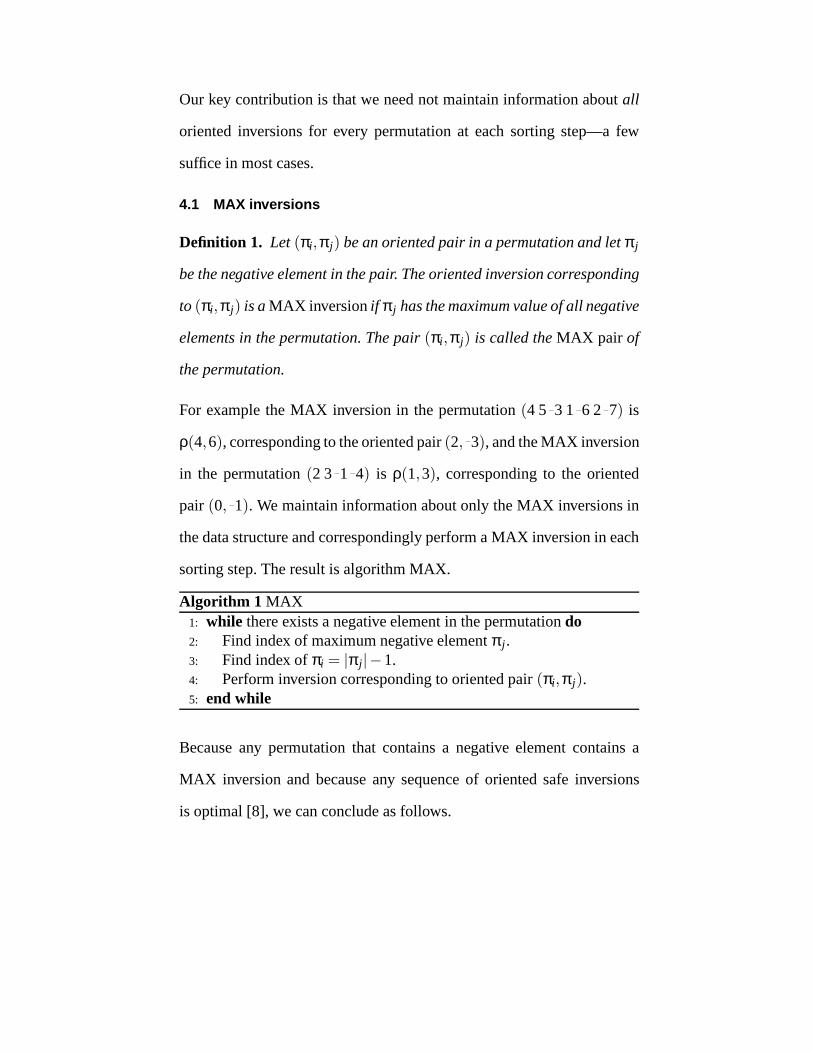
4.1 MAX inversions

Definition 1. Let (πi,π j) be an oriented pair in a permutation and letπ j

be the negative element in the pair. The oriented inversion corresponding

to (πi,π j) is aMAX inversionif π j has the maximum value of all negative

elements in the permutation. The pair(πi ,π j) is called theMAX pair of

the permutation.

For example the MAX inversion in the permutation(4 5−3 1−6 2−7) is

ρ(4,6), corresponding to the oriented pair(2,−3), and the MAX inversion

in the permutation(2 3−1−4) is ρ(1,3), corresponding to the oriented

pair (0,−1). We maintain information about only the MAX inversions in

the data structure and correspondingly perform a MAX inversion in each

sorting step. The result is algorithm MAX.

Algorithm 1 MAX1: while there exists a negative element in the permutationdo2: Find index of maximum negative elementπ j .3: Find index ofπi = |π j |−1.4: Perform inversion corresponding to oriented pair(πi,π j).5: end while

Because any permutation that contains a negative element contains a

MAX inversion and because any sequence of oriented safe inversions

is optimal [8], we can conclude as follows.

Lemma 1. In the absence of unsafe MAX inversions at any sorting step,

algorithm MAX produces an optimal sorting sequence.

Algorithm MAX fails to sort only when it is “stuck” at an all-positive

permutation that is not the identity, which happens when a MAX inver-

sion was unsafe. (We deal with unsafe inversions in the next section.)

The same arguments holdmutatis mutandisif we choose an oriented pair

with the minimum negative element, yielding another algorithm, algo-

rithm MIN. Combining the two strategies and picking one at random at

each step gives us a randomized algorithm: algorithm RAND.

Algorithm 2 RANDwhile there exists a negative element in the permutationdo

randomly select either MAX or MINif MAX then

Find index of maximum negative elementπ j .Find index ofπi = |π j |−1.Perform inversion corresponding to oriented pair(πi,π j).

else ifMIN thenFind index of minimum negative elementπk.Find index ofπl = |πk|+1.Perform inversion corresponding to oriented pair(πk,πl).

end ifend while

4.2 Maintaining information through an inversion

We now show how to maintain information about the maximum nega-

tive element of a permutation through an inversion using thesplay tree

data structure. We describe the process for MAX, but the obvious analog

works for MIN.

Let the maximum negative element of a subtree,MAXneg, be the el-

ement in the subtree that has the maximum value among all negative

elements in the subtree. The minimum positive element,MINpos, of a

subtree is defined similarly. These values are stored in eachnode of the

splay tree. Note that theMAXneg of the root node is the maximum nega-

tive element of the permutation, that is, the negative element of the MAX

pair of the permutation. TheMAXneg of a node is the maximum of the

following three: theMAXneg of the left subtree, theMAXneg of the right

subtree, and the element in the node if the element is negative. Also no-

tice that whenever the reversed flag of a node is turned on,MAXneg and

MINposare swapped. Therefore pushing down a reversed flag applies this

swap to the children, unless there is a cancellation of flags.

A splay operation performs a series of rotations based on thestructure

of the tree and the index being queried. Each rotation changes at most

three edges of a connected subtree while maintaining the binary search

tree property.MAXneg can be recalculated for only the subtree that is

affected, Recall that to perform an inversionρ(i, j) the splay tree is split

into three subtrees which are rejoined after the reversed flag has been set

for one of the trees. The value ofMAXneg can be kept for each of the

subtrees in the process by simply checking the children of the root after

each operation.

By maintaining theMAXneg values in this fashion, one can maintain

the invariant that theMAXneg of the root node is the maximum negative

element of the permutation through any sequence of inversions. Since

calculatingMAXneg takesO(1) time per node, these modifications do not

alter the time complexity of the data structure.

Lemma 2. For any (signed) permutation of size n, there exists a data

structure that handles an inversion in O(logn) time while maintaining

information about the maximum negative element of the permutation.

4.3 Finding the MAX pair

We now describe how to obtain the elements of the MAX pair in a per-

mutation using the modified data structure described above.

First the maximum negative element of the permutation is located. If

the element in a node is not equal to theMAXnegof the node thenMAXneg

of the node lies in either the left subtree or the right subtree of the node.

Therefore starting at the root one can go down the tree looking for the

maximum negative element. Reversed flags must be pushed downalong

the path to ensure thatMAXnegvalues are updated and the correct path is

followed.

To find the second element of the MAX pair, a lookup vector of point-

ers (ofn elements) maps each element to the node that contains the el-

ement. These pointers do not change throughout the computation and

enable constant-time lookup of the node containing the second element

of the MAX pair.

4.4 Finding the indices of the MAX inversion

In absence of reversed flags, the indices of the MAX inversioncan be

obtained directly from the current location of the nodes corresponding to

the MAX pair. However, the presence of a reversed flag indicates nodes

that have outdated indices, forcing additional work to retrieve the correct

indices.

The index of a node (with respect to the current state of the permu-

tation) can be calculated using the index of the parent node and the sizes

of the left and right subtrees. Thus the current index of a node can be

calculated whenever the reversed flag is pushed down from it.The size

of the subtree rooted at a node is easily maintained. If the node is a right

child, then its index is one more than the sum of its parent’s index and the

size of the left subtree. If the node is a left child, then its index is one less

than the difference of its parent’s index and the size of the right subtree.

The index of the root is just the size of its left subtree. Thusstarting at

the root, as the reversed flags are pushed down along any path in the tree,

the current indices can be calculated.

As one traverses the tree from the root searching for the maximum

negative element, the indices are recalculated. After the node correspond-

ing to the second element in the MAX pair is found using the lookup

vector, its updated index can be retrieved by traversing up to the root (us-

ing parent pointers) and returning down the same path, pushing down the

reversed flags and recalculating indices at each node.

4.5 Putting it all together

The previous subsections detail all the steps for performing a MAX in-

version. The time complexity of each of these steps is easy toanalyze.

Pushing down the reversed flag takesO(1) time per node. Thus, find-

ing the maximum negative element and its updated index takesO(logn)

time. Finding the other element of the MAX pair takesO(1) time and ob-

taining its updated index takesO(logn) time. Therefore the complexity

of finding the two indices (steps 2 and 3 in algorithm MAX) isO(logn).

For each inversion, maintainingMAXneg, MINpos, MINneg, andMAXpos

in the nodes takesO(1) time during split and join operations, andO(1)

time for each rotation in the two splays. Therefore performing the inver-

sion in step 4 of algorithm MAX takesO(logn) time. So we have proved:

Theorem 1. For any signed permutation of size n, a data structure exists

that

– allows checking whether there exists an oriented inversionin O(1)

time,

– allows performing a MAX (or MIN) inversion, while maintaining the

permutation, in O(logn) time,

– and is of size O(n).

Theorem 2. In the absence of unsafe inversions at any sorting step, al-

gorithm MAX produces an optimal sorting sequence in O(nlogn) time.

5 Bypassing Bad Components

We saw that algorithms MAX and RAND can get stuck at a positive

permutation by choosing an unsafe inversion. We offer two strategies for

recovery.

5.1 Randomized restarts

For algorithm RAND we can simply restart the computation hoping that

a better outcome is met in the next run. Indeed, the experiments from

Section 6 show that, for most permutations, this simple approach suf-

fices. However, this approach cannot always sort a permutation as there

exists a family of permutations that it cannot handle. For instance, take

the permutation (3 1−4−2): both MAX and MIN inversions are unsafe

because they yield the same positive permutation (3 1 2 4); this small ex-

ample can be extended to any length by appending the requisite number

of positive elements.

5.2 Recovering from an unsafe inversion: Tannier and Sagot’ s ap-

proach

Tannier and Sagot [20] introduced a powerful approach for finding un-

safe inversions and augmenting the sorting sequence till itis optimal.

They noticed that it is computationally difficult to detect an unsafe inver-

sion as it is applied; but it is of course trivial to find out that the process

is stuck at a positive permutation. Their approach is thuspostmortem:

their algorithm traces the sorting process back to the most recent unsafe

inversion and inserts two or more sorting inversions beforethe unsafe

one without invalidating other sorting inversions. (This ensures that the

sorting sequence grows in every trace-back phase.) After the trace-back,

the sorting process continues from the state of the permutation just be-

fore the unsafe inversion. The new inversions that are inserted are chosen

such that the bad component created by the previous unsafe inversion is

no longer created and so, the (previously) unsafe inversionand all the

inversions that followed it can be applied again.

They use anoverlap graphto keep track of the remaining breakpoints

(and whether or not they are oriented). Using the overlap graph they can

find the most recent unsafe inversion, find and insert more inversions be-

fore the unsafe one, and continue sorting without invalidating the inver-

sions that have been applied after the most recent unsafe inversion [20].

However, the process may have to be repeated, as, even after augmenting

the sorting sequence, their algorithm may again get stuck ata positive

permutation.

5.3 Recovering from an unsafe inversion: Our approach

We use the same general idea, but do not maintain the full overlap graph,

as it is too expensive to maintain. Denote byp1 the first positive permu-

tation at which the algorithm gets stuck and bypi the ith such positive

permutation. Recovering from a positive permutationpi involves three

steps: finding the most recent unsafe inversionµi , finding and inserting

two other oriented inversions with the required propertiesthat can be ap-

plied beforeµi , and appending inversions without invalidating those sort-

ing inversions that had been applied after (and including)µi. We describe

each of these steps in turn.

Finding the most recent unsafe inversion: In the trace-back phase,

we undo the inversions that have been done so far in order to find the

most recent unsafe inversionµi . Note that an unsafe inversion is an inver-

sion that, when undone, creates a good component from bad components.

Denote byπ ·Sandπ ·ρ the result of applying the inversions from the se-

quence of inversionsS and the single inversionρ to the permutationπ,

respectively. LetU(π) be the set of unsafe inversions on a permutationπ

and letB(π) be the set of bad components inπ ·µ for µ∈U(π). Undoing

the inversionρ in π ·ρ refers to performingρ onπ ·ρ which yieldsπ, and

undoing the inversionsS= ρ1,ρ2, . . . ,ρn in π ·Srefers to performing the

inversions ofS in the reverse order which yieldsπ ·S·ρn . . .ρ2 ·ρ1 = π.

The sequence of inversions on input permutationπ0 that results in the

positive permutationpi is denoted bySi , sopi = π0 ·Si.

Remark 1.When undoing inversions fromSi, the most recent unsafe in-

versionµi is the first inversion met that turns an element inB(pi) from

bad to good.

Findingµi is not trivial because framed intervals can be nested. For ex-

ample the positive permutation (2 3 6 7 4 5 8 9 10 1) has two compo-

nents: the one framed by the implicit frame elements 0 and 11,and the

nested component framed by the elements 3 and 8. Undoing the inver-

sionρ(2,7) will leave both bad components intact despite the fact that it

occurs within the frame elements of the larger component. Thus, in the

trace-back phase,ρ(2,7) cannot be an unsafe inversion. However, undo-

ing the inversionsµ(5,7) andµ(4,5) will make the inner component good

and so these two inversions, had they been performed, would have been

unsafe. The following remark characterizes undoing an unsafe inversion

in terms of the components inB(pi).

Remark 2.An inversion is the most recent unsafe inversionµi if and

only if it is the most recent inversion to change the indices of a proper

nonempty subset of the elements from some component inB(pi).

The trace-back algorithm is thus as follows: start undoing the inversion

sequenceSi , checking after each inversion whether there exist compo-

nents inB(pi) with both changed and unchanged indices and stop undo-

ing when an unsafe inversion is found. This can be done by keeping an

ancillary splay tree where nodes represent adjacencies in the permutation

rather than permutation elements.

If every adjacency inpi were a breakpoint, the most recent inversion

would be unsafe; the heart of the problem, then, is with non-breakpoints

and how they interact with the undoing of unsafe inversions.We present

a labeling of the ancillary tree so that the safety check can be carried

out by a constant-time comparison on the two adjacencies broken by an

inversion. Each adjacency has a label indicating the innermost overlying

component along with a label that is set only for non-breakpoints. For

a given component, each group of consecutive non-breakpoints (ignor-

ing nested components) gets a unique second label. Thus an inversion

displaces only a fraction of the elements of a component if and only if

both broken adjacencies are labeled as non-breakpoints with the same

component and non-breakpoint labels.

In the example, the permutation (2 3 6 7 4 5 8 9 10 1) has component

label X for adjacencies (0,2), (2,3), (8,9), (9,10), (10,1), and (1,11), and

component label Y for the others. The non-breakpoint labelsare the same

for (2,3), (8,9), and (9,10), but different between (6,7) and (4,5). Inver-

sionρ(2,7) acts upon non-breakpoints with the same pair of labels while

inversionµ(5,7) acts upon non-breakpoints with different component la-

bels andµ(4,5) acts upon non-breakpoints with different non-breakpoint

labels.

We can list the endpoints of the components of a permutation in linear

time [1, 2]. A simple traversal of the permutation, keeping one stack for

each label, can perform the node labeling described above. Thus the setup

of the ancillary tree can be done inO(n) time. LetS1i be the sequence of

inversions applied beforeµi in Si andS2i be the sequence of inversions

applied afterS1i (including µi) in Si . Each safe inversion inS2

i that is

undone will costO(logn) time so the total cost for finding a most recent

unsafe inversion isO(n+ |S2i | logn).

Inserting oriented inversions before the unsafe inversion: Theorem

3 in [19] shows that there always exists two oriented inversionsν1i and

ν2i that are valid on the permutation after the unsafe inversionµi is un-

done in the trace-back phase. According to [19], if inversionsν1i andν2i

have the following properties then all the inversions afterand including

µi are safe, valid, and can be applied at the end of the sorting sequence

on theith iteration:

– the span ofν1i overlaps the span ofµi , and

– either the span ofν2i overlaps the span ofν1i and does not overlap

the span ofµi, or the span ofν2i overlaps the span ofµi and does not

overlap the span ofν1i .

In the following we show how to findν1i andν2i in time proportional

to the size of the bad component that we created.

Lemma 3. Given an unsafe oriented inversion µi and the bad component

b of size m created by µi, one can always find two inversionsν1i andν2i

in O(m) time such that

1. (existence)ν1i andν2i are valid sorting inversions when applied after

S1i .

2. (safety)after applyingν1i andν2i , inversion µi does not create b.

3. (validity) after applyingν1i and ν2i, inversion µi and all the inver-

sions in S2i remain valid sorting inversions and can be applied at the

end of the sorting sequence of the ith run.

Proof. A bad component could have been created in one of three ways

whenµi was applied. Without loss of generality we ignore the symmetric

counterpart to the first case below (both cannot happen at once). We also

ignore the inverted versions of each case where the hurdle created has

only negative elements. This leaves us with three cases to consider.

– (±π0 . . .+l+x1 . . .+xs ±πx . . .−r−xk−1 . . .−xs+1︸ ︷︷ ︸

±πx+1 . . .±πn)

where the braced inversion creates the bad component

b = +l+x1 . . .+xs+xs+1 . . .+xk−1+r.

– (±π0 . . .+l+x1 . . .+xl −xr−1 . . .−xl+1︸ ︷︷ ︸

+xr . . .xk−1+r . . .±πn)

where the braced inversion creates the bad component

b = +l+x1 . . .+xl +xl+1 . . .+xr−1+xr . . .+xk−1+r.

– The third case is the same as the first, except that one or more bad

components are created which span the component+l+x1 . . .+xs+xs+1 . . .+xk−1+r.

For the first case, writeL = +l+x1 . . .+xs and R = −r−xk−1 . . .−xs+1 and

examine the substringsL andR. Since the component(l , . . . , r) is a bad

component, there must exist an elementt in L such that eithert +1 ort−1

is negative and not inL. Assumew is the first such element we encounter

by scanning from+l to +xs. We locate the rightmost−(w−1) or −(w+1)

in R by scanning from−xs+1 to −r. Now, there are two possibilities.

1. The rightmost element is−(w−1). We havew> l +1 and thus(w,−(w−

1)) is an oriented pair; consequently, there exists an orientedinver-

sion, ν1i, which is different fromµi . Now consider the position of

those elements with absolute values between (and including) l and

w−1. Lety be the element with the smallest value that does not ap-

pear to the left ofw in L (such an element must exist becausel is to

the left ofw butw−1 is inR). Thusy−1 must appear to the left ofw

in L. Not thaty cannot be inR, as this would contradict the fact that

w is the leftmost element inL with −(w+1) or −(w−1) in R. Thusy

must be inL and to the right ofw. After applyingν1i , we will have

the oriented pair(y−1,−y), and consequently, another oriented inver-

sion ν2i . Notice that the span ofν1i overlaps the span ofµi and the

span ofν2i overlaps the span ofν1i but not that ofµi . So, the required

properties of safety and validity follow from Theorem 3 in [19].

2. The rightmost element is−(w+1). Note that(w,−(w+1)) is an ori-

ented pair, so that there exists an oriented inversionν11. This inver-

sion must be different fromµi as otherwiseL would a bad component

in itself. Now we examine the substring to the right ofw in L. Letzbe

the element with the largest absolute value in that substring. Consider

the following two cases:

(a) The absolute value ofz is less thanw: we consider the elements

with absolute values in the interval[l ,z]. Lety be the element with

the largest absolute value in[l ,z] that appears to the left ofw (such

an element must exist becausel is to the left ofw but z is to the

right of w in L). y+1 cannot be inR, as this would contradict the

fact thatw is the leftmost element inL with −(w+1) or −(w−1)

in R. Thusy+1 must be inL and to the right ofw. After applying

ν1i , we will have the oriented pair(y,−(y+1)), and consequently,

another oriented inversionν2i . Notice that the span ofν1i overlaps

the span ofµi and the span ofν2i overlaps the span ofν1i but not

that ofµi . So, the required properties of safety and validity follow

from Theorem 3 in [19].

(b) The absolute value ofz is larger thanw+1: We consider the ele-

ments with absolute values in[z, r]. Let y be the element with the

largest absolute value in[z, r] that appears to the left of−(w+1) in

R (such an element must exist becauser is to the left of−(w+1)

in R but z is in L). y− 1 cannot be to the left ofw in L, as this

would contradict the fact thatw is the leftmost element inL with

−(w+1) or −(w−1) in R. Thusy−1 must be either to the right of

w in L or to the right of−(w+1) in R. If y−1 is to the right ofw

in L, the oriented pair(−(y−1),y) defines the oriented inversion

ν2i . Notice that the spans ofν1i andν2i overlap the span ofµi but

ν1i andν2i do not overlap. Ify−1 is to the right of−(w+ 1) in

R, after applyingν1i , we will have the oriented pair(y,−(y−1)),

and consequently, another oriented inversionν2i . In this case the

span ofν1i overlaps the span ofµi and the span ofν2i overlaps the

span ofν1i but not that ofµi. So, the required properties of safety

and validity follow from Theorem 3 in [19].

For the second case (where the span of the unsafe inversion isa proper

subset of the span of the bad component), writeL = +l+x1 . . .+xl , M =

−xr−1 . . .−xl+1 andR= −r−xk−1 . . .−xs+1. In substringsL andR, there must

exist one elementt such that−(t + 1) or −(t −1) is in M and the inver-

sion induced by this pair is notµi . Thus, the oriented pair(t,−(t − 1))

or (t,−(t + 1)) defines the oriented inversionν1i. Sinceν1i is different

from µi , there will be some negative elements after applyingν1i ; assume

that the maximum negative element among them is−y. Thus,y−1 must

be positive and the oriented pair(−y,+(y−1)) defines the other oriented

inversionν2i. It is easy to verify that these inversions have the required

properties.

The linear-time complexity can be achieved by using a lookupvector

that maps each element to its index in the permutation. (Thisis created

in the beginning and maintained throughout the sorting process.) Thus,

for the first case, with a single scan ofL, we can findw and−(w−1) and

with another scan of elements betweenl andw−1 in the lookup vector,

the pair((y−1),−y). The other cases can be analysed similarly. Note that

in no case do we need to scan any element that is not a part ofb. Thus

the inversionsν1i andν2i can be found inO(m) time.

Appending inversions to the sorting sequence: After we get the per-

mutationqi = π ·S1i , we apply the two inversionsν1i andν2i on qi . Now

we would like to ensure that the sequence of inversionsS′i we append

afterν2i does not invalidate the sequenceµi ·S2i . We achieve this by re-

naming the permutationqi in the following way.

By definition, qi · µi has at least one bad component created byµi

along with a possibly nonempty setG(qi ·µi) of good components. The

inversions that sort the components ofG(qi · µi) correspond exactly to

the sequenceS2i . Thus, our desired sequenceS′i of inversions should only

displace (if at all) such components without affecting their structure.

Say there is a componentc of lengthm with left frame elementl .

Thecanonical formc of c is a permutation of lengthm with c[i] = c[i]−

l +1, 1≤ i ≤ m, wherep[i] denotes theith element of a permutationp.

Componentsc andd are said to bestructurally equivalentif and only if

we have ˆc = d.

Lemma 4. Let qi be a permutation without a bad component and µi be

an inversion such that qi ·µi has at least one bad component and a set of

good components G(qi ·µi). There exists a q′i where any sequence S′i that

sorts q′i to the identity, when applied to qi, will result in a permutation

whose only components are those in G(qi ·µi).

Proof. Rename the permutationqi · µi such that all breakpoints from

components inG(qi ·µi) become non-breakpoints and then undoµi to get

q′i . Note that this renaming leaves one structurally equivalent bad compo-

nent in place of each bad component, so that the renaming is unique. A

inversion sequence that sortsq′i to the identity heals all breakpoints from

the bad components inqi ·µi ; moreover, it does not heal any breakpoint

from components ofqi that are inG(qi ·µi) due to the nesting property of

FCIs.

For example, takeqi = (2 3 6 7 4−8 −5 −9 10 −1) andµi = µ(6,7). Now

qi ·µi is (2 3 6 7 4 5 8−9 10 −1), so thatG(qi ·µi) is comprised of the

components framed by the pair (of frame elements) (0,11) andthe pair

(8,10).qi ·µi is renamed toq′i ·µi = (1 2 5 6 3 4 7 8 9 10), yieldingq′i = (1

2 5 6 3−7 −4 8 9 10). The sorting sequenceS′i = (ρ(3,6),ρ(3,4),ρ(4,7))

for q′i can be applied toqi to get (2 3 4 5 6 7 8−9 10−1).

Lemma 5. Given a permutation p with a set of bad components B(p),

permutation p′, that has one structurally equivalent bad component in

place of each b∈ B(p) and only non-breakpoints everywhere else, can

be constructed in linear time.

Proof. If an adjacency is not part of a bad component then label it with

a null value; otherwise label it by the bad component of whichit is part

of. Also label adjacencies with the left and right endpointsof each com-

ponent, which can be done in linear time [1, 2]. We use a stackR, the top

of which we denote bytop(R). Perform the following steps until the end

of the permutation is reached, i.e., until we havei = n.

1. Label each elementp′[i] with the valuep′[i−1]+1 until an adjacency

corresponding to a bad component is encountered.

2. If the adjacency is a left endpoint, then push ontoR the valuep[i −

1]− p′[i −1] and go to step 3. If it is a right endpoint, then pop the

top element. If the next breakpoint is labeled with a bad component,

then go to step 3 otherwise go to step 1.

3. Label each elementp′[i] = p[i]− top(R) until an adjacency with a

different component label is reached, then go to step 2.

The renaming procedure takes linear time and works correctly because

every bad component is renamed to a structurally equivalentcomponent

in step 2.

Overall running time analysis: We call this algorithm, with the recov-

ery phase included, MAX-RECOVER or RAND-RECOVER, depending

on whether algorithm MAX or algorithm RAND is used in the forward-

sorting phase. If algorithm MAX or RAND gets stuck at a positive per-

mutationpi , we proceed by undoing inversions until a permutationqi is

found such thatqi · µi has fewer bad components thanqi . Finding such

a qi andµi alone takesO(n+ |S2i | logn) time. The inversions undone in

this step are not discarded as they can be applied after inserting at least

two more inversions. Notice that each inversion undone in the trace-back

must be done or undone on a splay tree at most three times and that S2i

andS2j for any twopi andp j , i 6= j, must be disjoint. Thus theO(nlogn)

term describes the amount of time spent for undoing inversions over the

entire course of the algorithm and just a linear amount of work beyond

that must be done in each recovery phase.

Theorem 3. The running time of MAX-RECOVER or RAND-RECOVER

is O(nlogn+ kn) where k is the total number of unsafe inversions per-

formed in the algorithm.

In Section 6 we show strong empirical evidence that, on random per-

mutations of lengthn, the average value and standard deviation ofk re-

main constant (about12) even asn grows very large, leading us to conjec-

ture that these algorithms sort almost all permutations inO(nlogn) time.

In the worst case, however, RAND-RECOVER and MAX-RECOVER

can useΘ(n2) time, as in the following family of permutations: build

a permutation of lengthn by starting with the identity permutation of

lengthn mod 5 as the first block, followed byn/5 copies of the block

i(i +3)(i +1)−(i +4)−(i +2)(i +5), each of which shares its first element

with the last element of the preceding block.

6 Experimental Results

We present experimental results for algorithms MAX, RAND, MAX-

RECOVER and RAND-RECOVER. All of the experiments are on ran-

dom permutations of length 100, 200, 500, 1000, 2000, 5000, 10,000 and

20,000. For each length, we tested our algorithms on 1,000,000 permu-

tations.

Table 1 lists the failure rates for algorithm MAX and algorithm RAND.

Algorithm MAX and algorithm RAND produce an optimal sortingse-

quence with frequency 61%. We also include the failure ratesfor RAND-

RESTART: the simple heuristic that runs RAND on the input permuta-

tion a second time if it fails to sort at the first attempt. The failure rate for

RAND-RESTART reduces to 16% (≈ 0.39×0.39), which suggests that

the two runs are independent with respect to the failure rate.

Tables 2 and 3 summarize the details of the number of recovery

steps,k, that we observe in algorithms MAX-RECOVER and RAND-

RECOVER. The average value and the standard deviation ofk remain

constant asn grows. Figure 1 shows the distribution ofk for MAX-

RECOVER on random permutations of length 10,000. This figure is

representative of the observed distribution for the other lengths as well.

The similarity to the inverse exponential function suggests that the upper

bound for the average value ofk is a constant. Finally, Figure 2 shows

the running time of MAX-RECOVER run on randomly generated signed

permutations of sizes 100 through 50,000, normalized by the running

time of mergesort run on an array of integers of matched size.The nor-

malization makes it much easier to discern the asymptotic behavior—the

ratio displayed should beΘ(1) and, in particular, it should not show any

tendency to rise asn increases. Moreover, normalizing by the running

0 1 2 3 4 5 6 7 8 9 1010

−6

10−5

10−4

10−3

10−2

10−1

100

Number of recovery steps: k

Pro

port

ion

of tr

ials

Fig. 1. The distribution ofk for MAX-RECOVER on random permuta-tions of length 10,000.

time of another, well studied procedure that runs in the sametime re-

gardless of the input data helps in smoothing out small variations due

to the memory hierarchy [10]. Figure 2 supports our conjecture, as run-

ning time ratios are tightly grouped and remain within the same range

for all values ofn tested. We also note that MAX-RECOVER runs fast:

our implementation is not fine-tuned in any way and yet sorts permuta-

tions of size 50,000 in 2 seconds on one core of a 4-processor, 16-core

Dell PowerEdge R905 with 128GB of memory and 2.2GHz AMD 8354

processors running Linux.

7 Conclusions

We have given two new algorithms for sorting signed permutations by in-

versions, one a fast heuristic that works on most permutations, the other

a deterministic algorithm that sorts all permutations and takesO(nlogn)

time on almost all of them. We have given the results of very extensive

30

40

50

60

70

80

90

100

0 5000 10000 15000 20000 25000 30000 35000 40000 45000 50000

Nor

mal

ized

Run

ning

Tim

e

Permutation Length

Normalized Running Time of RAND-RECOVER

Fig. 2. Normalized running time of RAND-RECOVER on random per-mutations of sizes from 100 to 50,000—shown is the ratio to the runningtime of mergesort on arrays of matching size.

experimentation to confirm these claims. We have thus taken amajor step

towards a final resolution of the sorting problem. Future work includes

a formal proof that our deterministic algorithm sorts almost all permuta-

tions inO(nlogn) time and designing an algorithm to deal with the few

remaining permutations where our algorithm takes more time.

References

1. D.A. Bader, B.M.E. Moret, and M. Yan. A fast linear-time algorithm for inversion distance

with an experimental comparison.J. Comput. Biol., 8(5):483–491, 2001.

2. A. Bergeron, S. Heber, and J. Stoye. Common intervals and sorting by reversals: a marriage

of necessity. InProc. 2nd European Conf. Comput. Biol. ECCB’02, 54–63, 2002.

3. A. Bergeron and J. Stoye. On the similarity of sets of permutations and its applications to

genome comparison. InProc. 9th Int’l Conf. Computing and Combinatorics (COCOON’03),

Lecture Notes in Comp. Sci.2697, 68–79. Springer Verlag, Berlin, 2003.

4. A. Bergeron, J. Mixtacki, and J. Stoye. Reversal Distancewithout Hurdles and Fortresses.

In Proc. 15th Ann. Symp. Combin. Pattern Matching (CPM’04), Lecture Notes in Comp. Sci.

3109, 338–399. Springer Verlag, Berlin, 2004.

5. A. Caprara. Sorting by reversals is difficult. InProc. 1st Int’l Conf. Comput. Mol. Biol.

(RECOMB’97), 75–83, 1997.

6. W.H.E. Day and D. Sankoff. The computational complexity of inferring phylogenies from

chromosome inversion data.J. Theor. Biol., 127:213–218, 1987.

7. G. Fertin, A. Labarre, I. Rusu, E. Tannier, and S. Vialette. Combinatorics of Genome

Rearrangements.MIT Press, 2009.

8. S. Hannenhalli and P.A. Pevzner. Transforming cabbage into turnip (polynomial algorithm

for sorting signed permutations by reversals). InProc. 27th Ann. ACM Symp. Theory of

Comput. (STOC’95), 178–189. ACM Press, New York, 1995.

9. H. Kaplan and E. Verbin. Efficient data structures and a newrandomized approach for sort-

ing signed permutations by reversals. InProc. 14th Ann. Symp. Combin. Pattern Matching

(CPM’03), Lecture Notes in Comp. Sci.2676, 170–185. Springer Verlag, Berlin, 2003.

10. B.M.E. Moret and H.D. Shapiro. An empirical assessment of algorithms for constructing a

minimum spanning tree.DIMACS Monographs15, 99–117, 1994.

11. B.M.E. Moret and T. Warnow. Advances in phylogeny reconstruction from gene order and

content data. In E.A. Zimmer and E.H. Roalson, eds.,Molecular Evolution: Producing the

Biochemical Data, Part B, Methods in Enzymology395, 673–700. Elsevier, 2005.

12. J.D. Palmer. Chloroplast and mitochondrial genome evolution in land plants. In R. Her-

rmann, ed.,Cell Organelles, pp. 99–133. Springer Verlag, 1992.

13. J.D. Palmer and W.F. Thompson. Rearrangements in the chloroplast genomes of mung bean

and pea.Proc. Nat’l Acad. Sci., USA, 78:5533–5537, 1981.

14. D. Sankoff. Edit distance for genome comparison based onnon-local operations. InProc.

3rd Ann. Symp. Combin. Pattern Matching (CPM’92), Lecture Notes in Comp. Sci.644,

121–135. Springer Verlag, Berlin, 1992.

15. D. Sankoff and M. Goldstein. Probabilistic models for genome shuffling.Bull. Math. Biol.,

51:117–124, 1989.

16. D.D. Sleator and R.E. Tarjan. Self-adjusting binary search trees.J. ACM, 32(3):652–686,

1985.

17. A.H. Sturtevant. A crossover reducer in Drosophila melanogaster due to inversion of a

section of the third chromosome.Biol. Zent. Bl., 46:697–702, 1926.

18. A.H. Sturtevant and Th. Dobzhansky. Inversions in the third chromosome of wild races of

drosophila pseudoobscura and their use in the study of the history of the species.Proc. Nat’l

Acad. Sci., USA, 22:448–450, 1936.

19. E. Tannier, A. Bergeron, and M.-F. Sagot. Advances on sorting by reversals.Disc. Appl.

Math., 155(6–7):881–888, 2007.

20. E. Tannier and M.-F. Sagot. Sorting by reversals in subquadratic time. InProc. 15th

Ann. Symp. Combin. Pattern Matching (CPM’04), Lecture Notes in Comp. Sci.3109, 1–13.

Springer Verlag, Berlin, 2004.

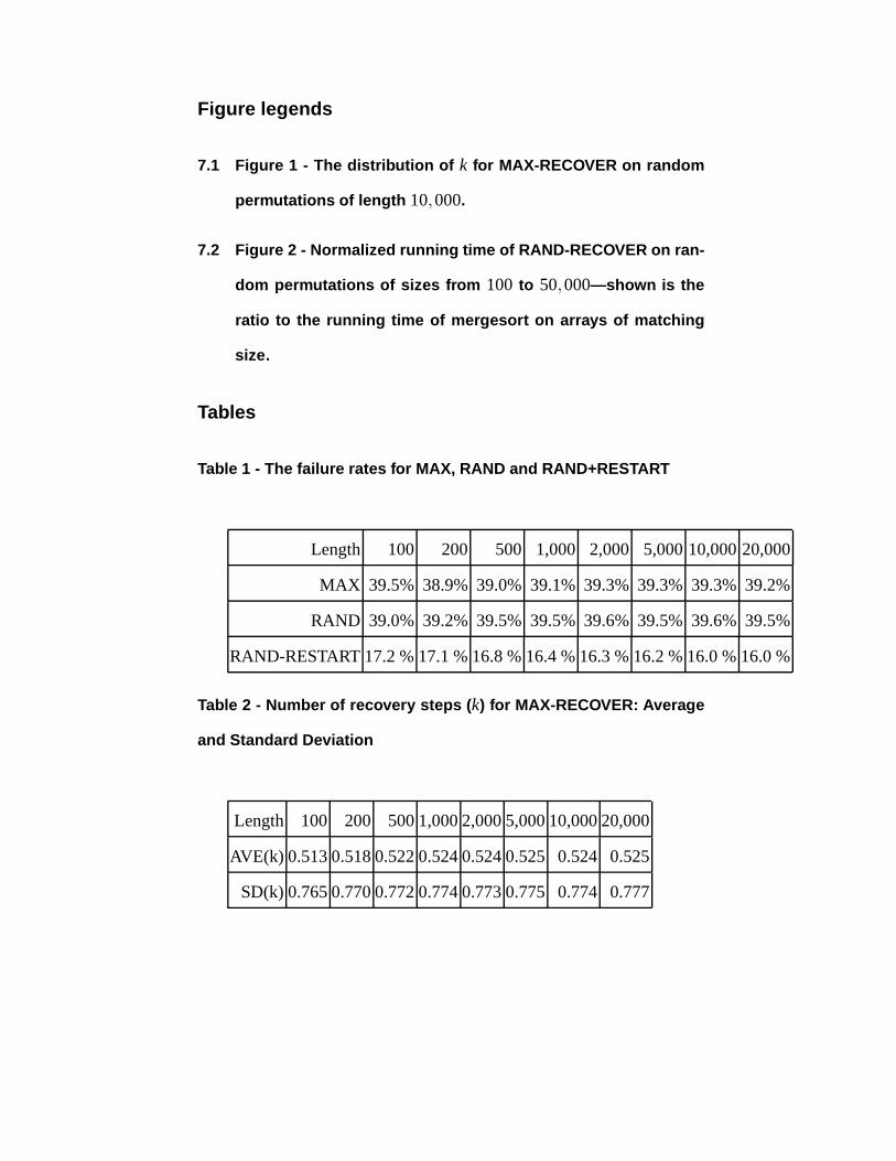
Figure legends

7.1 Figure 1 - The distribution of k for MAX-RECOVER on random

permutations of length 10,000.

7.2 Figure 2 - Normalized running time of RAND-RECOVER on ran -

dom permutations of sizes from 100 to 50,000—shown is the

ratio to the running time of mergesort on arrays of matching

size.

Tables

Table 1 - The failure rates for MAX, RAND and RAND+RESTART

Length 100 200 500 1,000 2,000 5,00010,00020,000

MAX 39.5% 38.9% 39.0% 39.1% 39.3% 39.3% 39.3% 39.2%

RAND 39.0% 39.2% 39.5% 39.5% 39.6% 39.5% 39.6% 39.5%

RAND-RESTART17.2 %17.1 %16.8 %16.4 %16.3 %16.2 %16.0 %16.0 %

Table 2 - Number of recovery steps ( k) for MAX-RECOVER: Average

and Standard Deviation

Length 100 200 5001,0002,0005,00010,00020,000

AVE(k) 0.5130.5180.5220.5240.5240.525 0.524 0.525

SD(k)0.7650.7700.7720.7740.7730.775 0.774 0.777

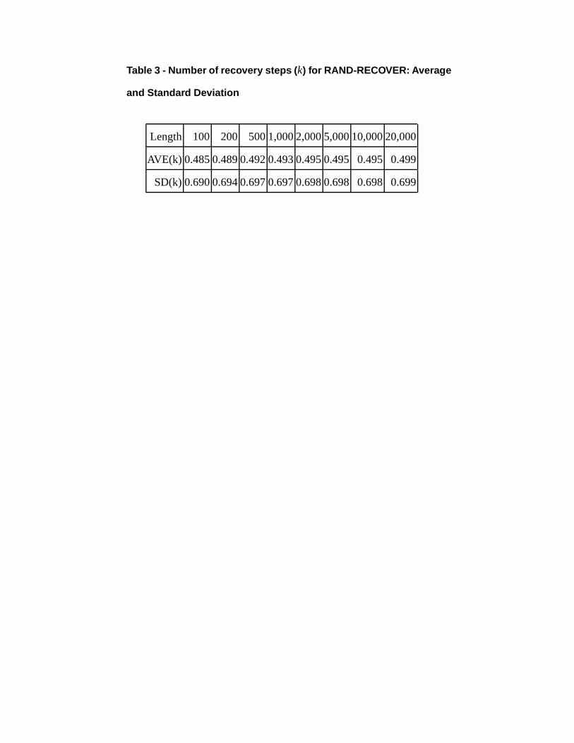
Table 3 - Number of recovery steps ( k) for RAND-RECOVER: Average

and Standard Deviation

Length 100 200 5001,0002,0005,00010,00020,000

AVE(k) 0.4850.4890.4920.4930.4950.495 0.495 0.499

SD(k)0.6900.6940.6970.6970.6980.698 0.698 0.699