EPA/600/R-99/030

Chapter 6

GOVERNING EQUATIONS AND COMPUTATIONAL STRUCTURE OF THECOMMUNITY MULTISCALE AIR QUALITY (CMAQ) CHEMICAL TRANSPORT

MODEL

Daewon W. Byun* and Jeffrey Young**

Atmospheric Modeling Division,National Exposure Research LaboratoryU.S. Environmental Protection Agency

Research Triangle Park, NC 27711

M. Talat Odman***

MCNC-Environmental ProgramsP.O. Box 12889, 3021 Cornwallis Road

Research Triangle Park, NC 27709-2889, USA

ABSTRACT

The chemical transport model (CTM) of the Models-3/CMAQ (Community Multiscale AirQuality) modeling system can be configured to follow the dynamics of the preprocessormeteorological model. A science process module in the CMAQ CTM is not specific to acoordinate system. The generality is accomplished through the use of the coordinatetransformation Jacobian within the CMAQ CTM. In this chapter, we derive the governingdiffusion equation in a generalized coordinate system, which is suitable for multiscaleatmospheric applications. We describe the CMAQ systemÕs modularity concepts, fractionaltime-step formulation, and key science processes implemented in the current version of theCMAQ CTM. We examine dynamic formulations of several popular Eulerian air quality modelsas emulated by the governing diffusion equations in the generalized coordinate system. Also, anesting technique for the CMAQ CTM is introduced. Finally, because the amount of asubstance in the atmosphere can be expressed in many different ways, we summarize the mostpopular expressions for concentration and their transformation relations.

*On assignment from the National Oceanic and Atmospheric Administration, U.S. Department of Commerce.Corresponding author address: Daewon W. Byun, MD-80, Research Triangle Park, NC 27711.E-mail: bdx@hpcc.epa.gov** On assignment from the National Oceanic and Atmospheric Administration, U.S. Department of Commerce.*** Present Affiliation: Georgia Institute of Technology, Atlanta, GA.

EPA/600/R-99/030

6-1

6.0 GOVERNING EQUATIONS AND COMPUTATIONAL STRUCTURE OF THECOMMUNITY MULTISCALE AIR QUALITY (CMAQ) CHEMICAL TRANSPORTMODEL

In Chapter 5, ÒFundamentals of Atmospheric Modeling ...Ó we discussed the fundamental set ofequations for atmospheric dynamics and thermodynamics in a generalized coordinate system. Inthis Chapter, we investigate the diffusion equation for the trace species in the atmosphere in thegeneralized coordinate system and the computational structure of the Community Multiscale AirQuality chemical transport model (CMAQ CTM or, hereafter, CCTM).

One requirement of the CMAQ modeling system is to maintain a consistent description of theatmosphere for different meteorological and chemical transport models. This is a feature that isessential for spatial scalability. Various coordinate systems are used in atmospheric models.Selection of a suitable coordinate system is an important step of model formulation. There arenumerous criteria to be considered in selecting a coordinate system, such as the dynamiccharacteristics it can handle and how well it can deal with curvature of the earthÕs surface andfeatures of the terrain. Formulation of the models may vary substantially for different coordinatesystems. If a CTM can be formulated and coded using a generalized coordinate system, it wouldbe easy to switch from one coordinate to another depending on the application. The generalizedcoordinate concept is useful because a single CTM formulation can adapt to any of thecoordinates commonly used in meteorological models. It is also desirable to compare the benefitsof various coordinate systems and to be able to link the CTMs to meteorological models anddatabases in different coordinates.

Conformity of the coordinates to the physics of the problem is very important. Unlike a modelwith a fixed coordinate system, a generalized coordinate system allows use of generic coordinatesfor the specific science processes within a model. Although the modelÕs overall structure isdetermined by the choice of a coordinate system, the individual science modules can still use theirown generic coordinates that best suit the physical processes they model. This means that eachscience process can utilize the parameterizations based on the best coordinate to represent theproblem. For example, the planetary boundary layer (PBL) parameterizations can be expressedin terms of geometric height, or dimensionless height scaled with PBL height, while for cloudphysics, they can be represented in terms of pressure. The linkages between the genericcoordinate parameterizations in the science processes and the governing conservation equation inthe generalized coordinates are established through the application of appropriate coordinatetransformation rules.

Here, we intend to provide a comprehensive and rational development of the governingconservation equation in generalized coordinates, which can be readily implemented in an Eulerianmodel. The operating assumptions used for the derivations are listed below (see Srivastava et al.,1995).

• Assumption 1: Pollutant concentrations are sufficiently small, such that their presencewould not affect the meteorology to any detectable extent. Hence, the species

EPA/600/R-99/030

6-2

conservation equations can be solved independently of the Navier-Stokes and energyequations. The conditions which could invalidate this assumption are for cases wheresufficient heat is generated by chemical reactions to influence the temperature of themedium or where an atmospheric layer become so concentrated with pollutants thatabsorption, reflection, and scattering of radiation alter the air flow (Seinfeld, 1986).

• Assumption 2: The velocities and concentrations of the various species in atmosphericflow are turbulent quantities and undergo turbulent diffusion. Because turbulent diffusionis much greater than molecular diffusion for most trace species, the latter can be ignored.

• Assumption 3: The metric tensor that defines the coordinate transformation rules is not aturbulent variable. This means that we can define the coordinates based on the Reynoldsaveraged quantities. The vertical grids will be defined incrementally between time stepswhen a time-dependent vertical coordinate is used.

• Assumption 4: The ergodic hypothesis holds for the ensemble averaging process. Thismeans that the ensemble average of a property can be substituted with the time average ofthat property.

• Assumption 5: The turbulence is assumed stationary for the averaging time period ofinterest (say 30 minutes to one hour for atmospheic applications).

• Assumption 6: The source function (i.e., emissions of pollutants) is deterministic for allpractical purposes and there is no turbulent component.

• Assumption 7: The effect of concentration fluctuation on the rate of chemical reaction isnegligible, i.e., contributions of covariance effects among tracer species are neglected.

• Assumption 8: Because the large-scale motions of the atmosphere are quasi-horizontalwith respect to the earth's surface, science processes can be separately represented inhorizontal and vertical directions (i.e., quasi-orthogonal in transformed coordinates).

6.1 Derivation of the Atmospheric Diffusion Equation

In Chapter 5, we derived the species continuity equation in generalized coordinates. It is givenas:

∂ ϕ∂

ϕ ∂ ϕ∂ ϕ

( ) ˆ ( ˙)i ss

i s s i ss

J

tm

J

m

J s

sJ Q

i+ ∇ •

+ =2

2

V(6-1)

where ϕ i is the trace species concentration in density units (e.g., kg m-3), Js is the vertical

Jacobian of the terrain-influenced coordinate s, m is the map scale factor, ˆ V s and s& are horizontal

and vertical wind components in the generalized coordinates, and iQϕ is the source or sink term.

EPA/600/R-99/030

6-3

To make the instantaneous species continuity equation useful for air quality simulation, we needto derive the governing diffusion equation. This is done by decomposing the variables inEquation 6-1, except for the Jacobian and map scale factor, in terms of mean and turbulentcomponents. The Reynolds decompositions of species concentration and mixing ratio areexpressed as:

ϕ ϕ ϕi i i= + " (6-2a)

q q qi i i= + " (6-2b)

ϕ ϕ ρ ρ ρ ρi i i i i iq q q q+ = + + +" " " " " (6-2c)

where qii= ϕ

ρ is the species mass mixing ratio and a stochastic quantity is decomposed into

mean , ( ), and turbulent, ("), components. Stationary turbulence assumption 5 implies that aturbulent component has a zero mean for the averaging period. Following Venkatram (1993), wecan estimate the mean and turbulent components of species and air concentrations as

ϕ ρi iq≈ (6-3a)

ϕ ρ ρ ρi i i iq q q" " " " "= + + (6-3b)

q

qi

i

" " "( )

ρρ

ρρ

≈ <<2

2 1 (6-3c)

Without loss of generality, we redefine the terrain-influenced vertical coordinate s with acoordinate ̂x 3 , whose value is increasing monotonically with height, as:

ˆ( )

( )x

s if s increases with height

s if s decreases with height3

1= =

−

ξ (6-4)

The choice of a generalized vertical coordinate which increases monotonically with heightsimplifies the derivation of the governing equation and thus reduces the likelihood of making signerrors in the formulas and in computer codes. The transformation does not change the horizontalwind components or the Jacobian, which is always defined to be a positive quantity. Hereafter,the subscript s is replaced with ξ to reflect modification of the vertical coordinate. Subsequently,

the vertical velocity is represented with ˆ / ˙v d dt3 = =ξ ξ , which is positive for upward motion.

Application of decomposition of velocity components in Equation 6-1 and ensemble averagingproduces Reynolds flux terms in the mass conservation equation as:

EPA/600/R-99/030

6-4

∂ ϕ∂

ϕ ϕξξ

ξ ξ ξ( ) ( ")( ˆ ˆ ")i i iJ

tm

J

m+ ∇ •

+ +

22

V V

+ + +

=∂∂

ϕ ϕ ξ ξ ϕˆ( ")( ˆ ˆ ")

xv v J J Qi i i3

3 3 (6-5)

where we used J Jξ ξ= and Q Qi iϕ ϕ= based on Assumption 3 and Assumption 6, respectively.

The Reynolds flux terms in Equation 6-5 can be approximated in terms of the mixing ratio as:

ϕ ρ ρ ρξ ξ ξ ξi i i iq q q" ˆ " " ˆ " " ˆ " " ˆ "V V V V≈ + ≈ (6-6a)

ϕ ρ ρ ρi i i iv q v q v q v" ˆ " " ˆ " " ˆ " " ˆ "3 3 3 3≈ + ≈ (6-6b)

qi ρ ξ" ˆ "V << 1 (6-6c)

q vi ρ" ˆ "3 1<< (6-6d)

in which we have neglected the second order perturbation terms based on the scale analysis of theequations. Equation 6-5 can be rewritten using Equations 6-3a-c and 6-6a-c to give:

∂ ϕ∂

ϕ ∂ ϕ∂

ξξ

ξ ξ ξ( ) ˆ ( ˆ )

ˆi i iJ

tm

J

m

v J

x+ ∇ •

+2

2

3

3

V

+ ∇ •

+ =m

q J

m

q v J

xJ Qi i

i

22

3

3ξξ ξ ξ

ξ ϕρ∂ ρ

∂" ˆ " ( " ˆ " )

ˆ

V(6-7)

The turbulence flux terms can be parameterized using a simple closure scheme such as the eddydiffusion concept (K-theory):

q u Kq

xil i

l" ˆ " ˆˆξ

∂∂

= − 1 ; q v Kq

xil i

l" ˆ " ˆˆξ

∂∂

= − 2 ; q v Kq

xil i

l" ˆ " ˆˆ

3 3= − ∂∂

(6-8)

where K̂ jl denotes the eddy diffusivity tensor in the transformed coordinate. The eddydiffusivity tensor for the generalized meteorological coordinates is related to the diffusivitytensor in Cartesian coordinates as:

ˆ ˆ ˆK

x

x

x

xKkl

k

i

l

jij= ∂

∂∂∂

(6-9)

EPA/600/R-99/030

6-5

If we postulate that the diffusivity tensor in Cartesian coordinates is diagonal (i.e., all the off-diagonal components vanish), then the eddy diffusivity tensor in the generalized meteorologicalcoordinates becomes:

ˆ

ˆ

ˆ

ˆ ˆ(

ˆ) (

ˆ) (

ˆ)

K =

+ +

m K mx

xK

m K mx

yK

mx

xK m

x

yK

x

xK

x

yK

x

zK

xx xx

yy yy

xx yy xx yy zz

23

23

3 3 32

32

32

0

0

∂∂∂∂

∂∂

∂∂

∂∂

∂∂

∂∂

(6-10)

where K Kxx = 11 , K Kyy = 22 , and K Kzz = 33 are the diagonal components of eddy

diffusivity tensor in the Cartesian coordinate. To match with the computational grid, the gradientterms in Equation 6-10 must be rewritten in terms of the generalized coordinates x̂3 (definedbased on height above ground h h zAGL sfc= − , where zsfc represents the height of topography)

using the appropriate chain rules, for example, 1

1 3 13 3m

A

x

A

x

A

z

A

x

h

xz x x

∂∂

∂∂

∂∂

∂∂

∂∂

=

−

ˆ ˆ ˆˆ ˆ

. When A

= x̂3 , we get

ˆ

ˆˆ

ˆˆ

ˆˆ

ˆˆ

(ˆ

)ˆ ˆ

K =

−

−

− −

+

m K mx

z

h

xK

m K mx

z

h

xK

mx

z

h

xK m

x

z

h

xK

x

zm

h

xK m

h

x

xx xx

yy yy

xx yy xx

2 23

1

2 23

2

23

12

3

2

32

1

2

2

0

0

∂∂

∂∂

∂∂

∂∂

∂∂

∂∂

∂∂

∂∂

∂∂

∂∂

∂∂

+

2

K Kyy zz

(6-11).

Then the non-zero diffusion terms in Equation 6-7 can be parameterized with the eddy diffusiontheory as follows:

mq J

mm

x

J

mK

q

xK

q

xi i i2

22

1 211

113

3∇ •

= − +

ξξ ξ ξρ ∂

∂ρ ∂

∂∂∂

" ˆ "

ˆ( ˆ

ˆˆ

ˆ)

V

+ − +

mx

J

mK

q

xK

q

xi i2

2 222

223

3

∂∂

ρ ∂∂

∂∂

ξ

ˆ( ˆ

ˆˆ

ˆ) (6-12)

and

∂ ρ∂

∂∂

ρ ∂∂

∂∂

∂∂

ξξ

( " ˆ " )

ˆ ˆ( ˆ

ˆˆ

ˆˆ

ˆ)

q v J

x xJ K

q

xK

q

xK

q

xi i i i

3

3 331

132

233

3= − + +

(6-13)

EPA/600/R-99/030

6-6

Rewriting Equation 6-7 with Equations 6-12 and 6-13, and separating the diagonal and off-diagonal diffusion terms with an explicit description of the source terms, one can obtain thegoverning atmospheric diffusion equation in the generalized coordinates where the turbulent fluxterms are expressed with the eddy diffusion theory:

∂ ϕ∂

ϕ ∂ ϕ∂

ξξ

ξ ξ ξ( ) ˆ ( ˆ )

ˆi i iJ

tm

J

m

v J

x+ ∇ •

+2

2

3

3

V

(a) (b) (c)

−

−

mx

J

mK

q

xm

x

J

mK

q

xi i2

1 211

12

2 222

2

∂∂

ρ ∂∂

∂∂

ρ ∂∂

ξ ξ

ˆ( ˆ

ˆ)

ˆ( ˆ

ˆ) −

∂∂

ρ ∂∂ξˆ

( ˆˆ

)x

J Kq

xi

333

3

(d) (e)

−

−

mx

J

mK

q

xm

x

J

mK

q

xi i2

1 213

32

2 223

3

∂∂

ρ ∂∂

∂∂

ρ ∂∂

ξ ξ

ˆ( ˆ

ˆ)

ˆ( ˆ

ˆ)

(f)

− +

∂∂

ρ ∂∂

∂∂ξˆ

( ˆˆ

ˆˆ

)x

J Kq

xK

q

xi i

331

132

2

(g)

= + + + +J R J QJ

t

J

t

J

ti iNi

cld

i

aero

i

ping

ξ ϕ ξ ϕξ ξ ξϕ ϕ

∂ ϕ∂

∂ ϕ∂

∂ ϕ∂

( ,..., )( ) ( ) ( )

1 (6-14)

(h) (i) (j) (k) (l)

The terms in Equation 6-14 are summarized as follows:

(a) time rate of change of pollutant concentration;(b) horizontal advection;(c) vertical advection;(d) horizontal eddy diffusion (diagonal term);(e) vertical eddy diffusion (diagonal term);(f) off-diagonal horizontal diffusion;(g) off-diagonal vertical diffusion;(h) production or loss from chemical reactions;(i) emissions;(j) cloud mixing and aqueous-phase chemical production or loss;(k) aerosol process; and

EPA/600/R-99/030

6-7

(l) plume-in-grid process.

Note that the dry deposition process can be included in the vertical diffusion process as a fluxboundary condition at the bottom of the model layer.

Alternatively, we can express the turbulent flux terms in Equation 6-7 using the Reynolds fluxterms defined as:

q u Fi qi" ˆ " ˆ

ξ = 1 , q v Fi qi" ˆ " ˆ

ξ = 2 , q v Fi qi" ˆ " ˆ3 3= (6-15)

and the turbulent flux terms are related with the Cartesian counterpart using ˆ ˆF

x

xFq

kk

j qj

i i= ∂

∂:

F̂ mFq qx

i i

1 = , F̂ mFq qy

i i

2 = , ˆ (ˆ

) (ˆ

) (ˆ

)Fx

xF

x

yF

x

zFq q

xqy

qz

i i i i

33 3 3

= + +∂∂

∂∂

∂∂

(6-16)

In comparison with Equation 6-14, the Reynolds flux terms shown in Equation 6-15 include theoff-diagonal components. One can now rewrite the governing conservation equation for tracespecies equivalently to Equation 6-14 in terms of the Reynolds flux terms:

∂ ϕ∂

ϕ ∂ ϕ∂

ξξ

ξ ξ ξ( ) ˆ ( ˆ )

ˆi i iJ

tm

J

m

v J

x+ ∇ •

+2

2

3

3

V

+

+

+ [ ]mx

J

mF m

x

J

mF

xJ Fq q qi i i

21 2

1 22 2

23

3∂∂

ρ ∂∂

ρ ∂∂

ρξ ξξˆ

ˆˆ

ˆˆ

ˆ

= + + + +J R J QJ

t

J

t

J

ti iNi

cld

i

aero

i

ping

ξ ϕ ξ ϕξ ξ ξϕ ϕ

∂ ϕ∂

∂ ϕ∂

∂ ϕ∂

( ,..., )( ) ( ) ( )

1 (6-17)

The governing equation can be simplified for a domain with gentle topography for which one mayignore all the terms involved with the horizontal gradients of the surface normal to the verticalcoordinate. This forces the vertical diffusion terms in the curvilinear coordinate system to beidentical to those of the orthogonal Cartesian coordinate system. Then the trace speciesconservation equation can be written in a simpler form:

∂ϕ∂

ϕ ∂ ϕ∂

ρ γ∂ ρ γ

∂ξ ξ ξi

ii

qq

t

v

x

F

xi

i

**

*ˆ ˆ ( ˆ )

ˆˆ ˆ ˆ ( ˆ ˆ )

ˆ+ ∇ •[ ] + + ∇ •[ ] +V F

3

3

3

3

= + + + +ˆ ( ,..., ) ˆ ( ) ( ) ( )* * *

γ ϕ ϕ γ ∂ ϕ∂

∂ ϕ∂

∂ ϕ∂ϕ ϕR S

t t ti iNi

cld

i

ping

i

aero

1 (6-18)

EPA/600/R-99/030

6-8

whereϕ γ ϕ ϕξi i iJ m* ˆ ( / )= = 2 . In writing Equation 6-18, we have explicitly identified terms to

directly relate to science process modules implemented in the CMAQ. Equation 6-18 is similarto the conservation equation in the generalized coordinates as suggested by Toon et al. (1988).

6.2 Representation of Science Processes in CMAQ Modeling System

This section describes how the CMAQ modeling system is structured to accommodate manydifferent science process modules that provide a one-atmosphere, multiscale and multi-pollutantmodeling capability to the CMAQ system. First, we describe the modularity concepts and keyscience processes implemented in the current version of CMAQ. Then the governing fractionaltime-step formulation for each science process is presented.

6.2.1 Supporting Models and Interface Processors

Key supporting models for the current version of the CMAQ modeling system are theMesoscale Model Version 5 (MM5) (Seaman et al., 1995)and Models-3 Emissions Processingand Projection System (MEPPS). The CMAQ modeling system is comprised of the mainCMAQ chemical transport model (CCTM) and several interface processors that link other modelinput data to the CCTM. The Meteorology-Chemistry Interface Processor (MCIP) processesMM5 output to provide a complete set of meteorological data required for CCTM. MCIP isdesigned in such a way that other meteorological models can be linked with minimal effort. Initialand boundary conditions are generated with the ICON and BCON processors, respectively, andthe Emissions-Chemistry Interface Processor (ECIP) combines area and point source emissionsto generate three-dimensional gridded emissions data for CCTM. In addition, a plume dynamicsmodel (PDM) is used to provide dimensions and positions of plumes from major elevated point-sources. The PDM data are used for driving the plume-in-grid processing in CCTM. Aphotolytic rate constant processor (JPROC) which is based on the RADM (Chang et al., 1987)approach, computes species specific photolysis rates for a set of predefined zenith angles,latitude, and altitudes. An alternative detailed-science version adopts state-of-the-scienceradiative transfer models that can take into account the total ozone column (TOMS data) andturbidity. Refer to Table 6-1 for the list of the interface processors in CMAQ and Figure 6-1 forthe data linkage among these interface processors.

By assembling appropriate science modules available in the CMAQ system, users can build aspecific CCTMÕs that may include all or some of the critical science processes, such asatmospheric transport, deposition, cloud mixing, emissions, gas- and aqueous-phase chemicaltransformations, and aerosol dynamics and chemistry. One of the features of CMAQ thatdistinguishes it from other air quality models is the hierarchical functional modularity of thescience processor codes. We define the levels of modularity in the science model based on thegranularity of the modeling components. The coarsest level of modularity is the distinctionbetween the system framework and science models. The second level is the division of sciencesub-models (MM5, MEPPS, and CMAQ). The third level of modularity involves a drivermodule, processor modules, data provider modules, and a utility module (a collection of assisting

EPA/600/R-99/030

6-9

subroutines) in a CTM. While the emissions processing and the meteorology model are modularat the second level, the CCTM achieves the third-level of modularity by employing the operatorsplitting, or fractional time step, concept in the science processes. The next level of modularityis based on the computational functionality in a processor module, e.g., science parameterization,numerical solver, processor analysis, and input/output routines. The lowest meaningfulmodularization level is the isolation of sections of code that can benefit from machine dependentoptimization.

6.2.2 Modularity Concept of CMAQ

To allow for both the continuous improvement of science and for the addition of new capabilitiesin a unified fashion, it is critical to have efficient modular schemes in the CMAQ design.Currently, the modularity within CMAQ is based mostly on the fractional time-stepimplementation of the science processes. This level of modularity involves the distinction of adriver, processor modules, data provider modules, and utility subroutines in CMAQ. We havechosen this method because it provides a natural disciplinary distinction for different scienceprocesses through which developments in specific research areas can readily be incorporated(Refer to Figure 6-2).

In some of the process modules, such as the aqueous-phase chemistry module, the sciencealgorithms and numerical solvers are tightly linked. For other types of modules, the scienceparameterization components and numerical solvers have a looser association. In such cases themodularity can be defined either at the parameterization level, the numerical algorithm level, orboth. For example, the module definition for the advection process is based on the numericaladvection algorithm used. For the gas-phase chemistry process, the modularity is based on theordinary differential equation numerical solvers. The chemistry mechanism description isgeneralized and the Models-3/CMAQ framework provides a straightforward method to linkmodel species surrogate names with the species names in the data set. See Chapter 15 for details.The use of different chemical mechanisms is accommodated through the mechanism reader andgeneralized codes for setting up the production and loss terms of the chemistry reactions.Therefore, the CCTM does not require different gas-phase chemistry modules for differentmechanisms.

The vertical diffusion process can be formulated using either local- or non-local-mixingparameterization schemes. The current classification of vertical diffusion modules is based on theprocess parameterization methods. The modularity of this process can be enhanced if wedistinguish the method used for computing the vertical diffusivities for local-mixing. In this case,the modularity is defined at the level of data provider modules. The modularity level can bedeepened further if we identify different numerical solution methods for the diffusion.

With the current version of CMAQ, the level of science modularity is subordinated by the waythe science process codes are archived in the system. Here, we define a class as a collection ofdifferent modules for a given science process. The science classes are identified with the grouping

EPA/600/R-99/030

6-10

of the terms in the governing conservation equation, Equation 6-18. Currently, nine scienceprocess classes are defined in CCTM:

• DRIVER controls model data flows and synchronizes fractional time steps;

• HADV computes the effects of horizontal advection;

• VADV computes the effects of vertical advection;

• ADJCON adjusts mixing ratio conservation property of advection processes;

• HDIFF computes the effects of horizontal diffusion;

• VDIFF computes the effects of vertical diffusion and deposition;

• CHEM computes the effects of gas-phase chemical reactions;

• CLOUD computes the effects of aqueous-phase reactions and cloud mixing;

• AERO computes aerosol dynamics and size distributions; and

• PING computes the effects of plume chemistry.

CCTM does not have emissions as a separate science process because it can be either a part ofthe vertical diffusion or the gas-phase chemical reaction process. It is worthwhile to mentionhere that the current modular paradigm does not prevent establishment of combination ofprocesses in a larger single module. For example, one can develop a module describing the verticaltransport, chemistry, and emissions simultaneously when time scales of those processes becomecomparable. Users could experiment with the combination of modules to best fit to theirproblems at hand.

In addition to nine science process modules, CCTM includes two science process classes. ThePHOT computes photolysis rates, and AERO_DEPV computes particle size-dependent drydeposition velocities. These are typical Òdata-providerÓ science process classes, which do notinvolve updating concentrations directly. There are some other classes that do not fall in any ofthe above definitions. We have grouped these auxiliary routines as the UTIL class, which is acollection of utility subroutines. As one can see, the current modularity of the CCTM isimplemented more on a practical basis rather than by strictly following a design paradigm. Onecan also see that the present modularity definition of CMAQ is somewhat subjective. In thefuture we intend to allow definition of the modularity at the user-defined granularity level.

Figure 6-1 describes the key science process modules in CCTM and their data linkage withCMAQÕs preprocessors, whose descriptions are available in other chapters. The only datadependencies among the CCTM science modules are the trace species concentration field as seenin the diagram and the model integration time step. Figure 6-2 shows the distinct data

EPA/600/R-99/030

6-11

dependencies within the CCTM. To facilitate modularity and to minimize data dependency inCCTM, we store concentrations in global memory while the environmental input data areobtained from random-access files and interpolated to the appropriate computational(synchronization) time step. This realizes the recommended Òthin-interfaceÓ structure of themodel:

• Common timing data are managed through the science process main subroutineÕs callarguments;

• Concentrations are the object of all process operations;

• Environmental data are provided through a standard I/O interface;

• Model structure data are provided through shared include files; and

• Standard physical constants are obtained from shared include files.

See Chapter 18 for further details on how the science codes are integrated in the Models-3CMAQ system.

EPA/600/R-99/030

6-12

CMAQDriver

Couple/Decouple

Vert.Diffusion

Horiz.

Diffusion

Gas-PhaseChemistry

Aerosol

AqueousChemistry &

CloudDynamics

Plumein Grid

Init

ConcentrationMeteorology

Emissions

ICON

PDM

JPROC

MCIP

ECIP

BCON

Horiz.Advection

Vert.Advection

Photoliticrates

Plume Dynamics

BoundaryConditions

InitialConditions

Output Files

CMAQ Science Processors

Figure 6-1. Science Process Modules in CMAQ. Interface processes are shown with rectangularboxes. Typical science process modules are updating the concentration field directly and the data-provider modules include routines to feed appropriate environmental input data to the scienceprocess modules. Driver module orchestrates the synchronization of numerical integration acrossthe science processes. Concentrations are linked with solid lines and other environmental data withbroken lines. (From Byun et al., 1998.)

EPA/600/R-99/030

6-13

Table 6-1. Interface Processors for the CMAQ Modeling System

InterfaceProcessor

Description Reference

ICON Provides initial three-dimensional fields of trace speciesconcentrations for modeling domain

Chapter 13

BCON Provides concentrations of trace species for the boundarycells

Chapter 13

ECIP Incorporates emissions from separate area and majorpoint sources to generate hourly 3-D emissions input file

Chapter 3

MCIP Processes the output of a meteorological model toprovide the necessary meteorological data for CMAQmodels

Chapter 12

JPROC Computes photolysis rates for various altitudes,latitudes, and sun zenith angle

Chapter 14

PDM Generates plume information needed to apply plume-in-grid (PinG) processing in CCTM

Chapter 9

EPA/600/R-99/030

6-14

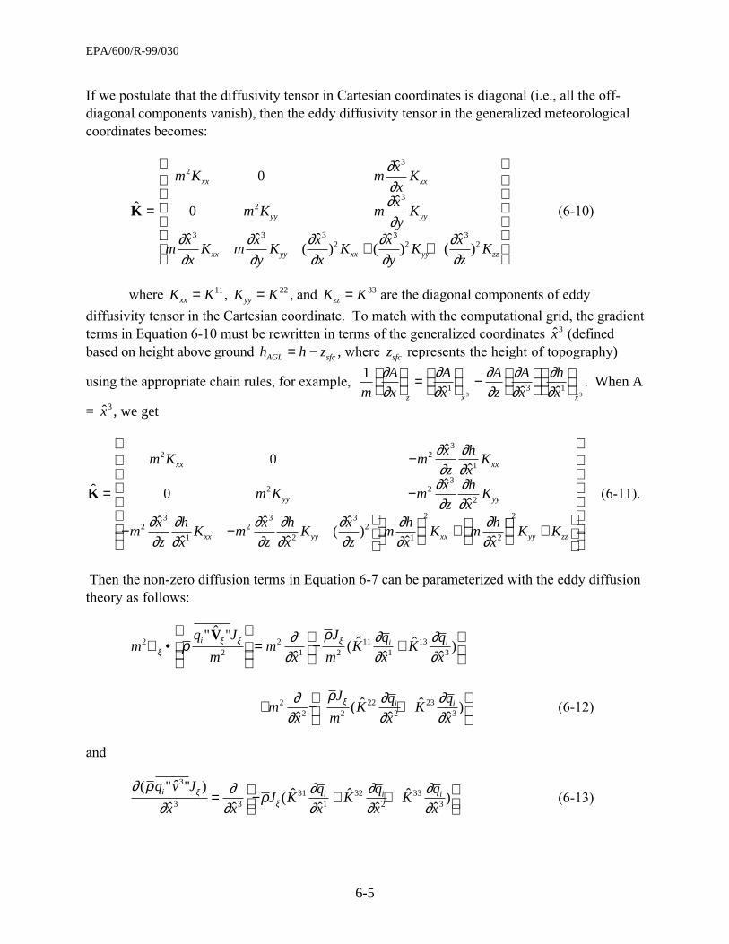
6.2.3 Description of Science Processes

In this section we describe individual science processes, shown in Figure 6-1, associated with thegroups of individual terms in the governing diffusion equation. Note that different concentrationunits are used for different science processes in CMAQ CTMs. Appendix 6A provides therelationships among the concentration units and their conversion factors from one unit to another.

OutputPN

P1 •••••

Input(once)

P2

P3

Sk

Sk

Sk

Sk

Random-Access Disk File

Global Memory(Concentration)

LocalMemory

CMAQ CTM 's Data Flow

ICData

Environmental Data (Meteorology, Emissions, BC)

Figure 6-2. Data Dependencies Among Modules in CCTM. P and Sk represent a science processmodule and the related subroutines for the module, respectively. (From Byun et al., 1995.)

6.2.3.1 Driver Class for CCTM

The key function of the driver class module is hosting the science processors. It is responsiblefor coordinating model integration time (synchronizing fractional-time steps of science processcall) and some input/output sequences. The driver structure of the current CCTM is given inFigure 6-3. A synchronization time step is used to ensure the global stability of the CCTMÕsnumerical integration at the advection time step, which is based on a Courant number limit.Nesting requires finer synchronization time steps for the fine grid domain. The CCTMÕs processsynchronization time steps are represented as integer seconds because the Models-3 I/O API canonly handle integer seconds for I/O data. All the needed data are appropriately interpolatedbased on the synchronization time step. For maintaining numerical stability and for otherreasons, an individual process module may have its own internal time steps. In general, eachscience process module uses the synchronization time step ( ∆tsync ) as the input time step of

required environmental data. The global output time steps can be set differently from the

EPA/600/R-99/030

6-15

synchronization time step. Usually, the output time step ( ∆tout ) is set as one hour, but sub-

hourly output down to the synchronization time step is possible.

Table 6-2. List of Science Process Subroutines Called by the CMAQ Driver

Subroutine Science Class DescriptionCGRID_MAP UTIL Sets up pointers for different concentration species: gas

chemistry, aerosol, non-reactive, and tracer speciesINITSCEN INIT* Initializes simulation time period, time stepping constants, and

concentration arrays for the driverADVSTEP DRIVER Computes the model synchronization time step and number of

repetitions for the output time stepCOUPLE/DECOUPLE

COUPLE* Converts units and couples or de-couples concentration valueswith the density and Jacobian for transport

SCIPROC DRIVER Controls all of the physical and chemical processes for a grid(currently, two versions are available: symmetric andasymmetric around the chemistry processes)

XADV,YADV

HADV Computes advection in horizontal plane (x- and y-directions)

ZADV VADV Computes advection in the vertical direction in the generalizedcoordinate system

ADJADV ADJCON Adjusts concentration fields to ensure mixing ratioconservation given mass consistency error in meteorology data

HDIFF HDIFF Computes horizontal diffusionVDIFF VDIFF Computes vertical diffusion and depositionCHEM CHEM Solves gas-phase chemistryPING PING Computes effects of plume-in-grid processAERO AERO Computes aerosol dynamics, particle formation, and

depositionCLDPRC CLOUD Computes cloud mixing and aqueous chemistry*represents a process class that is part of DRIVER function.

EPA/600/R-99/030

6-16

XADV

YADV

ZADV

ADJCON

HDIFF

VDIFF

CHEM

AERO

CLDPRC

COUPLE

VDIFF

PING

HDIFF

ZADV

YADV

XADV

ADJCON

Symmetric SCIPROC

DECOUPLE

∆tsync

∆tsync / 2

DECOUPLE

XADV*

YADV*

ZADV

ADJCON

HDIFF

DECOUPLE

VDIFF

CHEM

AERO

CLDPRC

COUPLE

PING

Asymmetric SCIPROC

* AlternatingXADV and YADV callsfor each asymmetricSCIPROC call

CGRID_MAP

INITSCEN

ADVSTEP

COUPLE

SCIPROC

SynchronizationTime Step

OutputTime Step

CMAQ-DRIVER

∆tsync

∆tsync

∆tsync

∆tout

Figure 6-3. Driver Module and Its Science Process Call Sequence.Both asymmetric and symmetric call sequences in SCIPROC are presented. ∆tsync and ∆tout are

model synchronization and output time steps, respectively. Refer to Table 6-2 for the descriptionof the subroutines.

The DRIVER program calls initialization routines to set up CCTM runs. It initializes theconcentration field and checks if the input files, run time, and grid/coordinate information areconsistent for a given scenario. Subroutines used for the initialization process are grouped intothe INIT class. Usually, initial concentrations for gaseous species are in molar mixing ratio units(ppm) and aerosol species in density units (µg m-3), the same as the output units of CMAQ.Also, DRIVER calls couple/decouple subroutines to convert concentration units for appropriatedata processing. The pair of couple/decouple calls, which are available in the class COUPLE,limit the interchange of process modules between two different concentration units, such asdensity versus mixing ratio. The classes INIT and COUPLE are introduced just for the

EPA/600/R-99/030

6-17

convenience of code management from the point of view of science process modularity, and theyshould be considered as part of the DRIVER class modules.

6.2.3.2 Advection Processes for CCTM: HADV, VADV and ADJCON

For convenience, the advection process is divided into horizontal and vertical components. Thisdistinction is possible because the mean atmospheric motion is mostly in horizontal planes.Usually the vertical motion is related with the interaction of dynamics and thermodynamics. Theadvection process relies on the mass conservation characteristics of the continuity equation:

∂ γ ϕ∂

γ ϕ∂ γ ϕ

∂ξ ξ( ˆ ) ˆ ˆ ( ˆ ˆ )

ˆi

ii

t

v

x= −∇ • ( ) −V

3

3 (6-19)

Using the dynamically and thermodynamically consistent meteorology data from MCIP, we canmaintain data consistency for air quality simulations at the synchronization time step. In casethe meteorological data provided and the numerical advection algorithms are not exactly massconsistent, we need to solve a modified advection equation:

∂ γ ϕ∂

γ ϕ∂ γ ϕ

∂ϕ γ

ρξ ξρ( ˆ ) ˆ ˆ ( ˆ ˆ )

ˆˆi

ii

it

v

x

Q= −∇ • ( ) − +V

3

3 (6-20)

where Qρ is mass consistency error term (Byun, 1999). Equation 6-20 ensures conservation of

mixing ratio, which is a necessary (though not sufficient) condition for preserving total tracermass given significant fluctuations of density field in space and time. The equation shows thatthe correction term has the same form as a first-order chemical reaction whose reaction rate isdetermined by the mass consistency error (normalized with air density) in the meteorology data.

Modules in HADV class solve for the horizontal advection:

∂ γ ϕ∂

γ ϕξ ξ( ˆ ) ˆ ˆi

it= −∇ • ( )V (6-21)

and modules in VADV class solve for the vertical advection with boundary conditions v̂3 0= atthe bottom and top of the model.

∂ γ ϕ∂

∂ γ ϕ∂

( ˆ ) ( ˆ ˆ )ˆ

i i

t

v

x= −

3

3 (6-22)

In simulating air quality, one of fundamental characteristic of the model application should beconservation of mass. Therefore, the modules in the ADJCON class solve for the masscorrection term:

∂ γ ϕ∂

ϕ γρ

ρ( ˆ ) ˆiit

Q= (6-23)

EPA/600/R-99/030

6-18

We wish to emphasize that the artificial distinction of advection modules between horizontal andvertical processes is not adequate and that all three modules (HADV, VADV, and ADJCON)should be considered as an integral unit for solving the physical advection process of tracespecies. The advection and mass adjustment algorithms are described in detail in Chapter 7.

6.2.3.3 Diffusion Process Classes for CCTM: HDIFF and VDIFF

For convenience the atmospheric diffusion process is divided into horizontal and verticalcomponents. This distinction is needed because the vertical diffusion mostly represents thethermodynamic influence on the atmospheric turbulence by the air-surface energy exchangeprocesses while the horizontal diffusion represents subgrid scale mixing due to the unresolvedwind fluctuations. To handle the atmospheric diffusion processes in the generalized coordinates,we need to carefully examine the governing equation to properly set up the diffusion solver.

We start from the atmospheric diffusion equation in the same concentration units as used inadvection:

∂ϕ∂

∂ γ ρ

∂γ ρ

∂ γ ρ∂

γ ρρϕi

diff

i

diff

s qq

t

q

t

F

x

Qi

i i

* ˆˆ ˆ ˆ ( ˆ ˆ )

ˆˆ=

( )= −∇ •[ ] − +

F3

3 (6-24)

where ϕ γ ϕi i* ˆ= , and the term (Qϕi

/ ρ ) is the time rate change of mass mixing ratio due to

emissions of species i. Initially, it is assumed that we can decompose the diffusion into thehorizontal and vertical components with respect to the curvilinear coordinates:

∂ϕ∂

∂ γ ρ

∂γ ρξ

i

hdiff

i

hdiff

qt

q

t i

* ˆˆ ˆ ˆ=

( )= −∇ •[ ]F (6-25)

∂ϕ∂

∂ γ ρ

∂∂ γ ρ

∂γ ρ

ρϕi

vdiff

i

vdiff

q

t

q

t

F

x

Qi i

* ˆ ( ˆ ˆ )

ˆˆ=

( )= − +

3

3 (6-26)

Emissions can be included either in vertical diffusion or gas-phase chemistry module. If we canparameterize the turbulent fluxes directly in the curvilinear coordinates, we can implementHDIFF and VDIFF modules following Equations 6-25 and 6-26. When the turbulent fluxes areparameterized with eddy diffusion theory, the contributions of the off-diagonal (cross-directional) diffusion terms show up explicitly as shown in Equation 6-14:

∂ϕ∂

∂∂

γ ρ ∂∂

∂∂

γ ρ ∂∂

i

cdiff

i i

t xK

q

x xK

q

x

*

ˆˆ ( ˆ

ˆ)

ˆˆ ( ˆ

ˆ)=

+

1

133 2

233

EPA/600/R-99/030

6-19

+ +

∂∂

γ ρ ∂∂

∂∂ˆ

ˆ ( ˆˆ

ˆˆ

)x

Kq

xK

q

xi i

331

132

2 (6-27)

For a domain with a significant topographic feature, the module CDIFF must be implemented.However, the current CMAQ version does not include CDIFF module as the off-diagonal termsare often neglected in operational air quality models. In such a case, the HDIFF and VDIFFmodules solve for diagonal terms (with respect to the curvilinear coordinates) as follows:

∂ϕ∂

∂∂

γ ρ ∂∂

∂∂

γ ρ ∂∂

i

hdiff

i i

t xK

q

x xK

q

x

*

ˆˆ ( ˆ

ˆ)

ˆˆ ( ˆ

ˆ)=

+

1

111 2

222 (6-25Õ)

∂ϕ∂

∂∂

γ ρ ∂∂

i

vdiff

i

t xK

q

x

*

ˆˆ ( ˆ

ˆ)=

3

333 (6-26Õ)

Compared with above formulations, letÕs consider the case that we approximate the quantityγ̂ ρ , which defines the computational grid, to be constant for the duration of synchronization

time step for integrating the diffusion process with the fractional time-step method. Then, theproblem becomes equivalent to solving for the diffusion equations in terms of the mass mixingratio instead of density:

∂∂

∂∂ ρξ

ϕq

t

F

x

Qi

diffq

q

i

i i= −∇ •[ ] − +

ˆ ˆ ( ˆ )

ˆF

3

3 − • ∇ [ ] −[ ]ˆ ˆ ln( ˆ ) ˆln( ˆ )

ˆFq qi i

Fxξ γ ρ

∂ γ ρ

∂3

3 (6-28)

If we rely on Equation 6-28 for representing the atmospheric diffusion process, the concentrationmust first be decoupled to obtain mass mixing ratio, qi. Once the new mixing ratio is computed, itneeds to be coupled with γ̂ ρ to give the updated concentration in terms of ϕ i

* . This means

that the operator for the horizontal diffusion process should compute:

∂∂

γ ρξ ξq

ti

hdiffq qi i

= −∇ •[ ] − • ∇ [ ]ˆ ˆ ˆ ˆ ln( ˆ )F F (6-29)

and the vertical diffusion process should solve for:

∂∂

∂∂ ρ

∂ γ ρ

∂ϕq

t

F

x

QF

xi

vdiff

qq

i i

i= − +

−[ ]( ˆ )

ˆˆ

ln( ˆ )

ˆ

3

33

3 (6-30)

This approach is more convenient in numerically solving the flux-form turbulence mixingrepresentation because most of the flux-based closure algorithms use parameterizations ofturbulent fluxes in terms of conserving quantities, such as the mass mixing ratio, qi. Aconsiderable amount of meteorological and air quality literature on turbulence diffusion fails toclarify this important point. Especially for the case of multiscale applications, the representationof diffusion in terms of a conserving quantity is critical as shown by Venkatram (1993).

EPA/600/R-99/030

6-20

The effects of turbulence flux caused by the divergence of the grid boxes in the coordinate systemneed to be included in order to describe the turbulence exchange processes precisely. One canreadily show that the coordinate-divergence term in Equation 6-30 vanishes for a mass conservingvertical coordinate. Similarly, when topographical features vary significantly and horizontalvariations of the quantity γ̂ ρ are large, one cannot neglect the last term in Equation 6-29.

Chapter 7 of this document describes physical parameterization schemes and numericalalgorithms for the horizontal and vertical diffusion processes in the CCTM.

One may wonder how deposition should be represented in the generalized coordinate system. InEulerian air quality models, the deposition process affects the concentration in the lowest layeras a boundary flux condition. Considering the deposition process as the diffusion flux at thebottom of the model, we can relate the boundary condition in the generalized coordinate systemto that of the Cartesian coordinate system as:

ˆ (ˆ

) (ˆ

) (ˆ

)Fx

xF

x

yF

x

zFq q

xqy

qz

i dep i dep i dep i dep

33 3 3

= + +∂∂

∂∂

∂∂

= (ˆ

)∂∂x

zFq

z

depi

3

(6-31)

because Fqx

depi and Fq

y

depi do not exist. Then, the effects of dry deposition on the species

concentration is accounted for by the following relationship:

∂ϕ∂

∂ γ ρ

∂∂ γ ρ

∂∂

∂γ ρ ∂

∂i

dep

i

dep

q

dep

qz

dept

q

t

F

x x

x

zFi

i

* ˆ ( ˆ ˆ )

ˆ ˆˆ (

ˆ)=

( )= − = −

3

3 3

3

≈ −− ( )

= − = −(

ˆ) ( ˆ )

( ˆ )( ˆ ) *

∂∂

γ ργ ρ ϕ

x

zF

x

v

hq

v

h

dep i dep

dep dep

layer

dep

layer

qz

di

di

3

3 1 1∆(6-32)

where hz

xx

dep

depdep=

∂∂ˆ

( ˆ )33∆ is the thickness of the lowest model layer in the geometric height

coordinate. In the derivation of Equation 6-32, we assume that the deposition flux is constant inthe lower part of the surface layer (i.e., a constant flux layer). Thus, the deposition velocities arecomputed at the middle (in terms of the generalized coordinate, ξ) of the lowest model layer atwhich the concentrations are represented. For the case in which the mass mixing ratio is used asthe concentration variable for solving the diffusion equation, the deposition should beimplemented as a boundary condition for the vertical diffusion (VDIFF) in the following manner:

∂∂

∂∂

∂∂

∂∂

q

t

F

x x

x

zFi

dep

q

dep

qz

dep

i

i= − = −

( ˆ )

ˆ ˆ(

ˆ)

3

3 3

3

(6-33)

Therefore, the bottom boundary condition for the VDIFF module is given as:

EPA/600/R-99/030

6-21

∂∂

∂∂

∂∂

q

t x

x

zFi

qz

depi

dep

= −

ˆ

(ˆ

)3

3

≈ −−

( )

=( )

= −

∂∂ˆ

( ˆ )

x

zF

x

F

h

v

hqbottom

i dep

dep

i dep

dep dep

layer

qz

qz

di

3

3 1∆(6-33Õ)

Equations 6-32 and 6-33 show that we do not need to estimate contravariant depositionvelocities if the deposition process is implemented as a bottom boundary condition in thegeneralized coordinate formulation.

In the current CCTM implementation, the concentration units for horizontal and vertical

diffusion processes are density (coupled with Jacobian) and molar mixing ratio, mi = qi

Mair

Mi

,

respectively. We have chosen mi as the generic concentration unit for the vertical diffusion to

coordinate with the emissions units in the data. Subsection 6.2.3.6 provides a detailedexplanation for this. Therefore, HDIFF is placed outside and VDIFF is placed in between thepair of couple/decouple calls. Because the ratio of molecular weights are constant, equations forthe vertical diffusion in terms of molar mixing ratio are equivalent to those in terms of massmixing ratio, qi . Refer to Chapter 7 for details of the computational algorithms for HDIFF and

VDIFF.

6.2.3.4 Gas-phase Chemistry Process for CCTM

Instead of directly computing the time rate of change of ϕ i* , as is given by:

∂ ϕ∂

γ ϕ ϕ γϕ ϕ( ) ˆ ( ,..., ) ˆ

*i

chem

NtR Q

i i= +1 (6-34),

we need to decouple the Jacobian and air density in γ̂ ϕ i before computing gas-phase chemistry.

This is useful because we can approximate that the computational grid remains constant for theduration of a synchronization time step, which is set by the Courant conditions for the fractionaltime step numerical integration schemes. Because the concentration unit required in the gas-phase chemistry is the volumetric mixing ratio, we rewrite the concentration ϕ i

* as follows:

ϕ γ ϕ γ ρ γ ρi i iair

i

i

airi

air

i

i

air

qM

M

M

Mq

M

M

M

M* ˆ ˆ ˆ= = =

=

m

M

Mii

air

γ̂ ρ (6-35)

where m qM

Mi iair

i

= is used as the definition of the volumetric or molar mixing ratio. The time rate

of change of the volumetric mixing ratio due to the gas-phase chemistry is evaluated with thefollowing equation:

EPA/600/R-99/030

6-22

∂∂m

tR m m Q mi

chemm N m ii i

= +ˆ ( ,..., ) ˆ ( )1 (6-36)

where R̂mi and Q̂mi

represent chemistry reactions and source terms in molar mixing ratio units,

respectively.

CMAQ employs generalized chemistry solvers, such as QSSA (Young et al., 1993) andSMVGEAR (Jacobson and Turco, 1994), which are designed to solve the nonlinear set of stiffordinary equations presented in Equation 6-36. They can be applied independent of thecoordinate and grid descriptions. To accommodate the need for modified or new chemicalmechanisms, the CMAQ system is equipped with a generalized chemical mechanism processor.Refer to Chapter 8 for detailed description of numerical solvers used for gas-phase chemistry.

The Models-3 framework provides a mapping table to link chemistry mechanism species withsurrogate species names in the initial and boundary condition files and emissions files. SeeChapter 15 for details. When a new mechanism is used, appropriate emissions data must besupplied. It is possible to include emissions either in the gas-phase chemistry or in the verticaldiffusion process. It is preferable that the emissions are interpolated with the same temporalinterpolation schemes used in the transport processes.

6.2.3.5 Aerosol Process Class for CCTM

The fractional time step implementation solves for the effects of aerosol chemistry and dynamicson trace gas and aerosol species concentrations with:

∂ϕ∂

γ ϕ ϕ γ ∂ϕ∂ξ

i

aero

aero N aero gi

tR Q v

i i

* *

ˆ ( ,..., ) ˆ ˆ= + −1 (6-37)

where Raeroirepresents processes such as new particle formation and growth and depletion of

existing particles. Qaeroi stands for all the external sink and source terms, and v̂g is the

contravariant sedimentation velocity. The generic concentration units for the aerosol process are[ µg m −3] (density) for aerosol mass and [ number m −3] for aerosol particle number density.Because the aerosol process is called within the pair of couple/decouple calls, the inputconcentration is already decoupled and the following set of governing equations are solved in theaerosol process module:

∂ϕ∂

ϕ ϕ ∂ϕ∂ξ

i

aeroaero N aero g

i

tR Q v

i i= + −( ,..., ) ˆ1 (6-38)

The present implementation of the aerosol module in CCTM is derived from the RegionalParticulate Model (Binkowski and Shankar, 1995). Here, primary particles are divided into twogroups: fine particles and coarse particles. The fine particles result from combustion andsecondary production processes and the coarse group is composed of materials such as wind-

EPA/600/R-99/030

6-23

blown dust and marine particles. The key scientific algorithms simulating aerosol processes forthe CCTM are: (1) aerosol removal by size-dependent dry deposition; (2) aerosol-cloud dropletinteraction and removal by precipitation; (3) new particle formation by binary homogeneousnucleation in a sulfuric acid/water vapor system; (4) the production of an organic aerosolcomponent from gas-phase precursors; and (5) particle coagulation and condensation growth.Refer to Chapter 10 for details on aerosol process implemented in CCTM.

6.2.3.6 Emissions Process for CCTM

As mentioned earlier, the emissions process does not have its own science process class. Instead,it is included either in vertical diffusion or in the gas-phase chemistry process. In the governingconservation equations for the trace gases, the emissions process is represented simply as sourceterms.

If emissions data are given in the unit of time rate of change of mass, for example for particulatespecies, such as PM2.5 and PM10 in [g s-1], they are expressed as:

QE

V V

V

t V

q V

ti

i i

emis

i

emis

ϕ δ δ∂ ϕ δ

∂ δ∂ ρ δ

∂= = =1 1( ) ( )

(6-39)

where δV is volume of the cell and EV

tii

emis

= ∂ ϕ δ∂

( ) represents the emissions rate into the cell. If

the mass of air in the cell does not change for each time step (usually one hour), the concentrationexpression, either as the time rate of change of density or as the mass mixing ratio can be used.Otherwise, when the volume and density of a cell change substantially with time, the effect ofchange in air mass must be accounted for in determining the emissions rates.

For gaseous species, the time rate of change of EI for each hour and each grid cell are provided inthe three-dimensional emissions data files in molar units, ( i.e., mole s −1):

EM

M

QVi

air

i

i=

ϕ

ρδ (6-40)

Emissions for gaseous species in molar units are preferred to those in mass units because molarunits are the natural units for chemistry and mass units must be transformed into [ mole s −1]eventually for the gas-phase chemistry process. For gaseous species the molar mixing ratio andmass mixing ratio differ only by a simple multiplication factor, the ratio of molecular weights.However, for lumped species, the molecular weights are variable depending on the fractionalcompositions of the categorized hydrocarbon species in the emissions data. Therefore,transformation of emissions in mass units into the molar units for the lumped species canintroduce misrepresentation of emissions amount. The data for the fractional compositions ofthe categorized hydrocarbon species are available in the emissions processor, Models-3Emissions Projection and Processing System (MEPPS) (See Chapter 4). Thus, when emissions

EPA/600/R-99/030

6-24

data are processed in [ mole s −1] units, we do not have this conversion problem. Then theemissions process is represented as:

∂∂ ρ

ϕm

t

M

M

Qi

emiss

air

i

i≈ (6-41)

An additional benefit is that the same transformation rule can be applied when emissions areincluded either in the vertical diffusion or in the chemistry.

6.2.3.7 Cloud Mixing and Aqueous-phase Chemistry (CLOUD) for CCTM

The rate of change in pollutant concentrations due to cloud processes is given by:

∂∂

∂∂

∂∂

m

t

m

t

m

ti

cld

i

subcld

i

rescld

= + (6-42)

where subscripts cld, subcld, and rescld represent cloud, subgrid scale cloud, and resolved cloud,respectively. Although calls to the CLOUD module are made at every synchronization timestep, the subgrid cloud effects are accounted for once an hour while the resolved cloud effects areimpacted at each call. This is equivalent to assuming that the cloud life time of all sub-grid cloudsis one hour. The effects of subgrid cloud processes, such as mixing (mix), scavenging (scav),aqueous-phase chemistry (aqchem), and wet deposition (wdep) on grid-average concentrationsare parameterized with a Òrepresentative cloudÓ within the grid cell:

∂∂m

tf mix scav aqchem wdepi

subcld

~ ( , , , ) (6-43)

where f represents a function of its arguments. We chose this expression because of the implicitnature of the algorithm representing the processes. For the resolved cloud, no additional clouddynamics are considered in CMAQ and only effects of the scavenging and aqueous-phasechemistry are considered:

∂∂

∂∂

∂∂

m

t

m

t

m

ti

rescld

i

scav

i

aqchem

= + (6-44)

See Chapter 11 for details of the cloud process descriptions.

6.2.3.8 Plume-in-Grid Process (PING) for CCTM

Anthropogenic precursors of the tropospheric loading of ozone, aerosols, and acidic species arelargely emitted from major point sources, mobile sources, and urban-industrial area sources. Inparticular, inadequate spatial resolution of the major point source emissions can cause inaccuratepredictions of air quality in regional and urban Eulerian air quality models. A plume-in-grid

EPA/600/R-99/030

6-25

(PinG) approach in CCTM provides a more realistic treatment of the subgrid scale physical andchemical processes for major elevated point source emitters (MEPSEs).

The PING module solves for:

∂∂

∂∂

∂∂

∂∂

∂∂

m

t

m

t

m

t

m

t

m

tp p

disp

p

emis

p

chem

p

dep

= + + + (6-45)

where mp is concentration of the subgrid plume (in molar mixing ratio) and the time-rate of

change terms with subscripts disp, emis, chem, and dep represent effects of plume dispersion,point source emissions, plume chemistry, and dry deposition in the plume, respectively. Thelocation and shape of plumes are determined by the PDM and plume chemistry is computed inthe CCTM within plume subsections. When the subgrid scale phase of the plume simulation hasbeen completed, the PING module updates grid scale concentrations with:

∂∂

δδ

∂∂

m

t

V

V

m m

ti

ping

p p ibg=−( )

(6-46)

where mibg is the back ground concentration and δVp is the volume of plume in a grid cell with

volume δV. Currently, only gaseous species are treated with the PING module. Readers arereferred to Chapter 9 for the details. The work for the inclusion of particulates in the PINGprocess has been started.

6.3 Equivalent Model Formulations for Different Vertical Coordinates

Because the CCTM is based on a generalized coordinate system, it is possible to emulate thegoverning equations of other popular Eulerian air quality models. For most urban and regionalapplications, the choice of horizontal map projection is handled with the map scale factors at theindividual grid points. Therefore, there are no real differences in formulations in horizontaldirections. One caveat is that the current CMAQ version is not tested with anholonomiccoordinates, such as spherical coordinates. A few implementation details must be taken intoaccount to accommodate the spherical coordinates. Most of the distinction of the dynamics isattributed to the choice of the vertical coordinate of the system.

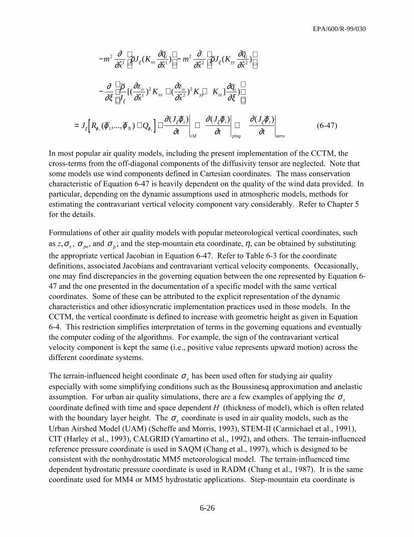
The generalized governing conservation equation for trace species, written in the Reynolds fluxform, is given in Equation 6-18. The same equation in eddy-diffusion form, in which thecomponents of the eddy diffusivity tensor are represented in terms of those in Cartesiancoordinates, is given below:

∂∂

ϕϕ ∂ ϕ

∂ξξ ξξ

ξξ

tJ m

J

m

J vi

i i( ) ˆ ˆ ( ˆ )+ ∇ •

+22

3

V

EPA/600/R-99/030

6-26

−

−

mx

J Kq

xm

xJ K

q

xxxi

yyi2

1 12

2 2

∂∂

ρ ∂∂

∂∂

ρ ∂∂ξ ξˆ

(ˆ

)ˆ

(ˆ

)

− + +

∂∂ξ

ρ ∂∂

∂∂

∂∂ξξJ

z

xK

z

xK K

qsfc sfc

xx yy zzi[(

ˆ) (

ˆ) ] )1

22

2

= +[ ] + + +J R QJ

t

J

t

J

ti iNi

cld

i

ping

i

aero

ξ ϕ ϕξ ξ ξϕ ϕ

∂ ϕ∂

∂ ϕ∂

∂ ϕ∂

( ,..., )( ) ( ) ( )

1 (6-47)

In most popular air quality models, including the present implementation of the CCTM, thecross-terms from the off-diagonal components of the diffusivity tensor are neglected. Note thatsome models use wind components defined in Cartesian coordinates. The mass conservationcharacteristic of Equation 6-47 is heavily dependent on the quality of the wind data provided. Inparticular, depending on the dynamic assumptions used in atmospheric models, methods forestimating the contravariant vertical velocity component vary considerably. Refer to Chapter 5for the details.

Formulations of other air quality models with popular meteorological vertical coordinates, suchas z,σ z , σ po, and σ p̃ ; and the step-mountain eta coordinate, η, can be obtained by substituting

the appropriate vertical Jacobian in Equation 6-47. Refer to Table 6-3 for the coordinatedefinitions, associated Jacobians and contravariant vertical velocity components. Occasionally,one may find discrepancies in the governing equation between the one represented by Equation 6-47 and the one presented in the documentation of a specific model with the same verticalcoordinates. Some of these can be attributed to the explicit representation of the dynamiccharacteristics and other idiosyncratic implementation practices used in those models. In theCCTM, the vertical coordinate is defined to increase with geometric height as given in Equation6-4. This restriction simplifies interpretation of terms in the governing equations and eventuallythe computer coding of the algorithms. For example, the sign of the contravariant verticalvelocity component is kept the same (i.e., positive value represents upward motion) across thedifferent coordinate systems.

The terrain-influenced height coordinate σ z has been used often for studying air qualityespecially with some simplifying conditions such as the Boussinesq approximation and anelasticassumption. For urban air quality simulations, there are a few examples of applying the σ z

coordinate defined with time and space dependent H (thickness of model), which is often relatedwith the boundary layer height. The σ z coordinate is used in air quality models, such as theUrban Airshed Model (UAM) (Scheffe and Morris, 1993), STEM-II (Carmichael et al., 1991),CIT (Harley et al., 1993), CALGRID (Yamartino et al., 1992), and others. The terrain-influencedreference pressure coordinate is used in SAQM (Chang et al., 1997), which is designed to beconsistent with the nonhydrostatic MM5 meteorological model. The terrain-influenced timedependent hydrostatic pressure coordinate is used in RADM (Chang et al., 1987). It is the samecoordinate used for MM4 or MM5 hydrostatic applications. Step-mountain eta coordinate is

EPA/600/R-99/030

6-27

used for NCEPÕs Eta meteorological model (Black, 1994, and Mesinger et al., 1988), but nooperational air quality model using the eta coordinate is available.

Table 6-3. Vertical Coordinates and Associated Characteristics

CMAQCoordinate

x̂3 = ξ

Definition ContravariantVerticalVelocity

v̂3

VerticalJacobian

Jξ

Remarks

Z w = dz

dt1 Geometric height

σz σ zsfc

sfc

Hz z

H z=

−−

d

dtzσ H z

Hsfc− H is the thickness of

model and σ z is thescaled height

σz σ zsfc

sfc

z z

H z=

−−

d

dtzσ H zsfc− Nondimensional height,

terrain-influenced

1 − σ poσ po

o T

os T

p p

p p= −

−−

d

dtpoσ p p

gos T

o

−ρ

Nondimensionalreference pressure

1 − σ p̃ σ ˜

˜˜p

T

s T

p p

p p= −

−−

d

dtpσ ˜ ˜

˜p p

gs T−ρ

Nondimensionalgeostrophic pressure

1−η η π ππ π

η= −−

T

s Tsfc

− d

dt

η π πρ η

s T

sfcg

−˜

Step-mountain ETA

ηsfco sfc T

o T

p z p

p p=

−−

( )

( )0

6.4 Nesting Techniques

The nested grid CTM is needed to provide the required high resolution simulations. At present,Models-3 CMAQ allows only static grid nesting. In static grid nesting, finer grids (FGs) areplaced (i.e., nested) inside coarser grids (CGs). The resolution and the extent of each grid aredetermined a priori and remain fixed throughout the CTM simulation. Static grid nestingconserves mass and preserves transport characteristics at the interfaces of grids with differentresolutions (Odman et al., 1995). It allows for effective interaction between different scales withefficient use of computing resources. On the other hand, the nest domain is redefined during asimulation with the dynamic nesting. Both static and dynamic nesting techniques allow one-wayor two-way exchange of information among FGs and the CG and periodically by independentlysimulating CTMs at each grid (coarse or nested) with its own time step. The dynamic nestingprocedure is not implemented in the CMAQ system.

In one-way nesting, the primary concern is the mass conservation at the grid interface whereboundary conditions are input to the FG using the CG solution. The advective flux at the inflow

EPA/600/R-99/030

6-28

boundaries of the FG is the flux as determined by the CG solution that passes through thisinterface. We also allow for time variation of the flux during the CG time step. This isperformed by computing the departure point of the last particle passing through the interface foreach FG time step. In the Lagrangian description, the mass crossing the interface is equal to thespatial integral of the concentration distribution between the departure point and the interface.Most flux-conserving advection schemes use the same Lagrangian concept to calculate the masstransfer between grid cells (e.g., Bott, 1989). During each FG time step, we meter into the FGthe exact amount of mass that would have crossed the interface on the CG (Byun et al., 1996).

In two-way nesting, the concentrations are updated in each CG cell by averaging theconcentrations of all the FG cells overlapping with the CG cell. Special care is required to assurestrict mass conservation at the grid interface. The mass of some species (e.g., radicals) may nolonger be conserved because, when advancing the FG solution, we perform nonlinear chemicaltransformations in addition to transport. However, the mass of the basic chemical elements suchas sulfur, nitrogen, and carbon must be conserved. The FG solution is used to compute the fluxof each element at the grid interface. When conservation principles are applied to the gridinterface, as described above, the CG concentrations near the interface must be corrected (whenthe Courant stability limit is applied, only the first row of CG cells immediately outside theinterface need correction). This is done by renormalizing the concentration of each species basedon the assumption that the ratio of the species mass to element mass will remain the same beforeand after the correction. This method is similar to the renormalization procedure used to makeslightly non-conservative chemical solvers strictly conservative. Alapaty et al. (1998) comparesdifferent spatial interpolation schemes used for the two-way nesting.

INPU

T

FEED

BAC

K

INPU

T

INPU

T

∆t

∆T

∆t ∆t

cCG

cFG

Figure 6-5. Static Grid Nesting Used in CMAQ System

The CCTM provides a static nesting (see Figure 6-5) capability while maintaining a high level ofmodularity by separately processing object codes for different grid domains and by enforcing theprotocol that each module reads its required input data independently from others. The scheme

EPA/600/R-99/030

6-29

is also applicable for multiple and multi-level grid nesting. Multi-level nesting is a naturalextension of the single static grid nesting. Figure 6-6 presents a schema for multi-level nesting,where three-levels are illustrated. The feedback processes update coarser grid concentrations ateach synchronization time steps of the nest grids. The information about the grid iscommunicated to each process module through a set of FORTRAN include files specific to eachgrid domain during compilation time. This allows use of the same process modules for differentgrids. Customizing a nested model is as simple as preparing include files with grid dimensions foreach grid and a driver with the appropriate process calling sequence.

As seen in Figure 6-6, the only difference between the one-way and two-way nesting is whetherconcentrations in coarser grid simulations are updated with the finer grid simulations through thefeedback processors or not. Depending on the computer hardware and software configurations,one could build a nested CTM model with one executable collectively simulating all the FGs andCG, or with independent CTM executables for different grids that run simultaneously onmultiple CPUs accessing common data through appropriate I/O API. The latter approach relieson the cooperating processors concept in a UNIX environment. As mentioned before, thecurrent CMAQ version lacks a feedback module, which is necessary for the two-way nesting.

cGridDriver

fGrid_1Driver

BCProc

FeedbackProc

fGrid_2Driver

BCProc

FeedbackProc

cGridJ file

cGridIC file

cGridBC file

cGridEmis

cGridMet Coarse_Conc

fGrid_1J file

fGrid_1IC file

fGrid_1Emis

fGrid_1Met fGrid_1_Conc

fGrid_2

J file

fGrid_2

IC file

fGrid_2Emis

fGrid_2Met fGrid_2_Conc

∆t_sync_cGrid

∆t_Sync_fGrid1

interpolateconc

UpdateCoarse

interpolateConc

UpdatefGrid_1

LegendcGrid: coarse grid domainfGrid: f ine grid domainEmis: emissions fileMet: meteoro logy filesJ: photo lysis rat eIC: initial condit ionsBC: boundary condit ionsConc: concentr ati onSync: synchronizat ionProc: processor

Figure 6-6. Schematics for Multi-level Nesting (three levels illustrated)

EPA/600/R-99/030

6-30

6.5 Summary

The CMAQ system achieves multi-pollutant and multiscale capabilities by combining severaldistinct modeling techniques. The generalized governing conservation equations of the CCTMallow transformation among various vertical coordinates (e.g., terrain-influenced geometric height,or pressure) and transformation among various horizontal coordinates, especially mapprojections (e.g., rectangular, Mercator, Lambert, and polar stereographic) by simple changes in afew scaling parameters defining the boundary domain, map origin, and orientation. Therefore,CMAQ can be configured to match the dynamic characteristics of the preprocessormeteorological models. The CMAQ system uses a nesting technique and a plume-in-gridapproach to handle small scale air quality problems and subgrid scale plume dispersion andchemical reactions, respectively. The multi-pollutant capability is provided by a generalizedmechanism reader and generalized chemistry solvers, linked cloud mixing and aqueous reactionprocesses, and aerosol modules. The CCTM code uses a modular structure that allows for thecontinuing improvement of the science and addition of new capabilities in a unified fashion. Itprovides a natural disciplinary distinction among different science processes through whichdevelopments in specific research areas can be readily incorporated.

As mentioned above, there remain a few implementation tasks, such as development of feed-backmodules for two-way nesting and adaptation of anholonomic coordinates (e.g., latitude-longitude), which will provide additional functionalities in CCTM.

6.6 References

Alapaty, K., R. Mathur, and T. Odman, 1998: Intercomparison of spatial interpolation schemesfor use in nested grid models. Mon. Wea. Rev. 126, 243-249.

Binkowski, F. and U. Shankar, 1995: The regional particulate model, Part I: Model descriptionand preliminary results. J. Geophys. Res., 100: 26191-26209.

Black, T., 1994: The new NMC mesoscale Eta model: Description and forecast examples. Wea.Forecasting, 9, 265-278.

Bott, A., 1989: A positive definite advection scheme obtained by nonlinear renormalization ofthe advective fluxes. Mon. Wea. Rev. 117, 1006-1015.

Byun D. W. , A. Hanna, C. J. Coats, and D. Hwang, 1995: Models-3 Air Quality ModelPrototype Science and Computational Concept Development. Trans. TR-24 RegionalPhotochemical Measurement and Modeling Studies, 8-12 November 1993, San Diego, CA, Air &Waste Management Association. Pittsburgh, PA., 197-212.

Byun, D.W., D. Dabdub, S. Fine, A. F. Hanna, R. Mathur, M. T. Odman, A. Russell, E. J.Segall, J. H. Seinfeld, P. Steenkiste, and J. Young, 1996: Emerging Air Quality ModelingTechnologies for High Performance Computing and Communication Environments, Air PollutionModeling and Its Application XI, ed. S.E. Gryning and F. Schiermeier, 491-502.

EPA/600/R-99/030

6-31

Byun, D.W., J. Young., G. Gipson., J. Godowitch., F. Binkowsk, S. Roselle, B. Benjey, J. Pleim,J. Ching., J. Novak, C. Coats, T. Odman, A. Hanna, K. Alapaty, R. Mathur, J. McHenry, U.Shankar, S. Fine, A. Xiu, and C. Jang, 1998: Description of the Models-3 Community MultiscaleAir Quality (CMAQ) model. Proceedings of the American Meteorological Society 78th AnnualMeeting, Phoenix, AZ, Jan. 11-16, 1998. 264-268.

Byun, D. W., 1999: Dynamically consistent formulations in meteorological and air qualitymodels for multi-scale atmospheric applications: II.ÊMass conservation issues. J. Atmos. Sci., (inprint).

Carmichael, G.R., L.K. Peters, and R.D. Saylor, 1991: The STEM-II regional scale aciddeposition and photochemical oxidant model-I. An overview of model development andapplications. Atmos. Environ. 25, 2077-2090.

Chang, J.S., R.A. Brost, I.S.A. Isaksen, S. Madronich, P. Middleton, W.R. Stockwell, and C.J.Walcek, 1987: A three-dimensional Eulerian acid deposition model: Physical concepts andformulation, J. of Geophys. Res., 92, 14,681-700.

Chang J. S., S. Jin, Y. Li, M. Beauharnois, C.-H. Lu, H.-C. Huang, S. Tanrikulu, and J. DaMassa,1997: The SARMAP air quality model. Final Report, SJVAQS/AUSPEX Regional ModelingAdaptation Project, 53 pp. [Available from California Air Resources Board, 2020 L Street,Sacramento, California 95814.]

Coats, C.J., cited 1996: The EDSS/Models-3 I/O Applications Programming Interface. MCNCEnvironmental Programs, Research Triangle Park, NC. [Available on-line fromhttp://www.iceis.mcnc.org/EDSS/ioapi/H.AA.html.]

Harley, R.A., A.G. Russell, G.J. McRae, G.R. Cass, and J.H. Seinfeld. 1993: Photochemicalmodeling of the Southern California air quality study. Envir. Sci. Technol. 27, 378-388.

Jacobson, M.Z. and R.P. Turco, 1994: SMVGEAR: A sparse-matrix vectorized Gear code foratmospheric models. Atmos. Environ. 20, 3369-3385.

Mesinger, F., Z. I. Janjic, S. Nickovic, D. Gavrilov, and D. G. Deaven, 1988: The step-mountaincoordinate: model description and performance for cases of Alpine lee cyclogenesis and for a caseof Appalachian redevelopment. Mon. Wea. Rev., 116, 1493-1518.

Odman, M.T., R. Mathur, K. Alapaty, R.K. Srivastava, D.S. McRae, and R.J. Yamartino, 1995:Nested and adaptive grids for multiscale air quality modeling. U.S. EPA Workshop on NextGeneration Models Computational Algorithms (NGEMCOM), Bay City, MI, June 1995.

Seaman, N. L., D. R. Stauffer, and A. M. Lario-Gibbs, 1995: A multiscale four-dimensional dataassimilation system applied in the San Joaquin Valley during SARMAP. Part I: Modeling designand basic performance characteristics. J. Appl. Meteor., 34, 1739-1761.

EPA/600/R-99/030

6-32

Seinfeld, J.H., 1986: Atmospheric Chemistry and Physics of Air Pollution. Wiley-Interscience,New York.

Scheffe, R. D., and R. E. Morris, 1993: A review of the development and application of theUrban Airshed Model. Atmos. Environ., 27B, 23-39.

Srivastava, R.K., D.S. McRae, M.T. Odman, 1995: Governing Equations of AtmosphericDiffusion. Technical Report, MCNC [Available from MCNC-North Carolina SupercomputingCenter, P.O. Box 12889, 3021 Cornwallis Rd. Research Triangle Park, NC 27709-2889.]

Schwartz, E. S. and P. Warneck, 1995: Units for use in atmospheric chemistry. Pure & Appl.Chem. 67, Nos 8/9, 1377-1406.

Toon, O.B., R.P. Turco, D. Westphal, R. Malone, and M.S. Liu, 1988: A multidimensionalmodel for aerosols: Description of computational analogs. J. Atmos. Sci., 45, 2123-2143.

Venkatram, A., 1993: The parameterization of the vertical dispersion of a scalar in theatmospheric boundary layer. Atmos. Environ. 27A, 1963-1966.

Yamartino, R.J., J.S. Scire, G.R. Carmichael, and Y.S. Chang, 1992: The CALGRID mesoscalephotochemical grid model - Part I. Model formulation, Atmos. Environ. 26A, 1493-1512.

Young, J.O., E. Sills, D. Jorge, 1993: Optimization of the Regional Oxidant Model for the Cray Y-MP, EPA/600/R-94/065. [Available from U.S. Environmental Protection Agency, ResearchTriangle Park, NC 27711.]

This chapter is taken from Science Algorithms of the EPA Models-3 CommunityMultiscale Air Quality (CMAQ) Modeling System, edited by D. W. Byun and J. K. S.Ching, 1999.

EPA/600/R-99/030

6-33

Appendix 6A. Concentration Units Used for Air Quality Studies

As we have seen above, many different concentration units are used for air quality studies. Inthis section we summarize the relations among the concentration units and their conversionfactors from one unit to another. For Models-3/CMAQ system we follow the InternationalSystem of Units (Syst�me International, SI) as a framework for units in the formulations. Thefundamental assumption used here is that air and trace gases follow the ideal gas law, i.e.,

pV R Tg= ν , (6A-1)

where Rg is the universal gas constant = 8.314510 [ J mol K/( )• ],

ν is molar number,V is volume of the gas [m3 ],p is pressure [Pa], andT is temperature [K].

There are many different ways to express the amount of substance in the atmosphere. Weintroduce most popular quantities and transformation relations among them are presented below.

Number Density, n

One way to express trace gas quantities is to count number of molecules in the unit volume. Forexample, number of molecules of air in the unit volume, nair , is expressed as:

nN

Vairair A= ν

(6A-2)

where νair is number of moles of air,

NA is the AvogadroÕs number = 6 0221367 1023. × , andSimilarly, number of molecules of trace gas per volume, i.e., number density of species ni, isdefined as:

nN

V

N

R T p

p

k Tii A i A

i g i

i

B

= = =ν νν /

[molecules m−3 ] (6A-3)

where ν i is number of moles of trace gas i in a given volume, and

k R NB g A= / is BolzmannÕs constant

pi is the partial pressure of species i.

Molar Density, ci

The number of moles of air (cair) and trace gas (ci) normalized for a unit volume of air are simplydefined as:

EPA/600/R-99/030

6-34

cVairair= ν

(6A-4a)

cVi

i= ν (6A-4b)

with the unit [ mole m −3]. Because the SI unit for the amount of substance is mol, this quantitycan be used conveniently for expressing chemical relationships.

Partial Pressure, pi

Although not used widely in atmospheric chemistry, the partial pressure has been playing animportant role specifying thermodynamic properties of the atmosphere, especially for watervapor in the air. The DaltonÕs law states that the total pressure exerted by a mixture of gases isequal to the sum of the partial pressure exerted by each constituent at the given temperature andvolume. Because we assume that each trace gas follows the ideal gas law, the partial pressurecan be used to express the trace gas quantity. The partial pressure of atmospheric constituentgas is related to the number of moles per volume as:

pR T

Vc R Ti

i gi g= =

ν(6A-5)

and the standard SI unit for the partial pressure is Pascal [Pa].

Molar Mixing Ratio, mi

Often, the molar mixing ratio is used as a synonym for the volume mixing ratio, or the molefraction of a substance in air. Basically it is a unitless quantity. However, it is customary toidentify in terms of molar unit as [ mole mole/ ]. Because the volume occupied by a mole of idealgas at given pressure is the same regardless of the constituent, the mole fraction is essentiallyequal to the volume fraction. However, mole fraction is preferred because it does not require theimplicit assumption of the ideality of the gases, and more importantly because it is applicablealso to condensed-phase species (Schwartz and Warneck, 1995). For a given volume, the volumemixing ratio of a trace species is expressed in terms of concentration units defined above as:

mc

c c

p

pii

air i

i

air i

i=+

=+

=νν ν

, (6A-6)

where p is the total pressure.

Because ν νi air<< for trace gases, Equation 6A-6 can be approximated as:

mc

c

p

pii

air

i

air

i

air

≈ = =νν

EPA/600/R-99/030

6-35

When dealing with trace gases in the real atmosphere, the contribution of moisture can be used inthe definition of mixing ratio. Therefore, pair represents total pressure of the atmosphere which

includes vapor pressure of water while the contribution of other trace gases are neglected.Because the variation caused by the moisture can amount to several percent, some researchersprefer to use dry air when expressing trace gas mixing ratios. However, in the Models-3/CMAQsystem, we use the trace gas mixing ratio with respect to the moist air because we rely on thecontinuity equation for the total air density to represent atmospheric mass conservation.

Mass Mixing Ratio, qi

Mass mixing ratio is used often for describing transport process and is simply related with thevolume mixing ratio as:

q mM

Mi ii

air

= (6A-7)

Density, ϕ i

Concentrations of substances in air can be expressed in terms of amount of substance mass pervolume of air, i.e. density. Density is a most popular unit for dynamic representation ofatmospheric concentration because it is the operating units of the mass continuity equation.Density can be expressed in terms of other concentration units as:

ϕ νi

i ii i

i

airair i

M

Vc M

c

cc M= = =

≈ =( )( )mM

Mc M qi

i

airair air i airρ (6A-8)

Table 6A-1 provides cross-reference relationships among the concentration variables described.However, the individual process science area prefers to use certain specific units of decimalmultiples of the SI unit suggested. We included the conversion factors among the concentrationvariables actually implemented in science process modules. Because it is convenient to expressthe conversion factors in terms of the dry air quantities, the virtual temperature is used in Table6A-1.

EPA/600/R-99/030

6-36

nu

mbe

rde

nsi

ty,N

i

[mol

ecu

les/

m3 ]m

ola

rde

nsi

ty,c

i

[mo

l/m

3 ]p

artia

lpre

ssur

e,pi

[Pas

cal]

mo

lar

mix

ing

ratio

,m

i[p

pm

V]m

ass

mix

ing

ratio

,q i

[pp

m]

den

sity

,ϕi[µ

g/m

3 ]

nu

mb

erde

nsi

ty,

Ni

[mo

lecu

les/

m3 ]

1N

i=

(NA)c

iN

i=

(kBT

)−1p i

Ni=

10−3

•N

A

ρ air

Ma

ir

m

iN

i=

10−3

•N A

ρ air

Mi

q

iN

i=1

0−6•

NA

Mi

ϕ

i

mo

lar

dens

ity,c

i

[mo

l/m

3 ]c i

=(N

A)−1

Ni

1c i

=(R

gT

)−1p i

c i=

10−3

•ρ air

Ma

ir

m

ic i

=1

0−3•

ρ air

Mi

q

ic i

=10

−6•

Mi

()−1

ϕ i

par

tialp

ress

ure

,p i

[Pas

cal]

p i=

k BT

()N

ip i

=R

gT

()c

i1

p i=

10−6

•(p)

mi

p i=1

0−6

•M

air

Mi

p

qi

p i=

10−6

•R

gT Mi

ϕ

i

mo

lar

mix

ing

ratio

,mi[p

pm

V]m

i=

103

•M

air

ρ airN

A

N

im

i=

103•

Ma

ir

ρ air

c

im

i=

106

•(p)

−1p i

1m

i=

Mair

Mi

q

im

i=

10−3

•M

air

ρ airM

i

ϕ

i

mas

sm

ixin

gra

tio,q

i[p

pm

]q i

=1

03•

Mi

NAρ air

N

iq i

=10

3•

Mi

ρ air

c

iq i

=1

06•

Mi

pM

air

p

iq i

=M

i

Ma

ir

m

i1

q i=

10−3

•ρ a

ir(

)−1ϕ i

den

sity

,ϕi

[µg

/m3 ]

ϕi

=1

06•

Mi

NA

N

iϕ

i=

106

•M

i(

)ci

ϕ i=1

06•

Mi

RgT

p iϕ i

=103

•ρ a

irM

i

Mair

m

iϕ

i=

103

•ρ a

ir(

)qi

1

Ta

ble

6A

.1.

Co

nve

rsio

n fo

rmu

la a

mo

ng

va

riou

s tr

ace

ga

s co

nce

ntr

atio

n u

nits

use

d in

the

CM

AQ

sys

tem

No

te: V

alu

es

for

the

Avo

ga

dro

’s c

on

sta

nt (

NA)

) is

6.0

22

13

67

x10

23

[nu

mb

er/

mo

l], th

e u

niv

ers

al g

as

con

sta

nt (

Rg)

is 8

.31

45

10

[J/m

ol-K

], a

nd

the

Bo

ltzm

an

n’s

con

sta

nt (k

B)

is d

efin

ed

with

Rg

/ N

A. M

ola

r m

ixin

g r

atio

is e

qu

iva

len

t to

vo

lum

e m

ixin

g r

atio

an

d th

eir

un

its [p

pm

V],

[pp

b],

an

d [p

pt]

are

sh

ort

ha

nd

no

tatio

ns

for

[ ], [

], a

nd

[ ],

resp

ect

ive

ly.

Th

e u

nit

for

ma

ss m

ixin

g r

atio

, [p

pm

], is

a s

ho

rt h

an

d fo

r [ ]

. B

oth

a

nd

m

ay

rep

rese

nt

valu

es

for

dry

air

or

mo

istu

re a

ir d

ep

en

din

go

n a

pp

lica

tion

s. H

ow

eve

r, in

on

e p

roce

ssin

g s

yste

m, t

he

ir u

sag

e s

ho

uld

be

co

nsi

ste

nt.

a

nd

(m

ole

cula

r w

eig

ht o

f sp

eci

es

i) a

re in

[g m

ol-1]

an

d

is in

[kg

m-3

].