The governing equations

PART II

The governing equations

Equations// [email protected] 43/374

1 The turbulence fact : Definition, observations and universal features ofturbulence

2 The governing equations

3 Statistical description of turbulence

4 Turbulence modeling

5 Turbulent wall bounded flows

6 Homogeneous Isotropic Turbulence

7 Homogeneous Shear Flows

8 Results based on the equations of the dynamics in fully developedturbulence


2 The governing equationsNavier-Stokes EquationsVorticityPressure in incompressible flowsNS equations and SymmetriesDimensionless numbersNon viscous invariantsValidityCharacteristics of turbulent flowsHomogeneity and isotropyCanonical turbulent flowsExercises


The Navier Stokes equations

Leonardo da Vinci, Sul Volo degli Ucceli, 1505A bird flies according to mathematical principles.

Equations/NS equations/ [email protected] 46/374


Mass conservation : local and conservative form

@⇢

@t+

@⇢uj

@xj

= 0 , 8 (x, t) (1)

x space variablet time⇢(x, t) densityu(x, t) velocity field



Momentum equation : HistoryLeonardo da Vinci (1452 � 1519)Isaac Newton :

m ⇥ � =X

F

Leonhard Euler :

Equation for a fluid particle

Claude Navier in 1823 :

Viscous term


The Navier Stokes equations (Newtonian fluids)Momentum equation : component form (non conservative)

⇢@ui

@t+ ⇢uj

@ui

@xj

= ⇢fi +@�ij

@xj

(2)

f : mass forces density (e.g. gravity g)� : stress tensor, second-order tensor

�ij ⌘ �p�ij + 2µSij + �@u`

@x`

�ij ,

where � and µ are the Lamé coefficients.

S : deformation rate tensor, second order. Sij ⌘ 12

⇣@ui@xj

+ @uj

@xi

⌘

�ij : Kronecker symbolVolume viscosity : K ⌘ � + 2

3µ, K = 0 for monoatomic gas.Usual approximation : � = � 2

3µ for air.Einstein summation convention



Momentum equation : component form

⇢Dui

Dt= � @p

@xi

+ µ

@2ui

@x2k

+1

3

@

@xi

@uk

@xk

�+ Fi (i = 1, 3) (3)

with the material derivative defined as

Dui

Dt⌘ @ui

@t+ uj

@ui

@xj

⇢ densityµ dynamic viscosityp pressure fieldu velocity field



Momentum equation : with vectorial operators

⇢Du

Dt= ⇢f � rp + r · (2µS) + r(�r · u) (4)

withDu

Dt=

@u

@t+ (r ⇥ u) ⇥ u + ru2

2

f : mass forces density ( e.g. gravity g)S : second order deformation rate tensor

Sij ⌘ 1

2

✓@ui

@xj

+@uj

@xi

◆



Thermodynamicsp = R⇢T : Ideal gas lawe = CvT : Internal energy ; Cv heat capacity at constant volumeh = CpT : Enthalpy ; Cp heat capacity at constant pressureR = Cp � Cv : Ideal gas constant� = Cp/Cv : Specific heat ratioAir : Diatomic gases around 78% nitrogen (N2) and 21% oxygen (O2).At standard conditions ⇠ ideal gas =) � ⇠ 1.4

First law for energy : E = ⇢V (e + u2)

�E = �Q � �W i.e. Heat � Work

Gibbs relation for entropy

Tds

dt=

de

dt+ P

d

dt

✓1

⇢

◆



Internal energy equation : Non-conservative form

@e

@t+ uj

@e

@xj

= �(� � 1)e@uk

@xk

+1

⇢�ijSij +

⇢

@2T

@x2k

(5)

e(x, t) internal energy

S : deformation rate tensor, tensor of second order. Sij ⌘ 12

⇣@ui@xj

+ @uj

@xi

⌘

� : viscous strain tensor, second-order

�ij = 2µSij + �@u`

@x`

�ij

where � is the second coefficient of viscosity.Stokes’ assumption for convenience : � ⌘ � 2

3µ.



Internal energy equation : Conservative form

@⇢e

@t+

@⇢uje

@xj

= �p@uk

@xk

+ �ijSij +@

@xk

✓

@T

@xk

◆(6)

⇢uje : Internal energy flux due to advection

�p@uk

@xk

: Net work of pressure force

�ijSij : Net work of viscous force@

@xk

✓

@T

@xk

◆: Net heat transfer



3D Incompressible flowsHyp : ⇢ constant

Pb : 4 equations, 4 unknowns (ui, p), 4 independent variables (xi, t)8>><

>>:

@ui

@xi

= 0

⇢@ui

@t+ ⇢uj

@ui

@xj

= � @p

@xi

+ µ@2ui

@x2j

+ Fi (i = 1, 3)(7)

Non linear, coupled, partial differential equations !



Viscosity

µ : dynamic viscosity [M ][L]�1[T ]�1

⌫ = µ/⇢ : kinematic viscosity [L]2[T ]�1

Typical values of µ for air and water

Air at 300 K, 1 atm : µ ⇠ 18.46 ⇥ 10�6(Ns)m�2

Air at 400 K, 1 atm : µ ⇠ 23.01 ⇥ 10�6(Ns)m�2

Liquid water at 300 K, 1 atm, µ ⇠ 855 ⇥ 10�6(Ns)m�2

Liquid water at 400 K, 1 atm, µ ⇠ 217 ⇥ 10�6(Ns)m�2

Sutherland’s FormulaDynamic viscosity (Pa.s) of an ideal gas as a function of thetemperature

µ = µ0T0 + C

T + C

✓T

T0

◆3/2

C : Sutherland’s constant for the gaseous material


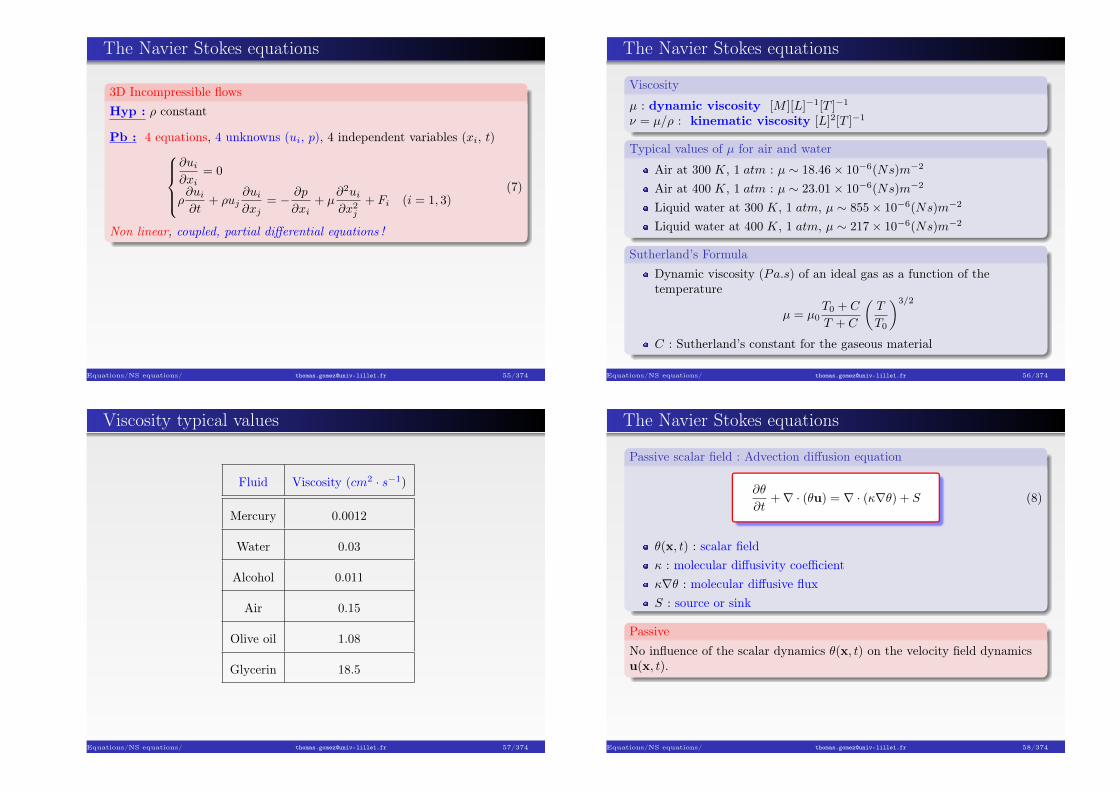
Viscosity typical values

Fluid Viscosity (cm2 · s�1)

Mercury 0.0012

Water 0.03

Alcohol 0.011

Air 0.15

Olive oil 1.08

Glycerin 18.5



Passive scalar field : Advection diffusion equation

@✓

@t+ r · (✓u) = r · (r✓) + S (8)

✓(x, t) : scalar field : molecular diffusivity coefficientr✓ : molecular diffusive fluxS : source or sink

PassiveNo influence of the scalar dynamics ✓(x, t) on the velocity field dynamicsu(x, t).


Passive scalar dynamics

Advection diffusion equation

@✓

@t+

@✓uj

@xj

=@

@xj

✓

@✓

@xj

◆

| {z }Diffusiveflux

+S (9)

Passive scalar field : ✓(x, t)

Temperature (small fluctuations)Polluant concentration


The Navier Stokes equations + Passive Scalar

3D Incompressible flowsHyp : ⇢ constant

Pb : 5 equations, 5 unknowns (ui, p, ✓), 4 independent variables (xi, t)8>>>>>><

>>>>>>:

@ui

@xi

= 0

⇢@ui

@t+ ⇢uj

@ui

@xj

= � @p

@xi

+ µ@2ui

@x2j

+ Fi (i = 1, 3)

@✓

@t+ uj

@✓

@xj

=@

@xj

✓

@✓

@xj

◆+ S

(10)


Exercice :Write the momentum equation under a conservative form


The Navier Stokes equations : Initial and Boudaryconditions

Geometry and physics of the flowPeriodic boxWall (slip / no slip)Pressure outletFlux (mass, momentum or energy)Dirichlet/Neumann. . .

=) Boundary conditions

Physics of the flow : Initial statePressure, Internal energy,Temperature, DensityVelocityPolluant concentration

=) Initial conditions


Scalar dynamics examples

Advection diffusion equation : case 1

1D flowUniform and constant velocity u1

Initial condition ✓0 at (x0, t0)

S = 0

No diffusivity

Advection diffusion equation : case 2

Same initial conditionNo convectionS = 0

Diffusivity


Vorticity dynamics

DefinitionVorticity :

!!! = r ⇥ u

Einstein notation :

!i = "ijk

@uk

@xj

= "ijk@juk

"ijk : Levi-Civita symbol, permutation symbol, antisymmetric symbol,or alternating symbol

PropertiesDivergenceless tensor : @j!j = 0

Pseudo-tensor : don’t satisfy the parity (or mirror) symmetry

Equations/Vorticity/ [email protected] 63/374

Vorticity dynamics in turbulents flows

Boundary layer


Vorticity dynamics in turbulent flows

Compressible turbulent flow in 3D periodic cubic box

Iso-value of the vorticityDNS of Compressible flowD. H. Porter, A. Pouquet,and P. R. Woodward


Vorticity dynamics

Incompressible turbulent flow in 3D cubic box


Vorticity dynamics in turbulent flows

EquationVorticity :

!!! = r ⇥ u =) r ⇥ (NS)

Vorticity equation :

@!i

@t+ uj

@!i

@xj

= !j

@ui

@xj

+ ⌫@2!i

@xk@xk

+ r ⇥ fi (i = 1, 3)

RemarksNo pressure termStretching increases vorticy intensity

ExerciseDerive the governing equation for the vorticity dynamics.Show that !j@jui = !jSij .


Pressure in incompressible flows

Non local quantity ! and non linear...

Equations/Pressure in incompressible flows/ [email protected] 68/374


Poisson problem



Filament of vorticity tracerAir bubbles =) minimum of pressure () �p � 1


NS equations and Symmetries

HypothesisUnboundeness of the space, or more strictly periodic boundary

conditions.Incompressible flow : @iui = 0.

Transformations acting on space-time functions

x �! x0 , t �! t0 , u(x, t) �! v(x0, t0)

Equations/Symmetries/ [email protected] 71/374


Symmetry group of the NS equationsSpace translation

(x, t) �! (x0 = x + r, t0 = t) , v(x0, t0) = u(x, t)

Time translation

(x, t) �! (x0 = x, t0 = t + ⌧) , v(x0, t0) = u(x, t)

Galilean transformation

(x, t) �! (x0 = x + u0t, t0 = t) , v(x0, t0) = u(x, t) + u0

ExerciseShow that NS equations are invariant under space and timetranslation.Show that NS equations are invariant under Galilean transformation.



Symmetry group of the NS equationsParity

(x, t) �! (x0 = �x, t0 = t) , v(x0, t0) = �u(x, t)

Rotation

A 2 SO(R3)(x, t) �! (x0 = Ax, t0 = �1�ht) , v(x0, t0) = Au(x, t)

ScalingCondition on h 2 R, ⌫ = 0 and h = �1, ⌫ 6= 0

(x, t) �! (x0 = �x, t0 = �1�ht) , v(x0, t0) = �hu(x, t)


Dimensionless numbers

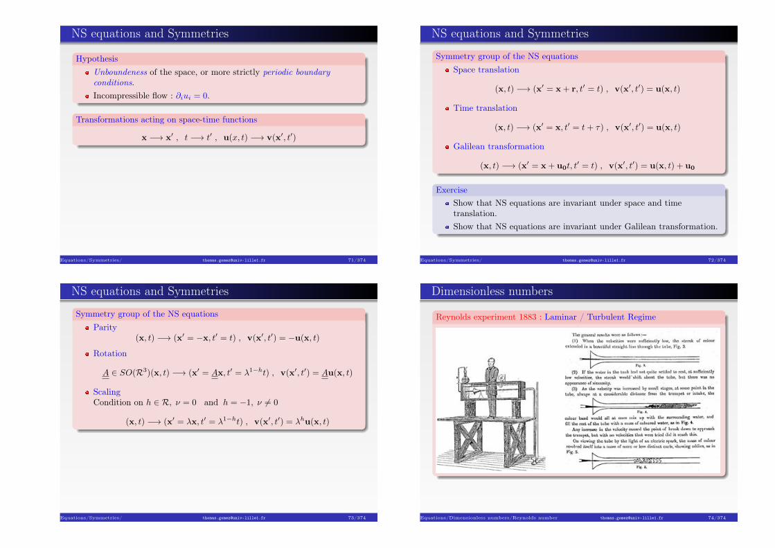
Reynolds experiment 1883 : Laminar / Turbulent Regime

Equations/Dimensionless numbers/Reynolds number [email protected] 74/374

Dimensionless numbers : Reynolds number Re

From dimensional analysis and similarity theory

Characteristic quantitiesU : Velocity scaleL : Length scaleµ : viscosity⇢ : density

⇢u · ru| {z }NL term

⇠ ⇢U2

Land µr2u| {z }

Viscous term

⇠ µU

L2

Reynolds number Re =⇢UL

µ⇠ Inertial effect

Viscous effect(11)


Dimensionless numbers

Reynolds number Re

Re ⌧ 1 Laminar flowsRe � 1 Turbulent flowsControl parameterRec : Critical Reynolds

Re =⇢UL

µ⇠ Inertial effect

Viscous effect

(12)


The Navier Stokes equations : Non-dimensionalized form

Incompressible flowsHyp : ⇢ constant, 4 equations, 4 unknowns (ui, p), 4 variables (xi, t)

8>><

>>:

@ui

@xi

= 0

⇢@ui

@t+ ⇢uj

@ui

@xj

= � @p

@xi

+1

Re

@2ui

@x2j

+ Fi (i = 1, 3)(13)


Re �! +1 =) Euler equations.Re �! +1 =) Turbulent fields !


Jets : Laminar �! Turbulent

�! �! �! �! �!

Reynolds number %


Typical Reynolds numbers

Flow Viscosity Velocity Lengthscale Reynolds number

(cm2 · s�1) m · s�1 m

Atmosphere 0.15 10 5 107

Water pipe 0.011 0.1 0.05 5.103


Dimensionless numbers : Strouhal number S

Characteristic quantitiesU : Velocity scaleL : Length scaleT : Time scale

@ui

@t|{z}Unsteady

⇠ U

Tand uj

@ui

@xj| {z }Advection

⇠ U2

L

Strouhal number S =L

UT=

Lf

U⇠ Unsteady

Advection(14)

Equations/Dimensionless numbers/Strouhal number [email protected] 80/374

Wakes : flows around a cylinder


Cont’d – Wakes : flow around a cylinder


Cont’d – Wakes : flow around a cylinder

Fixed cylinder


Dimensionless numbers : Prandtl number Pr

Characteristic quantities⌫ : Viscosity : Heat diffusionD : Mass diffusion

Prandtl number Pr =⌫

⇠ Momentum diffusion

Heat diffusion(15)

Schmidt number Sc =⌫

D⇠ Momentum diffusion

Mass diffusion(16)

Equations/Dimensionless numbers/Prandtl number [email protected] 84/374

Dimensionless numbers : Prandtl number Pr

Prandtl number Pr =⌫

⇠ Momentum diffusion

Heat diffusion

Typical values

PrHelium, Hydrogene, Azote 0.7

carbon dioxide 0.75Air 0.7

Water vapor 1.06Liquid water 7Engine oil 10400Mercury 0.025

Liquid sodium very smallSun 10�9

Equations/Dimensionless numbers/Prandtl number [email protected] 85/374

Non viscous invariants : ⌫ = 0

Physical quantitiesKinetic energy in 3D

E ⌘ 1

2

Z|u|2 dv

Helicity in 3D

H ⌘ 1

2

Z

V

u · !!! dv

Enstrophy in 2D

⌦ ⌘ 1

2

Z

V

!!!2 dv

Equations/Non viscous invariants/ [email protected] 86/374

Non viscous invariants

Conservation lawsConsidering any quantity h satisfying

@h

@t+ uj

@h

@xj

= g

The advection velocity is divergenceless

@uj

@xj

= 0

Then

8 V ,

Z

V

uj

@h

@xj

dv =

Z

S

(ujh)nj ds

⌘ 0 if u = 0 on S = @V .



Kinetic energyDefinition

E ⌘ 1

2

Z|u|2 dv

Governing equation

dE

dt=

Z

V

�r ·u

✓u2

2+

p

⇢

◆+ ⌫!!! ⇥ u

�

| {z }Flux term

dv � ⌫

Z

V

!!!2 dv

| {z }Dissipation

Then E is an invariant of the dynamics if ⌫ = 0 and u = 0 on S = @V .



Kinetic HelicityDefinition

H ⌘ 1

2

Z

V

u · !!! dv

Governing equation when u = 0 on S = @V .

dH

dt= �2⌫

Z

V

!!! · r ⇥ !!! dv

Then H is an invariant of the dynamics if ⌫ = 0.

Exercise

1 Write the flux term for the kinetic helicity equation.2 Show that the enstrophy ⌦ is a non viscous invariant of the 2D dynamics.


Non viscous 2D/3D invariants

Invariants


Validity of NS equations

In the wide senseMass conservationMomentumEnergy (1st Principle)2nd Principle

Validity

No mathematical proof of existence and unicity of solutions in 3D

Validity guaranteed today if flow properties do not vary at the scale of them.f.p, i.e. molecular scale.

Knudsen number :

Kn =m.f.p.

L,

L : characteristic length scale of the flow.

Equations/Validity/ [email protected] 91/374

Validity of NS equations (cont’d)

Knudsen numberKn < 10�2 : Continuous regime.10�2 < Kn < 10�1 : Sliding regime =) local anomalies near the walls.10�1 < Kn < 10 : Transitional regime =) Boltzmann equationsneeded.10 < Kn : Free molecular regime =) Molecular collisions negligable.

On earth

m.f.p.⇠ 10�7m and L ⇠ 10�3 =) Kn ⇠ 10�4.

At 11km, m.f.p.⇠ 3.10�7m

At 20km, m.f.p.⇠ 1.5 10�6m=) NS equations valid in 99% of case.

Equations/Validity/ [email protected] 92/374

Characteristics of turbulent flows

Irregularity in space and timecf. examples in section 1

Wind tunnelFrisch 1995

Equations/Characteristics of turbulent flows/ [email protected] 93/374


Diffusive characterExample : Heating of a room

A room of size L.Heater in the room.

No motion in the roomHeat equation =) molecular diffusion

@✓

@t+ uj

@✓

@xj

=@

@xj

✓

@✓

@xj

◆

| {z }Diffusiveflux

+ S (17)

: thermal conductivity.Conducting characteristic time :

Tc ⇠ L2/ .



Diffusive characterExample : Heating of a room

A room of size L.Heater in the room.

Turbulent motion in the roomHypothesis :

L : size of the largest turbulent structures L ⇠ 10 m.u : turbulent velocity scale u ⇠ 1 cm.s�1.Characteristic time :

Tt ⇠ L/u ⇠ 103s .

Exercise

1 Give an estimation of Tc and compare the both characteristic time Tt andTc. Conclusion ?



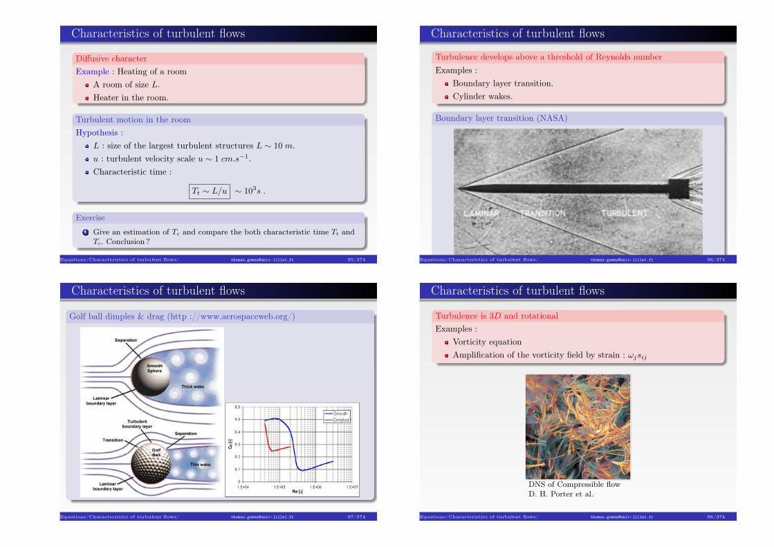
Turbulence develops above a threshold of Reynolds numberExamples :

Boundary layer transition.Cylinder wakes.

Boundary layer transition (NASA)



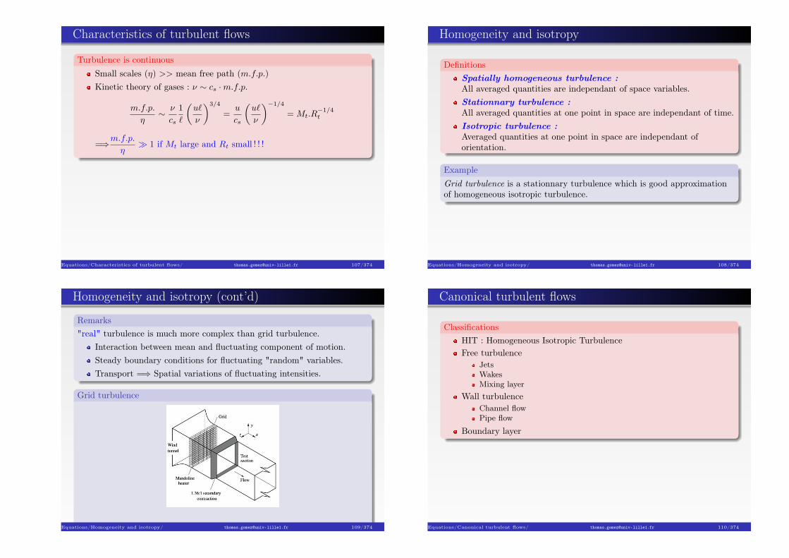
Golf ball dimples & drag (http ://www.aerospaceweb.org/)



Turbulence is 3D and rotationalExamples :

Vorticity equationAmplification of the vorticity field by strain : !jsij

DNS of Compressible flowD. H. Porter et al.



Turbulence is structured by a superposition of many vortices of differentcharacteristic scales interacting

Turbulence has a continuous spectrum of kinetic energy.Large range of active scales.



Kinetic energy spectrum



Turbulence is dissipativeExample

Friction in a boundary layer.Energy feeding of turbulence : c.f. Section on boundary layer

dynamics.



The largest scales are fixed by the characteristic size of the flowExamples

Boundary layer.Wake

Largest scale



The turbulence is non linearExample : 1D ideal flows (Burgers equation) or equivalently at largeReynolds number

@u

@t+ u

@u

@x= 0

=) Energy transfer from low to high frequencies

ExerciceConsidering the 1D ideal Burgers equation associated to an initialcondition under the form

u = u0 cos(kx) , for t = t0 ,

show that at small time an energy transfer from low to high frequenciesoccurs, i.e. from large to small scales.



The size of the smallest structures is fixed by the viscosity` : length scale of a structureu` : velocity scale of a structure

u@xu| {z }NL convective term

⇠ u2`

`and ⌫@2

xxu| {z }

diffusion

⇠ ⌫u`

`2

Re�1`

=⌫

u``⇠ diffusion

convection(18)

=) when ` & viscosity dominates and damps the turbulentstructures.=) small length scales () small time scales.=) statistical independance of small scales.



The size of the smallest structures is fixed by the viscosity (Kolmogorov41)

Hyp 1 : depend only on viscosity and rate of energy transfer fromthe large scales.

Hyp 2 : Equilibrium turbulence : Transfer rate = dissipation rate(no accumulation)Dimensional analysis : Energy 1

2u2i

and dissipation ⌫( @ui@xj

)2

=)(

" (m2 · s�3) dissipation rate,⌫ (m2 · s�1) kinematic viscosity.

Kolmogorov micro-scales :

⌘ =

✓⌫3

"

◆1/4

, u⌘ = (⌫")1/4 , ⌧⌘ =⇣⌫

"

⌘1/2.



The size of the smallest structures (cont’d)Non viscous estimation of "`

"` ⇠ u3`

`

Characteristic ratio :

⌘

`⇠

✓u``

⌫

◆�3/4

= R�3/4`

uL

u⌘

⇠ R1/4L

and⌧L

⌧⌘

⇠ R1/2L



Turbulence is continuousSmall scales (⌘) >> mean free path (m.f.p.)Kinetic theory of gases : ⌫ ⇠ cs · m.f.p.

m.f.p.

⌘⇠ ⌫

cs

1

`

✓u`

⌫

◆3/4

=u

cs

✓u`

⌫

◆�1/4

= Mt.R�1/4t

=)m.f.p.

⌘� 1 if Mt large and Rt small ! ! !


Homogeneity and isotropy

DefinitionsSpatially homogeneous turbulence :All averaged quantities are independant of space variables.Stationnary turbulence :All averaged quantities at one point in space are independant of time.Isotropic turbulence :Averaged quantities at one point in space are independant oforientation.

ExampleGrid turbulence is a stationnary turbulence which is good approximationof homogeneous isotropic turbulence.

Equations/Homogeneity and isotropy/ [email protected] 108/374

Homogeneity and isotropy (cont’d)

Remarks"real" turbulence is much more complex than grid turbulence.

Interaction between mean and fluctuating component of motion.Steady boundary conditions for fluctuating "random" variables.Transport =) Spatial variations of fluctuating intensities.

Grid turbulence

Wind tunnelFrisch 1995

Equations/Homogeneity and isotropy/ [email protected] 109/374

Canonical turbulent flows

ClassificationsHIT : Homogeneous Isotropic TurbulenceFree turbulence

JetsWakesMixing layer

Wall turbulenceChannel flowPipe flow

Boundary layer

Equations/Canonical turbulent flows/ [email protected] 110/374

Canonical turbulent flows (cont’d)

Similarity

Power of x for uc y1/2

Plane wake �1/2 1/2Axisym. wake �3/4 1/4Mixing layer � 1

Plane jet �1/2 1Axisym. jet �1 1Radial jet �1 1

Jet

Equations/Canonical turbulent flows/ [email protected] 111/374

Exercises

The characteristic scales of the turbulent dynamics

1. The small scalesWe assume that the small scale quantities of the turbulent flow can beexpressed only in terms of the dissipation rate by mass unit " (m2.s�3) andthe kinematic viscosity ⌫ (m2.s�1).

1 Using dimensional analysis, determine the characteristic velocity andtime scales, respectively denoted u⌘ and ⌧⌘ at the small length scale ⌘.These scales are called the micro-scales of the turbulent flows.

2 Write the Reynolds number based on these micro-scales and concludeabout the physical meaning of these scales.

Equations/Exercises/ [email protected] 112/374

Exercises


2. The large scales1 Let’s assume that the dynamics of the large scales can be characterized

by a velocity scale U and a length scale L. Using these bothcharacteristic scales, express the corresponding time ⌧L, so called theturnover time, characteristic of the kinetic energy transfer time. Thelength L is characteristic of the biggest eddies size of the flow.

2 Determine an expression for the kinetic energy transfer T through thescales from large to small scales.

3 Write the viscous characteristic time for the large scale and determinethe transfer rate T⌫ from large scales due to the viscous effects.

4 Compare the transfer terms T and T⌫ . What can we conclude whenRe � 1.


Exercises


3. Interscales relations1 Assuming the turbulence is steady, determine the transfer rate T and

T⌘ as function of ".2 Express the ratios L/⌘, ⌧L/⌧⌘ and U/u⌘ in term of the Reynolds

number Re = UL/⌫. Conclusions ?3 In order to describe the spatial scales of a turbulent 3D flow using a

numerical simulation, each space direction is discretized with a givennumber of points n. Determine the total number of points needed todescribe the 3D Flow in term of the Reynolds number.


Exercises

Dispersion law of a polluantRidchardson, Proc. Roy. Soc. London, 110, (1926).

Let’s consider two particles injected in a turbulent flow initially located ata distance d0 from each other. We assume that it exists a scale rangeL � ` � ⌘, so called the inertial range, in which the mean rate of kineticenergy dissipation " is assumed to be constant.

1 Express the kinetic energy dissipation rate "` at the scale ` in terms ofthe velocity and time characteristic scales, respectively denoted u`

and t`, then in terms of u` and ` only.2 Give an expression for u` in terms of "` and `. Assuming that "` is

constant through the scales, write a differential equation satisfied by `.3 Solve this equation and give a law for the time evolution of the

distance between two particles initially at the distance d0.


Exercises

Beltrami FlowsLet’s consider a flow defined by the following velocity field :

u =

8<

:

u1 = C sin ↵z + B cos ↵yu2 = A sin ↵x + C cos ↵zu3 = B sin ↵y + A cos ↵x

(19)

1 Show that this flow is incompressible.2 Show that the velocity field satisfies the Beltrami property, i.e.

!!! = �u

where � 2 IR. Give � as function of ↵.3 Write the non-linear terms of the Navier-Stokes equations written for

the vorticity. What can we conclude ?


Exercises

Atomic blastLet’s assume that, in an atomic explosion, a release of a significant amount ofenergy E occurs instantaneously within a small region (one may say, at a point).In the early stage, a strong spherical shock wave develops at the point ofdetonation.

1 Let’s assume that the radius R of the shock wave front, at an interval oftime t after the explosion only depends on the quantities E, t and on theinitial air density ⇢0. Using dimensional analysis, give an expression for R interms of E, t and ⇢0.

2 Then give an expression of E in terms of R, t and ⇢0.3 From a series of high speed photograph, Taylor has measured that the front

was at R = 125m at time t = 0.025s. Give the Taylor’s estimation of theenergy of the explosion. This was considered as top secret and caused ’muchembarrassment’ in American government circles. NA : ⇢0 = 1.3kg/m3.


Exercises

Atomic blast (Cont’d)

+ =)

Figure: First atomic bomb called Gadget at the top of a tower, July 15th 1945and its Fireball 25ms after an atomic explosion on the ground.


The governing equations

Documents

Transcript of The governing equations