Chapter 6

A QUANTITATIVE APPROACH TO

EVALUATING INTERNATIONAL

ENVIRONMENTAL REGIMES

RONALD B. MITCHELL University of Oregon

1. INTRODUCTION

To date, analysts of international environmental regimes have largely eschewed quantitative methods.1 Yet, applying statistical procedures to large sets of quantified data offers rich opportunities to address questions central to this research program. Quantitative analysis can shed light on questions that either cannot be or usually are not answered by qualitative methods while also allowing reexamination of questions already addressed by such methods. Careful modeling and analysis of appropriate data could identify which features of a regime are responsible for a regime’s success and which are superfluous, how much of a contribution regimes can make to resolving environmental problems, and the extent to which the effectiveness of a particular type of regime depends on factors such as the type of problem or international context. Thus, quantitative analysis offers a valuable complement to qualitative techniques in evaluating regime effects and effectiveness.

Consider some questions regarding regime effectiveness. Are sanctions always more effective at inducing behavioral change than rewards and, if not, under what conditions are rewards more effective?2 Are pollution problems, on average, more difficult or easier to resolve than wildlife preservation problems? Do demands for new behaviors generally work better or worse than bans on existing behavior?3 Such questions are difficult

121

A. Underdal and O.R. Young (eds.), Regime Consequences, 121–149.

© 2004 Kluwer Academic Publishers. Printed in the Netherlands.

122 R. B. MITCHELL

to answer convincingly with case studies of single regimes because most regimes do not employ both sanctions and rewards, address both pollution and wildlife problems, or ban some behaviors while requiring others. We certainly want to analyze those rare regimes that exhibit such variation, since they convincingly control many other variables. Yet, case studies face inherent problems of generalizability. Even commendable recent efforts to draw conclusions across multiple regimes, each analyzed by a different scholar, face difficulties in ensuring convincing comparability across regimes.4 The findings of carefully designed case studies often fit the case studied well but cannot be convincingly extended to many, and sometimes to any, other cases.5

Quantitative analysis involves the opposite trade-off, generating propositions that hold reasonably well across many cases but that cannot explain any particular case well.6 It can identify what “tends to happen” in regimes in general or in regimes of particular types. It can tell us whether the influence of regimes on behavior is generally larger or smaller than other influences. It can help “fill in the blanks” left by qualitative analysis, using patterns across regimes to clarify why certain types of regimes address certain types of problems better than others, or why regimes in one issue area work better than otherwise-similar regimes in a different issue area. Such comparisons across regimes can move us beyond case study insights that a particular type of regime can produce a desired outcome to the often more useful claim that such a design is likely to produce such an outcome in some other context, moving us from possibility to probability. Large-N comparisons allow us to refine claims of qualitative research, such as, evaluating the general claim that country capacity influences compliance by examining whether the lack of a particular capacity inhibits compliance with some types of regimes but not others.7 Quantitative techniques offer the promise of replacing claims that “this strategy worked in this historical case” with more convincing policy-relevant and contingent prescriptions of which strategy is likely to work best to address a given problem under given conditions. Although a variety of quantitative techniques could be used to investigate regime consequences, in this chapter I delineate one quantitative approach, that of using regression analysis on panel data.8

2. DEFINITIONS

Recent work on qualitative methodology in general and counterfactuals in particular reminds us that any attempt to make causal claims requires comparing at least two cases.9 Here I clarify some terms useful for discussing quantitative study design, generally avoiding the term “case”

A QUANTITATIVE APPROACH 123

because of its multiple, often widely divergent, meanings.10 Units of analysisare the entities or phenomena about which the researcher collects data.11

Units of analysis, often called cases, are a sample from a population or class of all conceptually-similar units that could have been studied. Variables are the dimensions, characteristics, or parameters of these units of analysis, with any variable having two or more possible values. Quantitative studies examine covariation between the values of two variables in a database in hopes of distinguishing underlying causal relationships among those variables in the world. Dependent variables (DVs) are those whose variation we seek to explain. Explanatory or independent variables (IVs) are those whose variation we look to as possible explanations of the variation in the DV, based on theoretical claims regarding their causal influence on that DV. Control variables (CVs) are IVs believed to influence the DV that are included in an analysis in order to separate their influence on the DV from that of the primary IV of interest. To avoid confusion, I distinguish between a unit of analysis and an observation. An observation is one set (or vector) of the observed values of all variables (IVs, CVs, and DV) for a given unit of analysis. These definitions allow us to speak of multiple observations of a single unit of analysis, as when we observe a regime (the unit of analysis) at several points in time. In a spreadsheet analogy, each column corresponds to a different variable (IV, CV, or DV); each row corresponds to a single observation; each cell contains the value of a given variable for a given observation; the first column contains a name (or other identifier) for each observation; and the dataset could contain rows corresponding to multiple observations from each unit of analysis as well as observations from multiple units of analysis. A quantitative study of regime consequences requires defining some potential consequent of regimes as a dependent variable, the presence or absence of a regime or some regime characteristic as the independent variable of interest, and some set of other factors predicted to affect the dependent variable as control variables. The analyst would then seek out regimes (units of analysis) that allow relatively comparable observations across these IVs, CVs, and DVs.

Given these definitions, qualitative research is best distinguished from quantitative research by the fact that the former examines relatively few units of analysis while the latter examines many. The benefit of a qualitative approach stems from the fact that the study of one or two units of analysis holds many variables constant across however many observations are analyzed (since many variables are constant across all observations of a given unit of analysis). This eliminates those variables as potential explanations of variation in the DV and thereby improves the ability to evaluate the influence on the DV of the remaining IVs that do vary. The benefit of a quantitative approach lies in capturing evidence from a sufficient

124 R. B. MITCHELL

number of different units of analysis that one can determine whether the influence of one or two IVs on the DV holds across a wide range of values for the many variables that are likely to vary across these units of analysis. Beyond this definitional distinction, in practice quantitative analysis usually examines not only more units of analysis but also more observations and more independent and control variables.

Finally, although recognizing the value of a broader definition, I use regime here to refer to the governance structures surrounding international conventions and treaties, including the norms, rules, principles, and decision-making procedures as well as the numerous actors who bring those components to life.12

3. MODELING FOR QUANTITATIVE ANALYSIS

OF REGIME EFFECTS

A long list of regimes now exists which case studies have shown to have been effective.13 As much of the literature and other chapters in the present volume clarify, regime effectiveness has multiple possible meanings.14 A quantitative approach has the advantage of addressing questions central to this literature while separating the identification of regime effects from the judgment of regime effectiveness. A regime’s effects are those changes in some DV of interest to the analyst that are best explained by the regime and cannot be explained by other variables. Indeed, most regimes have both intended and unintended, direct and indirect, and desirable and undesirable effects.15 Although effectiveness can be used as a synonym for direct and intended effects, more often a regime’s effectiveness involves the additional step of deciding whether a change in the DV of interest that can be attributed to the regime was either sufficiently far from the no-regime counterfactual or sufficiently close to some identified goal (of the regime or the analyst) to meet the analyst’s criteria for categorizing a regime as effective. Although the following discussion focuses on intended and direct effects, for expository purposes, similar procedures could be used to analyze any of the intended or unintended effects of regimes, such as a regime’s effects on equity, economic growth, or the development of other regimes.

Existing studies of regime effects and effectiveness have identified a range of factors that explain how they altered state and nonstate behavior relative to some period prior to the regime’s creation, relative to some behavioral arena outside the regime, or relative to a hypothetical no-regime counterfactual. Quantitative analysis allows us to build on this work by asking questions that require cross-regime comparisons such as whether these findings hold across a range of conditions, whether regime influences

A QUANTITATIVE APPROACH 125

are large or small relative to other determinants of behavior, and what features of regimes explain why one induces significantly more behavior change than another?

Accurately answering these and other cross-regime questions requires efforts to model the wide range of variables that can cause change in environmental behaviors, including regime-related factors among them. Even if regimes are the IV of primary interest, modeling the sources of environmental behaviors (i.e., including a range of non-regime IVs hypothesized as influencing environmental behaviors) rather than the effects of environmental regimes has several advantages, even for those exclusively interested in the latter question. First, non-regime IVs can serve as control variables, making any argument that a regime caused observed changes in behavior more convincing by demonstrating that the covariation of regimes and behaviors exists even when these other factors have been controlled for. Second, non-regime IVs can serve as comparators, providing a basis for declaring a regime’s influence as “large” or “small.” Thus, assessing the magnitude of economic and technological influences on behavior provides a way to know whether regimes have the potential to contribute significantly to resolving an environmental problem or not. Third, non-regime IVs can serve as interaction terms, clarifying the influence of regime-related IVs by demonstrating whether and how their influence depends on the values of non-regime IVs.16 In what follows, I demonstrate methods for modeling a single regime and for comparing multiple regimes and then delineate methods for conducting empirical analyses using these models.

3.1 Modeling a Single Regime

As both a valuable exercise in its own right and a foundation for a model that can compare regime effects, I start by developing a model for quantitative analysis of a single regime’s effects. Developing such a model requires identifying an appropriate dependent variable, identifying a set of corresponding independent variables, and interpreting the findings of the resulting model. I use the 1985 Sulfur Protocol of the European Convention on Long-Range Transboundary Air Pollution’s (LRTAP) as an initial example.

Given the definition of regime effects noted above, the first step of modeling requires choosing an appropriate behavior or environmental indicator as a DV. One can, of course, evaluate how a regime effects any variable of interest. But both theoretical and empirical reasons exist for thinking that regime effects are likely to be concentrated in behaviors that the regime sought to influence. Therefore, it seems preferable, at least initially, to employ DVs that correspond to the goals identified in the

126 R. B. MITCHELL

agreements that form the legal basis for the regime. In choosing a DV, although environmental quality is, ultimately, the variable of concern, using behavior has three distinct advantages. First, showing that a regime affected a relevant behavior is a necessary, even if not sufficient, condition for showing that the regime affected environmental quality. Second, behaviors constitute easier variables to model accurately because, while they may be subject to the influence of many variables, they are subject to both fewer and generally more systematic and well-understood influences then are environmental quality indicators. Third, despite its problems, behavioral data is usually more available, more comprehensive, and of better quality than environmental quality data. These points are made not to argue that modeling behavior is easy but simply that modeling environmental quality is even more difficult. Although considerable early work focused on compliance,17 more recent work has argued for behavior change and environmental progress as more appropriate metrics, contending that such an approach captures the important variation evident in regime-induced behavioral change that falls short of or exceeds legal compliance.18 In seeking a DV for the 1985 LRTAP sulfur protocol, consider that the agreement required a thirty percent reduction from 1980 levels by 1993. Rather than assessing whether each country complied with this standard in 1993, a focus on behavior change gains more insight into regime effects by examining each country’s SOx emissions from 1985 through the present. Such an approach accords more closely with a view that regimes work by initiating processes of behavior change, processes the evidence of which is likely to be visible long before and long after a compliance deadline.19

After selecting a particular behavior as a DV, we need a model of the factors that cause variation in that behavior to identify the influence, if any, of the regime. One approach involves evaluating covariation of the DV with membership in the regime (the IV of interest). Conceptually, this assumes that only members are influenced by a regime, an assumption that I relax below. To avoid misestimating the effects of regime membership on behavior, we need to include those additional IVs that correlate with both membership and emissions to serve as control variables. Bringing in all IVs alleged to drive the behavior (whether or not they correlate with membership), however, permits estimating the magnitude of their effects, thereby providing comparators that give some leverage on the question of whether membership had a large or small effect relative to other factors. Adding more variables, although requiring more resources, also avoids excluding IVs that appear unlikely to covary with membership but actually do. Variables likely to influence environmental behaviors include a variety of economic, technological, social, and political variables. Those investigating “environmental Kuznets curves” have developed models to

A QUANTITATIVE APPROACH 127

predict national pollution levels that identify useful indicators of economic growth, population, trade, inequality, technology, and other factors.20 As a preliminary model to estimate national sulfur emissions for the LRTAP case, then, we might specify a model as follows:

(A) EMISS = + 1*MEMBER + 2*INCOME + 3*POP + 4*COAL+ 5* EFFIC + … + N*OTHER +

where EMISS is annual emissions of sulfur dioxide and MEMBER is coded as 0 in years of nonmembership and 1 in years of membership. Following the Kuznets curve literature, this illustrative model includes generic drivers of emissions of most pollutants such as per capita income (INCOME) and population (POP) although others could certainly be added. It also includes emission-specific drivers such as the fraction of the country’s power plants using coal (COAL) and the average efficiency of those power plants (EFFIC) since sulfur emissions stem in large measure from coal burning. Since this is an illustrative model, I use OTHER to note the need to include other variables based on more detailed knowledge of the drivers of sulfur emissions.

What would the results of such a model, or similar models for other regimes, tell us? 1 represents the expected difference in emissions that (if we have modeled emissions correctly) would arise from a country becoming a regime member, holding all other variables constant. We would predict this number to be negative, on the assumption that membership in a pollution control regime leads states to reduce their emissions. This coefficient corresponds to a counterfactual in qualitative analyses. Counterfactual emissions for a member state in a given year, i.e., its emissions had it not been a member, can be roughly estimated as its actual emissions for that year minus 1.

21 Using the model in this way could supplement qualitative efforts to generate counterfactuals in indices of regime influence.22 The coefficients of the other IVs, 2 through N,correspond to the estimated increase in emissions that would arise from a one unit increase in that IV.

The t-statistic on 1 allows evaluation of the likelihood that the difference in emissions estimated as due to membership could have occurred by chance. Although good qualitative analysis also assesses the likelihood that the observed outcome could have occurred by chance, quantitative analysis encourages prior establishment of a criterion (by convention, a probability of 5%) of whether to interpret an observed covariation of an IV with the DV as random or as resulting from a systematic, and presumably causal, effect of the IV on the DV.23 For IVs with “statistically significant” t-statistics (and for which independent theoretical support exists for making causal claims),

128 R. B. MITCHELL

the can be interpreted as the average magnitude of the “effect” the IV has on the DV, having controlled for all other IVs.24 It is important to distinguish the statistical significance of the t-statistic from the meaningfulness or what we might call policy significance of that IV. Thus, a study might convincingly show that the lower emissions of members relative to nonmembers cannot be readily explained by factors other than their membership in the regime but that the difference was so small as to be environmentally meaningless. A t-statistic provides some insight into whether the covariation of IV and DV was “real” (more precisely, whether it was likely to have occurred by chance) while the can, under certain conditions, be evaluated in comparison to other s or as a fraction of emission levels to assess whether the covariation of the IV and DV was “large.”25

The R2 of the model equation as a whole represents the proportion of the variation in the DV, in this case EMISS, around its mean explained by the variation in all the IVs taken together. Thus, the R2 provides an estimate of how well the analyst has captured the factors that influence the DV, or how completely the analyst has modeled the DV.26

3.2 Modeling to Compare Regimes

Building on this single regime model, how do we devise a model that allows us to combine data from several regimes to address the comparative questions raised at the beginning of this chapter? Such a model helps estimate the average effect of regimes across a range of conditions rather than the effects of a single regime under that regime’s particular conditions. It also allows us to ask which features of regimes best explain the variation in regime effects. We can model three types of regime influence: membership, features, and membership-feature interactions. The most obvious element involves using membership (as above) as the primary independent variable of regime influence, with membership varying by country, year, and regime. Intuitively, this corresponds to (and allows us to evaluate) a theory that holds that regimes only influence member state behavior. Regime influence is estimated by comparing a country’s behavior while a member to its behavior while a nonmember (eliminating cross-country effects) and to nonmember behavior during the same time period (eliminating cross-time effects). Regimes may, however, create or reinforce norms and other social pressures that also influence nonmembers, albeit less so than members. This suggests including indicators of regime features that vary by regime (and over time if they are added or dropped subsequent to regime creation) but whose values are the same for observations of both member and nonmember countries. Lastly, regime features may influence

A QUANTITATIVE APPROACH 129

both members and nonmembers, but to different degrees. This requires including membership-feature interaction terms if we are to assess how regime features influence members, how they influence nonmembers, and whether the influence differs across the groups.

As an example, how might we assess an initially simple version of the “enforcement” school’s claim that sanctions are necessary for a regime to significantly influence behavior?27 Since assessing that model requires combining data from regimes with and without sanctions, an appropriate model requires a DV that is comparable across regimes. Consider the following model:

(B) CRB = + 1*MEMBER + 2*SANCTION + 3*MEM-SANCT + 4*CINCOME + 5*CPOP + … + N*OTHER +

where CRB is some annual measure of Change in Regulated Behavior under various regimes, MEMBER is again coded as 1 in years during which a state is a member and 0 otherwise, SANCTION is coded as 1 for years in which a regime containing sanctions was in force and 0 otherwise (in other analyses, other types of regime features could be substituted), and MEM-SANCT is coded as 1 in years for which a sanction-based rule is in effect for a particular state and 0 otherwise. Building on the logic in the prior model, CINCOME is the annual change in per capita income, CPOP is the annual change in population, and OTHER represents a range of other factors believed to drive variation with CRB. Assuming that the operationalization of CRB under various regimes rules allows comparison across regimes (see below) and that omitted determinants of behaviors do not correlate with the included IVs, such a regression could shed considerable light on how crucial sanctions are to regime influence. The value of 1 and its t-statistic would document how much membership tends to influence behavior, holding “type” of treaty (defined as sanctions or not) constant.28 The coefficient of SANCTION, 2, appears to represent an estimate of the influence of sanctions on state behavior. And it does. 29 But, it estimates the average change in the behaviors of both members and nonmembers of regimes that employ sanctions compared to regimes that do not. That is, it reflects how all states in the sample (whether members or not) differ with respect to behaviors regulated by sanction-based regimes and behaviors regulated by other types of regimes. Thus, perhaps surprisingly, 2 tests whether sanctions alter behavior through a norm-based process in which all states (even nonmembers who are not subject to official sanction) respond to new sanction-based regimes emerging in the international system. As an example, consider the influence of the non-proliferation regime on the nuclear programs of states that are not party to it.

130 R. B. MITCHELL

Yet, this coefficient seems likely to underestimate the effect of sanctions since we have theoretical reasons to believe that sanctions influence member states more than nonmembers, a view that can be evaluated by including the interaction term MEM-SANCT. The coefficient on MEM-SANCT, 3,represents the additional change in behavior (CRB) induced among membersof sanction-based regimes. Thus, 1 estimates the influence of becoming a member of a non-sanction regime, and 1 + 3 estimates the influence of becoming a member of a sanction regime. Simply constructing this model helps clarify theoretical claims. Interpretations of the range of results that could emerge include, inter alia, that a) regimes have no effects (if 1, 2,and 3 are not statistically significant), b) only regimes with sanctions have effects and they effect member and nonmember states equally (if 2 is statistically significant and 1 and 3 are not); c) regimes only effect members and do so with or without sanctions (if 1 is statistically significant and 2 and 3 are not); or d) regimes only effect members and do so only if they have sanctions (if 3 is statistically significant and 1 and 2 are not).

Before being confident in our interpretation of such results as regime effects rather than mere correlation, we need to ensure we have excluded other possible explanations of the variation in environmentally-harmful behaviors. The most important benefit that including variables such as income and population provides is to increase our confidence that our estimates of the influence of membership and sanctions (i.e., 1, 2, and 3)accurately reflect their real correlation with CRB rather than a spurious correlation driven by omitted variables. But the coefficients on these variables also provide insight into the influence of major drivers of environmentally-harmful behaviors (contributing to the environmental Kuznets curve literature) and allow us to assess whether the influence of regime membership or sanctions is large relative to estimates of the influence of non-regime variables (e.g., 4 and 5). Again, if interpreted cautiously, they provide a means of going beyond whether regimes have an influence to assess how large that influence is.

Such a model could be extended to evaluate the extent to which regime effects depend on contextual factors. For example, Brown Weiss and Jacobson contend that international conferences and reports (e.g., the 1972 UN Conference on the Human Environment; the 1987 report of the World Commission on Environment and Development; and the 1992 UN Conference on Environment and Development) raise the salience of environmental issues for a few years and thereby lead to “improved implementation and compliance.”30 We might operationalize this claim by supplementing the model above with a conference variable CONF that, for example, has the value of 1 in the year of a major conference and in the two subsequent years and 0 otherwise and an interaction term MEM-CONF

A QUANTITATIVE APPROACH 131

coded as 1 in those same years for member states and 0 otherwise. The coefficient on CONF would identify whether conferences and reports improve environmental behavior by all countries, while the coefficient on MEM-CONF would identify whether they have a more significant influence on countries that are members of regimes. If the coefficient on MEM-CONF were statistically significant, this would suggest that the influence of regimes on member states is contingent (partially if MEMBER is also statistically significant and wholly if it is not) on the salience contributed by large international conferences and reports.

This discussion illustrates how we might begin to evaluate the long list of extant claims regarding the types of regimes that are most influential and the conditions under which they are. Claims regarding sanctions and international conferences are only two on that list but the discussion demonstrates a more general model that could be used to examine how regime features and the conditions in which regimes operate influence regime effects.

3.3 Refining a Dependent Variable

This section further develops a dependent variable that would allow comparison across regimes, believing there is value in engaging some of the theoretical difficulties involved in such an endeavor so that the process of engaging the obvious empirical obstacles can begin. Between the first and second models above, the dependent variable was switched from emissions to change in regulated behaviors. This reflected the need for a common dependent variable in order to analyze two or more regimes or subregimes that address different behaviors. Other scholars have also begun addressing this problem of making comparisons. Sprinz and Helm have proposed measuring effectiveness as the amount of progress (expressed as a percent) induced by a regime toward that regime’s “collective optimum” from a no-regime counterfactual.31 Their strategy requires estimating both the no-regime counterfactual and the collective optimum using game theory, optimization, or interviews of experts.32 Miles and Underdal attack the same problem by using qualitative case studies to assess effectiveness on different scales (ranging from 0 to 4 for behavioral change and 1 to 3 for environmental improvement) and then normalizing them to a range from 0 to 1.33 Both approaches produce a common metric of effectiveness ranging from no improvement relative to the no-regime outcome to full achievement of the collective optimum. These metrics hold considerable value for comparing effectiveness across regimes. They cannot serve as dependent variables in a regression model of effectiveness, however, because both are qualitative assessments of effectiveness and effectiveness is precisely what

132 R. B. MITCHELL

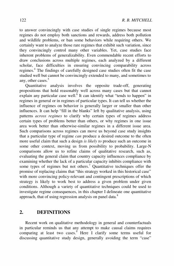
we seek to derive from the regression analysis. A regression estimates both the magnitude ( ) and likelihood (t-statistic) of regime effects as the degree of covariation between some behavioral DV and some regime-related IV. Thus, using either metric as a DV would involve regressing a qualitative assessment of regime effect on some regime characteristic to see if the regime had an effect. Although this makes little sense, other research programs have made such errors.34 Although neither set of authors has suggested using their metric to quantitatively analyze regime effectiveness, the temptation for others to do so should be avoided.

For a dependent variable to be useful in making relative judgments about disparate regimes, it must be denominated in comparable not just commonunits. Because environmental problems vary significantly in their resistance to remedy, the metric must capture both the amount of change a regime induced and how hard that amount of change was to induce.35 Consider comparing the climate change and ozone protection regimes. Assume, hypothetically, that careful analysis demonstrated that the climate regime was responsible for slowing the growth of greenhouse gas emissions by five percent whereas the ozone protection regime was responsible for actually reducing the production of ozone depleting substances (ODSs) by ninety percent, both estimated after controlling for other factors. Both regimes were “somewhat” effective, since they altered behavior. Judging which was more effective proves more challenging. On the one hand, given that the climate regime sought to stabilize greenhouse gas emissions and the ozone regime sought to eliminate ODSs, the ozone regime appears to have had a greater effect since it came closer to achieving its goal. On the other hand, changing energy consumption patterns is so much more difficult and costly than altering ODS consumption patterns that a good case can be made that even a five percent reduction would constitute a major success. Whether ultimately one would decide in favor of the climate or ozone regime, the example illustrates that we want a metric that captures both the amount of behavior change and the difficulty of inducing such change.

Assessing the relative effectiveness across regimes, as opposed to the absolute effectiveness of a regime relative to the counterfactual, requires assessing both the amount of change and the per unit effort needed to make such change. Consider these components in turn. First, we want a metric that is comparable across units of analysis. We cannot enter data on numbers of whales killed, acres of deforestation, and tons of pollutants emitted in a single regression, even though all can be expressed numerically. How should we address this problem? Regime goals differ too much to expect to create a single metric that allows convincing comparisons across all regime types. Developing a few categories of regimes based upon such criteria may allow us to make meaningful comparisons among regimes within a category. Thus,

A QUANTITATIVE APPROACH 133

we might imagine a “pollution” category for regimes addressing acid precipitation, ozone loss, climate change, and various river and ocean pollutants; a “wildlife” category for regimes addressing protection or management of endangered species, whaling, polar bears, fur seals, and various fish species; and a “habitat” category for regimes covering wetlands, world heritage sites, and desertification. One can imagine devising indicators that would allow comparison within but not across these categories: for pollutant regimes, levels of emissions; for wildlife regimes, numbers of animals killed or changes in species population; and for habitat regimes, relevant acreage.

Even when indicators can be expressed in similar units (for example, sulfur dioxide, nitrogen oxide, volatile organic compounds, ODSs, and CO2 emissions can all be expressed in tons emitted), differences in their levels make a regression using absolute levels (raw data) inappropriate. To compare across regimes, or even across countries within a regime, requires normalizing data. Often, analysts address this by using indexing (measuring relative to a given year’s level that is set as 100) or first differences (annual changes in absolute levels). To facilitate comparison across regimes, countries, and time, however, suggests normalizing absolute levels into annual percentage change scores (APCs). Like indexing, using APCs removes variance due to regime-based and country-based differences in initial levels of an activity but additionally recalibrates (and thus allows comparison across) every year. Tables 6.1 and 6.2 provide illustrative examples relevant to the first two protocols of the LRTAP regime dealing with sulfur and nitrogen oxides.

Table 6.1. Dependent variable as absolute metric.

Example: Sulfur and nitrogen oxide emissions (000s of tonnes)

Subregime Country 1988 1989 1990 1991 1992

Sulfur Belgium 354 325 372 334 318Sulfur Iceland 18 17 24 23 24Nitrogen Belgium 345 357 339 335 343Nitrogen Iceland 25 25 26 27 28

134 R. B. MITCHELL

Table 6.2. Dependent variable as annual percentage change (APC).

Example: Sulfur and Nitrogen Oxide Emissions (% change from prior year)

Subregime Country 1988 1989 1990 1991 1992

Sulfur Belgium -3.5% -8.2% 14.5% -10.2% -4.8%Sulfur Iceland 12.5% -5.6% 41.2% -4.2% 4.3%Nitrogen Belgium 2.1% 3.5% -5.0% -1.2% 2.4%Nitrogen Iceland 4.2% 0.0% 4.0% 3.8% 3.7%

The second component needed to compare regime effects in a meaningful way is per unit effort (PUE). As the ozone-climate example makes clear, simply comparing the behavioral change induced by two regimes (whether in APC or other terms) fails to account for differences in the difficulty of inducing such change.36 The challenge is to capture such differences in a way that allows comparison across regimes, countries, and time. If we accept APC as part of our DV, then it makes sense to define PUE as the difficulty of achieving a 1% change in the relevant behavior, be it emissions reduced, animals not killed, or acres protected. In pollution regimes, this corresponds to the abatement costs of a 1% emission change; in wildlife regimes, perhaps to the benefits foregone by not killing 1% of a given species or the costs of protecting an additional 1% of the population; and in habitat regimes, perhaps to the cost of protecting an additional 1% of the existing acreage. Calculating PUEs as a fixed monetary amount for a given percentage change has the virtue of avoiding the need to calculate different PUEs for different levels of the activity while still capturing the increasing marginal cost of environmental protection.37

The product of these PUE and APC constructs creates a total effort score that has several virtues as a DV for comparing regime effects. Essentially, it represents the effort made at environmental protection in “regime effort units” or REUs. Regressing REUs on a set of IVs that include at least one regime-related variable, would allow us to use the on any regime-related variable as a metric of regime effects that would, if used cautiously, be comparable across analytic units. Thus, a well-specified regression model of environmental effort (in REUs) that produced a significant t-statistic on a membership variable would allow interpretation of as the change in environmental effort induced by membership, with s being comparable across regimes. REUs also have the advantage of keeping efficiency and effects separate. Consider a regime that induced one state (with a PUE of $20 million) to spend $40 million to reduce its sulfur emissions by 2% and an equally wealthy state (but which had a PUE of $5 million) to spend $10 million to reduce its sulfur emissions by 2%. The difference in REUs ($40

A QUANTITATIVE APPROACH 135

vs. $5 million) appropriately reflects the common-sense view that the regime had more effect on the former state (it induced a more costly change in behavior) but that the latter state was more efficient in undertaking its commitments.

The argument for using REUs as DVs to allow comparison across regimes will remain largely theoretical, however, unless we can convincingly identify PUE scores for different regimes. Using REUs to compare countries within a regime requires only estimating how the costs of making a 1% change on a given environmental problem vary by country.38

Comparing the effects of different regimes or the responses of individual countries across regimes requires comparing the costs of making a 1% change on two different environmental problems. How do we assess whether the costs of inducing a 1% reduction in sulfur emissions into the atmosphere are greater or less (both on average and for specific countries) than those of inducing a 1% reduction in mercury discharges into a river? Though difficult, the problem may not be unresolvable. One approach involves limiting comparisons to regimes with relatively similar types of costs. Thus, we may feel confident comparing abatement costs for sulfur and nitrogen oxide emissions but less confident comparing them with mercury and cadmium discharges. Initial efforts may need to compare similar regimes and address more challenging comparisons after developing experience and methodologies for identifying PUE in different contexts. Despite these difficulties, when PUEs are available, REUs based on them may offer opportunities to make more meaningful cross-regime comparisons than are possible by using metrics that only capture behavioral change (e.g., APCs).

3.4 Refining the Set of Independent Variables

If we can establish a dependent variable that allows meaningful comparison across regimes (whether defined in terms of REUs, APCs, or some superior metric), analysis requires refinement of our choices of regime-related and other independent variables beyond that in the models above. On the regime-related variables side, the success of the research approach recommended here depends on scholars creating categories of regime features that simultaneously allow the testing of existing theories (e.g., realist, institutionalist, and constructivist) about how regimes influence behavior but facilitate reliable coding of real regimes into those categories. This may prove quite difficult. To take but one example, consider a project seeking to compare the effects of sanctions and rewards: how should it categorize a regime that provides financial aid but terminates that aid to countries that violate its terms? Initial research will need to start with crude

136 R. B. MITCHELL

dummy variables, refining them in the light of theoretical and empirical improvements.

Undertaking the analyses proposed here also requires careful thinking about non-regime IVs. For a model to produce interpretable explanations of changes in environmental effort, the analyst must identify a set of IVs that are sufficiently generic and generalizable that they apply to a broad range of regimes while retaining explanatory power across those regimes. Developing a good model involves the art of balancing explanatory power with generalizability, sacrificing model specificity up to a point at which doing so requires “too big” a loss in explanatory power. In part, resolving this problem requires an iterative process of selecting a set of regimes for study, attempting to apply potential IVs across those regimes, and either excluding regimes or devising a more general IV until a balance that satisfies the analyst is found.

An optimal approach to model specification may involve a generic model that includes “core” IVs that could be applied to a dataset of most regimes, a set of several intermediate models that all use these core IVs but each of which couples them with IVs that apply relatively well to their particular subset of regimes, and many regime-specific models that add additional IVs that have little applicability outside of a particular regime. The generic model could include a set of “usual suspect” IVs, such as indicators of income, economic growth, levels of economic and technological development, type of government, population, and level of environmental concern. Indeed, the environmental Kuznets curve literature provides an initial source of such variables and their indicators. Developing a list of such variables may operate best as a collective activity in which these core IVs are evaluated, critiqued, and improved as proxies that are more explanatory, more generalizable, or both are identified. Among intermediate models, one might imagine a specification for pollution treaties that added variables for development, technology, and intensity of resource use while a specification for wildlife treaties added, instead, demand for the species as exhibited by price, stock recruitment rates, and number of countries having access to the species. Further research could identify more useful distinctions, including modeling regimes that address, say, overappropriation separately from those that address underprovision problems, with indicators of administrative capacity playing a central role in the first and indicators of financial capacity playing a central role in the second.39

A QUANTITATIVE APPROACH 137

4. CONDUCTING THE EMPIRICAL ANALYSIS

Operationalizing the models suggested here engages empirical questions of sample size and the appropriate unit of analysis, the type and availability of relevant data, and the analytic techniques to be used on that data. Before proceeding, however, a few caveats deserve mention. As already noted, quantitative analysis trades off accuracy for generalizability: including more units of analysis and more observations means doing so with less knowledge and detail. We rightly place more confidence in a researcher’s assessment of the Atlantic tuna regime’s effects if she studied only that regime than if she studied it as one of ten fisheries regimes. However, we also rightly are more cautious in generalizing from an explanation of regime effects derived solely from the Atlantic tuna regime than from one derived from a larger set of regimes. If variables and models are carefully specified, quantitative methods can capture the presence or absence, strength, or quality of even quite subjective institutional and contextual variables. But, resource constraints and the need to abstract and simplify case-specific features to a sufficiently high level that they apply to a range of regimes often means that attempts to map findings to any given regime become less compelling. And, indeed, even those claims of quantitative analyses that are convincing may be too probabilistic or vague for many purposes.

4.1 Choosing Sample Size and the Unit of Analysis

Quantitative analysis of environmental regimes has been eschewed to date, at least in part, because of the assumption that there are so few environmental regimes and that they are sufficiently heterogeneous that they cannot be readily combined into a dataset susceptible to such analysis. Overcoming this apparent obstacle requires thinking carefully about the unit of analysis and sample size. Most statistical techniques require at least as many observations (remember the definitions above) as independent and control variables. Many more observations are needed to distinguish real effects from random covariation of the IV and DV, with at least 5 (and preferably 20) times as many observations as IVs usually recommended.40

Even higher ratios are recommended when the IV of interest is expected to have only a small effect on the DV or if the measurement of variables is imprecise, two problems that seem particularly likely in the study of regimes.41 If we assume that a reasonable regression model of any DV of interest requires 5 to 10 IVs, this suggests that we need data sets of at least 50 and preferably a few hundred observations.42

If we conceive of our units of analysis as involving regimes or their absence, than the heterogeneity of regimes makes it likely that we cannot

138 R. B. MITCHELL

construct a database of sufficient size and comparability to run regression analyses. Of the several hundred extant multilateral environmental treaties, most have little reliable data on any conceivable dependent variable and fewer still have comparable data for the period prior to regime formation.43

Indeed, reliable data collection often only starts upon regime formation! Quantitative analysis become possible and appropriate, however, if we consider one of three ways to increase the number of observations: examining “subregimes” rather than regimes, observing multiple years rather than one year before and one year after regime formation, and observing individual countries rather than all states as a group.

First, theoretical considerations recommend viewing regimes as composed of distinct sub-units. Evaluating the “regulatory effects of regimes” seems as valuable as evaluating “the regulatory effects of governments.” Questions like “do governments induce compliance with their regulations” or “do citizens comply with laws” entail such high levels of aggregation that they are unlikely to identify particularly compelling relationships. Assessing whether hiring more police officers “reduces traffic violations,” for example, requires either mindlessly aggregating running red lights with exceeding the speed limit or using one of these metrics in lieu of both. Yet, it is precisely the variance in speeding vs. traffic light violations that provide insight into the conditions under which people comply with traffic laws. Likewise with regimes. Most regimes involve multiple “subregimes,” i.e., analytically distinct components such as different proscriptions and prescriptions or different compliance strategies. For example, the stratospheric ozone regime can be viewed as consisting of three subregimes: one related to the ozone depleting substances (ODSs) phaseout commitments of developed states, one related to the ODS phaseout commitments of developing states, and one related to the commitments of developed states to finance the ODS phaseout of developing states. Since the effects of these subregimes are likely to vary, it makes sense to treat these as separate units of analysis so long as each has a separate indicator of its effect. Comparing the behaviors targeted by different subregimes has the additional virtue of holding many variables constant across that subset of observations derived from the same regime.

Second, because regimes do not bind equally on all states, it makes sense to use countries rather than regimes as the unit of analysis. Because some states never join certain regimes and those that do, do so at different times, we can compare the behavior of states for whom an international rule is binding to their own behavior before the rule became binding as well as to that of states who are not legally bound.

Third, whatever the dependent variable, making a convincing argument requires comparing observations of member state behavior under the regime

A QUANTITATIVE APPROACH 139

to some pre-regime period, to their behavior in similar contexts without a regime, to corresponding counterfactual thought experiments, or to the behavior of comparable nonmembers. In all of these instances, each regime-year can be considered to be a separate observation. Data on many air, land, and water pollutants as well as catch and trade statistics for various species are often available for ranges of years that span entry into force of the corresponding regimes. There is no reason to simply average data for the five years before a regime enters into force and compare it to the average for five years thereafter, when non-aggregated annual data provides greater analytic leverage.44

Taken together, these points suggest the value of defining units of analysis at the subregime-country level and recording data on all appropriate variables for all relevant years. That is, each observation would be identified in terms of subregime, country, and year.

4.2 Availability of Data

Do enough regimes with enough data exist to make quantitative analysis possible? The answer is a resounding yes, at least for some regimes. First, several data sets exist that can provide the foundation for calculating APC figures. Extensive country-year data exists on pollutants regulated under various LRTAP protocols, under the ozone regime, and under various marine and river pollution treaties. In several of these cases, data is available for ten to twenty years and for scores of countries, providing hundreds of observations for a single regime or subregime. Similarly extensive data sets exist for whaling, polar bears, various marine mammals, and many fisheries that have been regulated by international regimes. Less detailed data are available on catch, and in some instances populations (such as annual bird counts), relevant to many agreements on bird and land animal preservation. Careful coordinated research could extend this list by identifying extant datasets that contain data relevant to evaluating the effects of particular regimes or by piecing together such datasets from subsets of data developed for various scientific, rather than social scientific, purposes.

Grounds for guarded optimism also exist regarding PUE figures. Most fisheries regimes have historical catch per unit effort information.45

Researchers at IIASA have estimated abatement costs based on different scenarios for a range of countries and years that could serve as PUE estimates for European and North American acid precipitant regimes.46

Sprinz and Vaahtoranta generated country-specific abatement costs for the ozone and acid rain regimes.47 Estimates comparing the costs of environmental control across pollutants or across countries could be used to develop datasets that could serve as at least rudimentary PUE estimates for

140 R. B. MITCHELL

other regimes. The success of these analysts at estimating abatement costs using both sophisticated modeling and more crude proxy variables suggests that such efforts are likely to bear at least some fruit.

On the IV side, data on treaty entry into force and country membership are readily available for all treaties. Several analysts have already coded particular regime features for a range of environmental regimes, including data on institutional structure, monitoring, and enforcement, data that could easily be further enhanced through more systematic coding of environmental treaties.48 Country-year data are also available on a wide variety of political and economic variables that are central to any model of environmental behavior, including various permutations of GNP, population, energy use, type of government, and level of development, with most available in electronic format.

Undoubtedly, many regimes we would want to evaluate will have data for only a few years or a few countries, have data of such poor quality that it would make little sense to use it, or have no data at all. The obvious strategy in such cases is to recognize the inability to analyze such regimes in the short term and attempt to establish data collection systems that will allow such analysis in the future. An alternative possibility, however, involves a more careful and iterative search for data by identifying indicators relevant to the effectiveness of a given subregime and determining whether they are available and, reciprocally, identifying available data sets and determining to which subregimes they might be relevant. Such a process may uncover nonobvious variables that are both relevant and available to support the use of quantitative analysis to evaluate regimes. As most case study scholars know, extensive relevant data turns up for many regimes if sufficient research time is invested. A systematic attempt to work with such scholars could take advantage of their knowledge of individual data sets to create a meta-database of environmental indicators for analysis. Indeed, the belief that relevant data sets do not exist may owe more to the assumption that quantitative analysis is not possible than to the real unavailability of such data.

4.3 Using Panel Data

To take advantage of the model of regime influence, choice of units of analysis, and data resources described to this point, we must also choose appropriate analytic techniques. Defining observations in terms of subregime, country, and year allows use of panel or pooled time-series data. Although mathematically complex, the analytic techniques used to analyze panel data are conceptually easy to follow. Their major advantage lies in their ability to “take into account unobserved heterogeneity across

A QUANTITATIVE APPROACH 141

individuals and/or through time.”49 Panel data can identify the extent to which the dependent variable covaries with the regime-related independent variables after controlling both for differences across countries and for variation over time.

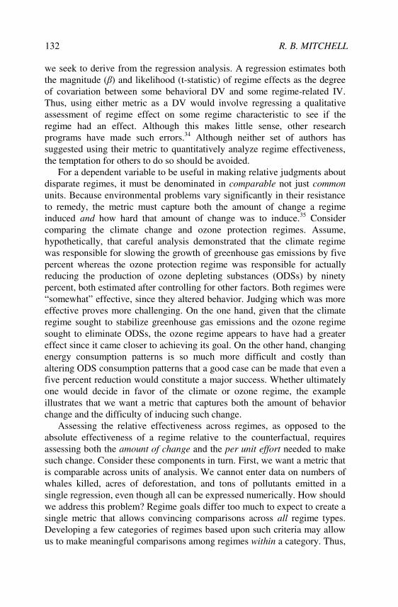
Conceptualized visually, the values of the DV fit in a matrix of rows of country-subregimes, columns of years, and cells of data, as shown in Tables 6.1 and 6.2 above. The values of IVs can be fit in corresponding matrices. If those matrices are stacked vertically, each observation would consist of drilling a single “core” through these matrices, picking up the value of the DV and the corresponding regime and other IVs for a subregime-country-year. Many IVs, for example, membership or annual percentage change in GNP, are what are called “individual time-varying variables”50 that vary by both country and year (both columns and rows differ). Other “individual time-invariant variables” vary by country but only slowly by year, such as administrative capacity or level of development, and are captured in matrices in which the value for a given country is the same for all years but those values vary across countries (rows differ but columns do not). “Period individual-invariant variables” involve time-specific differences that affect all countries equally, such as changes in regime features and changes in world oil and coal prices, and can be captured in matrices in which all countries have the same values for a given year but values vary across years (columns differ but rows do not). Tables 6.3 through 6.6 provide examples of these variables.

Table 6.3. Independent variable of interest that is individual, time-varying

Example: "Membership" based on entry into force

Subregime Country 1988 1989 1990 1991 1992

Sulfur Belgium 0 1 1 1 1Sulfur Iceland 0 0 0 0 0Nitrogen Belgium 0 0 0 1 1Nitrogen Iceland 0 0 0 0 0

Table 6.4. Control variables that are individual time-invariant

Example: Land Area (000s of sq. kilometers)

Subregime Country 1988 1989 1990 1991 1992

All Belgium 30.5 30.5 30.5 30.5 30.5All Iceland 103.0 103.0 103.0 103.0 103.0

142 R. B. MITCHELL

Table 6.5. Control variables that are period, individual-invariant

Example: World Oil Price Index ($/bbl)

Subregime Country 1988 1989 1990 1991 1992

All Belgium 81.2 107.7 123.5 120.7 131.3All Iceland 81.2 107.7 123.5 120.7 131.3

Table 6.6. Control variables that are individual, time-varying

Example: GNP per capita (000s of constant 1995$)

Subregime Country 1988 1989 1990 1991 1992

All Belgium 24.3 25.1 25.7 26.1 26.4All Iceland 25.5 25.5 25.6 25.7 24.7

What advantages does analysis of such panel data have for evaluating the effects of regimes? Consider efforts to estimate how membership influences state behavior. Any analysis of the influence of regimes on state behavior must address an inherent problem of endogeneity: agreements are signed only when states, and by those states that, are ready to limit environmental harm. Therefore, by definition but for reasons unrelated to IEAs, the activities of member states will differ both from their prior behavior and from that of nonmember states. Cases where different treaty provisions correlate with behaviors or environmental quality may be mere reflections of underlying differences in the problem being addressed or other factors. Addressing these obstacles that require careful theorizing and the use of analytic techniques that are available but are only beginning to be applied to the task.

Cross-section data (looking at a range of countries in a given year) would estimate the effect of membership by comparing member behavior to nonmember behavior, failing to address the likelihood that member countries differ in systematic ways from nonmembers. Such data makes it difficult to decipher whether “better” behavior by members reflects the influence of membership or the fact that those most willing and able to alter their behavior become members. Even with proxies for such willingness or ability included in the model, the possibility remains that member and nonmembers differ in some systematic but unobserved way. In contrast, time-series data estimates the membership effect by comparing the behavior of states as members to their behavior as nonmembers, controlling for other factors. This approach ignores the possibility that other influences that occur contemporaneously with becoming a member (for example, the end of the

A QUANTITATIVE APPROACH 143

Cold War in the LRTAP sulfur case) explain the change in behavior. Regression using time-series data cannot distinguish whether membership or other coincidental factors are responsible for behavioral differences.

Panel data begins to address the endogeneity problem by taking advantage of both types of variation simultaneously. Panel data uses changes in nonmember behavior over time to estimate how time-varying factors would have effected member behavior, thereby avoiding erroneously attributing those effects to membership. Panel data controls for country-specific factors by using changes in behavior during the period in which a country was not a regime member to estimate how its behavior would have been driven by non-regime factors when it was a member, thereby avoiding erroneously attributing those effects to membership. Thus, panel data improves our estimate of regime effects by more effectively separating regime effects from those due to time or country variables.51 Panel data analysis also has advantages in deriving causal inferences, assessing measurement errors in variables, correcting for autocorrelation, evaluating the model specification, and addressing data heteroskedasticity.52 Even more progress can be made in this regard by employing statistical methods explicitly designed to address endogeneity problems, e.g., two-stage least squares models.53

5. CONCLUSION

Quantitative analysis offers opportunities to investigate certain aspects of regime effects for which qualitative techniques are less well-suited. Although factor analysis, contingency tables, and other techniques are certainly possible and should be explored, the present chapter has investigated the contribution that regression analysis using panel data could make to determining whether, which type of, and under what conditions, regimes wield influence. Studies that collect data on a range of regimes provide valuable means for identifying general trends across regimes, evaluating whether some regimes are more effective than others, and determining how non-regime factors condition the effects of a particular type of regime.

Stating that quantitative techniques can complement qualitative analyses and contribute to the regime consequences research project does not mean, however, that undertaking such analyses will be easy. Indeed, the foregoing argument has sought to identify and clarify the numerous theoretical and empirical obstacles to using quantitative analysis to answer questions central to research on regime effects. Devising a dependent variable that would allow meaningful comparison across regimes requires careful attention to

144 R. B. MITCHELL

creating a comparable metric of behavioral change and a comparable metric of the difficulty of inducing behavioral change. Likewise, representing regime influence in the model requires careful specification if we are to determine how regimes influence members, how they influence nonmembers, and how their influences differ across the two. Comparing across regimes also requires careful attention to specification of non-regime control variables. A model designed to apply to all regimes is likely to produce weak and perhaps uninterpretable estimates of regime effects; one designed to apply well to a single regime precludes comparison across regimes. Intermediate models specified to explain the variation in the dependent variable across a set of regimes that are selected for similarity in their predicted impacts may reach the right balance between these too-generic and too-specific extremes. Applying such a model to panel data using subregime-country-years as our observations allows us to control for variables in ways that more aggregated analyses cannot. Such data appears to be available, at least for enough regimes to make the enterprise worth pursuing. A well-specified model and corresponding data would allow us to evaluate whether regimes influence states, whether they do so in ways that would be unlikely to have occurred by chance, which ones do so better than others, and a variety of other as yet unidentified but important questions.

ACKNOWLEDGEMENTS

An earlier version of this chapter appeared as Ronald B. Mitchell, ‘A Quantitative Approach to Evaluating International Environmental Regime’, Global Environmental Politics, 2:4 (November 2002), pp. 58-83. © by the Massachusetts Institute of Technology. The chapter has benefited greatly from comments from Arild Underdal, Oran Young, Detlef Sprinz, and participants in a conference on “Regime Consequences: Methodological Challenges and Research Strategies” hosted by the Centre for Advanced Study of the Norwegian Academy of Science and Letters in June 2000. This chapter was completed with the generous support of a Sabbatical Fellowship in the Humanities and Social Sciences from the American Philosophical Society and a 2002 Summer Research Award from the University of Oregon.

A QUANTITATIVE APPROACH 145

NOTES

1 For some exceptions, see Meyer et al. 1997; Downs et al. 1998; and Miles et al. 2001. Several scholars have put together data sets that code a variety of parameters for a range of environmental treaty regimes. The International Regimes Database (IRD) has begun pulling together an extensive set of data on thirty different treaties which, once completed, will constitute a significant advance in the data that will be available to the policy and scholarly community. Haas and Sundgren examined trends in environmental treaty making (Haas and Sundgren 1993). Dmitris Stevis has collected data on membership and characteristics of international environmental institutions (Stevis 1999).

2 Downs et al. 1996. 3 Princen 1996. 4 Brown Weiss and Jacobson collected extensive information on compliance and its

determinants for ten countries and five different treaties (Brown Weiss and Jacobson 1998). Miles et al. have developed a database of 44 cases involving regime phases or components (Miles et al. 2001).

5 Mitchell and Bernauer 1998. 6 Thus, the convincing, if contested, quantitative finding that democratic states rarely go to

war against each other proves unsatisfactory in explaining why any particular war occurs. 7 Haas et al. 1993; Brown Weiss and Jacobson 1998; and Victor et al. 1998. 8 For an initial application of this approach, see Mitchell 2003a. 9 King et al. 1994; Fearon 1991; and Biersteker 1993. 10 See Ragin and Becker 1992; Galtung 1967; King et al. 1994; Yin 1994. 11 King et al. 1994, 52. 12 Krasner 1983. 13 Haas et al. 1993; Mitchell, 1994; Brown Weiss and Jacobson 1998; Victor et al. 1998,

Young 1997; Young 1999a; Miles et al. 2001. 14 See Young 1999a; Helm and Sprinz 2000; Miles et al. 2001. 15 Underdal and Young this volume; see also Young 2002. 16 Thus, as a hypothetical example, a study that used the end of the Cold War as a control for

the contextual variable “polarity” might identify that the regimes in the study sample had only a “small” average effect when polarity was controlled for. Including a polarity-regime interaction term, however, might demonstrate that this “small” effect was the average of a quite large effect of regimes in the post-Cold War uni-polar world and no effect in the Cold War bi-polar world.

17 Mitchell 1994; Mitchell 1996; Chayes and Chayes 1993; Brown Weiss and Jacobson 1998. 18 Young 1999a; Young 1999b; Victor et al. 1998; Miles et al. 2001; Stokke 1997; Wettestad

1999. 19 Levy 1993; Levy 1995; Sprinz 1998. 20 For a review of this literature, see Harbaugh et al. 2001. 21 A more refined counterfactual might subtract 1 from emissions forecast by the model

using each states' actual values for all the IVs. The impact of regime membership for that state would then consist of the difference between its actual emissions and the emissions forecast by this method.

22 Helm and Sprinz 2000; Sprinz and Helm 1999. 23 The criteria usually viewed as necessary to infer a causal relationship between A and B are

demonstrating “relationship” (co-variation of the values of A with the values of B), “time precedence” (changes in A precede changes in B), and “nonspuriousness” (the ability to rule out other possible causal variables) (Asher 1976, 11; Kenny 1979, 3-5).

146 R. B. MITCHELL

24 Of course, a fully accurate interpretation of the in this way requires that the analyst have paid careful attention to multi-collinearity, heteroskedasticity, omitted variable bias, and a variety of additional statistical concerns.

25 Meaningful comparison of the magnitude of coefficients requires, inter alia, careful attention to the order in which variables enter the regression equation, as noted in any standard statistics textbook.

26 The adjusted R2 is conceptually identical but corrects this estimate to reflect the fact that adding more IVs to a regression equation can increase the R2 even if the additional IVs do not have any significant correlation with the DV.

27 Chayes and Chayes 1995; Downs et al. 1996. A more accurate depiction of the theoretical claims made by Downs et al. would need, at a minimum, to reflect their view that the importance of sanctions depends on the ambitiousness of the regime goals which they refer to as “depth of cooperation.”

28 1 represents the change in behavior induced in members of a regime, controlling for type of regime (i.e., comparing members of sanction-based regimes to nonmembers of those regimes, and members of non-sanction-based regimes to nonmembers of those regimes).

29 2 represents the change in behavior that correlates with variation in whether a regime has sanctions or not, controlling for membership (i.e., comparing members of sanction-based regimes to members of other regimes, and nonmembers of sanction-based regimes to nonmembers of other regimes).

30 Brown Weiss and Jacobson 1998, 528-530. 31 Sprinz and Helm 1999; Helm and Sprinz 2000. 32 Sprinz and Helm 1999, 365. 33 Underdal 2001, 4. 34 Indeed, the seminal quantitative work on economic sanctions made precisely this mistake,

regressing a DV that included “the contribution made by sanctions to a positive outcome” on whether sanctions were imposed or not to determine whether sanctions influence state behavior (Hufbauer et al. 1990).

35 Miles et al. 2001; Young 1999b; Wettestad 1999. 36 The notion of differences in the difficulty of inducing behavioral change has many

similarities to Miles et al. (2001) notion of problem “malignity.” 37 A pollution PUE of $500 implies that inducing a country to reduce its pollution from

10,000 units to 9,900 units (100 units or 1%) will cost a regime $500 but inducing a country to reduce its pollution from 1,000 units to 900 units (100 units but 10%) will cost the regime $5,000 ($500 * 10%).

38 Indeed, the assumption that abatement costs, and by implication PUE scores, vary by country underlies the flexibility mechanisms designed into the Climate Change Convention.

39 Ostrom 1990; Mitchell 1999. 40 Tabachnick and Fidell 1989, 129. 41 Tabachnick and Fidell 1989, 129. 42 Statistical power analysis confirms these general rules of thumb, suggesting that a

regression model using 8 independent variables, a statistical significance test (i.e., ) of .05, and a power criterion of .80 would need a sample of 107 to detect a “medium” effect size and a sample of over 700 to detect a “small” effect size (Cohen 1992, 155-159). 43 Mitchell 2003b.

44 Murdoch et al. 1997. 45 Peterson 1993. 46 Alcamo et al. 1990.

A QUANTITATIVE APPROACH 147

47 Sprinz and Vaahtoranta 1994. 48 For example, databases created by Peter Haas, Dimitris Stevis, Edith Brown Weiss and

Harold Jacobson, and the International Regimes Database all have systematic codings of several variables for various environmental treaties. See Haas and Sundgren 1993, 401-429; Brown Weiss and Jacobson 1998; Victor et al. 1998; and Stevis 1999.

49 Hamerle and Ronning 1995. 50 Hamerle and Ronning 1995; Finkel 1995. 51 Finkel 1995. 52 Finkel 1995. 53 Mitchell 2003a.

REFERENCES

Alcamo, J., Shaw, R. and Hordijk, L. (eds.) (1990) The RAINS Model of Acidification: Science and Strategies in Europe, Kluwer Academic Publishers, Dordrecht.

Asher, H. B. (1976) Causal Modeling. Sage Publications, CA. Biersteker, T. (1993) Constructing Historical Counterfactuals to Assess the Consequences of

International Regimes: The Global Debt Regime and the Course of the Debt Crisis of the 1980s, in Regime Theory and International Relations, edited by V. Rittberger, Oxford University Press, New York, 315–338.

Brown Weiss, E. and Jacobson, H. K. (eds.) (1998) Engaging Countries: Strengthening Compliance with International Environmental Accords, MIT Press, Cambridge, MA.

Chayes, A. and Chayes, A. H. (1993) On Compliance, International Organization47: 175–205. Chayes, A. and Chayes, A. H. (1995) The New Sovereignty: Compliance with International

Regulatory Agreements, Harvard University Press, Cambridge, MA. Cohen J. (1992) A Power Primer, Psychological Bulletin 112: 155–9. Downs, G. W., Rocke, D. M. and Barsoom, P. N. (1996) Is the Good News about Compliance

Good News about Cooperation? International Organization 50: 379–406. Downs, G. W., Rocke, D. M. and Barsoom, P. N. (1998) Managing the Evolution of

Cooperation, International Organization 52: 397–419. Eckstein, H. (1975) Case Study and Theory in Political Science, in F. Greenstein and N. Polsby (eds.) Handbook of Political Science, Vol. 7, Strategies of Inquiry, Addison-Wesley

Press, Reading, MA, 79–137. Fearon, J. D. (1991) Counterfactuals and Hypothesis Testing in Political Science, World Politics 43: 169–195. Finkel, S. E. (1995) Causal Analysis with Panel Data, Sage Publications, CA. Galtung, J. (1967) Theory and Methods of Social Research, Columbia University Press, New York. Haas, P. M., and Sundgren, J. (1993) Evolving International Environmental Law: Changing

Practices of National Sovereignty, in N. Choucri (ed.) Global Accord: Environmental Challenges and International Responses, MIT Press, Cambridge, MA, 401–429.

Haas, P. M., Keohane, R. O. and Levy, M. A. (eds.) (1993) Institutions for The Earth: Sources of Effective International Environmental Protection, MIT Press, Cambridge, MA.

Hamerle, A., and Ronning, G. (1995) Panel Analysis for Qualitative Variables, in G. Arminger, C. C. Clogg, M. E. Sobel, (eds.) Handbook of Statistical Modeling for the

Social and Behavioral Sciences, Plenum Press, New York, 401–451.

148 R. B. MITCHELL

Harbaugh, W., Levinson, A. and Wilson, D. (2000) Re-examining the Empirical Evidence for an Environmental Kuznets Curve, National Bureau of Economic Research, Cambridge, MA.

Helm, C. and Sprinz, D. (2000) Measuring the Effectiveness of International Environmental Regimes, Journal of Conflict Resolution 44: 630–652.

Hufbauer, G. C., Schott, J. J. and Elliott, K. A. (1990) Economic Sanctions Reconsidered: History and Current Policy, Institute for International Economics, Washington, DC.

Kenny, D. A. (1979) Correlation and Causality, John Wiley and Sons, New York. King, G., Keohane, R. O. and Verba., S. (1994) Designing Social Inquiry: Scientific Inference

in Qualitative Research, Princeton University Press. Krasner, S. (1983) International Regimes, Cornell University Press, Ithaca, New York. Levy, M. A. (1995) International Cooperation to Combat Acid Rain, in H. O. Bergesen and G. Parmann (eds.) Green Globe Yearbook: An Independent Publication on Environment and

Development, Oxford University Press, NC, 59–68. Levy, M. A. (1993) European Acid Rain: The Power of Tote-Board Diplomacy, in P. Haas, R. O. Keohane, and M. Levy (eds.) Institutions for the Earth: Sources of Effective

International Environmental Protection, MIT Press, Cambridge, MA, 75–132. Meyer, J. W., Frank, D. J., A. Hironaka, A. , Schofer, E. and Tuma, N. B. (1997) The Structuring of a World Environmental Regime, 1870 – 1990, International Organization

51: 623–629. Miles, E. L., Underdal, A., Andresen, S., Wettestad, J., Skjaerseth, J. B. and Carlin, E. M.

(eds.) 2001, Environmental Regime Effectiveness: Confronting Theory with Evidence,MIT Press, Cambridge, MA. Mitchell, R. B. and Bernauer, and T. (1998) Empirical Research on International

Environmental Policy: Designing Qualitative Case Studies, Journal of Environment and Development 7: 4–31.

Mitchell, R. B. (1996) Compliance Theory: An Overview, in J. Cameron, J. Werksman and P. Roderick (eds.) Improving Compliance with International Environmental Law, Earthscan,

London, 3–28. Mitchell, R. B. (1994) Intentional Oil Pollution at Sea: Environmental Policy and Treaty

Compliance, MIT Press, Cambridge, MA. Mitchell, R. B. (1999) International Environmental Common Pool Resources: More Common

than Domestic but More Difficult to Manage, in J. S. Barkin and G. Shambaugh (eds.)Anarchy and the Environment: The International Relations of Common Pool Resources,SUNY Press, Albany, NY.

Mitchell, R. B. (2003a) The Relative Effects of Environmental Regimes: A Quantitative Comparison of Four Acid Rain Protocols, paper presented at the International Studies Association Conference, Portland, OR.

Mitchell, R. B. (2003b) International Environmental Agreements: A Survey of Their Features, Formation, and Effects, Annual Review of Environment and Resources 28.

Murdoch, J. C., Sandler, T. and Sargent, K. (1997) A Tale of Two Collectives: Sulphur Versus Nitrogen Oxides Emission Reduction in Europe, Economica 64: 281–301.

Ostrom, E. (1990) Governing the Commons: The Evolution of Institutions for Collective Action, Cambridge University Press.

Peterson, M. J. (1993) International Fisheries Management, in P. Haas, R. O. Keohane and M. Levy, Institutions For The Earth: Sources of Effective International Environmental

Protection, MIT Press, Cambridge, MA, 249–308. Princen, T. (1996) The Zero Option and Ecological Rationality in International

Environmental Politics, International Environmental Affairs 8: 147–176.

A QUANTITATIVE APPROACH 149

Ragin, C. C. and Becker, H. S. (1992) What is a Case? Exploring the Foundations of Social Inquiry, Cambridge University Press.

Sprinz, D. and Helm, C. (1999) The Effect of Global Environmental Regimes: A Measurement Concept, International Political Science Review 20: 359–369. Sprinz, D. and Vaahtoranta, T. (1994) The Interest-Based Explanation of International

Environmental Policy, International Organization 48: 77–105. Sprinz, D. (1998) Domestic Politics and European Acid Rain Regulation, in A. Underdal (ed.)

The Politics of International Environmental Management, Kluwer Academic Publishers, Dordrecht, 41–66.

Stevis, D. (1999) Email communication. Stokke, O. S. (1997) Regimes as Governance Systems, in O. R. Young (ed) Global

Governance: Drawing Insights from the Environmental Experience, MIT Press, Cambridge, MA, 27–63.

Tabachnick, B. G. and Fidell, L. S. (1989) Using Multivariate Statistics, HarperCollins, New York. Underdal, A. (2001) Conclusions: Patterns of Regime Effectiveness, in E. L. Miles et al (eds.)

Environmental Regime Effectiveness: Confronting Theory with Evidence, MIT Press, Cambridge, MA.

Underdal, A. and Young, O. R. (eds.) (forthcoming) Regime Consequences: Methodological Challenges and Research Strategies, Kluwer Academic Publishers, Dordrecht.

Victor, D. G., Raustiala, K. and Skolnikoff, E. B. (eds.) (1998) The Implementation and Effectiveness of International Environmental Commitments, MIT Press, Cambridge, MA.

Wettestad, J. (1999) Designing Effective Environmental Regimes: The Key Conditions,Edward Elgar, Cheltenham, UK.

Yin, R. (1994) Case Study Research: Design and Methods, 2nd ed., Sage Publications, CA. Young, O. R. (ed.) (1997) Global Governance: Drawing Insights from the Environmental

Experience, MIT Press, Cambridge, MA. Young, O. R., (ed.) (1999a) Effectiveness of International Environmental Regimes: Causal

Connections and Behavioral Mechanisms, MIT Press, Cambridge, MA. Young, O. R., (1999b) Governance in World Affairs, Cornell University Press, Ithaca, New

York. Young, O. R. (2002) The Institutional Dimensions of Environmental Change: Fit, Interplay,

and Scale, MIT Press, Cambridge, MA.