CHAPTER 51 TESTING - cise.ufl.edu

Data Structures, Algorithms, & Applications in JavaCopyright 1999 Sartaj Sahni

CHAPTER 51_________

TESTING

This material is essentially Chapter 9 of the book Software Development in Pascal bySartaj Sahni, NSPAN Printing and Publishing, 1993. It is reproduced here with permis-sion of the publisher.

51.1 INTRODUCTION

Test data is a set of inputs that may be provided to a program to check itsbehavior. For example, each run of the quadratic roots program, Program 1.30 ofthe text, requires values for the three variables: a, b, and c. A possible set ofinputs that can be used to test this program is (2, 3, 4) (i.e., a = 2, b = 3, and c =4). So, (2, 3, 4) may be used as test data for this program. A test data set (oftenabbreviated test set) is a collection of test data. For the quadratic roots program,{(2, 3, 4), (1, 5, −2), (3.2, 4.5, 8.2), (−2.6, −9.1, 8.4)} is a possible test set. If thistest set is used, the program will be executed four times; once with each of thefour sets of inputs in the test set.

Testing is the process of executing the program code in the target environ-ment using test data. The behavior of the program on this test data is comparedwith that predicted by the program specifications. Hence, for a set of inputs to be

1

-- --

2 Chapter 51 Testing

used as test data, it is essential that the behavior of a correct program run withthat set of inputs be known. Thus, to use the above test set for Program 5.3, wemust know the roots of each of the four quadratic equations defined by the foursets of input data.

The number of different inputs that can be provided to a program is gen-erally so large that no practical amount of testing can establish the correctness ofthe program. For the quadratic roots problem, the number of different quadraticequations that can be input is infinite in theory. In practice, this number is finitethough very large. If 16 bits are used to represent each of the inputs a, b, c(including sign, magnitude, and exponent), then only 216 different values are pos-sible for each. Hence, the number of different sets of inputs is only 248 . If ourtarget computer can run Program 1.30 220 = 1, 048, 576 times a second, it willtake 228 seconds ≈ 8.5 years to try out all 248 sets of inputs. It is impractical totest Program 1.30 on all possible inputs that may be provided to it. Hence, test-ing must often be limited to a (very small) subset of all possible inputs. Testingwith this subset cannot conclusively establish the correctness of the program. Asa result, the objective of testing is not to establish correctness but to expose thepresence of errors. The test set must be chosen in such a way as to expose anyerrors that may be present in the program.

To test a program, we need the following:

1. Access to the target environment. This environment consists of both thehardware and software environment under which the program is to work.

a. The hardware environment is clearly important. A program that runscorrectly on a PC may malfunction on a workstation (or the reverse).A program may function correctly on a PC that has 32MB of memorybut fail on one that has only 16MB of memory. The screen utilitiesmay work correctly on a PC with a medium resolution monitor butincorrectly on the same computer with a high resolution monitor.

b. The software environment includes the operating system under whichthe program is to run. It is quite possible for a program to functioncorrectly under one operating system on a particular computer andfail to run under a different operating system on the same computer.For example, a program that runs correctly under Windows 95 mayfail to run correctly when the operating system is changed to Win-dows NT. This may occur even though no change is made to thehardware environment. In fact, it is quite possible for a program torun correctly under one version of an operating system and to pro-duce errors on another version of the same operating system. A C++program may compile correctly using one compiler but may generatecompiler errors when another compiler is used.

For the above reasons, it is essential to test the program in the environmentin which it is to be eventually used.

-- --

Section 51.1 Introduction 3

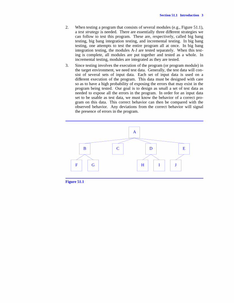
2. When testing a program that consists of several modules (e.g., Figure 51.1),a test strategy is needed. There are essentially three different strategies wecan follow to test this program. These are, respectively, called big bangtesting, big bang integration testing, and incremental testing. In big bangtesting, one attempts to test the entire program all at once. In big bangintegration testing, the modules A-J are tested separately. When this test-ing is complete, all modules are put together and tested as a whole. Inincremental testing, modules are integrated as they are tested.

3. Since testing involves the execution of the program (or program module) inthe target environment, we need test data. Generally, the test data will con-sist of several sets of input data. Each set of input data is used on adifferent execution of the program. This data must be designed with careso as to have a high probability of exposing the errors that may exist in theprogram being tested. Our goal is to design as small a set of test data asneeded to expose all the errors in the program. In order for an input dataset to be usable as test data, we must know the behavior of a correct pro-gram on this data. This correct behavior can then be compared with theobserved behavior. Any deviations from the correct behavior will signalthe presence of errors in the program.

F G H I J

B C D E

A

Figure 51.1

-- --


51.2 MODULE TESTING STRATEGIES

51.2.1 Big Bang Testing

In big bang testing, all testing is performed on the program as a whole. Whenthis approach is used on the program of Figure 51.1, the entire program is com-piled and executed with test data. If the behavior of the program disagrees withthe expected behavior on any one of the test data, then the cause of thisdiscrepancy may be in any of the modules A-J. To detect this cause, one has tocheck the logic and interface of each of the modules in some systematic order.Once the cause of the error has been identified and removed, the program isrecompiled and run on the test data.

Some of the disadvantages of big bang testing are:

1. One has to handle module interfacing problems as well as logic errorswithin a module at the same time. Module interfacing problems includesuch things as a discrepancy between the number and/or type of formal andactual parameters, discrepancy in the form in which a module expects data(say sorted) and the form in which it is actually provided (say unordered)by the invoking module, formal parameters that need to pass computedvalues back to the invoking module may not have been identified as beingof type var in the module declaration, etc.

2. When the behavior of the program on a test run differs from the expectedbehavior, the cause of the error could be in any of the modules. Findingthis cause requires the tester to trace through the entire program. Hence,debugging is expensive.

3. Big bang testing is expensive in terms of the computer time and memoryrequired. Each time a bug is found and ‘‘fixed’’, the entire program getsrecompiled (unless an incremental compiler is in use). For large programs,this recompilation is very expensive. When an incremental compiler is inuse, only the module (or part of the module) that has been changed needs tobe recompiled. Still, to test the corrected program, the entire program isloaded into memory and run. The result may be the detection of anotherbug in the same module as earlier. It would be cheaper to get as many bugsas possible out of each of the modules by testing them separately and thentesting the program as a whole.

51.2.2 Big Bang Integration Testing

In big bang integration, one tests each of the modules independently. Each ofthe 10 modules A-J of Figure 51.1 are tested independent of the others. Whenthis testing has been completed, the modules are put together and the entire pro-gram tested. Since the individual modules have been tested before being

-- --

Section 51.2 Module Testing Strategies 5

integrated together, one expects that all logic errors within the modules havebeen detected and corrected before the testing of the integrated program com-mences. Consequently, when the integrated program is tested, one only expectsto discover problems related to the interfaces. In practice, because testing is lim-ited to a subset of all possible inputs, logic errors within a module may bedetected even when the integrated program is being tested.

The big bang integration testing strategy clearly overcomes some of thedifficulties associated with big bang testing. We make the following observa-tions with regard to this test strategy:

1. Ideally, all logic errors in a module will be detected when the module isbeing tested independent of the others. Debugging is easier as it is local-ized to the module under test.

2. Module interface problems have to be dealt with only after individualmodules have been tested. In the ideal case, all bugs found when theintegrated program is being tested will be related to module interface prob-lems alone.

3. The testing of large programs using this approach is expected to requireless computer time. The full memory requirements of the program areneeded only when the integrated program is being tested.

4. There is significant potential for parallel testing. To test one module, weneed not wait for the testing of another to complete. Given enough person-nel, all modules can be tested in parallel. So, this phase of the testing canbe completed quickly.

Big bang integration testing, however, has problems of its own. One ofthese is a left over from big bang testing. All problems associated with integrat-ing the modules are tackled simultaneously. Thus, while resolving the interfaceproblems between modules B and F, the entire program is being repeatedly com-piled and executed. It is cheaper to resolve these problems independent of theproblems between the remaining interfaces.

A more subtle difficulty with this approach is one that doesn’t exist whenthe big bang approach is used. This has to do with actually testing one moduleindependent of the others. For example, to test the module B of Figure 51.1, weneed to write three modules. First, we need to write a module that invokes B.This module is called a driver. In some cases, it is sufficient for the drivermodule to simply contain a statement to invoke B. In other cases, the driverneeds to first set up the environment that B is to work with and then when B hascompleted, it is necessary for the driver to output the results (if any) for com-parison with the expected results.

In addition to the driver for B, we need modules that simulate the modulesF and G. These modules are called stubs. The stub modules need to provide theresults that would otherwise have been provided by modules F and G.

-- --


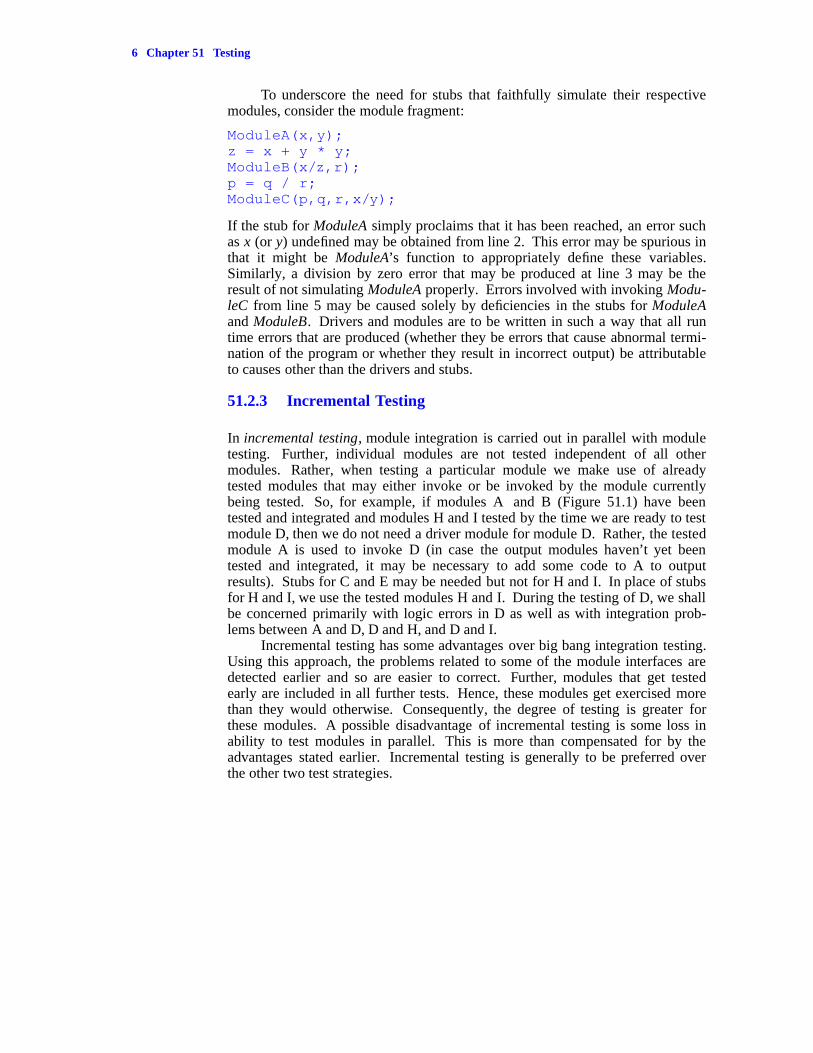
To underscore the need for stubs that faithfully simulate their respectivemodules, consider the module fragment:

ModuleA(x,y);z = x + y * y;ModuleB(x/z,r);p = q / r;ModuleC(p,q,r,x/y);

If the stub for ModuleA simply proclaims that it has been reached, an error suchas x (or y) undefined may be obtained from line 2. This error may be spurious inthat it might be ModuleA’s function to appropriately define these variables.Similarly, a division by zero error that may be produced at line 3 may be theresult of not simulating ModuleA properly. Errors involved with invoking Modu-leC from line 5 may be caused solely by deficiencies in the stubs for ModuleAand ModuleB. Drivers and modules are to be written in such a way that all runtime errors that are produced (whether they be errors that cause abnormal termi-nation of the program or whether they result in incorrect output) be attributableto causes other than the drivers and stubs.

51.2.3 Incremental Testing

In incremental testing, module integration is carried out in parallel with moduletesting. Further, individual modules are not tested independent of all othermodules. Rather, when testing a particular module we make use of alreadytested modules that may either invoke or be invoked by the module currentlybeing tested. So, for example, if modules A and B (Figure 51.1) have beentested and integrated and modules H and I tested by the time we are ready to testmodule D, then we do not need a driver module for module D. Rather, the testedmodule A is used to invoke D (in case the output modules haven’t yet beentested and integrated, it may be necessary to add some code to A to outputresults). Stubs for C and E may be needed but not for H and I. In place of stubsfor H and I, we use the tested modules H and I. During the testing of D, we shallbe concerned primarily with logic errors in D as well as with integration prob-lems between A and D, D and H, and D and I.

Incremental testing has some advantages over big bang integration testing.Using this approach, the problems related to some of the module interfaces aredetected earlier and so are easier to correct. Further, modules that get testedearly are included in all further tests. Hence, these modules get exercised morethan they would otherwise. Consequently, the degree of testing is greater forthese modules. A possible disadvantage of incremental testing is some loss inability to test modules in parallel. This is more than compensated for by theadvantages stated earlier. Incremental testing is generally to be preferred overthe other two test strategies.

-- --


When carrying out an incremental test of a program, one has to determinethe order in which the modules are to be tested and integrated. Two popular stra-tegies for this are: top down and bottom up. These are discussed below:

Top Down Incremental Testing

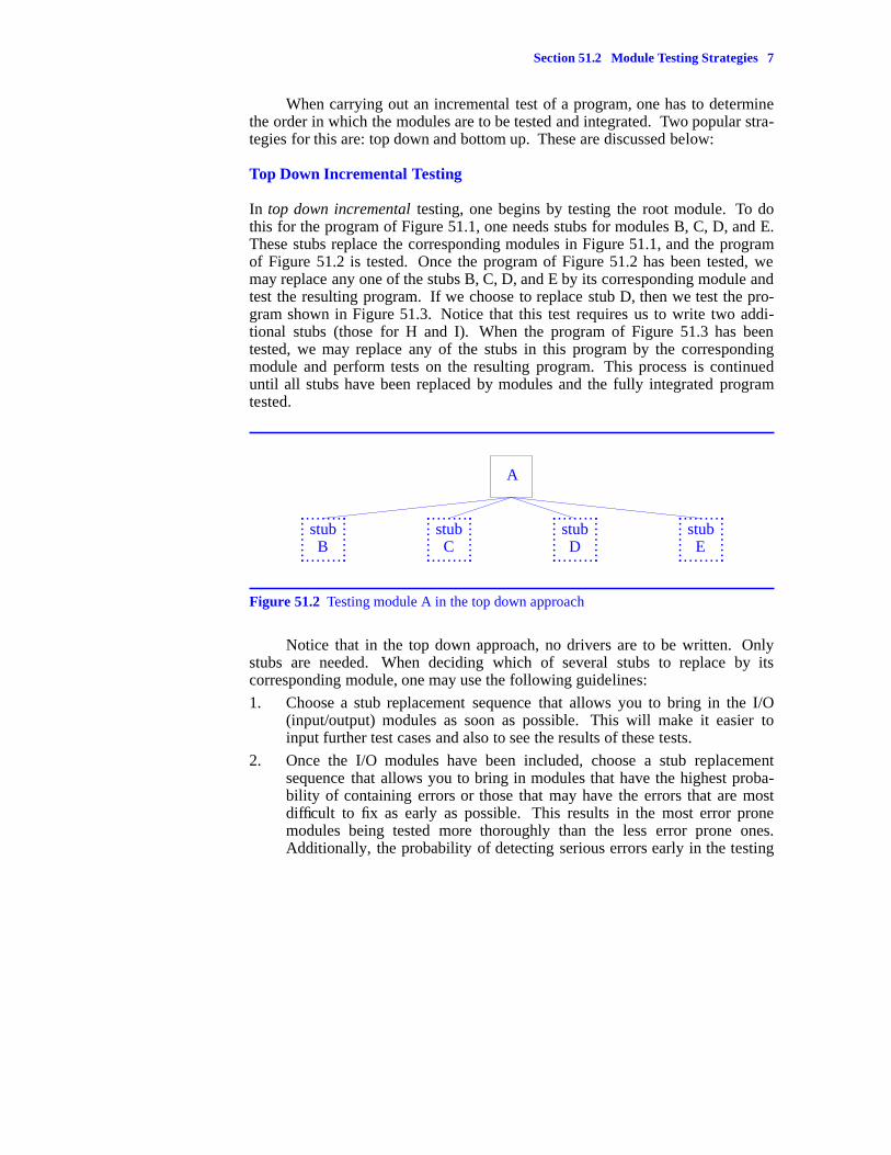
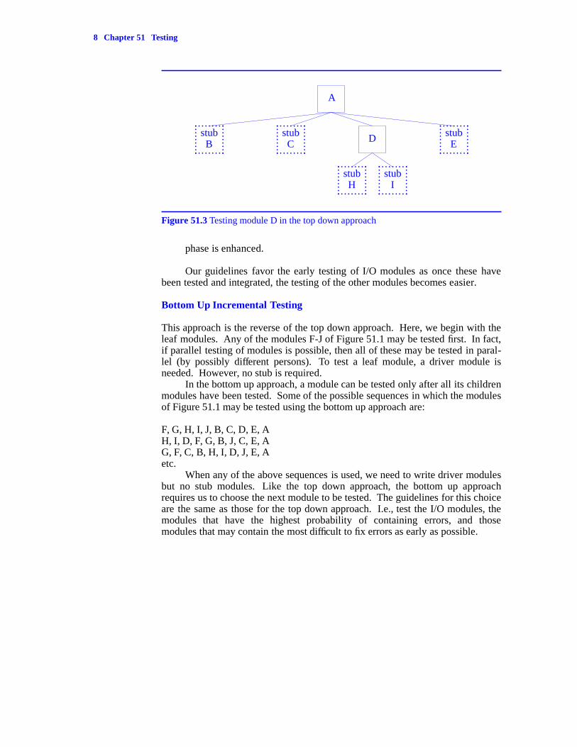
In top down incremental testing, one begins by testing the root module. To dothis for the program of Figure 51.1, one needs stubs for modules B, C, D, and E.These stubs replace the corresponding modules in Figure 51.1, and the programof Figure 51.2 is tested. Once the program of Figure 51.2 has been tested, wemay replace any one of the stubs B, C, D, and E by its corresponding module andtest the resulting program. If we choose to replace stub D, then we test the pro-gram shown in Figure 51.3. Notice that this test requires us to write two addi-tional stubs (those for H and I). When the program of Figure 51.3 has beentested, we may replace any of the stubs in this program by the correspondingmodule and perform tests on the resulting program. This process is continueduntil all stubs have been replaced by modules and the fully integrated programtested.

stubB

..... . . . ............................

stubC

..... . . . ............................

stubD

..... . . . ............................

stubE

..... . . . ............................

A

Figure 51.2 Testing module A in the top down approach

Notice that in the top down approach, no drivers are to be written. Onlystubs are needed. When deciding which of several stubs to replace by itscorresponding module, one may use the following guidelines:

1. Choose a stub replacement sequence that allows you to bring in the I/O(input/output) modules as soon as possible. This will make it easier toinput further test cases and also to see the results of these tests.

2. Once the I/O modules have been included, choose a stub replacementsequence that allows you to bring in modules that have the highest proba-bility of containing errors or those that may have the errors that are mostdifficult to fix as early as possible. This results in the most error pronemodules being tested more thoroughly than the less error prone ones.Additionally, the probability of detecting serious errors early in the testing

-- --


stubH

..... . . . ............................

stubI

.... . . . . ............................

stubB

..... . . . ............................

stubC

..... . . . ............................

D stubE

..... . . . ............................

A

Figure 51.3 Testing module D in the top down approach

phase is enhanced.

Our guidelines favor the early testing of I/O modules as once these havebeen tested and integrated, the testing of the other modules becomes easier.

Bottom Up Incremental Testing

This approach is the reverse of the top down approach. Here, we begin with theleaf modules. Any of the modules F-J of Figure 51.1 may be tested first. In fact,if parallel testing of modules is possible, then all of these may be tested in paral-lel (by possibly different persons). To test a leaf module, a driver module isneeded. However, no stub is required.

In the bottom up approach, a module can be tested only after all its childrenmodules have been tested. Some of the possible sequences in which the modulesof Figure 51.1 may be tested using the bottom up approach are:

F, G, H, I, J, B, C, D, E, AH, I, D, F, G, B, J, C, E, AG, F, C, B, H, I, D, J, E, Aetc.

When any of the above sequences is used, we need to write driver modulesbut no stub modules. Like the top down approach, the bottom up approachrequires us to choose the next module to be tested. The guidelines for this choiceare the same as those for the top down approach. I.e., test the I/O modules, themodules that have the highest probability of containing errors, and thosemodules that may contain the most difficult to fix errors as early as possible.

-- --


In comparing the two incremental testing approaches, we note that stubsare generally harder to write than drivers (especially if the I/O modules get testedfirst in the bottom up approach). This is a strong reason to favor the bottom upapproach over the top down approach. When most errors are expected to be inthe higher level modules, one may favor the top down approach. The top downapproach has the advantage that as each module gets tested and integrated, moreof the program becomes available for use. In the bottom up approach, the rootmodule is tested last. As a result, the tested portions of the program cannot bereleased for use until all testing is complete.

Using the bottom up approach, a good module test sequence for the rat in amaze program (Program 7.1) is: first test the screen utilities, then test theremaining modules in the order: welcome, InputMaze, OutputPath, FindPath.This order results from the guidelines provided above. We have favored the I/Omodules over the most error prone one (FindPath) because testing FindPath ismuch easier when we have our I/O modules working. EXERCISES

1. Describe two of the ways in which a top down incremental testing of theprogram of Figure 51.1 may proceed. In each case, state which stubs anddrivers are needed.

2. Do the previous exercise for bottom up incremental testing.

51.3 GENERATION OF TEST DATA

51.3.1 Introduction

When developing test data, one should keep in mind that the objective of testingis to expose the presence of errors. This is so as no practical amount of testingcan assure us of their absence. If data designed to expose errors fails to exposeany errors, then we may have confidence in the correctness of the program. Inorder to be able to tell whether or not a program malfunctions on a given testdata, we must know what the correct response to this data is. Hence, we mayevaluate any candidate test data on the following criteria:

3. What is this data’s potential to expose errors?

4. Do we know what the correct response to this data is?

The techniques available for test data generation fall into two categories:black box methods, and white box methods. In a black box method, test data isdeveloped by considering only the function served by the program (or programmodule) to be tested. The development of the test data is done without regard tothe actual code that realizes the program (or module). Hence, test data thatresults from a black box method is obtained from a functional analysis of theprogram (or module).

-- --


One can make a distinction between a requirements based black boxmethod and a design based one. In the former, the test data is arrived at byanalyzing the problem specifications alone. In the latter, the resulting design(but not the code) is analyzed. We shall not make this distinction here.

The most popular black box methods are: defensive programmingmethods, I/O partitioning, and cause - effect graphing. These will be studied indetail in subsequent sections.

In a white box method, a structural analysis of the program (or module) isperformed. The code is examined and an attempt is made to develop test datawhose execution results in a ‘‘good’’ coverage of the program instructions.What we mean by good coverage will be elaborated on in a subsequent section.

51.3.2 Black Box Methods

51.3.2.1 Defensive Programming Methods

In the chapter on defensive programming, we pointed out the most commoncauses of failure of a program known to be generally healthy. These are: inputerrors, numerical errors, and boundary errors. Our test set should include inputthat will expose program failure in the presence of errors of each of these types.

Some examples of testing for program correctness in the face of inputerrors are:

1. If a program expects to input n data items, see what happens when fewer ormore items are made available.

2. If the program expects input in a particular order, see what happens wheninput is provided in a different order.

3. The test set for the quadratic roots program (Program 1.30) should includeat least one test data in which a = 0. Even though this corresponds toinvalid input (as per the specifications), the program should terminategracefully. Unfortunately, Program 1.30 does not do this. A division byzero exception results rather than a message such as ‘‘This program doesnot handle the case a = 0’’.

Remember that the objective of testing a program with intentional inputerrors is to ensure that it either terminates gracefully or it succesfully recoversfrom these errors. One can be sure that at some time or other, incorrect data willbe provided to the program. It is essential that the program not crash when thishappens. Even more important, the program should not behave as if all is welland produce results that appear correct but which, in fact, are not.

Testing for the presence of numerical errors is to be done whenever theprogram uses real-valued data. For this, the general rules are:

-- --

Section 51.3 Generation Of Test Data 11

1. Use data with an inexact representation in the target computer.

2. Use data with a wide range of magnitude and also with sign changes.

Often, a program works correctly so long as it is not asked to operate on aproblem boundary. To expose errors resulting from program operation at a boun-dary, one must specifically design test data to exercise the program at the boun-dary. Some examples of this are:

1. A procedure to insert x into a nondecreasing sequencea [1] ≤ a [2] ≤...≤ a [n ] should be tested at the following boundaries:

a. n = 0. I.e., insertion into an empty sequence.

b. n = maximum size of list. I.e., insertion into a full sequence.

c. x < a [1]. I.e., insertion at the left end.

d. x > a [n ]. I.e., insertion at the right end.

2. A procedure to find the maximum of n elements should be tested when n =0 and 1.

3. A procedure to delete from a list should be tested on an empty list and alsoon a list with one element. The latter test will verify that deletion from aone element list actually leaves behind a proper empty list.

51.3.2.2 I/O Partitioning

The total number of different inputs that can be given to a program is usually toolarge to permit an exhaustive testing of the program. To arrive at a reasonablysmall number of test cases, one can partition the input domain into a set ofclasses with the following properties:

1. Every member of the input domain is in some class.

2. The classes are disjoint. I.e., no member of the input domain is in two ormore classes.

3. If an error is detected by one member of a class, then the same error will bedetected by all other members of that class.

From criterion (3), we conclude that a test set need include only onemember from each of the created input classes. In practice, it is impossible toensure criterion (3) without a careful and expensive examination of the code.Since we are using I/O partitioning as a black box method, examination of thecode is not permitted. Consequently, we relax criterion (3) to:

(3’) If an error is detected by one member of a class, then there is a good likeli-hood that it will be detected by any other member of the class.

-- --


Intuitively, criterion (3’) calls for us to group together members of the inputdomain that we expect will be handled in more or less the same way by the pro-gram. Implicit in this is the requirement that inputs that produce materiallydifferent output be placed in different classes. Hence, input partitioning alsoresults in a partitioning of the output space. In fact, the partitioning of the inputdomain is often obtained by first partitioning the output domain. We shall soonsee several examples of this.

Because of the relaxation (3’), we cannot be sure that a program that workscorrectly on one member of each partition will work correctly on all inputs. So,we change our requirement on the test set from exactly one member from eachpartition to at least one member from each partition.

Several examples of I/O partitioning are given below. As we shall see, I/Opartitioning often results in a separate partition for the boundary data. In situa-tions where this is the case, there is an overlap between the effort expended indeveloping test data when using the defensive programming methods and the I/Opartitioning method. In other cases, the test data developed when identifyingproblem boundaries may actually correspond to data on the boundary of one ormore partitions rather than data in a separate partition.

1. Suppose that we are to test a program to find max{ x, y, z} where x, y, and zare distinct integers. In case x, y, and z are not distinct, an error is to begenerated. From the problem specifications, the following partitioning ofthe output space is obtained:

a. x

b. y

c. z

d. Error

We can reasonably expect any program that solves this problem to handleinputs that result in outputs that are in different output partitions differently.Hence, the input domain may be partitioned as below:

a. {all distinct integers x, y, and z such that x is the maximum}

b. {all distinct integers x, y, and z such that y is the maximum}

c. {all distinct integers x, y, and z such that z is the maximum}

d. {all integers x, y, and z such that at least two are the same}

Hence, our test set should include at least one member of each of these fourclasses. For instance, we could try the four data sets: (8, 2, 3), (1, 7, 2), (2,1, 3), (8, 1, 8). In case we expect some input instances in any one of theabove partitions to be handled differently from others in the same partition,then this partition should be further partitioned.

-- --


2. We wish to test a menu that has the five options: A, B, C, D, and E. Theinput domain is partitioned into the six partitions: {A}, {B}, {C}, {D},{E}, {all other inputs}. The last partition contains all the invalid inputsthat might be provided. If there is reason to suspect that the menu modulehandles members of the invalid partition differently, then this partition mustbe further partitioned.

3. Consider the root finding program (Program 1.30). From the problemspecification, we see that there are three possible different outcomes fromthe resulting program:

a. The quadratic has only one distinct real root (b 2−4ac = 0).

b. There are two distinct real roots (b 2−4ac > 0).

c. There are two distinct complex roots (b 2−4ac < 0).

This results in a partitioning of the inputs into three partitions; one for eachof three possible outcomes. In addition, we should add one partition forinvalid inputs. This partition consists of all inputs (a, b, c) with a = 0. Ourtest set should contain at least one member of each of these four partitions.Notice that a division by zero error is produced when Program 1.30 is runwith any member of the invalid set as input.

4. When partitioning the I/O domain for a list insertion module, we get thetwo partitions: full list, and nonfull list. We expect the module to handleadditions to all nonfull lists in the same way. So, we need to test the addmodule with a full list and with at least one nonfull list.

5. Suppose that a sort module has been written to sort n numbers for n in therange [1, 1000]. The input domain is naturally partitioned into the parti-tions: n < 1, 1 ≤ n ≤ 1000, and n > 1000. Notice that the valid inputs are inone partition and the invalid inputs have been partitioned into two. If wesuspect that the program may handle the cases n = 1 and n = 1000differently, then the partition for the valid inputs should be further parti-tioned into three. Observe that the cases n = 1 and n = 1000 correspond tothe boundaries of the partition 1 ≤ n ≤ 1000 and will be isolated for testingby one of the defensive programming test methods. Our test set shouldinclude at least one member from each of the partitions.

51.3.2.3 Cause-Effect Graphing

Cause-effect graphing is a systematic way to arrive at a test set that has a goodchance of revealing errors. It is quite similar to I/O partitioning and may beregarded as a formal approach to this. It is particularly useful in arriving at testdata that incorporates a combination of input conditions. Cause-effect graphinggenerally results in a finer partitioning of the input domain than obtained by ad

-- --


hoc methods.For the program or module to be tested, we need to first identify the follow-

ing:

1. A set of causes. This is a set of Boolean expressions involving inputvalues. The truth of these expressions in some way affects the working ofthe program.

2. A set of effects. This is a set of states that the program moves into basedupon a combination of causes. This set may include both output states aswell as internal states.

3. A relationship between the causes and effects.

The relationship between causes and effects is represented in terms of adiagram (formally called a graph). This diagram has one node for each of thecauses and effects. Additional nodes as needed may be added to the diagram.The cause-effect relationships are represented by edges (or lines) that join a pairof nodes.

Once this cause-effect graph has been obtained, a systematic procedure canbe used to obtain all the different cause combinations that result in different effectcombinations. For each of these, one can generate a set of inputs to be used astest data. Hence, the test set has at least as many test data as the number of causecombinations generated from the cause-effect graph.

Let us consider an example. Suppose we wish to test a program modulethat finds max{x, y, z} when x, y, and z are distinct integers. Further, supposethat this module is to put out an error message whenever two or more of {x, y, z}are the same. For this module, we can use the cause set:

C1 x < y

C2 x < z

C3 y < x

C4 y < z

C5 z < x

C6 z < y

C7 x = y

C8 x = z

C9 y = z

This cause set represents all possible relationships between pairs of inputs.The effect set consists of the four possible outputs from the modules. These are:

E1 x

-- --


E2 y

E3 z

E4 Input error

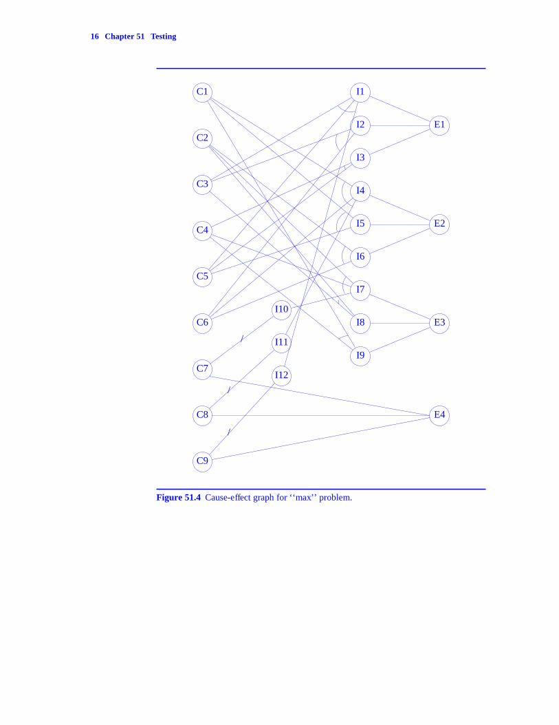
The cause-effect graph for the ‘‘max’’ problem defined above is shown inFigure 51.4. Before examining this graph, we state the following conventions fordrawing cause-effect graphs:

1. Nodes that represent causes are drawn in one column at the left end of thegraph.

2. Nodes that represent effects are drawn in one column at the right end.

3. Intermediate nodes (nodes labeled I1-I12 in Figure 51.4), as needed, aredrawn in between the cause and effect nodes. These are arranged incolumns.

4. Each node (whether cause, intermediate, or effect) can be in one of twostates: true and false. (Later, we shall introduce a third state. For now,these two states will suffice.) For example, a cause node is true iff theBoolean expression it represents is true. In our example, C1 is true iffx < y. An effect node is true iff the effect it denotes does, in fact, occur.Node E3 is true iff the output z is generated by the program.

5. Every edge connects a node in one column to a node in some column to itsright.

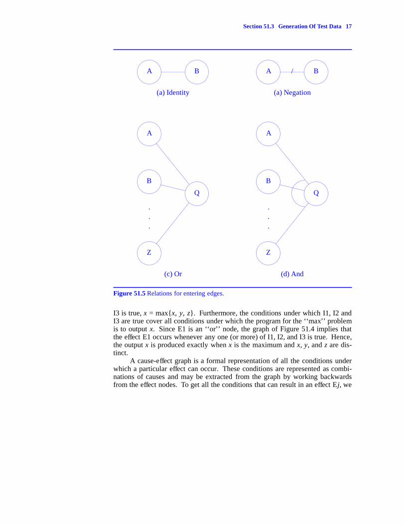
6. The collection of edges that enters any node must be related in exactly oneof the ways shown in Figure 51.5. The ‘‘identity’’ relation expressed byFigure 51.5(a) has the significance that node B is in the same state as nodeA. So, B is true iff A is. The ‘‘negation’’ relation of Figure 51.5(b) meansthat the state of A is different from that of B. If A is true, then B is false. IfA is false, then B is true. The ‘‘or’’ relation of Figure 51.5(c) indicates thatnode Q is true iff at least one of A, B, ..., Z is true. Finally, the ‘‘and’’ rela-tion of Figure 51.5(d) has the property that Q is true iff every one of A, B,..., Z is true.

7. If a single edge comes into a node, then that node is either an identity or anegation node. Node ‘‘B’’ of Figure 51.5(a) is an identity node while node‘‘B’’ of Figure 51.5(b) is a negation node. When all entering edges arerelated by the ‘‘or’’ (‘‘and’’) relation, the node is an ‘‘or’’ (‘‘and’’) node.Node ‘‘Q’’ of Figure 51.5(c) is an ‘‘or’’ node while in Figure 51.5(d), nodeQ is an ‘‘and’’ node.

Returning to our example and Figure 51.4, we see that I1 is true iff C3, C5,and I12 are true. But, I12 is true iff C9 is false. So, I1 is true iff y < x and z < xand y ≠ z. I2 is true iff C3 and C6 are true. I.e., iff y < x and z < y. I3 is true iffC4 and C5 are true. I.e., iff y < z and z < x. Hence, when any one of I1, I2, and

-- --


C1

C2

C3

C4

C5

C6

C7

C8

C9

I1

I2

I3

I4

I5

I6

I7

I8

I9

I10

I11

I12

/

/

/

E1

E2

E3

E4

Figure 51.4 Cause-effect graph for ‘‘max’’ problem.

-- --


A B

(a) Identity

A B/

(a) Negation

A

B

.

.

.

Z

Q

(c) Or

A

B

.

.

.

Z

Q

(d) And

Figure 51.5 Relations for entering edges.

I3 is true, x = max{x, y, z}. Furthermore, the conditions under which I1, I2 andI3 are true cover all conditions under which the program for the ‘‘max’’ problemis to output x. Since E1 is an ‘‘or’’ node, the graph of Figure 51.4 implies thatthe effect E1 occurs whenever any one (or more) of I1, I2, and I3 is true. Hence,the output x is produced exactly when x is the maximum and x, y, and z are dis-tinct.

A cause-effect graph is a formal representation of all the conditions underwhich a particular effect can occur. These conditions are represented as combi-nations of causes and may be extracted from the graph by working backwardsfrom the effect nodes. To get all the conditions that can result in an effect Ej, we

-- --


begin at the node Ej. This node is assigned the state: true. To determine allcombinations of causes that result in a node being in a prespecified state, we usethe following rules:

1. If this is an identity node (Figure 51.5(a)) that is to be in the state true(false), we determine all conditions under which the node on its left is true(false).

2. If this is a negation node that is to be in the state true, we determine allconditions under which the node on its left is false (true).

3. In case this is an ‘‘and’’ node that is to be in the state true, we determinethe conditions under which all the left nodes are true. If the ‘‘and’’ node isto be in the state false, then all combinations of states of the left nodesother than the combination having all left nodes true need to be explored.If there are n left nodes, then there are 2n−1 combinations of states for theleft nodes that will result in the ‘‘and’’ node having the state false. Allcombinations of causes leading to each of these 2n−1 combinations ofstates need to be determined.

4. In the case of an ‘‘or’’ node that is to be in the false state, we determine allconditions under which each of the left nodes is false. In case the ‘‘or’’node is to be in the true state and there are n left nodes, then all cause com-binations that result in any of the 2n−1 combinations of states of the leftnodes that imply the ‘‘or’’ node is in the true state are to be determined.

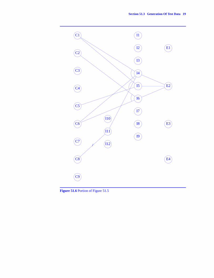
Let us use these rules to determine all conditions under which the effect E2occurs. For clarity, Figure 51.4 has been redrawn in Figure 51.6. Only relevantnodes and edges have been retained.

E2 is an ‘‘or’’ node. Its state is set to true. This node has three left nodes:I4, I5, I6. For E2 to be in the true state, (I4, I5, I6) can be in any one of the sevenstate combinations:

1. (true, true, true)

2. (true, true, false)

3. (true, false, true)

4. (true, false, false)

5. (false, true, true)

6. (false, true, false)

7. (false, false, true)

We need to determine the conditions under which each of the above sevenstate combinations occurs. Let us begin with the first. I4, I5, and I6 are ‘‘and’’nodes. Hence, for I4 to be true, C1, C6, and I11 must be true. Since I11 is anegation node, for I11 to be true, C8 must be false. For I5, C1 and C5 must be

-- --


C1

C2

C3

C4

C5

C6

C7

C8

C9

I1

I2

I3

I4

I5

I6

I7

I8

I9

I10

I11

I12/

E1

E2

E3

E4

Figure 51.6 Portion of Figure 51.5

-- --


true. For I6, C2 and C6 must be true. So, the conditions under which I4, I5, andI6 have the state combination (true, true, true) are:

(C1 and C6 and (not C8)) and (C1 and C5) and (C2 and C6)= C1 and C2 and C5 and C6 and (not C8)

This is the only set of conditions that results in the first of the seven state combi-nations listed above.

It is quite possible to have several sets of conditions that result in a givenstate combination. This, in fact, is the case with the second state combination(true, true, false). There are three possible state combinations of the left nodes,(C2, C6), of I6 that result in I6 having the state false. These are:

1. (true, false)

2. (false, true)

3. (false, false)

These are, respectively, represented by the cause combinations:

1. C2 and (not C6)

2. (not C2) and C6

3. (not C2) and (not C6)

Combining these with the conditions under which I4 and I5 are true, we getthe following three conditions under which (I4, I5, I6) are in the state (true, true,false):

(C1 and C6 and (not C8)) and (C1 and C5) and (C2 and (not C6))(C1 and C6 and (not C8)) and (C1 and C5) and ((not C2) and C6)(C1 and C6 and (not C8)) and (C1 and C5) and ((not C2) and (not C6))

Generalizing from these two examples, we see that there are three differentconditions that lead to the state combination (true, false, true); nine that lead to(true, false, false); seven that lead to (false, true, true); twenty one that lead to(false, true, false); and twenty one that lead to (false, false, true). In all there are65 combinations of input conditions under which E2 can be in the state true.There are 65 for E1, 65 for E3, and 7 for E4. In all there are 202 combinations ofthe causes that result in one of the effects being true!

Some of these combinations may be the same and yet others may be impos-sible. Several combinations are impossible in our example. For instance, thecause combination

C1 and C2 and C5 and C6 and (not C8)

-- --


that results in the state (I4, I5, I6) = (true, true, true) is not possible. This is so asC2 = x < z while C5 = z < x.

Even after the impossible combinations are weeded out and common com-binations combined, the number of cause combinations that remain may be toolarge. In fact, because of the rules used for ‘‘and’’ nodes in the false state andfor ‘‘or’’ nodes in the true state, the number of combinations grows exponen-tially as we move towards the left end of the graph. In an attempt to curb thisexplosive growth in the number of cause combinations that get generated, wesuggest the following strategies:

1. When considering an ‘‘and’’ (‘‘or’’) node that is to be in the false (true)state generate only one of the many cause combinations that results in eachof the 2n−1 state combinations. This avoids further explosive growth in thenumber of generated conditions.

2. When considering an ‘‘and’’ (‘‘or’’) node that is to be in the false (true)state, consider at most n different left node state combinations. Theseshould have the property that each of the left nodes is in the false (true)state in at least one of the state combinations and that no state combinationis an impossible combination. To the extent possible, state combinations inwhich exactly one left node is in the false (true) state are to be preferredover those in which more than one left node is in the false (true) state. Thiscuts down the number of left node state combinations from 2n−1 to at mostn.

To see the difference between these two reduction strategies, consider thecause-effect graph of Figure 51.6. We have already determined that there are 65cause combinations that result in E2 being true. If we use reduction strategy (1),then for each of the seven state combinations that result in E2 being true, weneed to generate only one cause combination. The total number of cause combi-nations to generate is reduced from 65 to 7. If we use strategy (2), then for E2we need to pick at most three state combinations for (I4, I5, I6) that are possible.The guidelines recommend the combinations (true, false, false), (false, true,false), and (false, false, true). Let us consider the first one. For the moment,assume that each of these is possible. The sole cause combination that results inI4 true is:

C1 and C6 and (not C8)

We have seen earlier that there are three state combinations for (C2, C6) thatresult in I6 being false. Under strategy (2), only two of these ((true, false) and(false, true)) need be considered. Similarly, there are two state combinations for(C1, C5) that need to be considered. In all, therefore, we will obtain four sets ofcause conditions that result in (I4, I5, I6) having the state combination (true,false, false). By symmetry, we will obtain four combinations for each of the

-- --


remaining two state combinations under consideration for (I4, I5, I6). Hence, thenumber of generated combinations reduces from 37 to 12.

The four combinations generated for (I4, I5, I6) = (true, false, false) are:

1. (C1 and C6 and (not C8)) and (C1 and (not C5)) and (C2 and (not C6))

2. (C1 and C6 and (not C8)) and (C1 and (not C5)) and ((not C2) and C6)

3. (C1 and C6 and (not C8)) and ((not C1) and C5) and (C2 and (not C6))

4. (C1 and C6 and (not C8)) and ((not C1) and C5) and ((not C2) and C6)

None of these is possible. (1) is not possible as it requires C6 to be bothtrue and false. (3) and (4) are impossible for similar reasons. (2) requires thatboth C2 and C5 be false. But from the definition of C2 and C5, this implies thatC8 be true. This contradicts the requirement in (2) that C8 is false. Since thestate combination (true, false, false) is impossible, we can replace it by someother combination that has I4 = true. An examination of the remaining two statecombinations being considered for (I4, I5, I6) reveals that neither is possible.

So, we need to consider some other state combinations. Since, wheneverI5 or I6 is true, I4 is also true, the only possible combinations are (true, true,false) and (true, false, true). There is only one possible cause combination foreach. These are:

1. (C1 and C6 and (not C8)) and (C1 and C5) and ((not C2) and C6)= C1 and C5 and C6 and (not C2) and (not C8)= C1 and C5 and C6 (by definition of the C’s)

2. (C1 and C6 and (not C8)) and (C1 and (not C5)) and (C2 and C6)= C1 and C2 and C6 and (not C5) and (not C8)= C1 and C2 and C6 (by definition of the C’s)

Similarly, for each of E1 and E3 exactly two cause combinations (whichare not impossible) are generated. For E4, the guidelines for strategy (2) suggestthe following cause combinations (C7, C8, C9): (true, false, false), (false, true,false), and (false, false, true). Each is possible. So, three cause combinations forE4 are generated. Hence, when strategy (2) is used we are left with 9 cause com-binations.

The next step is to determine if these nine cause combinations result in anyeffects in addition to the one noted for each. To do this, we examine the causecombinations one at a time. The truth value of all causes in the combination isascertained. For example, the cause combination for (I4, I5, I6) = (true, true,false) has C1, C5, and C6 true and C2 and C8 false. We begin by assigning thesevalues to the cause nodes C1, C2, C5, C6, and C8. These truth values requirethat C3, C4, C7, and C9 be false. At this time, if there are any causes whosevalue is undetermined, these are assigned the value ‘‘?’’. In our example, nocause has an unassigned truth value. So, no ‘‘?’’’s are introduced.

-- --


Next, we evaluate the states of the remaining nodes by moving left to right.The state of any node depends only on the states of the nodes on its left. So, itsstate may be evaluated using the node type information and the truth values ofthe nodes on its left. The following rules are used to handle the truth value ‘‘?’’:

1. The truth value of an identity or negation node is ‘‘?’’ iff its left node hasvalue ‘‘?’’.

2. The truth value of an ‘‘or’’ node is true iff at least one of its left nodes havevalue true. It is false iff all its left nodes have value false. Otherwise, itsvalue is ‘‘?’’.

3. An ‘‘and’’ node has value true iff all its left nodes have value true. It hasvalue false iff at least one of its left nodes have value false. Otherwise, ithas value ‘‘?’’.

Using these rules, the value of the effect nodes may be determined. For C1,C5, and C6 true and the remaining causes false, we get E1, E3, and E4 false andE2 true.

Let us consider another example. Consider the case E4 = true. Asremarked earlier, when strategy (2) is used, only the following state combina-tions for (C7, C8, C9) are to be considered:

1. (true, false, false)

2. (false, true, false)

3. (false, false, true)

Consider the first of these. This requires C7 to be true and C8 and C9 to be false.When C7 is true, C1 and C3 must be false. The values of C2, C4, C5, and C6 areundetermined and set to ‘‘?’’. Using these truth values, the values of the effectnodes E1-E4 are, respectively, ‘‘?’’, ‘‘?’’, false, and true.

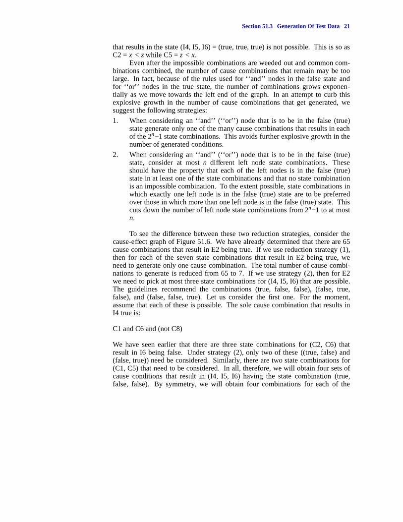
By repeating this process for each of the twelve cause combinations, wecan determine the effects each is expected to produce. This cause-effect relation-ship may be tabulated in the form of a decision table as in Figure 51.7. A deci-sion table has one row for each cause-effect combination. It contains one columnfor each cause and each effect. A ‘‘T’’ entry implies that the correspondingcause or effect is true (or present). An ‘‘F’’ entry implies that it is false (orabsent). A blank entry signifies a value that is trivially determined from theother values and the cause-effect graph. It might evaluate to T, F, or ‘‘?’’.

For the example of Figure 51.4, there are 9 rows in the decision table. Thefirst row of Figure 51.7, for example, states that when the causes C3, C4, and C5are true (i.e., are present), the effect E1 is true. From the definitions of the causesC1-C9 and the specified truth values for C3, C4, and C5, we see that the remain-ing causes must be false. This results in E2, E3, and E4 having the value false.So, all the blanks in first row of the decision table correspond to the value false.For the last row of the table, C7 and C8 are false while C9 and E4 are true. This

-- --


implies that C4 and C6 are false. The values of C1, C2, C3, and C5 are ‘‘?’’.This results in E1 false and E2 and E3 having value ‘‘?’’.

C1 C2 C3 C4 C5 C6 C7 C8 C9 E1 E2 E3 E4

T T T T

T T T T

T T T T

T T T T

T T T T

T T T T

T F F T

F T F T

F F T T

Figure 51.7 Cause-effect decision table for Figure 51.4

Once a decision table has been constructed, it may be reduced using wellknown decision table reduction methods. We shall not go into these here. Theeffect of the reduction is to eliminate rows of the table that are subsumed by oth-ers. Following this reduction, a test set is devised so as to include at least one setof input data for each row of the reduced decision table. Since no row consistsof an impossible set of cause conditions, there is at least one element in the inputdomain that satisfies the cause conditions of each of the rows. Because of thepresence of don’t cares in a decision table, it is possible for one input to satisfythe conditions of more than one row. So, the decision table doesn’t result in astrict partitioning of the input domain. It does, however, come close to this.

From the table of Figure 51.7, we see that our test set for the ‘‘max’’ prob-lem will include at least 9 test data. We need at least one test data for each of thefollowing combination of causes:

1. y < x, y < z, and z < x (eg.: x = 5, y = 3, z = 4)

2. y < x, z < y, and z < x (eg.: x = 5, y = 3, z = 2)

3. x < y, x < z, and z < y (eg.: x = 3, y = 8, z = 4)

4. x < y, z < x, and z < y (eg.: x = 5, y = 7, z = 2)

5. x < y, x < z, and y < z (eg.: x = 1, y = 3, z = 4)

-- --


6. y < x, x < z, and y < z (eg.: x = 2, y = 1, z = 4)

7. x = y, x ≠ z, and y ≠ z (eg.: x = 2, y = 2, z = 6)

8. x ≠ y, x = z, and y ≠ z (eg.: x = 2, y = 5, z = 2)

9. x ≠ y, x ≠ z, and y = z (eg.: x = 2, y = 6, z = 6)

Comparing with the ad hoc I/O partitioning method used in the precedingsection, we see that cause-effect graphing has led to 9 test data rather than 4.

51.3.3 White Box Methods

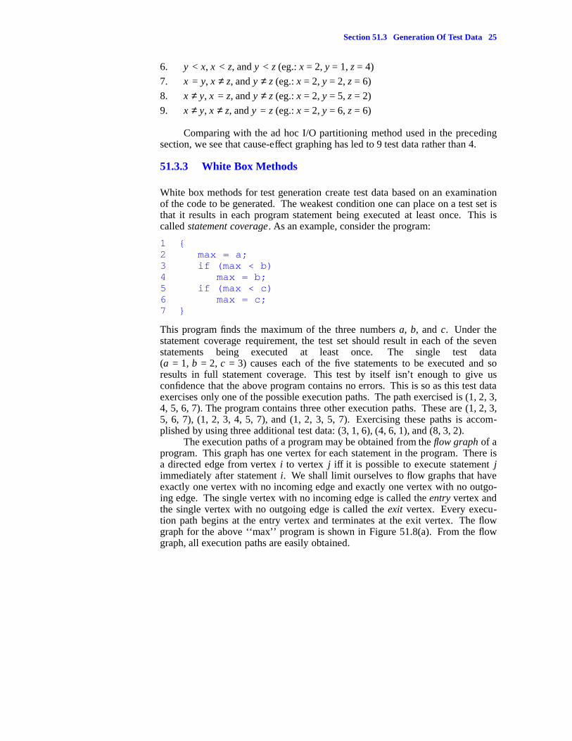
White box methods for test generation create test data based on an examinationof the code to be generated. The weakest condition one can place on a test set isthat it results in each program statement being executed at least once. This iscalled statement coverage. As an example, consider the program:

1 {2 max = a;3 if (max < b)4 max = b;5 if (max < c)6 max = c;7 }

This program finds the maximum of the three numbers a, b, and c. Under thestatement coverage requirement, the test set should result in each of the sevenstatements being executed at least once. The single test data(a = 1, b = 2, c = 3) causes each of the five statements to be executed and soresults in full statement coverage. This test by itself isn’t enough to give usconfidence that the above program contains no errors. This is so as this test dataexercises only one of the possible execution paths. The path exercised is (1, 2, 3,4, 5, 6, 7). The program contains three other execution paths. These are (1, 2, 3,5, 6, 7), (1, 2, 3, 4, 5, 7), and (1, 2, 3, 5, 7). Exercising these paths is accom-plished by using three additional test data: (3, 1, 6), (4, 6, 1), and (8, 3, 2).

The execution paths of a program may be obtained from the flow graph of aprogram. This graph has one vertex for each statement in the program. There isa directed edge from vertex i to vertex j iff it is possible to execute statement jimmediately after statement i. We shall limit ourselves to flow graphs that haveexactly one vertex with no incoming edge and exactly one vertex with no outgo-ing edge. The single vertex with no incoming edge is called the entry vertex andthe single vertex with no outgoing edge is called the exit vertex. Every execu-tion path begins at the entry vertex and terminates at the exit vertex. The flowgraph for the above ‘‘max’’ program is shown in Figure 51.8(a). From the flowgraph, all execution paths are easily obtained.

-- --


1 2 3 4 5 6 7

(a)

1-2 3 4 5 6 7

(b) Reduced Graph

1-3 4 5 6 7

(c) Fully Reduced Graph

Figure 51.8 Flow graphs for max program

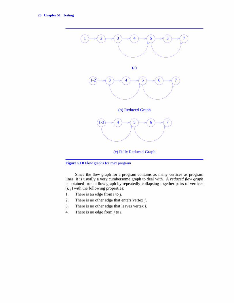
Since the flow graph for a program contains as many vertices as programlines, it is usually a very cumbersome graph to deal with. A reduced flow graphis obtained from a flow graph by repeatedly collapsing together pairs of vertices(i, j) with the following properties:

1. There is an edge from i to j.

2. There is no other edge that enters vertex j.

3. There is no other edge that leaves vertex i.

4. There is no edge from j to i.

-- --


When two vertices i and j are collapsed, the edge from i to j is eliminated.Vertices 1 and 2 of Figure 51.8(a) can be collapsed to get the reduced graph ofFigure 51.8(b). This graph can be reduced further to get the graph of Figure51.8(c). The graph of Figure 51.8(c) cannot be reduced further.

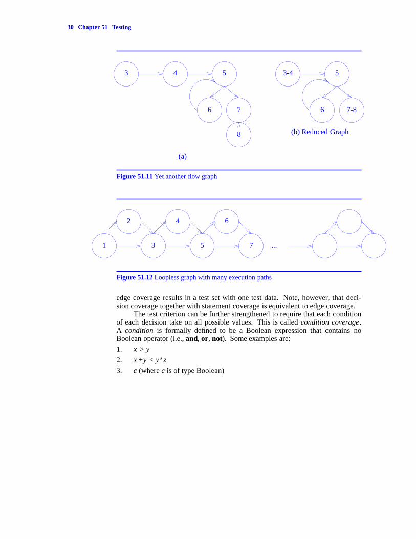
Two hypothetical flow graphs are shown in Figures 51.9(a), 51.10(a), and51.11(a), respectively. The corresponding reduced graphs are shown in Figures51.9(b), 51.10(b), and 51.11(b).

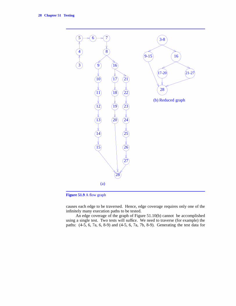
From the reduced flow graph of Figure 51.9(b) we see that the correspond-ing program has three execution paths: (1-8, 9-15, 28), (1-8, 16, 17-20, 28), and(1-8, 16, 21-27, 28). All the execution paths of this program can be tested usingthree test data; one for each of these execution paths. From the reduced flowgraph Figure 51.11(b), we see that there are many execution paths. These aregiven by the expression (3-4, (5, 6)j , 5, 7-8) for j ≥ 0. (5, 6)j is an abbreviationfor 5, 6, 5, 6, ..., 5, 6 where the number of 5’s (and hence of 6’s) is j.

When the number of iterations of a loop is a function of the input size thenumber of execution paths is infinite. Even when we restrict ourselves to pro-grams whose loops are iterated at most 10 or 1000 times, the number of execu-tion paths may be very large. Further, even programs that contain no loops at allmay have a very large number of execution paths. As an example, consider theflow graph of Figure 51.12. There are no loops in the program it represents.However, the number of execution paths is exponential in the number of ver-tices.

While it would be nice to be able to use a test set that exercises each exe-cution path in a program at least once, the size of such a test set will often beinfinite or impractically large. Hence, it is necessary to lower our sights anddevelop criteria for an adequate test set whose coverage is somewhere betweenthe two extremes of total statement coverage and total execution path coverage.

One possibility is to require that each edge of the flow graph be traversedby the test set. This is called edge coverage. Note that if a reduced flow graphhas at least one edge, then traversing all edges of the reduced flow graph resultsin traversing all edges of the full flow graph. If the reduced flow graph has noedges, then the empty test set provides a total edge coverage for the reduced flowgraph but not for the full graph. Note that the full graph has at least one edge asit contains at least the two vertices: entry and exit. Hence, the edge coverage cri-terion may be applied to the reduced graph except in the case that this graph hasno edges.

For the graph of Figure 51.8(c), two sets of test data suffice to obtain edgecoverage. The test data a = 6, b = 2, c = 3 causes the edges (1-3, 5) and (5, 7) tobe traversed. The data a = 1, b = 2, c = 3 causes the edges (1-3, 4), (4, 5), (5, 6),and (6, 7) to be traversed. Only two of the possible four execution paths aretraversed using this test set.

For the graph of Figure 51.9(b), edge coverage requires all execution pathsto be traversed. The edges of Figure 51.11(b) can be covered using a single exe-cution path. In fact, every path of the form (3-4, (5, 6)j , 5, 7-8) for 1 ≤ j ≤ n

-- --


3

4

5 6 7

8

9

10

11

12

13

14

15

16

17

18

19

20

21

22

23

24

25

26

27

28

(a)

3-8

9-15 16

17-20 21-27

28

(b) Reduced graph

Figure 51.9 A flow graph

causes each edge to be traversed. Hence, edge coverage requires only one of theinfinitely many execution paths to be tested.

An edge coverage of the graph of Figure 51.10(b) cannot be accomplishedusing a single test. Two tests will suffice. We need to traverse (for example) thepaths: (4-5, 6, 7a, 6, 8-9) and (4-5, 6, 7a, 7b, 8-9). Generating the test data for

-- --


4 5 6 7a 7b 8 9

(a)

4-5 6 7a 7b 8-9

(b) Reduced Graph

Figure 51.10 Another flow graph

each of these is quite straightforward.The edge coverage criterion requires that all decisions in a program evalu-

ate to both true and false (for two way decisions) during the test.Decision coverage is a criterion that is closely related to edge coverage. In

this criterion, we require that the test set cause each decision to take on all itspossible values (true and false in case of a two way decision). For single entrysingle exit graphs, edge coverage implies decision coverage. However, decisioncoverage may not imply edge coverage. This is, in fact, the case when the flowgraph has no decisions. Decision coverage results in an empty test set whereas

-- --


3 4 5

6 7

8

(a)

3-4 5

6 7-8

(b) Reduced Graph

Figure 51.11 Yet another flow graph

1 3

2

5

4

7

6

...

Figure 51.12 Loopless graph with many execution paths

edge coverage results in a test set with one test data. Note, however, that deci-sion coverage together with statement coverage is equivalent to edge coverage.

The test criterion can be further strengthened to require that each conditionof each decision take on all possible values. This is called condition coverage.A condition is formally defined to be a Boolean expression that contains noBoolean operator (i.e., and, or, not). Some examples are:

1. x > y

2. x +y < y∗z

3. c (where c is of type Boolean)

-- --


Consider the statement:

if ((C1 && C2) || (C3 && C4)) S1;else S2;

where C1, C2, C3, and C4 are conditions and S1 and S2 are statements.Under the edge or decision coverage criteria, we need to use one test set thatcauses (C1 && C2) || (C3 && C4) to be true and another that results inthis decision being false. Condition coverage requires us to use a test set thatcauses each of the four conditions to evaluate to true at least once and to false atleast once. This requires at least two data sets. Some of the possible pairs oftruth value combinations for C1-C4 that satisfy the requirements of conditioncoverage are:

1. (true, true, true, true), (false, false, false, false)

2. (true, false, true, false), (false, true, false, true)

3. (false, false, true, true), (true, true, false, false)

Each of the above requires two data sets. Note that both data sets for (2)result in the decision for the if being false while both data sets for (3) result inthis decision being true. So, a test set that results in condition coverage need notresult in decision coverage.

Note also that there may be no input data that corresponds to any of theabove three pairs of truth value combinations. For example, there may be nodata that results in C1-C4 being true simultaneously. Hence, condition cover-age may require the use of more than two data sets. Two truth value combina-tions for C1-C4 that result in condition coverage and require three data setsare:

1. (true, true, true, true), (true, true, false, false), (false, false, false, true)

2. (true, false, false, true), (true, true, false, true), (false, true, true, false)

Condition coverage can be further strengthened to require that all combina-tions of condition values be tested for. In the above if example, this willrequire the use of 16 test data; one for each truth combination of C1-C4.Several of these combinations may not be possible. So, the number of test datawill generally be smaller.

Of the test coverage criteria we have discussed so far, execution path cov-erage is generally the most demanding. A test set that results in total executionpath coverage also results in statement and decision coverage. It may, however,not result in condition coverage. Total execution path coverage often requires aninfinite number of test data or at least a prohibitively large number of test data.Hence, total path coverage is often impossible in practice.

-- --


It is often possible to use a test set that satisfies all three of the following:

1. statement coverage

2. decision coverage

3. all combinations condition coverage

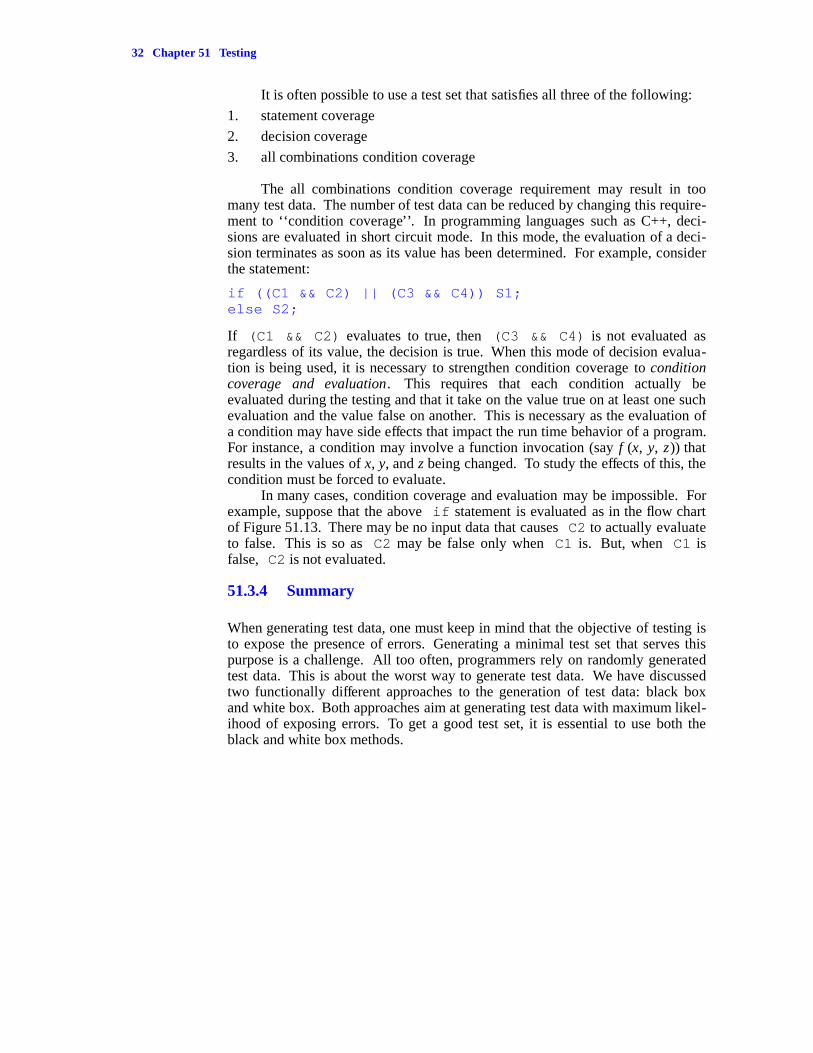
The all combinations condition coverage requirement may result in toomany test data. The number of test data can be reduced by changing this require-ment to ‘‘condition coverage’’. In programming languages such as C++, deci-sions are evaluated in short circuit mode. In this mode, the evaluation of a deci-sion terminates as soon as its value has been determined. For example, considerthe statement:

if ((C1 && C2) || (C3 && C4)) S1;else S2;

If (C1 && C2) evaluates to true, then (C3 && C4) is not evaluated asregardless of its value, the decision is true. When this mode of decision evalua-tion is being used, it is necessary to strengthen condition coverage to conditioncoverage and evaluation. This requires that each condition actually beevaluated during the testing and that it take on the value true on at least one suchevaluation and the value false on another. This is necessary as the evaluation ofa condition may have side effects that impact the run time behavior of a program.For instance, a condition may involve a function invocation (say f (x, y, z)) thatresults in the values of x, y, and z being changed. To study the effects of this, thecondition must be forced to evaluate.

In many cases, condition coverage and evaluation may be impossible. Forexample, suppose that the above if statement is evaluated as in the flow chartof Figure 51.13. There may be no input data that causes C2 to actually evaluateto false. This is so as C2 may be false only when C1 is. But, when C1 isfalse, C2 is not evaluated.

51.3.4 Summary

When generating test data, one must keep in mind that the objective of testing isto expose the presence of errors. Generating a minimal test set that serves thispurpose is a challenge. All too often, programmers rely on randomly generatedtest data. This is about the worst way to generate test data. We have discussedtwo functionally different approaches to the generation of test data: black boxand white box. Both approaches aim at generating test data with maximum likel-ihood of exposing errors. To get a good test set, it is essential to use both theblack and white box methods.

-- --


C1 false C3 false S2

C2

S1

C4

true

true

false

true

true false

Figure 51.13 Flow chart for short circuit evaluation

Test data obtained from black box methods can expose errors resultingfrom missing code segments, boundary conditions, numerical errors, interestingcombinations of input conditions, etc. Test data obtained from white boxmethods may not detect such errors.

Test data obtained from white box methods will expose errors resultingfrom uninitialized variables, misspelled variable names, incorrect conditions (forexample x < y instead of y < x), unreachable code segments, etc. These errorsmay not be detected by the black box data.

The black and white box methods provide guidelines for a minimum testset. In practice, it may be possible to use more than a minimum test set. In thiscase, it is desirable to use additional tests in some uniform way. We would liketo exercise all code segments uniformly. To accomplish this, one may useautomatic program instrumentation aids. These aids provide statistics on the fre-quency of execution of each statement or flow graph edge. They can also recordthe number of times each decision took on a certain value, the number of timeseach condition had a certain evaluation, etc. Based on this information, one candevise additional tests to exercise those parts of the program that have not beensufficiently exercised. The interested reader is referred to the paper on program

-- --


instrumentation by J. Huang that is cited in the references section of this chapter.Program instrumentation is also useful in obtaining a test set that satisfies

certain criteria. After a few test data have been used, the results from the pro-gram instrumentation can be used to determine what needs to be done to meetthe test criteria. Additional test data to meet this end can now be obtained.EXERCISES

5. List all the conditions under which (I4, I5, and I6) take on each of the fol-lowing state combinations. See Figure 51.4. For each set of conditionsdetermine whether it is an impossible condition.

a. (true, false, true)

b. (true, false, false)

c. (false, true, true)

d. (false, true, false)

e. (false, false, true)

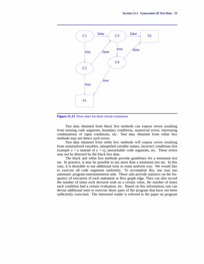
6. For the cause-effect graph of Figure 51.14, obtain all cause combinationsthat result in each of the effects E1, E2, and E3. Present these in a decisiontable in which each different cause combination is represented by a singlerow. For each set of cause combinations, all effects should be marked T, F,or ‘‘?’’.

C1 I1 E1

C2 I2 E2

C3 I3 E3

C4

Figure 51.14

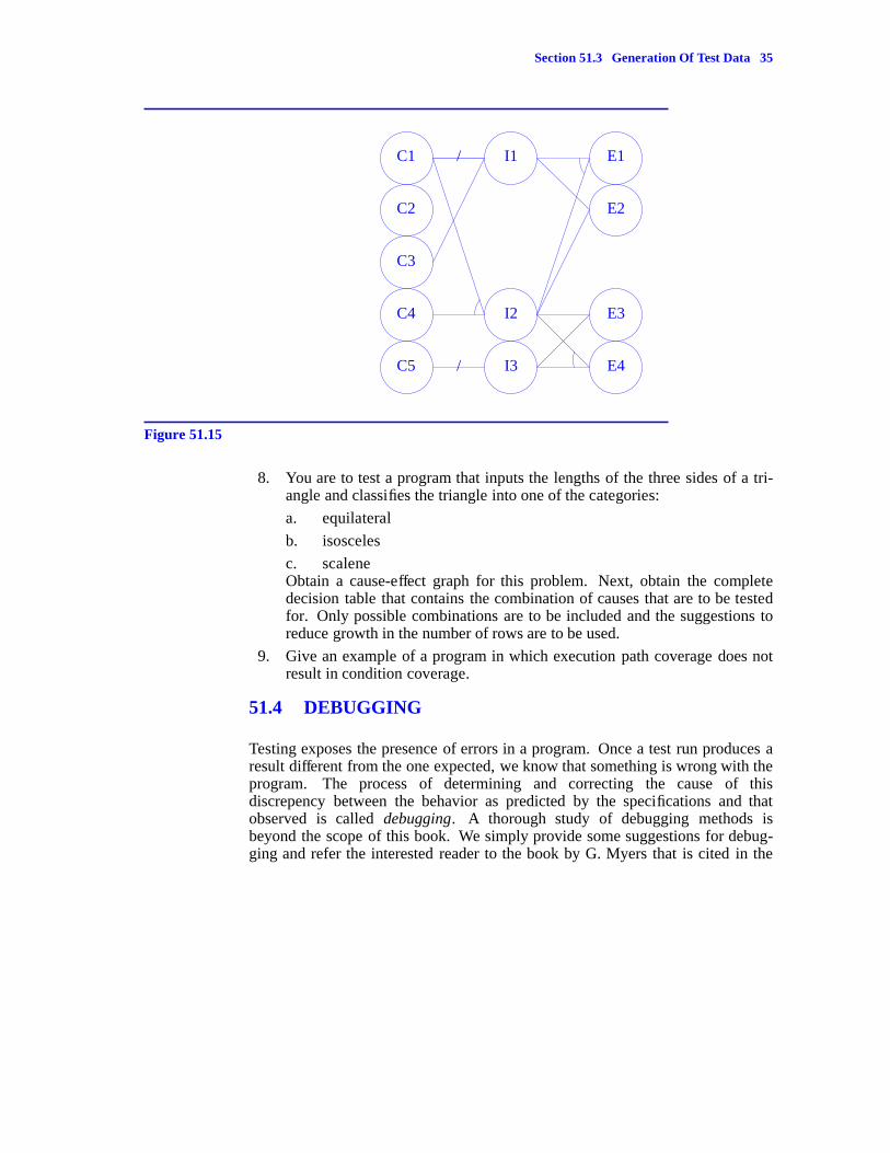
7. Do the previous exercise for the cause-effect graph of Figure 51.15.

-- --


C1 / I1 E1

C2

C3

E2

C4 I2 E3

C5 / I3 E4

Figure 51.15

8. You are to test a program that inputs the lengths of the three sides of a tri-angle and classifies the triangle into one of the categories:

a. equilateral

b. isosceles

c. scaleneObtain a cause-effect graph for this problem. Next, obtain the completedecision table that contains the combination of causes that are to be testedfor. Only possible combinations are to be included and the suggestions toreduce growth in the number of rows are to be used.

9. Give an example of a program in which execution path coverage does notresult in condition coverage.

51.4 DEBUGGING

Testing exposes the presence of errors in a program. Once a test run produces aresult different from the one expected, we know that something is wrong with theprogram. The process of determining and correcting the cause of thisdiscrepency between the behavior as predicted by the specifications and thatobserved is called debugging. A thorough study of debugging methods isbeyond the scope of this book. We simply provide some suggestions for debug-ging and refer the interested reader to the book by G. Myers that is cited in the

-- --


references section.

1. Use incremental testing so that the cause of the error is localized.

2. Try to determine the cause of an error by logical reasoning. If this fails,then you may wish to perform a program trace to determine when the pro-gram started performing incorrectly. This becomes infeasible when theprogram executes many instructions with that test data. The program traceis too long to be examined manually. When this happens, testing must berefined to isolate the part of the code that is suspect and a trace of this partobtained.

3. Do not attempt to correct errors by creating exceptions. Soon, the numberof exceptions will be very large. Errors should be corrected by first deter-mining their cause and then redesigning your solution as necessary.

4. When correcting an error, be certain that your correction does not result inerrors where there were none before. Run your corrected program on thetest data on which it worked alright before to be sure that it still workscorrectly on this data.

51.5 REFERENCES AND SELECTED READINGS

The text: The art of software testing, by G. Myers, John Wiley, New York, 1979contains many do’s and don’ts of program testing and debugging. It also con-tains chapters on walk-throughs, test design, and test generation tools. The ter-minology ‘‘big bang’’ is borrowed from this book.

The following papers discuss methods to generate test sets: Validation,verification, and testing of computer software, by W. R. Adrions, M. Branstad,and J. Cherniavsky, ACM Computing Surveys, Vol. 14, No. 2, June 1982, pp.159-192; Static analysis and dynamic testing of computer software, by R. Fair-ley, IEEE Computer, April 1978, pp. 14-23; Hints on test data selection: Helpfulfor the practicing programmer, by R. DeMillo, R. Lipton, and F. Sayward, IEEEComputer, April 1978, pp. 34-41; and Program instrumentation and softwaretesting, by J. Huang, IEEE Computer, April 1978, pp. 25-32.

A system that generates test data and several references to other such sys-tems can be found in the paper: A system to generate test data and symbolicallyexecute programs, by L. Clarke, IEEE Trans. On Software Engineering, Sept.1976, pp. 215-222.

-- --

CHAPTER 51 TESTING - cise.ufl.edu

Documents

Transcript of CHAPTER 51 TESTING - cise.ufl.edu