Chapter 5 Ratio and Product Methods of...
23
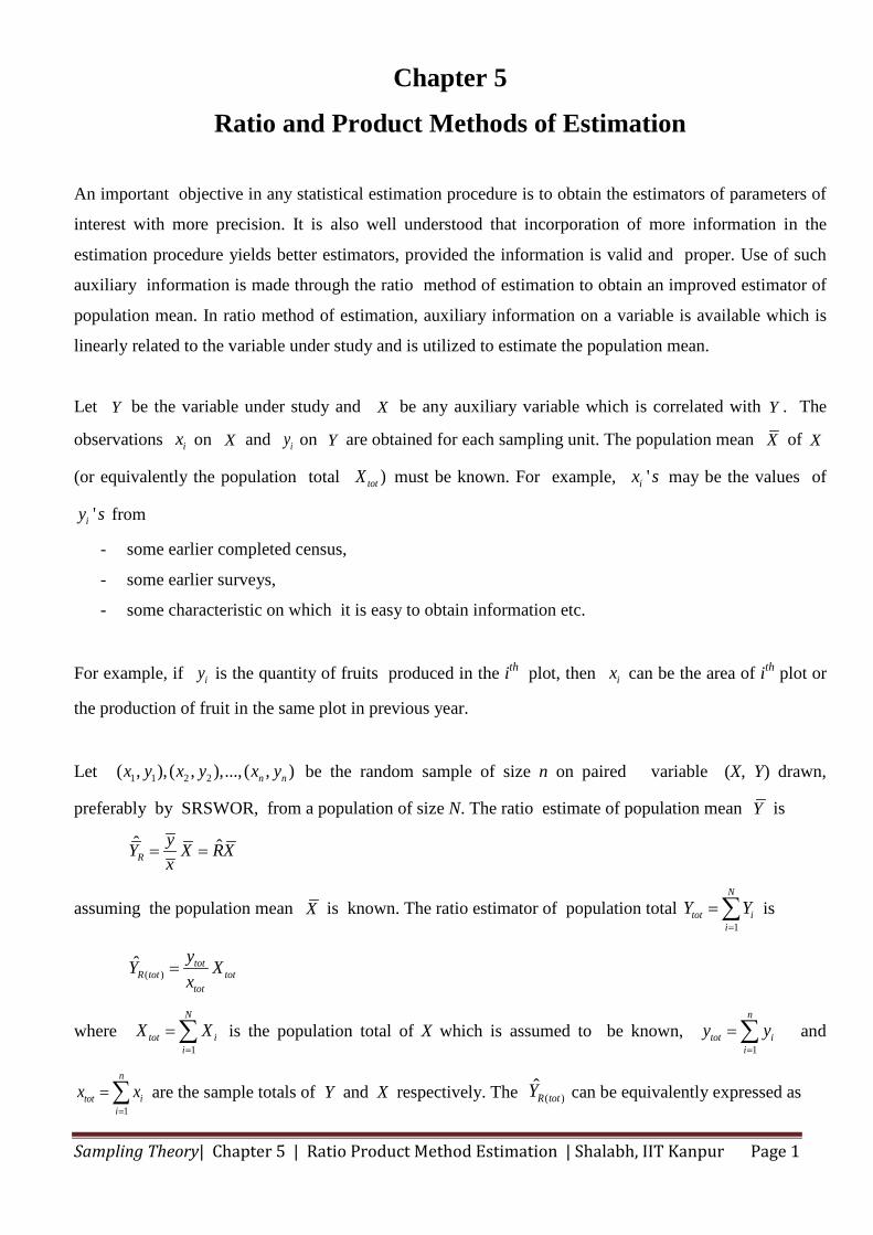
Sampling Theory| Chapter 5 | Ratio Product Method Estimation | Shalabh, IIT Kanpur Page 1 Chapter 5 Ratio and Product Methods of Estimation An important objective in any statistical estimation procedure is to obtain the estimators of parameters of interest with more precision. It is also well understood that incorporation of more information in the estimation procedure yields better estimators, provided the information is valid and proper. Use of such auxiliary information is made through the ratio method of estimation to obtain an improved estimator of population mean. In ratio method of estimation, auxiliary information on a variable is available which is linearly related to the variable under study and is utilized to estimate the population mean. Let Y be the variable under study and X be any auxiliary variable which is correlated with Y . The observations i x on X and i y on Y are obtained for each sampling unit. The population mean X of X (or equivalently the population total ) tot X must be known. For example, ' i x s may be the values of ' i y s from - some earlier completed census, - some earlier surveys, - some characteristic on which it is easy to obtain information etc. For example, if i y is the quantity of fruits produced in the i th plot, then i x can be the area of i th plot or the production of fruit in the same plot in previous year. Let 1 1 2 2 ( , ),( , ),...,( , ) n n x y x y x y be the random sample of size n on paired variable (X, Y) drawn, preferably by SRSWOR, from a population of size N. The ratio estimate of population mean Y is ˆ ˆ R y Y X RX x = = assuming the population mean X is known. The ratio estimator of population total 1 N tot i i Y Y = = ∑ is ( ) ˆ tot R tot tot tot y Y X x = where 1 N tot i i X X = = ∑ is the population total of X which is assumed to be known, 1 n tot i i y y = = ∑ and 1 n tot i i x x = = ∑ are the sample totals of Y and X respectively. The ( ) ˆ R tot Y can be equivalently expressed as
Transcript of Chapter 5 Ratio and Product Methods of...
Sampling Theory| Chapter 5 | Ratio Product Method Estimation | Shalabh, IIT Kanpur Page 1
Chapter 5
Ratio and Product Methods of Estimation
An important objective in any statistical estimation procedure is to obtain the estimators of parameters of
interest with more precision. It is also well understood that incorporation of more information in the
estimation procedure yields better estimators, provided the information is valid and proper. Use of such
auxiliary information is made through the ratio method of estimation to obtain an improved estimator of
population mean. In ratio method of estimation, auxiliary information on a variable is available which is
linearly related to the variable under study and is utilized to estimate the population mean.
Let Y be the variable under study and X be any auxiliary variable which is correlated with Y . The
observations ix on X and iy on Y are obtained for each sampling unit. The population mean X of X
(or equivalently the population total )totX must be known. For example, 'ix s may be the values of
'iy s from
- some earlier completed census,
- some earlier surveys,
- some characteristic on which it is easy to obtain information etc.
For example, if iy is the quantity of fruits produced in the ith plot, then ix can be the area of ith plot or
the production of fruit in the same plot in previous year.
Let 1 1 2 2( , ), ( , ),..., ( , )n nx y x y x y be the random sample of size n on paired variable (X, Y) drawn,
preferably by SRSWOR, from a population of size N. The ratio estimate of population mean Y is
ˆ ˆR
yY X RXx
= =
assuming the population mean X is known. The ratio estimator of population total 1
N
tot ii
Y Y=
=∑ is
( )ˆ totR tot tot
tot
yY Xx
=
where 1
N
tot ii
X X=
=∑ is the population total of X which is assumed to be known, 1
n
tot ii
y y=
=∑ and
1
n
tot ii
x x=
=∑ are the sample totals of Y and X respectively. The ( )R totY can be equivalently expressed as
Sampling Theory| Chapter 5 | Ratio Product Method Estimation | Shalabh, IIT Kanpur Page 2
( )ˆ
ˆ .
R tot tot
tot
yY XxRX
=
=
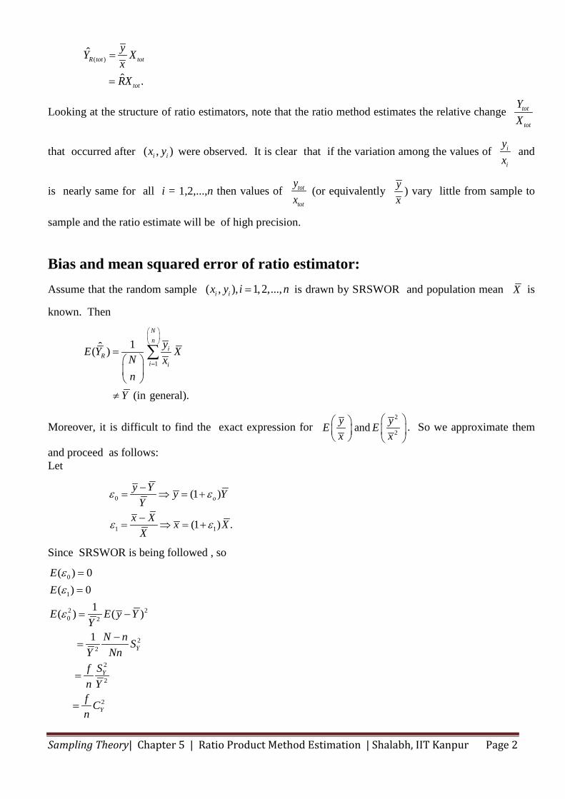
Looking at the structure of ratio estimators, note that the ratio method estimates the relative change tot
tot
YX
that occurred after ( , )i ix y were observed. It is clear that if the variation among the values of i
i
yx
and
is nearly same for all i = 1,2,...,n then values of tot
tot
yx
(or equivalently yx
) vary little from sample to
sample and the ratio estimate will be of high precision.
Bias and mean squared error of ratio estimator: Assume that the random sample ( , ), 1, 2,...,i ix y i n= is drawn by SRSWOR and population mean X is
known. Then
1
1ˆ( )
(in general).
Nn
iR
i i
yE Y XN xn
Y
=
=
≠
∑
Moreover, it is difficult to find the exact expression for 2
2andy yE Ex x
. So we approximate them
and proceed as follows: Let
0
1 1
(1 )
(1 ) .
oy Y Y
Yx X x X
X
yε ε
ε ε
−= ⇒ = +
−= ⇒ = +
Since SRSWOR is being followed , so
0
1
2 20 2
22
2
2
2
( ) 0( ) 0
1( ) ( )
1Y
Y
Y
EE
E E YY
N n SY Nn
Sfn Yf Cn
y
εε
ε
==
= −
−=
=
=
Sampling Theory| Chapter 5 | Ratio Product Method Estimation | Shalabh, IIT Kanpur Page 3
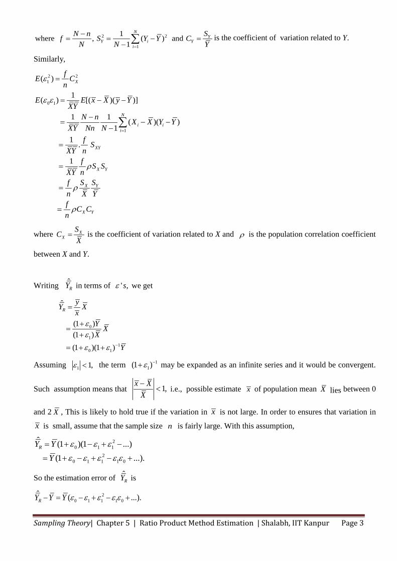
2 2
1
1where , ( ) and1
NY
Y i Yi
SN nf S Y Y CN N Y=
−= = − =
− ∑ is the coefficient of variation related to Y.
Similarly,
2 21
0 1
1
( )
1( ) [( )( )]
1 1 ( )( )1
1 .
1
X
N
i ii
XY
X Y
X Y
X Y
fE Cn
E E x X y YXY
N n X X Y YXY Nn N
f SXY n
f S SXY n
S Sfn X Yf C Cn
ε
ε ε
ρ
ρ
ρ
=
=
= − −
−= − −
−
=
=
=
=
∑
where XX
SCX
= is the coefficient of variation related to X and ρ is the population correlation coefficient
between X and Y.
Writing ˆRY in terms of ' ,sε we get
0
11
0 1
ˆ
(1 )(1 )(1 )(1 )
RyY Xx
Y XX
Y
εε
ε ε −
=
+=
+
= + +
Assuming 1 1,ε < the term 11(1 )ε −+ may be expanded as an infinite series and it would be convergent.
Such assumption means that 1,x XX−
< i.e., possible estimate x of population mean X lies between 0
and 2 X , This is likely to hold true if the variation in x is not large. In order to ensures that variation in
x is small, assume that the sample size n is fairly large. With this assumption,
20 1 1
20 1 1 1 0
ˆ (1 )(1 ...)(1 ...).
RY YY
ε ε ε
ε ε ε ε ε
= + − + −
= + − + − +
So the estimation error of ˆRY is
20 1 1 1 0
ˆ ( ...).RY Y Y ε ε ε ε ε− = − + − +
Sampling Theory| Chapter 5 | Ratio Product Method Estimation | Shalabh, IIT Kanpur Page 4
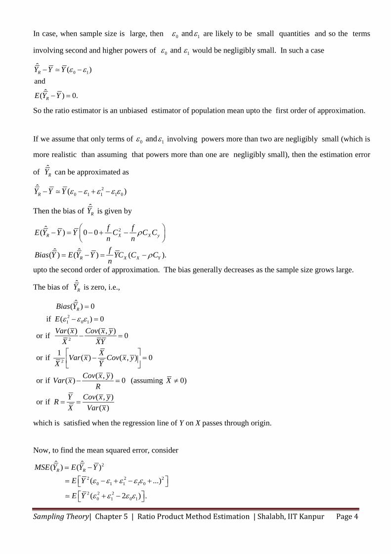
In case, when sample size is large, then 0 1andε ε are likely to be small quantities and so the terms
involving second and higher powers of 0 1andε ε would be negligibly small. In such a case
0 1ˆ ( )and
ˆ( ) 0.
R
R
Y Y Y
E Y Y
ε ε− −
− =
So the ratio estimator is an unbiased estimator of population mean upto the first order of approximation.
If we assume that only terms of 0 1andε ε involving powers more than two are negligibly small (which is
more realistic than assuming that powers more than one are negligibly small), then the estimation error
of ˆRY can be approximated as
20 1 1 1 0
ˆ ( )RY Y Y ε ε ε ε ε− − + −
Then the bias of ˆRY is given by
2ˆ( ) 0 0
ˆ ˆ( ) ( ) ( ).
R X X y
R X X Y
f fE Y Y Y C C Cn nfBias Y E Y Y YC C Cn
ρ
ρ
− = − + −
= − = −
upto the second order of approximation. The bias generally decreases as the sample size grows large.
The bias of ˆRY is zero, i.e.,
21 0 1
2
2
ˆ ( ) 0 if ( ) 0
( ) ( , )or if 0
1or if ( ) ( , ) 0
( , )or if ( ) 0 (assuming 0)
( , )or if( )
RBias YEVar x Cov x y
X XYXVar x Cov x y
X YCov x yVar x X
RY Cov x yRX Var x
ε ε ε
=
− =
− =
− =
− = ≠
= =
which is satisfied when the regression line of Y on X passes through origin.
Now, to find the mean squared error, consider
2
2 2 20 1 1 1 0
2 2 20 1 0 1
ˆ ˆ( ) ( )
( ...)
( 2 ) .
R RMSE Y E Y Y
E Y
E Y
ε ε ε ε ε
ε ε ε ε
= −
= − + − + + −
Sampling Theory| Chapter 5 | Ratio Product Method Estimation | Shalabh, IIT Kanpur Page 5
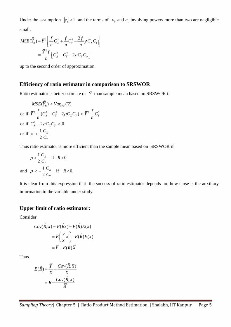
Under the assumption 1 1ε < and the terms of 0 1andε ε involving powers more than two are negligible
small,
2 2 2
22 2
2ˆ( )
2
R X Y X Y
X Y X y
f f fMSE Y Y C C C Cn n n
Y f C C C Cn
ρ
ρ
= + −
= + −
up to the second order of approximation.
Efficiency of ratio estimator in comparison to SRSWOR
Ratio estimator is better estimate of Y than sample mean based on SRSWOR if
2 2 2 2 2
2
ˆ ( ) ( )
or if ( 2 )
or if 2 01or if .2
R SRS
X Y X Y Y
X X Y
X
Y
MSE Y Var yf fY C C C C Y Cn n
C C CCC
ρ
ρ
ρ
<
+ − <
− <
>
Thus ratio estimator is more efficient than the sample mean based on SRSWOR if
1 if 02
1and if 0.2
X
Y
X
Y
C RC
C RC
ρ
ρ
> >
< − <
It is clear from this expression that the success of ratio estimator depends on how close is the auxiliary
information to the variable under study.
Upper limit of ratio estimator: Consider
ˆ ˆ ˆ( , ) ( ) ( ) ( )
ˆ( ) ( )
ˆ( ) .
Cov R x E Rx E R E xyE x E R E xx
Y E R X
= −
= −
= −
Thus
ˆ( , )ˆ( )
ˆ( , )
Y Cov R xE RX X
Cov R xRX
= −
= −

Sampling Theory| Chapter 5 | Ratio Product Method Estimation | Shalabh, IIT Kanpur Page 6
ˆ ˆ,
ˆ ˆ( ) ( )ˆ( , )
xR x R
Bias R E R R
Cov R xX
Xρ σ σ
= −
= −
= −
where ˆ ,R xρ is the correlation between ˆˆ and ; and xRR x σ σ are the standard errors of ˆ andR x
respectively.
Thus
( )
ˆ ˆ,
ˆˆ ,
ˆ( )
1 .
xR x R
xRR x
Bias RX
X
ρ σ σ
σ σρ
−=
≤ ≤
assuming 0.X > Thus
ˆ
ˆ
ˆ( )
ˆ( )or
x
R
XR
Bias RX
Bias R C
σσ
σ
≤
≤
where XC is the coefficient of variation of X. If XC < 0.1, then the bias in R may be safely regarded
as negligible in relation to standard error of ˆ.R
Alternative form of MSE ˆ( )RY
Consider 2
2
1 12
1
2 2 2
1 1 1
2 2 2 2
1
( ) ( ) ( )
( ) ( ) (Using )
( ) ( ) 2 ( )( )
1 ( ) 2 .1
N N
i i i ii i
N
i ii
N N N
i i i ii i i
N
i i Y X XYi
Y RX Y Y Y RX
Y Y R X X Y RX
Y Y R X X R X X Y Y
Y RX S R S RSN
= =
=
= = =
=
− = − + −
= − + − =
= − + − − − −
− = + −−
∑ ∑
∑
∑ ∑ ∑
∑
The MSE of ˆRY has already been derived which is now expressed again as follows:
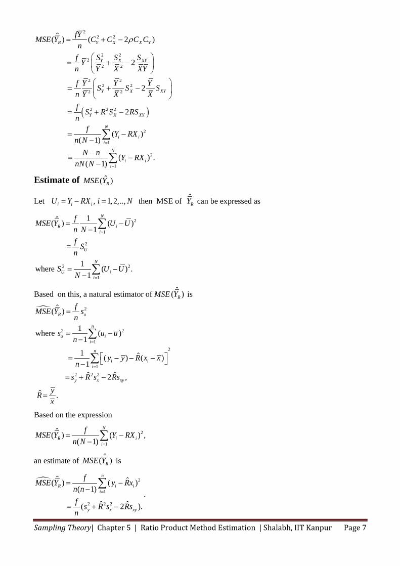
Sampling Theory| Chapter 5 | Ratio Product Method Estimation | Shalabh, IIT Kanpur Page 7
( )
22 2
2 22
2 2
2 22 2
2 2
2 2 2
2
1
2
1
ˆ( ) ( 2 )
2
2
2
( )( 1)
( ) .( 1)
R Y X X Y
Y X XY
Y X XY
Y X XY
N
i ii
N
i ii
fYMSE Y C C C Cn
S S Sf Yn Y X XY
f Y Y YS S Sn Y X Xf S R S RSn
f Y RXn N
N n Y RXnN N
ρ
=
=
= + −
= + −
= + −
= + −
= −−
−= −
−
∑
∑
Estimate of ˆ( )RMSE Y
Let , 1, 2,..,i i iU Y RX i N= − = then MSE of ˆRY can be expressed as
2
1
2
2 2
1
1ˆ( ) ( )1
=
1where ( ) .1
N
R ii
U
N
U ii
fMSE Y U Un Nf Sn
S U UN
=
=
= −−
= −−
∑
∑
Based on this, a natural estimator of MSE ˆ( )RY is
2
2 2
12
1
2 2 2
ˆ( )
1where ( )1
1 ˆ( ) ( )1ˆ ˆ2 ,
ˆ .
R u
n
u ii
n
i ii
y x xy
fMSE Y sn
s u un
y y R x xn
s R s RsyRx
=
=
=
= −−
= − − − −
= + −
=
∑
∑
Based on the expression
2
1
ˆ( ) ( ) ,( 1)
N
R i ii
fMSE Y Y RXn N =
= −− ∑
an estimate of ˆ( )RMSE Y is
2
1
2 2 2
ˆ ˆ( ) ( )( 1)
ˆ ˆ( 2 ).
n
R i ii
y x xy
fMSE Y y Rxn nf s R s Rsn
=
= −−
= + −
∑.
Sampling Theory| Chapter 5 | Ratio Product Method Estimation | Shalabh, IIT Kanpur Page 8
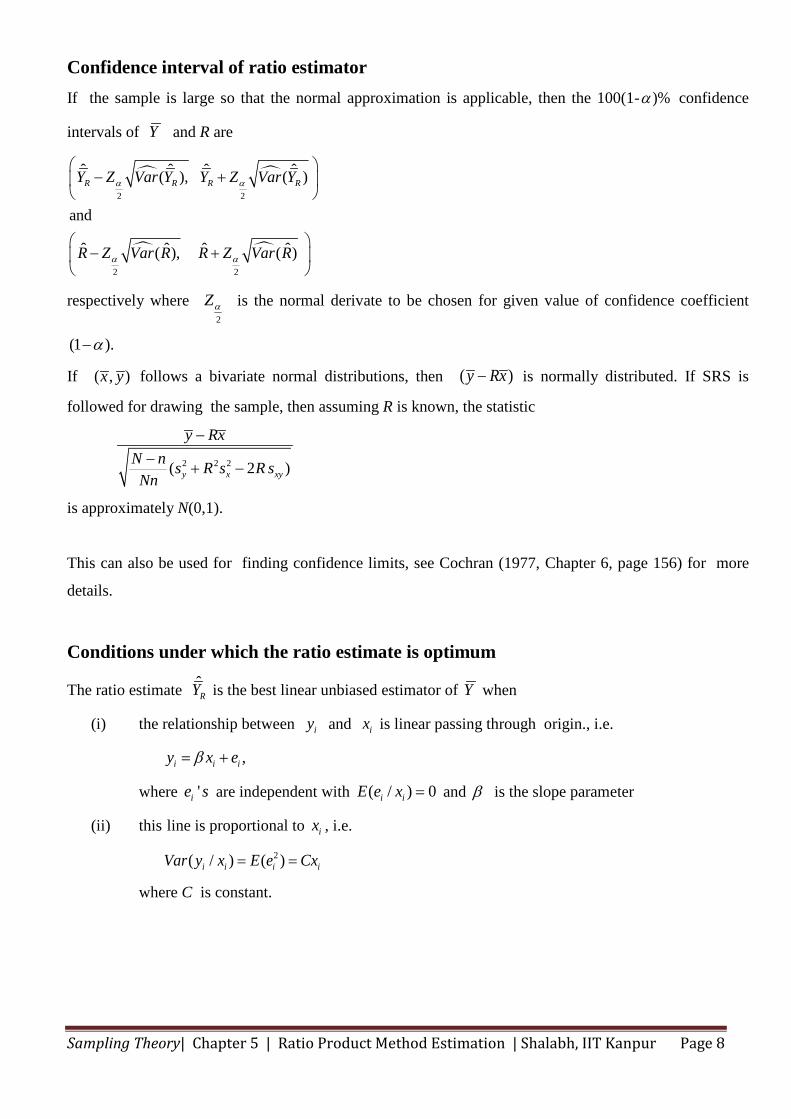
Confidence interval of ratio estimator If the sample is large so that the normal approximation is applicable, then the 100(1- )%α confidence
intervals of Y and R are
2 2
2 2
ˆ ˆ ˆ ˆ( ), ( )
and
ˆ ˆ ˆ ˆ( ), ( )
R R R RY Z Var Y Y Z Var Y
R Z Var R R Z Var R
α α
α α
− +
− +
respectively where 2
Zα is the normal derivate to be chosen for given value of confidence coefficient
(1 ).α−
If ( , )x y follows a bivariate normal distributions, then ( )y Rx− is normally distributed. If SRS is
followed for drawing the sample, then assuming R is known, the statistic
2 2 2( 2 )y x xy
y RxN n s R s R sNn
−−
+ −
is approximately N(0,1).
This can also be used for finding confidence limits, see Cochran (1977, Chapter 6, page 156) for more
details.
Conditions under which the ratio estimate is optimum
The ratio estimate ˆRY is the best linear unbiased estimator of Y when
(i) the relationship between iy and ix is linear passing through origin., i.e.
,i i iy x eβ= +
where 'ie s are independent with ( / ) 0i iE e x = and β is the slope parameter
(ii) this line is proportional to ix , i.e.
2( / ) ( )i i i iVar y x E e Cx= =
where C is constant.

Sampling Theory| Chapter 5 | Ratio Product Method Estimation | Shalabh, IIT Kanpur Page 9
Proof. Consider the linear estimate of β because 1
ˆn
i ii
yβ=
=∑where i i iy x eβ= + and i ‘s are constant.
Then β is unbiased if Y Xβ= as ( ) ( / ).i iE y X E e xβ= +
If n sample values of ix are kept fixed and then in repeated sampling
1
2 2
1 1
ˆ ( )
ˆand ( ) ( / )
n
i ii
n n
i i i i ii i
E x
Var Var y x C x
β β
β
=
= =
=
= =
∑
∑ ∑
So 1
ˆ( ) when 1.n
i ii
E xβ β=
= =∑
Consider the minimization of ( / )i iVar y x subject to the condition for being the unbiased estimator
11
n
i ii
x=
=∑ using Lagrangian function. Thus the Lagrangian function with Lagrangian multiplier is
1
21
1 1
1
1
1
( / ) 2 ( 1.)
2 ( 1).
Now
0 , 1,2,..,
0 1
Using 1
or 1
1or .
n
i i i ii
n n
i i ii i
i i ii
n
i ii
n
i ii
n
ii
Var y x x
C x x
x x i n
x
x
x
nx
ϕ λ
λ
ϕ λ
ϕλ
λ
λ
=
= =
=
=
=
= − −
= − −
∂= ⇒ = =
∂
∂= ⇒ =
∂
=
=
=
∑
∑ ∑
∑
∑
∑
Thus
1i nx=
and so 1ˆ .
n
ii
yy
nx xβ == =
∑
Thus β is not only superior to y but also the best in the class of linear and unbiased estimators.
Sampling Theory| Chapter 5 | Ratio Product Method Estimation | Shalabh, IIT Kanpur Page 10
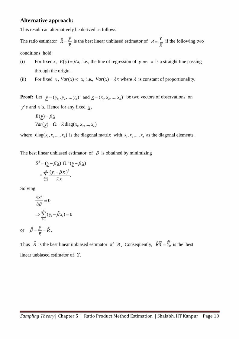
Alternative approach: This result can alternatively be derived as follows:
The ratio estimator ˆ yRx
= is the best linear unbiased estimator of YRX
= if the following two
conditions hold:
(i) For fixed , ( ) ,x E y xβ= i.e., the line of regression of ony x is a straight line passing
through the origin.
(ii) For fixed x , ( ) , i.e., ( ) whereVar x x Var x xλ λ∝ = is constant of proportionality.
Proof: Let 1) 2 1 2( , ,..., ) ' and ( , ,..., ) 'n ny y y y x x x x= = be two vectors of observations on
' and ' .y s x s Hence for any fixed x ,
1 2
( )
( ) diag( , ,..., )n
E y x
Var y x x x
β
λ
=
= Ω =
where 1 2diag( , ,..., )nx x x is the diagonal matrix with 1 2, ,..., nx x x as the diagonal elements.
The best linear unbiased estimator of β is obtained by minimizing
2 1
2
1
( ) ' ( )
( ) .n
i i
i i
S y x y x
y xx
β β
βλ
−
=
= − Ω −
−=∑
Solving
2
1
0
ˆ( ) 0n
i ii
S
y x
β
β=
∂=
∂
⇒ − =∑
or ˆ ˆy Rx
β = = .
Thus R is the best linear unbiased estimator of R . Consequently, ˆˆRRX Y= is the best
linear unbiased estimator of .Y
Sampling Theory| Chapter 5 | Ratio Product Method Estimation | Shalabh, IIT Kanpur Page 11
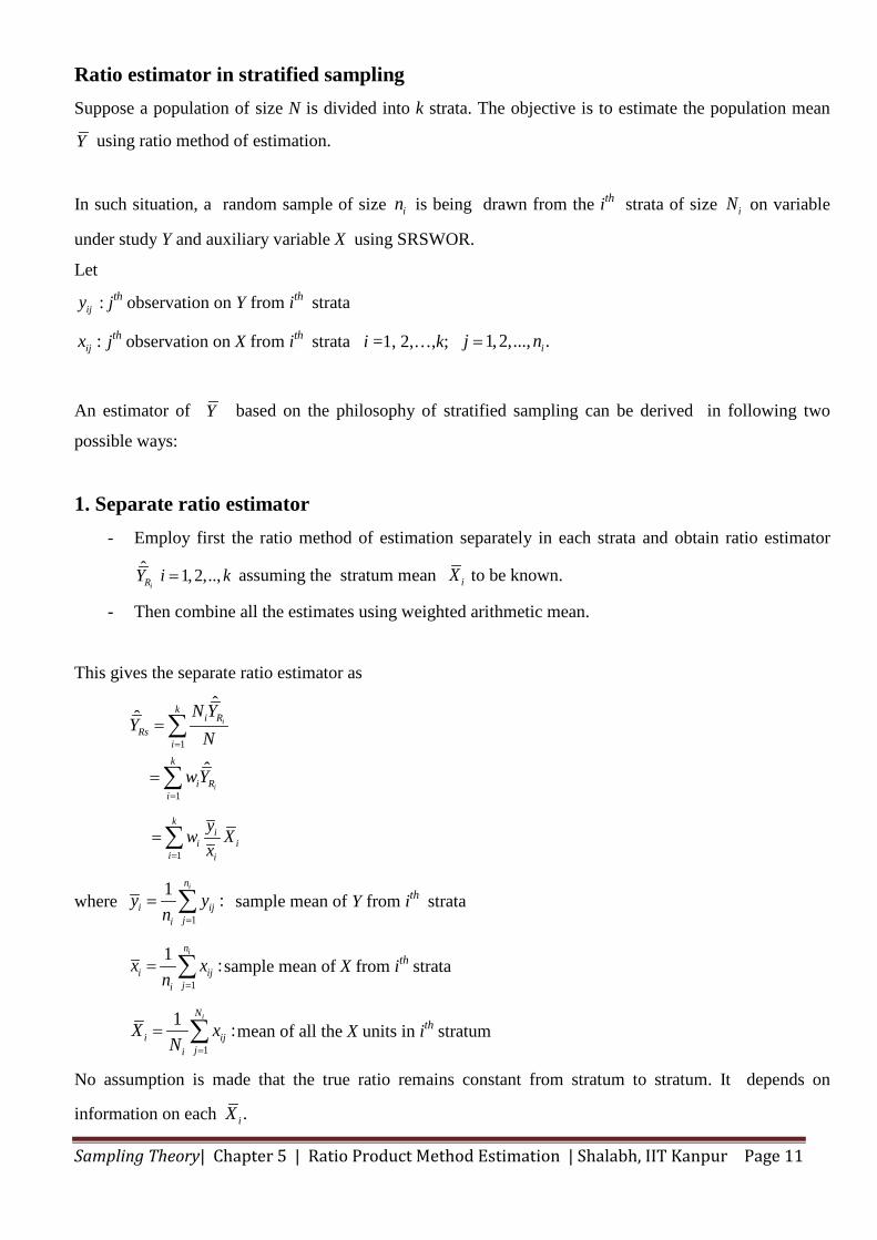
Ratio estimator in stratified sampling Suppose a population of size N is divided into k strata. The objective is to estimate the population mean
Y using ratio method of estimation.
In such situation, a random sample of size in is being drawn from the ith strata of size iN on variable
under study Y and auxiliary variable X using SRSWOR.
Let
ijy : jth observation on Y from ith strata
:ijx jth observation on X from ith strata i =1, 2,…,k; 1, 2,..., .ij n=
An estimator of Y based on the philosophy of stratified sampling can be derived in following two
possible ways:
1. Separate ratio estimator - Employ first the ratio method of estimation separately in each strata and obtain ratio estimator
ˆ 1, 2,..,iRY i k= assuming the stratum mean iX to be known.
- Then combine all the estimates using weighted arithmetic mean.
This gives the separate ratio estimator as
1
1
ˆˆ
ˆ
i
i
ki R
Rsik
i Ri
N YY
N
wY
=
=
=
=
∑
∑
1
ki
i ii i
yw Xx=
=∑
where 1
1 :in
i ijji
y yn =
= ∑ sample mean of Y from ith strata
1
1 :in
i ijji
x xn =
= ∑ sample mean of X from ith strata
1
1 :iN
i ijji
X xN =
= ∑ mean of all the X units in ith stratum
No assumption is made that the true ratio remains constant from stratum to stratum. It depends on
information on each .iX
Sampling Theory| Chapter 5 | Ratio Product Method Estimation | Shalabh, IIT Kanpur Page 12
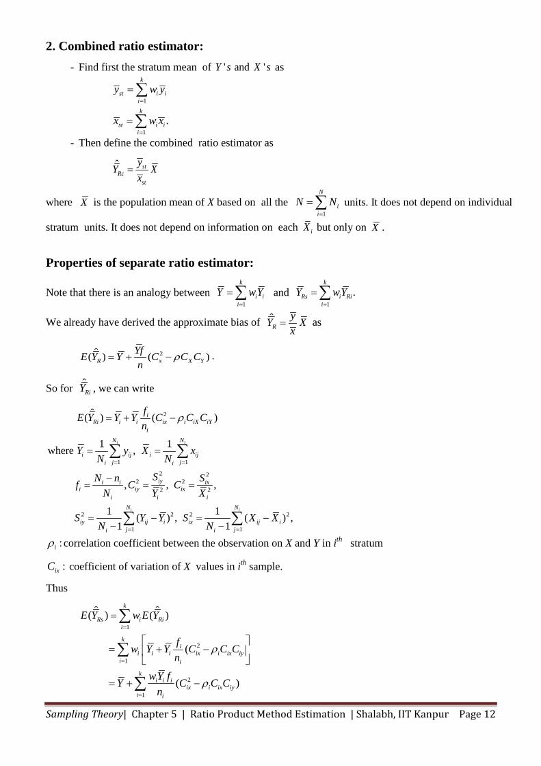
2. Combined ratio estimator: - Find first the stratum mean of ' and 'Y s X s as
1
1.
k
st i iik
st i ii
y w y
x w x
=
=
=
=
∑
∑
- Then define the combined ratio estimator as
ˆ stRc
st
yY Xx
=
where X is the population mean of X based on all the 1
N
ii
N N=
=∑ units. It does not depend on individual
stratum units. It does not depend on information on each iX but only on X .
Properties of separate ratio estimator:
Note that there is an analogy between 1
k
i ii
Y wY=
=∑ and 1
.k
Rs i Rii
Y wY=
=∑
We already have derived the approximate bias of ˆR
yY Xx
= as
2ˆ( ) ( )R x X YYfE Y Y C C Cn
ρ= + − .
So for ˆRiY , we can write
2
1 1
2 22 2
2 2
2 2 2 2
1 1
ˆ ( ) ( )
1 1where ,
, , ,
1 1 ( ) , ( ) ,1 1
i i
i i
iRi i i ix i iX iY
iN N
i ij i ijj ji i
iyi i ixi iy ix
i i iN N
iy ij i ix ij ij ji i
fE Y Y Y C C Cn
Y y X xN N
SN n Sf C CN Y X
S Y Y S X XN N
ρ
= =
= =
= + −
= =
−= = =
= − = −− −
∑ ∑
∑ ∑
:iρ correlation coefficient between the observation on X and Y in ith stratum
:ixC coefficient of variation of X values in ith sample.
Thus
1
2
1
2
1
ˆ ˆ( ) ( )
(
( )
=
=
=
=
= + −
= + −
∑
∑
∑
k
Rs i Rii
ki
i i i ix i ix iyi i
ki i i
ix i ix iyi i
E Y w E Y
fw Y Y C C Cn
wY fY C C Cn
ρ
ρ
Sampling Theory| Chapter 5 | Ratio Product Method Estimation | Shalabh, IIT Kanpur Page 13
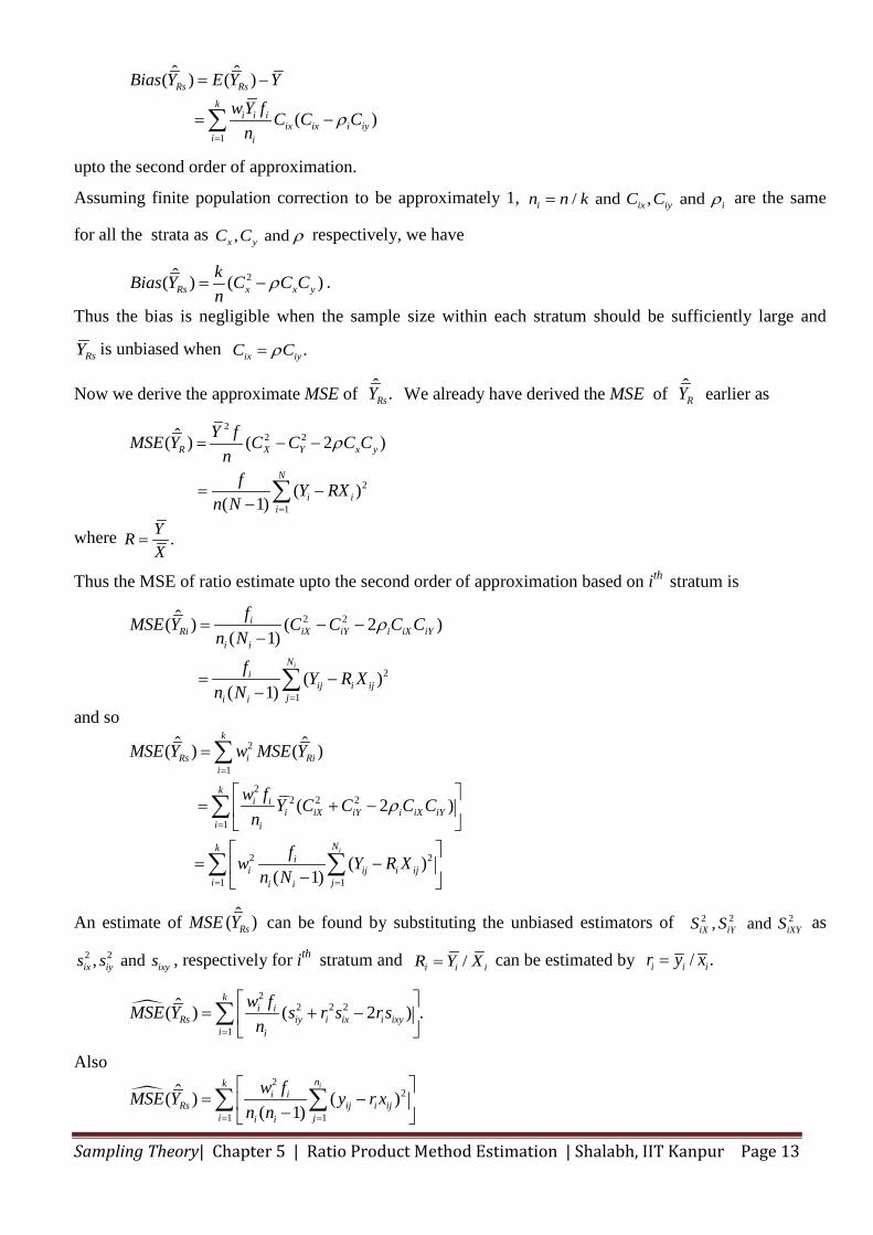
1
ˆ ˆ( ) ( )
( )=
= −
= −∑Rs Rs
ki i i
ix ix i iyi i
Bias Y E Y YwY f C C C
nρ
upto the second order of approximation.
Assuming finite population correction to be approximately 1, / and , andi ix iy in n k C C ρ= are the same
for all the strata as , and x yC C ρ respectively, we have
2ˆ( ) ( )Rs x x ykBias Y C C Cn
ρ= − .
Thus the bias is negligible when the sample size within each stratum should be sufficiently large and
RsY is unbiased when .ix iyC Cρ=
Now we derive the approximate MSE of ˆ .RsY We already have derived the MSE of ˆRY earlier as
22 2
2
1
ˆ( ) ( 2 )
( )( 1)
R X Y x y
N
i ii
Y fMSE Y C C C Cn
f Y RXn N
ρ
=
= − −
= −− ∑
where .YRX
=
Thus the MSE of ratio estimate upto the second order of approximation based on ith stratum is
2 2
2
1
ˆ( ) ( 2 )( 1)
( )( 1)
i
iRi iX iY i iX iY
i iN
iij i ij
ji i
fMSE Y C C C Cn N
f Y R Xn N
ρ
=
= − −−
= −− ∑
and so
2
1
22 2 2
1
2 2
1 1
ˆ ˆ( ) ( )
( 2 )
( )( 1)
i
k
Rs i Rii
ki i
i iX iY i iX iYi i
Nki
i ij i iji ji i
MSE Y w MSE Y
w f Y C C C Cn
fw Y R Xn N
ρ
=
=
= =
=
= + −
= − −
∑
∑
∑ ∑
An estimate of MSE ˆ( )RsY can be found by substituting the unbiased estimators of 2 2 2, andiX iY iXYS S S as
2 2, andix iy ixys s s , respectively for ith stratum and /i i iR Y X= can be estimated by / .i i ir y x=
22 2 2
1
ˆ( ) ( 2 ) .=
= + −
∑
ki i
Rs iy i ix i ixyi i
w fMSE Y s r s r sn
Also
22
1 1
ˆ( ) ( )( 1)= =
= − − ∑ ∑
inki i
Rs ij i iji ji i
w fMSE Y y r xn n
Sampling Theory| Chapter 5 | Ratio Product Method Estimation | Shalabh, IIT Kanpur Page 14
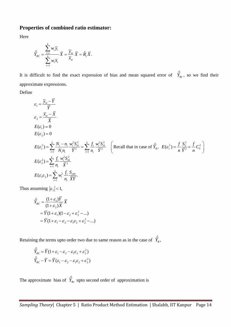
Properties of combined ratio estimator: Here
1
1
ˆ ˆ .
k
i ii st
RC ckst
i ii
w yyY X X R Xxw x
=
=
= = =∑
∑
It is difficult to find the exact expression of bias and mean squared error of ˆRcY , so we find their
approximate expressions.
Define
1
2
1
2
( ) 0( ) 0
st
st
y YY
x XX
EE
ε
ε
εε
−=
−=
==
2 2 2 2 22 2 21 12 2 2
1 1
2 222 2
1
21 2
1
ˆ( ) Recall that in case of , ( )
( )
( ) .
k ki i i iY i i iY Y
R Yi ii i i
ki i iX
i ik
i iXYi
i i
N n w S f w S Sf fE Y E CN n Y n Y n Y n
f w SEn X
f SE wn XY
ε ε
ε
ε ε
= =
=
=
−= = = =
=
=
∑ ∑
∑
∑
Thus assuming 2 1,ε <
1
22
1 2 22
1 2 1 2 2
(1 )ˆ(1 )(1 )(1 ...)(1 ...)
RCYY XX
YY
εε
ε ε ε
ε ε ε ε ε
+=
+
= + − + −
= + − − + −
Retaining the terms upto order two due to same reason as in the case of ˆ ,RY
2
1 2 1 2 2
21 2 1 2 2
ˆ (1 )ˆ ( )
RC
RC
Y Y
Y Y Y
ε ε ε ε ε
ε ε ε ε ε
+ − − +
− = − − +
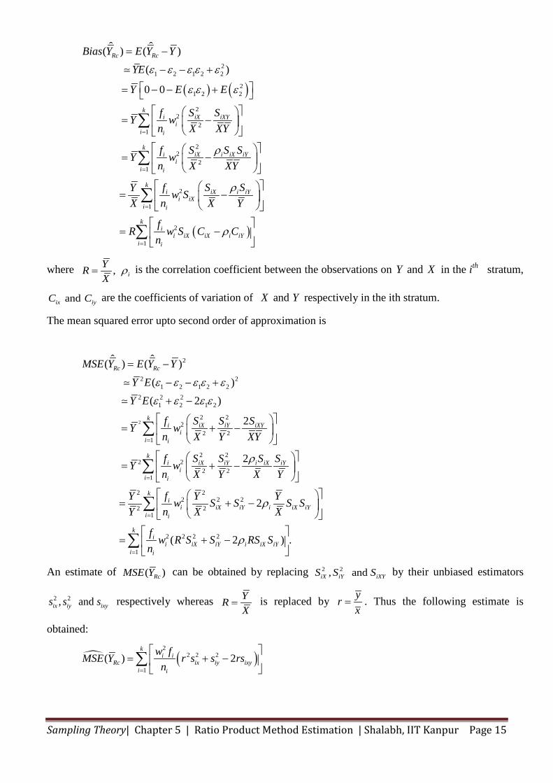
The approximate bias of ˆRcY upto second order of approximation is
Sampling Theory| Chapter 5 | Ratio Product Method Estimation | Shalabh, IIT Kanpur Page 15
( ) ( )2
1 2 1 2 2
21 2 2
22
21
22
21
2
1
2
ˆ ˆ( ) ( )( )
0 0
Rc Rc
ki iX iXY
ii i
ki iX i iX iY
ii i
ki iX i iY
i iXi i
ii iX iX i
i
Bias Y E Y YYE
Y E E
f S SY wn X XY
f S S SY wn X XY
f S SY w SX n X Y
fR w S Cn
ε ε ε ε ε
ε ε ε
ρ
ρ
ρ
=
=
=
= −
− − +
= − − +
= −
= −
= −
= −
∑
∑
∑
( )1
k
iYi
C=
∑
where , iYRX
ρ= is the correlation coefficient between the observations on andY X in the ith stratum,
andix iyC C are the coefficients of variation of andX Y respectively in the ith stratum.
The mean squared error upto second order of approximation is
2
2
2 21 2 1 2 2
2 2 21 2 1 2
2 22
2 21
2 22 2
2 21
2 22 2 2
2 2
ˆ ˆ( ) ( )( )( 2 )
2
2
2
Rc Rc
ki iX iY iXY
ii i
ki iX iY i iX iY
ii i
ii iX iY i iX iY
i
MSE Y E Y YY EY E
f S S SY wn X Y XY
f S S S SY wn X Y X Y
fY Y Yw S S S SY n X X
ε ε ε ε ε
ε ε ε ε
ρ
ρ
=
=
= −
− − +
+ −
= + −
= + −
= + −
∑
∑
1
2 2 2 2
1( 2 ) .
k
i
ki
i iX iY i iX iYi i
f w R S S RS Sn
ρ
=
=
= + −
∑
∑
An estimate of ( )RcMSE Y can be obtained by replacing 2 2, and iX iY iXYS S S by their unbiased estimators
2 2, and ix iy ixys s s respectively whereas YRX
= is replaced by yrx
= . Thus the following estimate is
obtained:
( )2
2 2 2
1( ) 2
ki i
Rc ix iy ixyi i
w fMSE Y r s s rsn=
= + −
∑
Sampling Theory| Chapter 5 | Ratio Product Method Estimation | Shalabh, IIT Kanpur Page 16
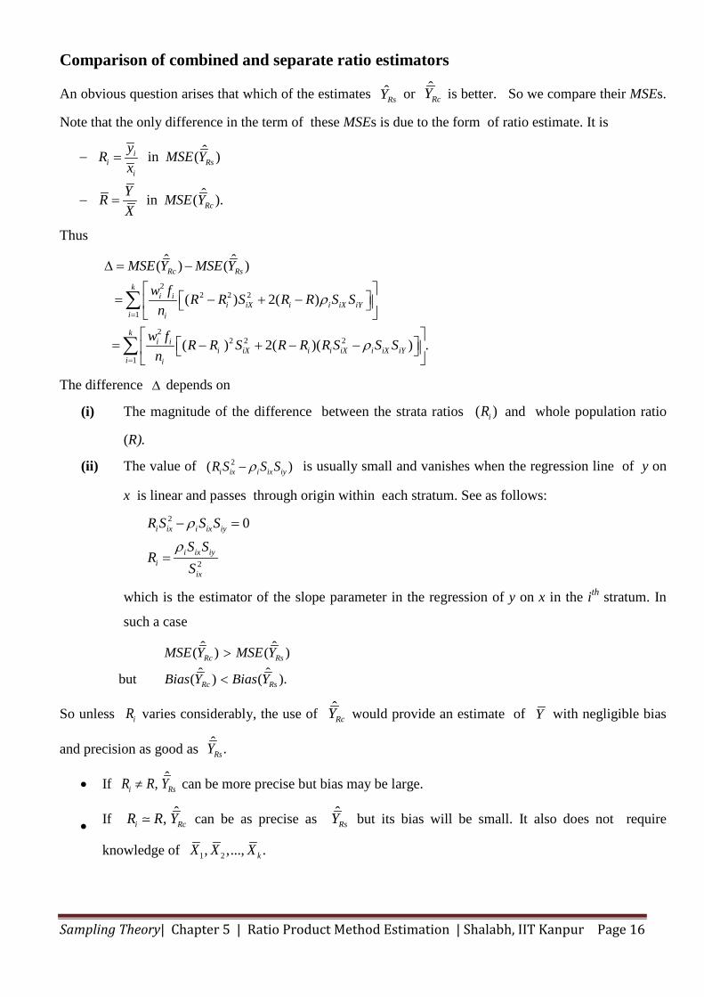
Comparison of combined and separate ratio estimators
An obvious question arises that which of the estimates RsY or ˆRcY is better. So we compare their MSEs.
Note that the only difference in the term of these MSEs is due to the form of ratio estimate. It is
ˆ in ( )
ˆ in ( ).
ii Rs
i
Rc
yR MSE YxYR MSE YX
− =
− =
Thus
22 2 2
1
22 2 2
1
ˆ ˆ( ) ( )
( ) 2( )
( ) 2( )( ) .
Rc Rs
ki i
i iX i i iX iYi i
ki i
i iX i i iX i iX iYi i
MSE Y MSE Y
w f R R S R R S Sn
w f R R S R R R S S Sn
ρ
ρ
=
=
∆ = −
= − + −
= − + − −
∑
∑
The difference ∆ depends on
(i) The magnitude of the difference between the strata ratios ( )iR and whole population ratio
(R).
(ii) The value of 2( )i ix i ix iyR S S Sρ− is usually small and vanishes when the regression line of y on
x is linear and passes through origin within each stratum. See as follows:
2
2
0i ix i ix iy
i ix iyi
ix
R S S SS S
RS
ρ
ρ
− =
=
which is the estimator of the slope parameter in the regression of y on x in the ith stratum. In
such a case
ˆ ˆ ( ) ( )ˆ ˆbut ( ) ( ).
Rc Rs
Rc Rs
MSE Y MSE Y
Bias Y Bias Y
>
<
So unless iR varies considerably, the use of ˆRcY would provide an estimate of Y with negligible bias
and precision as good as ˆ .RsY
• If ˆ,i RsR R Y≠ can be more precise but bias may be large.
• If ˆ,i RcR R Y can be as precise as ˆRsY but its bias will be small. It also does not require
knowledge of 1 2, ,..., .kX X X
Sampling Theory| Chapter 5 | Ratio Product Method Estimation | Shalabh, IIT Kanpur Page 17
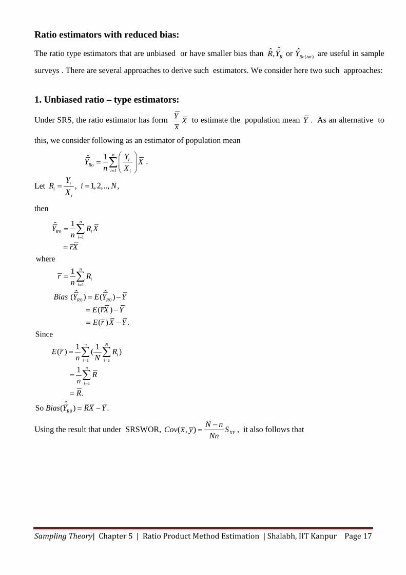
Ratio estimators with reduced bias:
The ratio type estimators that are unbiased or have smaller bias than ( )ˆˆ ˆ, orR Rc totR Y Y are useful in sample
surveys . There are several approaches to derive such estimators. We consider here two such approaches:
1. Unbiased ratio – type estimators:
Under SRS, the ratio estimator has form Y Xx
to estimate the population mean Y . As an alternative to
this, we consider following as an estimator of population mean
1
1ˆ ni
Roi i
YY Xn X=
=
∑ .
Let , 1, 2,.., ,ii
i
YR i NX
= =
then
01
1
0 0
1 1
1
1ˆ
where
1
ˆ ˆ ( ) ( ) ( ) ( ) .
Since1 1 ( ) ( )
1
.ˆSo (
=
=
= =
=
=
=
=
= −
= −
= −
=
=
=
∑
∑
∑ ∑
∑
n
R ii
n
ii
R R
n N
ii i
n
i
Y R XnrX
r Rn
Bias Y E Y YE rX YE r X Y
E r Rn N
RnR
Bias Y 0 ) .= −R RX Y
Using the result that under SRSWOR, ( , ) XYN nCov x y SNn−
= , it also follows that
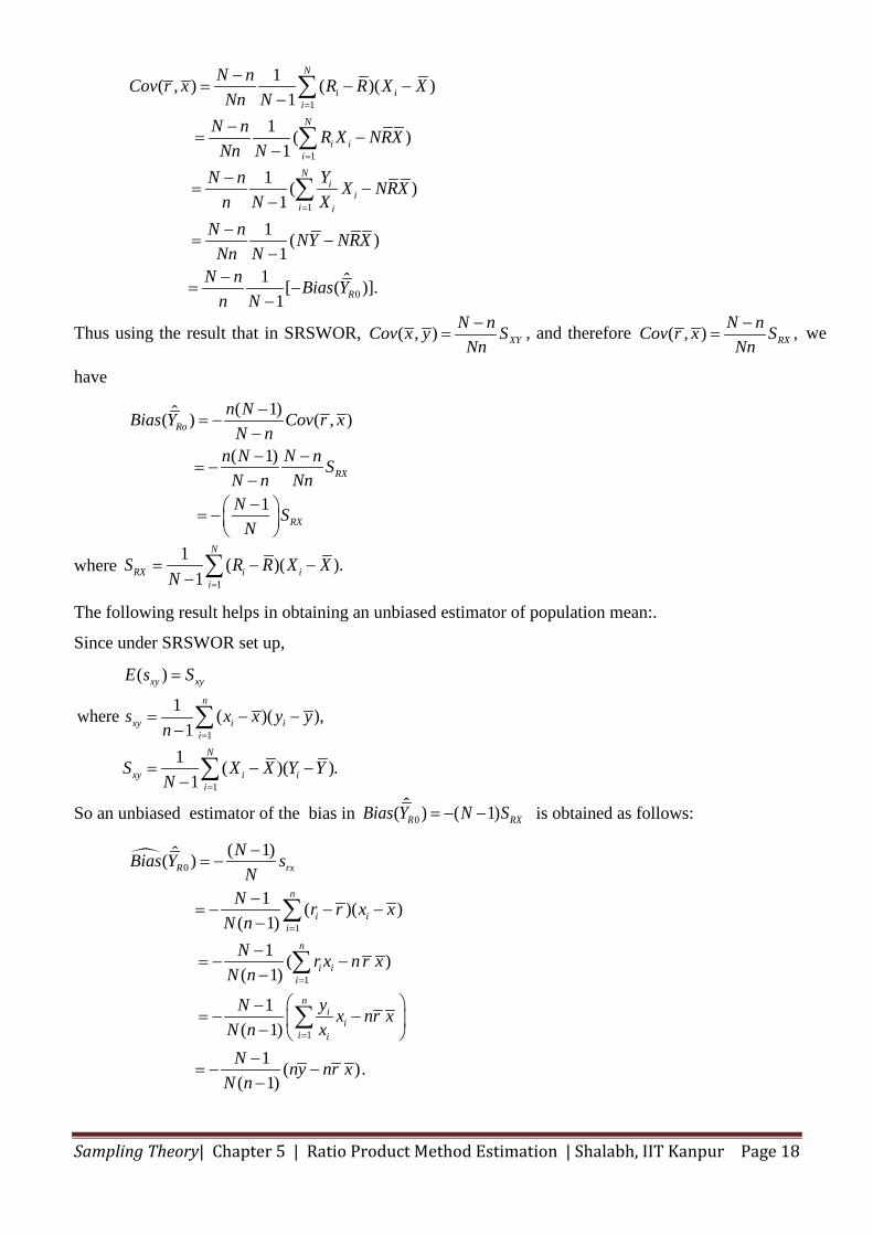
Sampling Theory| Chapter 5 | Ratio Product Method Estimation | Shalabh, IIT Kanpur Page 18
1
1
1
0
1( , ) ( )( )1
1 ( )1
1 ( )1
1 ( )1
1 ˆ[ ( )].1
N
i iiN
i iiN
ii
i i
R
N nCov r x R R X XNn N
N n R X NRXNn N
YN n X NRXn N X
N n NY NRXNn N
N n Bias Yn N
=
=
=
−= − −
−−
= −−
−= −
−−
= −−
−= −
−
∑
∑
∑
Thus using the result that in SRSWOR, ( , ) XYN nCov x y SNn−
= , and therefore ( , ) ,RXN nCov r x SNn−
= we
have
( 1)ˆ( ) ( , )
( 1)
1
Ro
RX
RX
n NBias Y Cov r xN n
n N N n SN n NnN S
N
−= −
−− −
= −−− = −
where 1
1 ( )( ).1
N
RX i ii
S R R X XN =
= − −− ∑
The following result helps in obtaining an unbiased estimator of population mean:.
Since under SRSWOR set up,
1
1
( )
1where ( )( ),1
1 ( )( ).1
xy xy
n
xy i ii
N
xy i ii
E s S
s x x y yn
S X X Y YN
=
=
=
= − −−
= − −−
∑
∑
So an unbiased estimator of the bias in 0ˆ( ) ( 1)R RXBias Y N S= − − is obtained as follows:
0
1
1
1
( 1)ˆ( )
1 ( )( )( 1)
1 ( )( 1)
1( 1)
1 ( ).( 1)
=
=
=
−= −
−= − − −
−
−= − −
−
−= − − −
−= − −
−
∑
∑
∑
R rx
n
i ii
n
i ii
ni
ii i
NBias Y sN
N r r x xN n
N r x n r xN n
yN x nr xN n xN ny nr x
N n
Sampling Theory| Chapter 5 | Ratio Product Method Estimation | Shalabh, IIT Kanpur Page 19
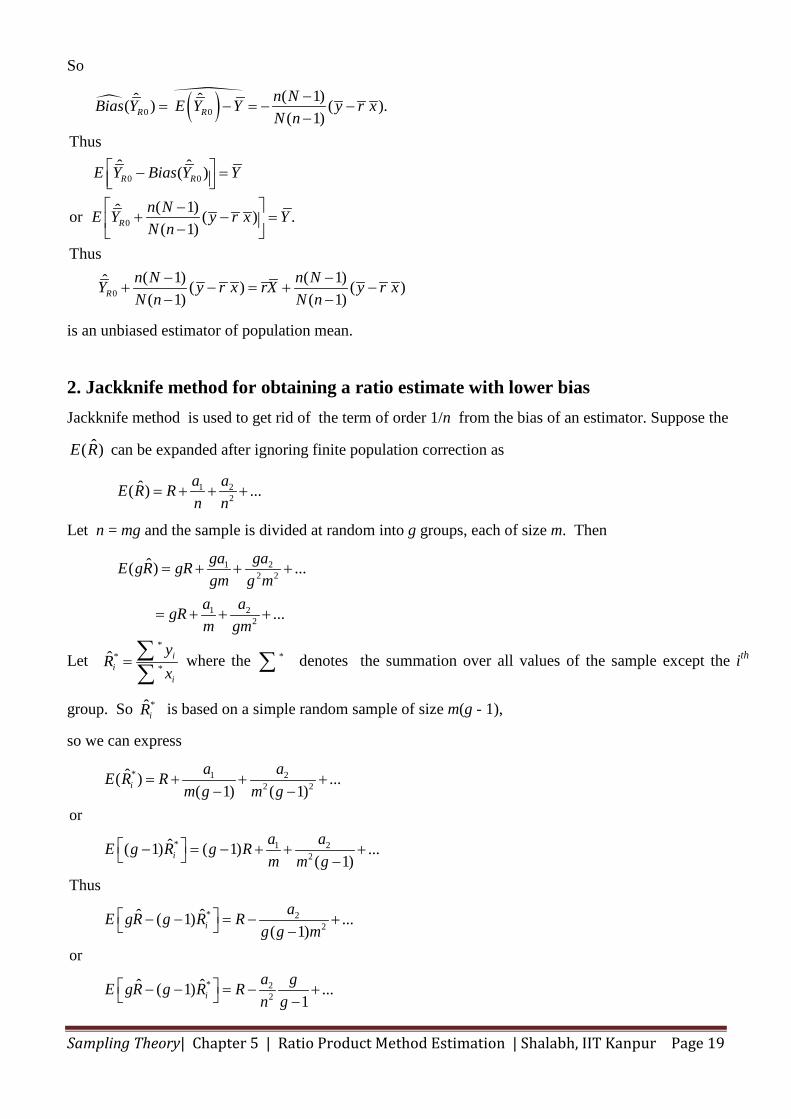
So
( )0 0
0 0
0
0
( 1)ˆ ˆ ( ) ( ).( 1)
Thusˆ ˆ ( )
( 1)ˆor ( ) .( 1)
Thus( 1) ( 1)ˆ ( ) ( )( 1) ( 1)
−= − = − −
−
− = −
+ − = −
− −+ − = + −
− −
R R
R R
R
R
n NBias Y E Y Y y r xN n
E Y Bias Y Y
n NE Y y r x YN n
n N n NY y r x rX y r xN n N n
is an unbiased estimator of population mean.
2. Jackknife method for obtaining a ratio estimate with lower bias Jackknife method is used to get rid of the term of order 1/n from the bias of an estimator. Suppose the
ˆ( )E R can be expanded after ignoring finite population correction as
1 22
ˆ( ) ...a aE R Rn n
= + + +
Let n = mg and the sample is divided at random into g groups, each of size m. Then
1 22 2
1 22
ˆ( ) ...
...
ga gaE gR gRgm g m
a agRm gm
= + + +
= + + +
Let *
**
ˆ ii
i
yR
x= ∑∑
where the *∑ denotes the summation over all values of the sample except the ith
group. So *ˆiR is based on a simple random sample of size m(g - 1),
so we can express
* 1 22 2
* 1 22
* 22
* 22
ˆ ( ) ...( 1) ( 1)
or
ˆ ( 1) ( 1) ...( 1)
Thus
ˆ ˆ ( 1) ...( 1)
or
ˆ ˆ ( 1) ...1
= + + +− −
− = − + + + −
− − = − + −
− − = − + −
i
i
i
i
a aE R Rm g m g
a aE g R g Rm m g
aE gR g R Rg g m
a gE gR g R Rn g
Sampling Theory| Chapter 5 | Ratio Product Method Estimation | Shalabh, IIT Kanpur Page 20
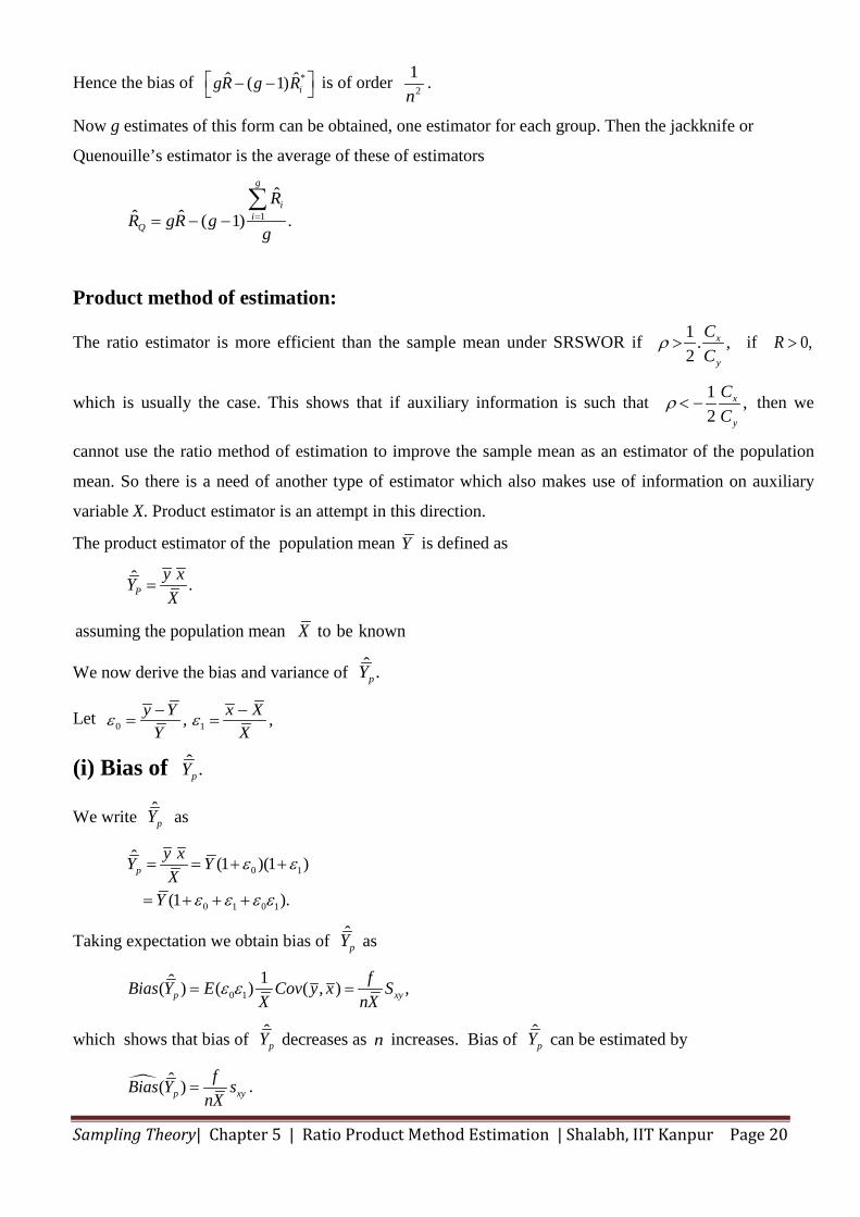
Hence the bias of *ˆ ˆ( 1) igR g R − − is of order 2
1n
.
Now g estimates of this form can be obtained, one estimator for each group. Then the jackknife or
Quenouille’s estimator is the average of these of estimators
1
ˆˆ ˆ ( 1) .
g
ii
Q
RR gR g
g== − −∑
Product method of estimation:
The ratio estimator is more efficient than the sample mean under SRSWOR if 1 . ,2
x
y
CC
ρ > if 0,R >
which is usually the case. This shows that if auxiliary information is such that 1 ,2
x
y
CC
ρ < − then we
cannot use the ratio method of estimation to improve the sample mean as an estimator of the population
mean. So there is a need of another type of estimator which also makes use of information on auxiliary
variable X. Product estimator is an attempt in this direction.
The product estimator of the population mean Y is defined as
ˆ .Py xYX
=
assuming the population mean to be known X
We now derive the bias and variance of ˆ .pY
Let 0 1, ,y Y x XY X
ε ε− −= =
(i) Bias of ˆ .pY
We write ˆpY as
0 1
0 1 0 1
ˆ (1 )(1 )
(1 ).
py xY YX
Y
ε ε
ε ε ε ε
= = + +
= + + +
Taking expectation we obtain bias of ˆpY as
0 11ˆ( ) ( ) ( , ) ,p xy
fBias Y E Cov y x SX nX
ε ε= =
which shows that bias of ˆpY decreases as n increases. Bias of ˆ
pY can be estimated by
ˆ( )p xyfBias Y s
nX= .
Sampling Theory| Chapter 5 | Ratio Product Method Estimation | Shalabh, IIT Kanpur Page 21
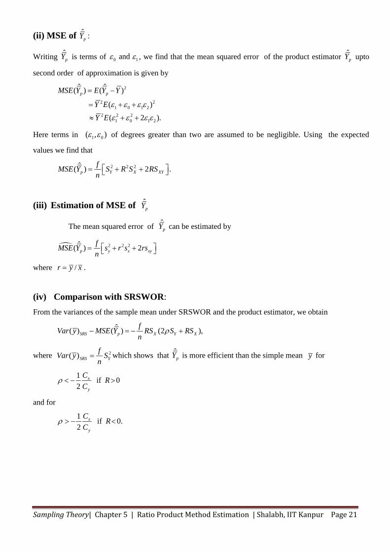
(ii) MSE of ˆ :pY
Writing ˆpY is terms of 0 1andε ε , we find that the mean squared error of the product estimator ˆ
pY upto
second order of approximation is given by
2
2 21 0 1 2
2 2 21 0 1 2
ˆ ˆ( ) ( )
( ) ( 2 ).
p pMSE Y E Y Y
Y EY E
ε ε ε ε
ε ε ε ε
= −
= + +
≈ + +
Here terms in 1 0( , )ε ε of degrees greater than two are assumed to be negligible. Using the expected
values we find that
2 2 2ˆ( ) 2 .p Y X XYfMSE Y S R S RSn = + +
(iii) Estimation of MSE of ˆpY
The mean squared error of ˆpY can be estimated by
2 2 2ˆ( ) 2p y x xyfMSE Y s r s rsn = + +
where /r y x= .
(iv) Comparison with SRSWOR: From the variances of the sample mean under SRSWOR and the product estimator, we obtain
ˆ( ) ( ) (2 ),SRS p X Y XfVar y MSE Y RS S RSn
ρ− = − +
where 2( )SRS YfVar y Sn
= which shows that ˆpY is more efficient than the simple mean y for
1 if 02
x
y
C RC
ρ < − >
and for
1 if 0.2
x
y
C RC
ρ > − <
Sampling Theory| Chapter 5 | Ratio Product Method Estimation | Shalabh, IIT Kanpur Page 22
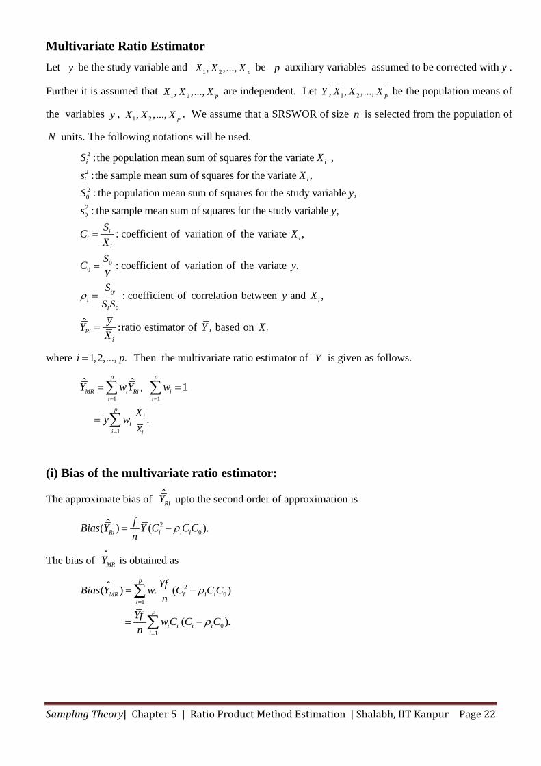
Multivariate Ratio Estimator Let y be the study variable and 1 2, ,..., pX X X be p auxiliary variables assumed to be corrected with y .
Further it is assumed that 1 2, ,..., pX X X are independent. Let 1 2, , ,..., pY X X X be the population means of
the variables y , 1 2, ,..., pX X X . We assume that a SRSWOR of size n is selected from the population of
N units. The following notations will be used.
2
2
2020
: the population mean sum of squares for the variate ,: the sample mean sum of squares for the variate ,: the population mean sum of squares for the study variable ,: the sample mean s
i i
i i
S Xs XS ys
00
0
um of squares for the study variable ,
: coefficient of variation of the variate ,
: coefficient of variation of the variate ,
: coefficient of correlation between and ,
ˆ :ratio estimator o
ii i
i
iyi i
i
Rii
ySC XXSC yYS
y XS S
yYX
ρ
=
=
=
= f , based on iY X
where 1,2,..., .i p= Then the multivariate ratio estimator of Y is given as follows.
1 1
1
ˆ ˆ , 1
.
p p
MR i Ri ii i
pi
ii i
Y wY w
Xy wx
= =
=
= =
=
∑ ∑
∑
(i) Bias of the multivariate ratio estimator:
The approximate bias of ˆRiY upto the second order of approximation is
20
ˆ( ) ( ).Ri i i ifBias Y Y C C Cn
ρ= −
The bias of ˆMRY is obtained as
20
1
01
ˆ( ) ( )
( ).
p
MR i i i ii
p
i i i ii
YfBias Y w C C Cn
Yf w C C Cn
ρ
ρ
=
=
= −
= −
∑
∑
Sampling Theory| Chapter 5 | Ratio Product Method Estimation | Shalabh, IIT Kanpur Page 23
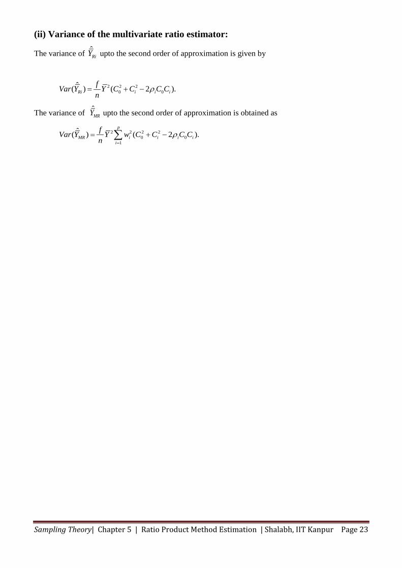
(ii) Variance of the multivariate ratio estimator:
The variance of ˆRiY upto the second order of approximation is given by
2 2 20 0
ˆ( ) ( 2 ).Ri i i ifVar Y Y C C C Cn
ρ= + −
The variance of ˆMRY upto the second order of approximation is obtained as
2 2 2 20 0
1
ˆ( ) ( 2 ).p
MR i i i ii
fVar Y Y w C C C Cn
ρ=
= + −∑