Chapter 5 (cont’d) Costs (Long-Run). Sony Morita: Came to U.S. in 1955 hoping to sell his new...

Chapter 5 (cont’d)

Costs(Long-Run)

Sony• Morita: Came to U.S. in 1955 hoping to sell his

new radio. His story is illustrated in this diagram.

5 10 50 100

Cos

t p

er u

nit

Copyright © Houghton Mifflin Company.All rights reserved. 5b–3

Sony

• Notice that Morita’s curve is U-shaped

• Why?


Production

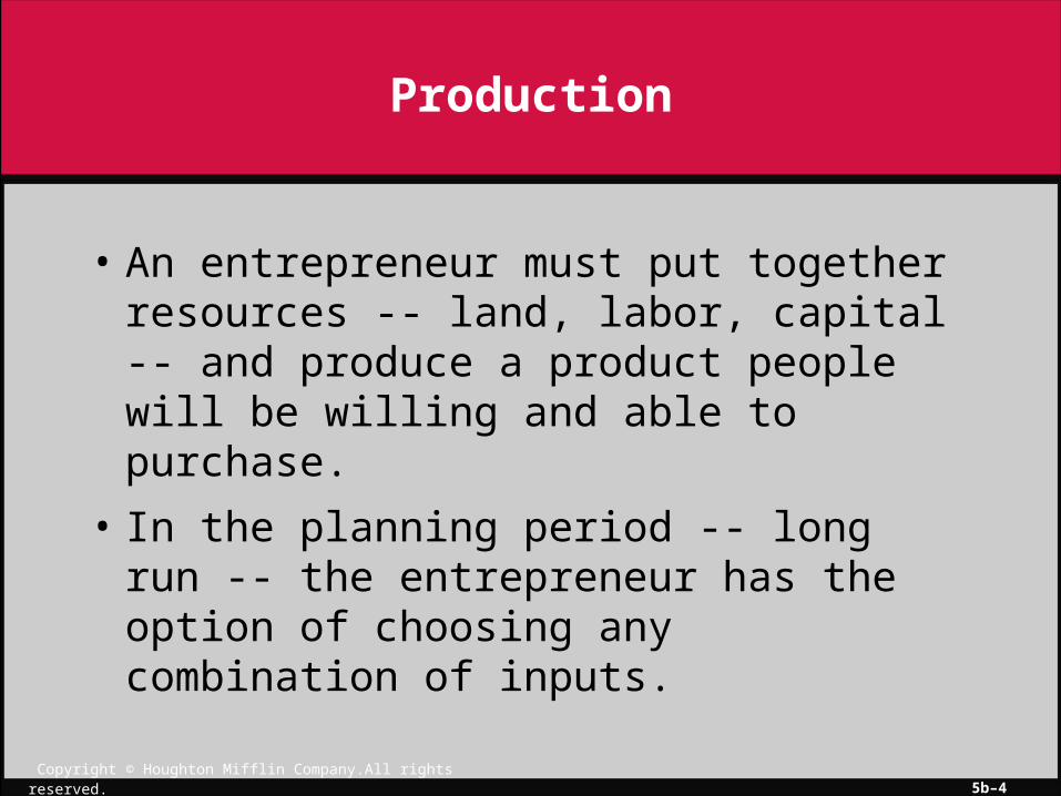
• An entrepreneur must put together resources -- land, labor, capital -- and produce a product people will be willing and able to purchase.

• In the planning period -- long run -- the entrepreneur has the option of choosing any combination of inputs.


Combining Resources

• There are many combinations of resources that could be used.

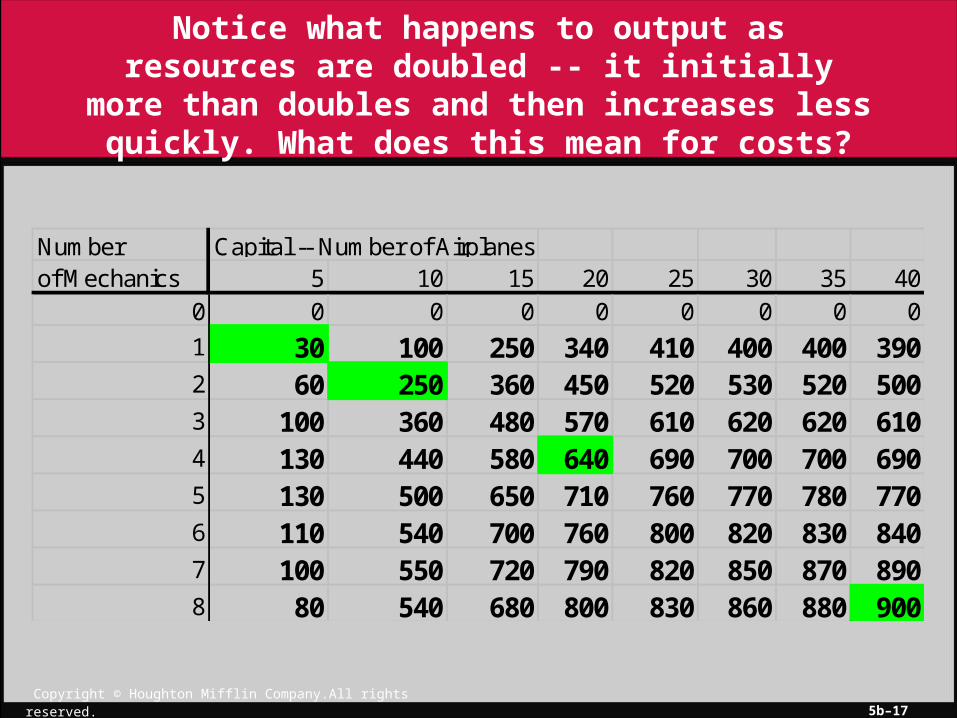
• Consider the following table showing different quantities of mechanics and different quantities of airplanes that the hypothetical airlines PWA might use:


Number Capital -- Number of Airplanesof Mechanics 5 10 15 20 25 30 35 40

0 0 0 0 0 0 0 0 0

1 30 100 250 340 410 400 400 3902 60 250 360 450 520 530 520 5003 100 360 480 570 610 620 620 6104 130 440 580 640 690 700 700 6905 130 500 650 710 760 770 780 7706 110 540 700 760 800 820 830 8407 100 550 720 790 820 850 870 8908 80 540 680 800 830 860 880 900

Alternative Quantities of Output that Can Be Produced by Different Combinations of Resources


Long Run

• What is the difference between the short run and the long run?

• The long run is a period of time just long enough that all resources (inputs) are variable.

• So, in terms of the manufacturing table, we have . . .



0 0 0 0 0 0 0 0 0

1 30 100 250 340 410 400 400 3902 60 250 360 450 520 530 520 5003 100 360 480 570 610 620 620 6104 130 440 580 640 690 700 700 6905 130 500 650 710 760 770 780 7706 110 540 700 760 800 820 830 8407 100 550 720 790 820 850 870 8908 80 540 680 800 830 860 880 900

Alternative Quantities of Output that Can Be Produced by Different

Combinations of ALL Resources


Long Run

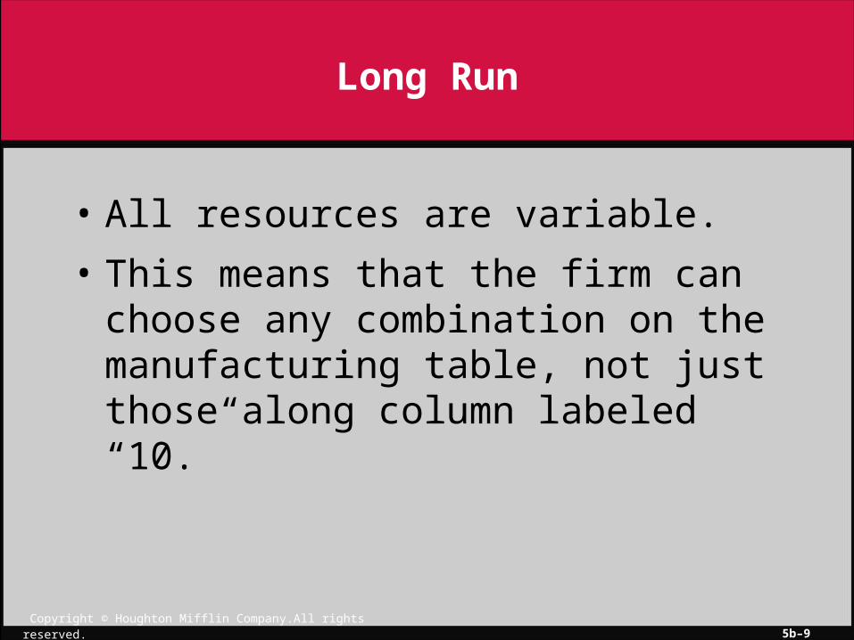
• All resources are variable.

• This means that the firm can choose any combination on the manufacturing table, not just those along column labeled “10.”


Production to Costs

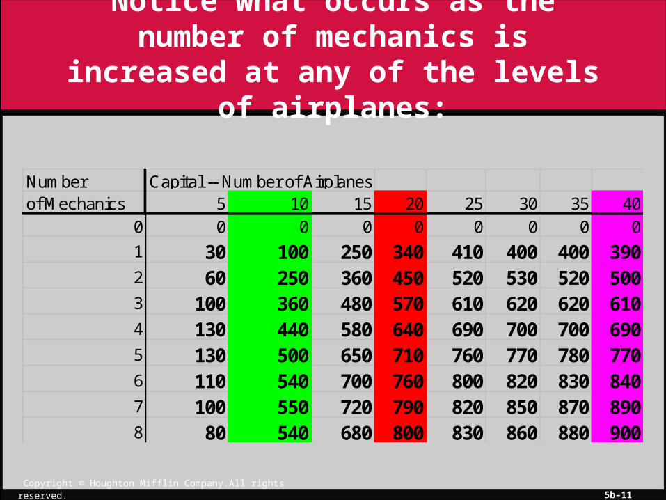
• If either of the resources is fixed, then we get diminishing marginal returns as we increase the other resource.

• For instance, we could fix the number of airplanes at any level, say 10, 20, or 40.

• And vary the number of mechanics.



0 0 0 0 0 0 0 0 0

1 30 100 250 340 410 400 400 3902 60 250 360 450 520 530 520 5003 100 360 480 570 610 620 620 6104 130 440 580 640 690 700 700 6905 130 500 650 710 760 770 780 7706 110 540 700 760 800 820 830 8407 100 550 720 790 820 850 870 8908 80 540 680 800 830 860 880 900

Notice what occurs as the number of mechanics is increased at any of the

levels of airplanes:


Production to Costs

• Or we could fix the number of mechanics and vary the number of airplanes.



0 0 0 0 0 0 0 0 0

1 30 100 250 340 410 400 400 3902 60 250 360 450 520 530 520 5003 100 360 480 570 610 620 620 6104 130 440 580 640 690 700 700 6905 130 500 650 710 760 770 780 7706 110 540 700 760 800 820 830 8407 100 550 720 790 820 850 870 8908 80 540 680 800 830 860 880 900

Notice what occurs to output as the number of airplanes is increased at

any of the levels of mechanics:


Production to Costs

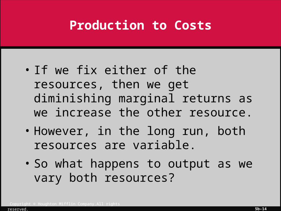
• If we fix either of the resources, then we get diminishing marginal returns as we increase the other resource.

• However, in the long run, both resources are variable.

• So what happens to output as we vary both resources?



0 0 0 0 0 0 0 0 0

1 30 100 250 340 410 400 400 3902 60 250 360 450 520 530 520 5003 100 360 480 570 610 620 620 6104 130 440 580 640 690 700 700 6905 130 500 650 710 760 770 780 7706 110 540 700 760 800 820 830 8407 100 550 720 790 820 850 870 8908 80 540 680 800 830 860 880 900

The Long Run or Planning Period: As we double both resources, what

happens to output?


Scale : Size of Firm

• As the scale or size of the firm is increased, that is, as all resources are increased, what happens to output --- to per-unit costs?

• Since at each fixed level of resources, there are diminishing marginal returns as we vary one of the resources, then there are

• U-shaped cost curves for each scale.



0 0 0 0 0 0 0 0 0

1 30 100 250 340 410 400 400 3902 60 250 360 450 520 530 520 5003 100 360 480 570 610 620 620 6104 130 440 580 640 690 700 700 6905 130 500 650 710 760 770 780 7706 110 540 700 760 800 820 830 8407 100 550 720 790 820 850 870 8908 80 540 680 800 830 860 880 900

Notice what happens to output as resources are doubled -- it initially more than doubles and then increases less quickly. What does this mean for

costs?

Co

sts


Economies of Scale

• As output rises and the scale of the firm increases, costs per unit of output:

• Decrease---called economies of scale.

• Increase---called diseconomies of scale.

• Remain constant---called constant returns to scale.

This is referred to as economies of scaleor size.

Co

sts

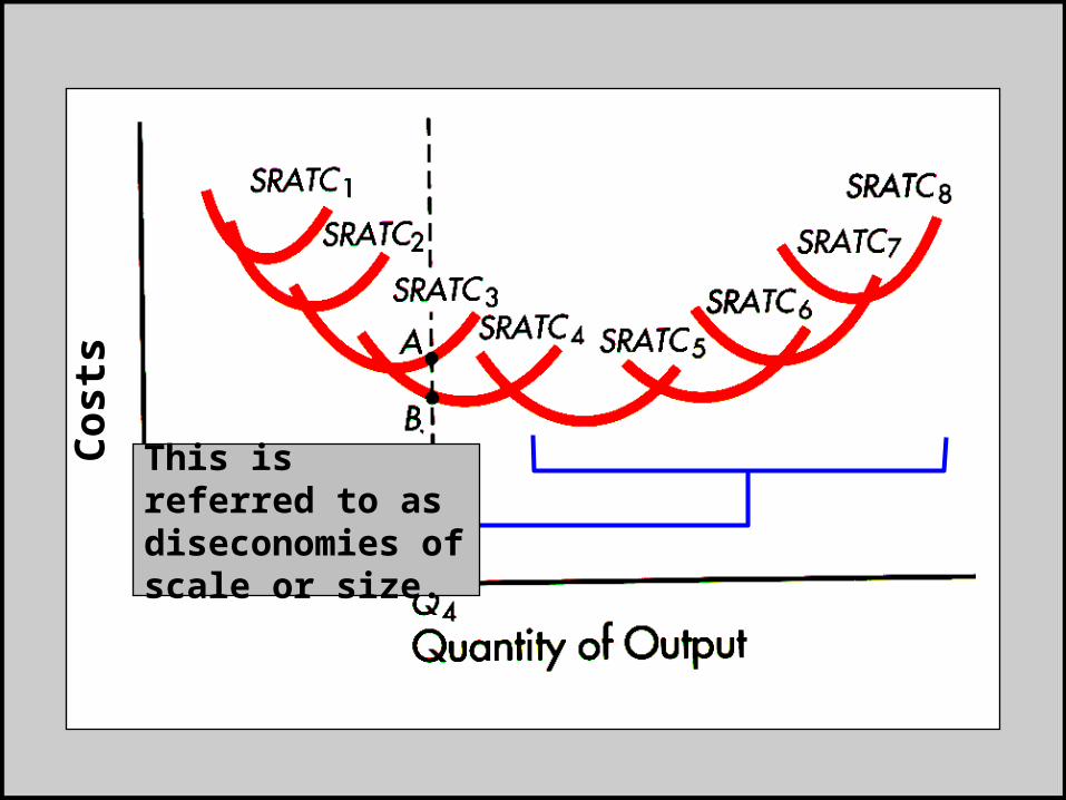
This is referred to as diseconomies of scale or size.

Co

sts


Economies of Scale

• Not all firms or industries have a U-shaped long run cost curve.

• Economies or diseconomies do not come about because of a law like the law of diminishing marginal returns.

• Thus, some industries may have only economies, others only diseconomies, and others constant returns to scale.

Cos

ts

Output

LRATC

What if ATC in the long run looks like this?

Cos

ts

Output

LRATC

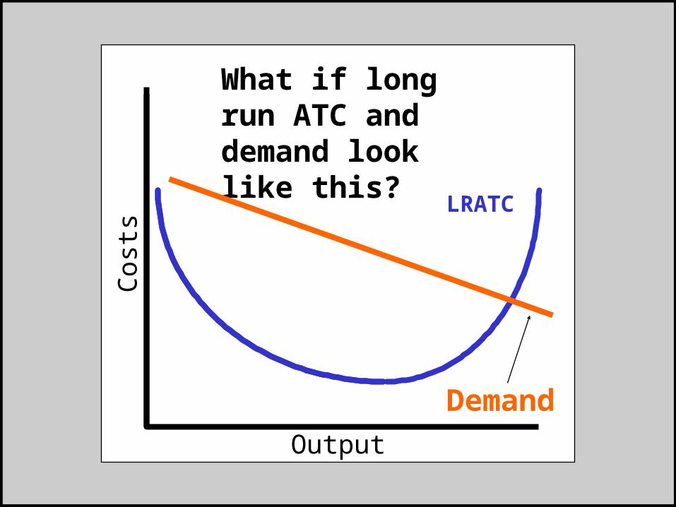
What if long run ATC and demand look like this?

Demand

Cos

ts

Output

LRATC

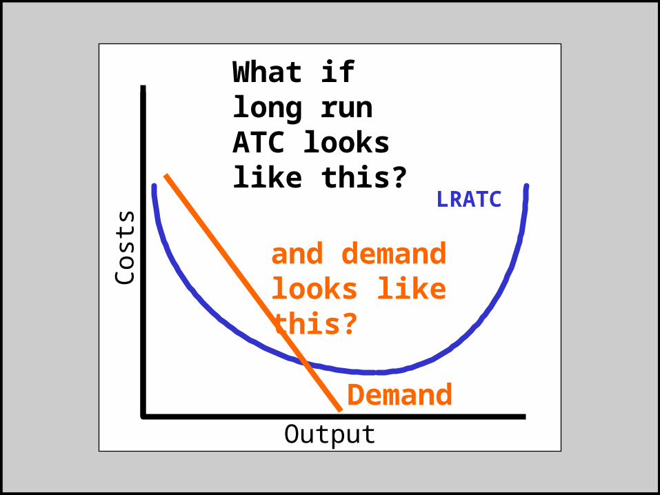
What if long run ATC looks like this?

Cos

ts

Output

LRATC

What if long run ATC looks like this

Demand

and demand like this?

Cos

ts

Output

LRATC


Cos

ts

Output

LRATC

What if long run ATC and demand look like this?

Demand

Cos

ts

Output

LRATC


Demand

and demand looks like this?


Economies of Scope

• Are there per-unit changes in cost resulting from diversifying or expanding the scope of business?

• If cost increases, then there are diseconomies of scope.

• If cost decreases: then there are economies of scope.

Cases: Bayer, BASF, Hoechst

Cases: Advertising agencies

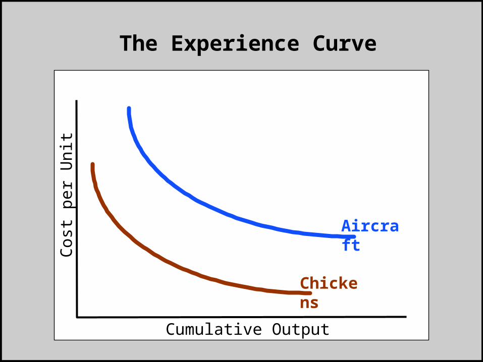
The Experience Curve

Aircraft

Chickens

Cumulative Output

Cos

t per

Uni

t

Aircraft

Chickens

Cumulative Output

Cos

t per

Uni

t The Experience Curve

NOTICE THIS!!!


The Experience Curve

Monsanto vs. Holland Sweetener

• NutraSweet brand -- Monsanto spent 7 years “marching down the learning curve.”


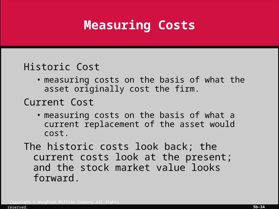
Measuring Costs

Historic Cost• measuring costs on the basis of what the asset

originally cost the firm.

Current Cost• measuring costs on the basis of what a current

replacement of the asset would cost.

The historic costs look back; the current costs look at the present; and the stock market value looks forward.


Measuring Costs

• None of these measures tells us much of use.

• What we really want to know is what the return would be to funds used to purchase assets for this firm if those funds were used in another investment.

• The firm’s performance must be compared to what else the investor’s money could be used for -- the alternatives.

• This is called opportunity cost.


Measuring Costs

• Accountants do not provide information about opportunity costs because it is too subjective and hard to measure.

• There is a move to try to capture opportunity costs: Measuring economic profit has been proposed and adopted by some firms.

• Economic profit =operating profit - (cost of capital)(amount of capital)


Measuring Costs

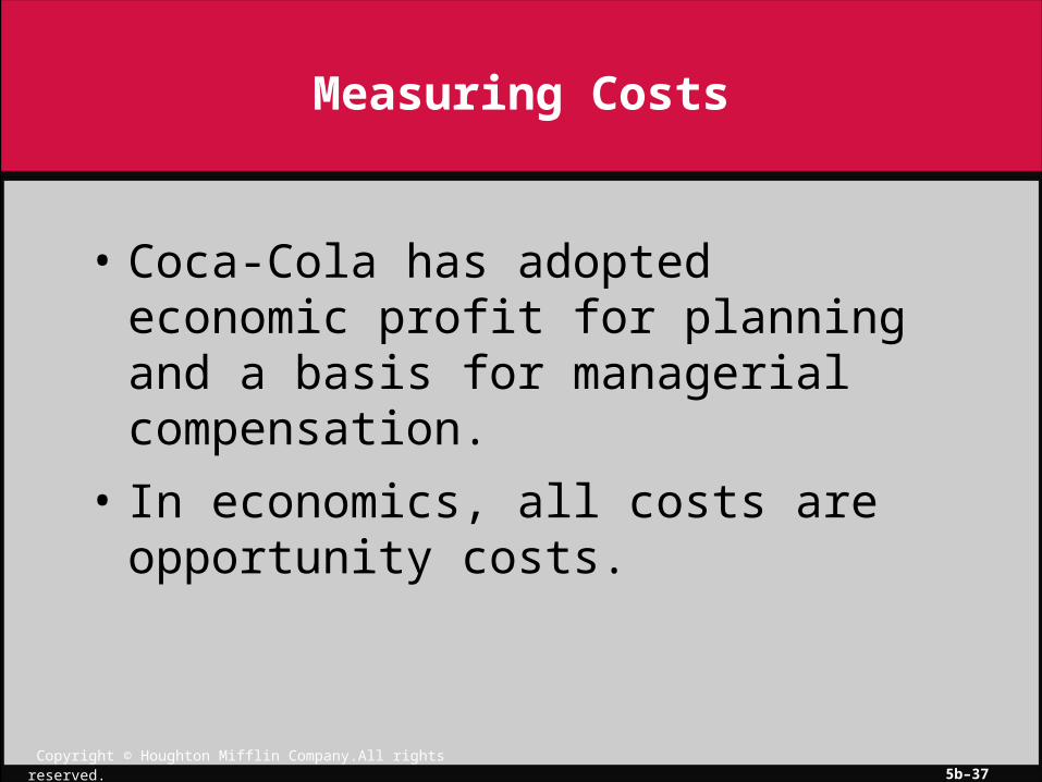
• Coca-Cola has adopted economic profit for planning and a basis for managerial compensation.

• In economics, all costs are opportunity costs.


Measuring Costs

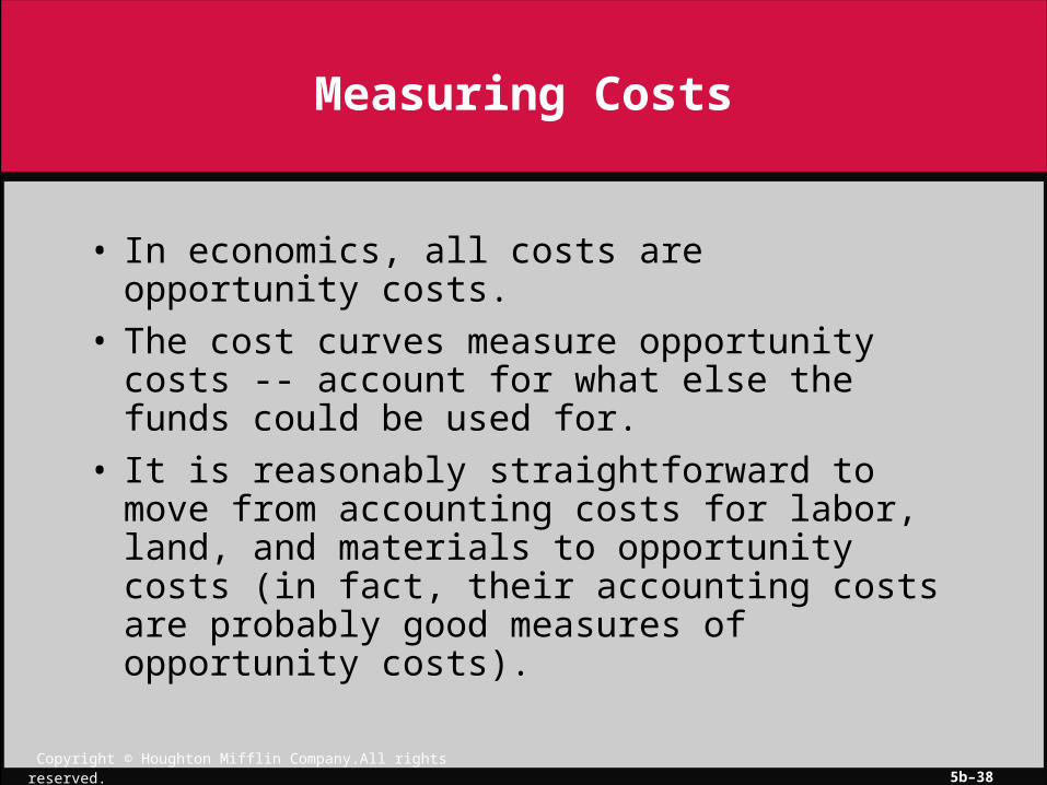
• In economics, all costs are opportunity costs.

• The cost curves measure opportunity costs -- account for what else the funds could be used for.

• It is reasonably straightforward to move from accounting costs for labor, land, and materials to opportunity costs (in fact, their accounting costs are probably good measures of opportunity costs).


Measuring Costs

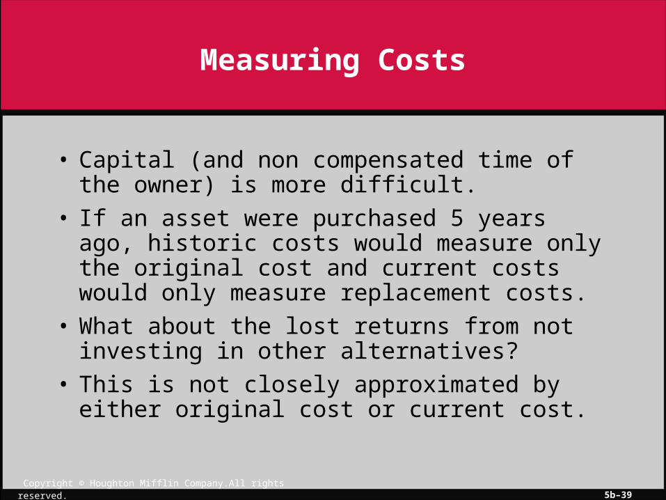
• Capital (and non compensated time of the owner) is more difficult.

• If an asset were purchased 5 years ago, historic costs would measure only the original cost and current costs would only measure replacement costs.

• What about the lost returns from not investing in other alternatives?

• This is not closely approximated by either original cost or current cost.


Measuring Costs

• Thus, you might compare the returns to what a marginal firm would have to pay to acquire the asset.

• A marginal firm is a firm that is neither adding value nor subtracting it.

• It is typically the firm in the industry that is at the bottom of the rung---without going out of business,

• Consider the following situations:

$

output

AVC

ATC

Demand1

What is the situation depicted here? What is the green line?

$

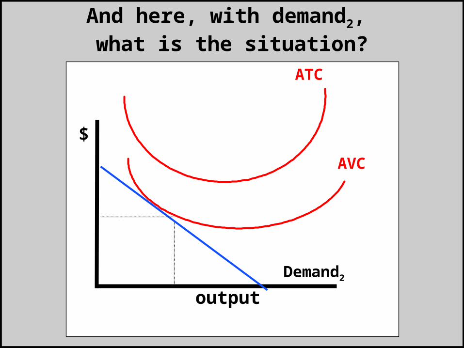
output

AVC

ATC

Demand2

And here, with demand2, what is the situation?

$

output

AVC

ATC

Demand3

Now, at demand3 , what is the situation? What is the green line?


Summary Review of Costs

• Scale -- Long Run• Economies of Scale

• Diseconomies of Scale

• Returns to Scale

• Constant Returns to Scale

• Minimum Efficient Scale

• Returns or Product -- Short Term• Diminishing Marginal Returns

• Diminishing Marginal Product

$

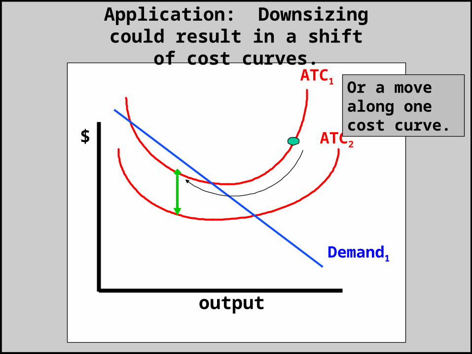
output

ATC2

ATC1

Demand1

Application: Downsizing could result in a shift of cost curves.

Or a move along one cost curve.


Outsourcing and Joint Ventures

• Outsourcing would be illustrated not much differently than the previous case of downsizing.

• The size of the firm would decrease in the case of outsourcing – efficiency should increase.

• In the case of a joint venture, many alternative things might happen: reduced costs, decreased size, increased demand, or increased size and increased efficiency.

Chapter 5 (cont’d) Costs (Long-Run). Sony Morita: Came to U.S. in 1955 hoping to sell his new...

Documents

Transcript of Chapter 5 (cont’d) Costs (Long-Run). Sony Morita: Came to U.S. in 1955 hoping to sell his new...