Chapter 4: Moment Invariants for Image Symmetry Estimation...

CHAPTER 4

Moment Invariants for Image Symmetry Estimation and

Detection

Miroslaw Pawlak

We give a general framework of statistical aspects of the problem of understandingand a description of image symmetries, by utilizing the theory of moment invariants.In particular, we examine the issues of joint symmetry estimation and detection. Thesequestions are formulated as the statistical decision and estimation problems since wecope with images observed in the presence of noise. The estimation/detection proce-dures are based on the minimum L2-distance between the reconstructed image functionand the reconstruction of its hypothesized symmetrical version. Our reconstruction al-gorithms are relying on a class of radial orthogonal moments. The proposed symmetryestimation and detection techniques reveal some statistical optimality properties. Ourtechnical developments are based on the statistical theory of nonparametric testingand semi-parametric inference.

Miroslaw PawlakElectrical and Computer Engineering, University of ManitobaWinnipeg, Canadae-mail: [email protected]

Editor: G.A. Papakostas, Moments and Moment Invariants - Theory and Applications

DOI: 10.15579/gcsr.vol1.ch4, GCSR Vol. 1, c©Science Gate Publishing 201491

92 M. Pawlak

4.1 Introduction

Symmetry plays an important role in signal and image understanding, compression,recognition and human perception [18]. In fact, symmetric patterns are common innature and in man-made objects thus estimation and detection of image symmetriescan be useful for designing e�cient algorithms for object recognition, robotic manip-ulation, image animation, and image compression [11]. Though symmetry can bediscussed from di�erent point of views, in this chapter statistical aspects of spatialsymmetry are examined and reviewed. We are aiming at the fundamental problemsof estimating symmetry parameters like the angle of the axis of mirror symmetry anddetection of symmetry type.For objects represented by a function f that belongs to the space F one can de�ne asymmetry class on F as follows

S = {f ∈ F : f = τθf, θ ∈ Θ}, (4.1)

where τθ is mapping τθ : F → F that represents the transformed version of f . Themapping τθ is parametrized by θ ∈ Θ, where typically Θ is a compact subset of Rp.Hence, the class S is a subset of F de�ning all objects from F that are symmetricwith respect to the class of operations {τθ} parametrized by θ ∈ Θ .In the concrete situation of image analysis an object f is identi�ed with the grey-

level bivariate image function f(x, y). In this case there are two basic symmetry types,i.e., mirror (re�ection) and rotational symmetries. In the former case there is an axisof symmetry that divides the image into two identical re�ected images. Formally, theimage reveals the mirror symmetry if it belongs to the following class

Sm = {f ∈ F : f(x, y) = τmθ f(x, y), θ ∈ Θ}, (4.2)

whereτmθ f(x, y) = f(x cos(2θ) + y sin(2θ), x sin(2θ)− y cos(2θ))

is the re�ection of the image f(x, y) with respect to the axis of symmetry de�ned bythe angle θ ∈ Θ ⊂ [0, π). In rotation symmetry there is a single rotation point suchthat the image rotated about this point by a fraction (degree) of a full cycle alignswith the original image. The corresponding rotation symmetry class Sr is de�ned asin (4.2) with the rotation transformation through the angle θ de�ned as

τ rθ f(x, y) = f(x cos(θ) + y sin(θ),−x sin(θ) + y cos(θ)).

The rotation angle θ takes commonly the form θ = 2π/d, where d is an integer calledthe rotation degree and the corresponding class Sr is referred to as the d-fold rotationsymmetry class.It is also convenient to express the above symmetry constrains in terms of polar co-

ordinates. Hence, let f(ρ, ϕ) be the version of the image function in polar coordinates.Then, the mapping in (4.2) is given by

τmθ f(ρ, ϕ) = f(ρ, 2θ − ϕ) (4.3)

with the corresponding symmetry requirement f(ρ, ϕ) = f(ρ, 2θ − ϕ) for some angleθ. Common mirror symmetry classes are: vertical symmetry (θ = π/2), horizontal

Moment Invariants for Image Symmetry Estimation and Detection 93

symmetry (θ = 0), and diagonal symmetry (θ = π/4). Analogously, the d-fold rotationclass in polar coordinates is de�ned by the mapping

τ rθ f(ρ, ϕ) = f(ρ, ϕ− 2π/d) (4.4)

and the corresponding symmetry requirement f(ρ, ϕ) = f(ρ, ϕ − 2π/d) for somedegree d. There are a few important values of d: d = 2 gives the rotation class by π,d = 4 de�nes the rotation class by π/2. The limit value d =∞ corresponds to radialimages, i.e., when f(ρ, ϕ) = g(ρ) is a function of the radius ρ only for some univariatefunction g.The aforementioned transformations can be combined to de�ne joint symmetries.

For example, one can consider a joint symmetry with respect to the horizontal andvertical transformations. We can easily verify that τmπ/2τ

m0 f = τ rπf and τ rπτ

mπ/2f

= τm0 f . Hence, the symmetry group generated by {τm0 , τmπ/2} is identical to that

generated by {τmπ/2, τrπ}. Thus, one can consider the symmetry class generated jointly

by the vertical re�ection τmπ/2 and the 2-fold rotation τ rπ . Generally, a symmetry group

generated by two re�ections can always be generated by a re�ection and a rotation.In real-world applications we do not have a complete information about the image

function f and one must verify the question whether f reveals some type of symmetryobserving only its discrete and noisy version. In fact, in image processing systems oneneeds to address the following fundamental issues:

1. Detection of the type of symmetry present in the original unobserved image.

2. Estimating the parameters characterizing the given type of symmetry, i.e., theangle of mirror symmetry and the degree of rotational symmetry.

Moreover, we need to estimate the location of symmetry axis and the point of rotation.These problems, however, can be easily resolved by a proper image normalization.Throughout this chapter, we assume that these points are located in the coordinatesystem origin being the image center of inertia.In this chapter, we assume that the only information we have about the original

image function is its noisy and digitized version. Hence, suppose we have discretenoisy image data observed over the region D

Zi,j = f(xi, yj) + εi,j , (xi, yj) ∈ D, 1 ≤ i, j ≤ n, (4.5)

where the noise process {εi,j} is a random sequence with zero mean and �nite varianceσ2ε . The data are observed on a symmetric square grid of edge width ∆, i.e., xi−xi−1 =yi − yi−1 = ∆ and (xi, yj) is the center of the pixel (i, j). Note that ∆ is of order1/n and the image size is n2.We may believe that hidden in the noisy data {Zi,j , 1 ≤ i, j ≤ n} our image exhibits

the one of the aforementioned symmetry type τθ0 for some θ0 ∈ Θ. Thus, we wish todetect the symmetry type τ and estimate the corresponding true symmetry parameterθ0 from {Zi,j , 1 ≤ i, j ≤ n}. The statistical nature of the observed image data andthe lack of any a priori knowledge of the shape of the underlying image f(x, y) call forformal nonparametric statistical methods for joint estimating and testing the existingsymmetry in an image function.

94 M. Pawlak

To appreciate the di�culty of the posed problem we display in Fig.(4.1) the discreteand noisy image that represents the true mirror symmetric image f(x, y) (shown on theleft-hand-side) observed over the rectangular region with the resolution n×n = 30×30.The problem of detection and estimation of the existing symmetry in f(x, y) basedmerely on {Zi,j} is clearly challenging.

(a) (b)

Figure 4.1: (a) The original mirror symmetric image f(x, y). (b) The discrete andnoisy version {Zi,j} of the image in (a).

Some preliminary studies examining statistical aspects of symmetry estimation anddetection have been initiated in [2, 3, 4, 16]. In this chapter, we propose a systematicand rigorous statistical approach for joint estimating and testing of the aforementionedimage symmetries. To do so, we use the orthogonal moments image representationutilizing the theory of radial functions expansions [16, 20]. In particular, we selectthe speci�c radial basis commonly referred to as Zernike functions [1]. The Zernikefunctions de�ne an orthogonal and rotationally invariant basis of radial functions on theunit disk. As such, the Zernike functions and their corresponding Fourier coe�cients(moments) have been extensively used in pattern analysis [10, 17, 16, 20].Our estimation and test statistics are constructed by expressing the symmetry con-

dition in terms of restrictions on radial moments. The estimation procedure is basedon minimizing over θ ∈ Θ the L2 distance between empirical versions of f and τθfde�ning the aforementioned symmetry classes. Hence, f and τθf are estimated usingtruncated radial series with empirically determined Fourier coe�cients. The inherentsymmetry property of radial moments results in a particularly simple procedure forestimating θ.The aforementioned estimation problem is closely connected to the problem of sym-

metry detection based also on the concept of the L2 minimum distance principle.Hence, we wish to verify the following null hypothesis

H0 : f = τθ0f (4.6)

for some θ0 ∈ Θ, against the alternative

Ha : f 6= τθf (4.7)


for all θ ∈ Θ, where τθ is one of the above discussed symmetry classes. For a suchformulated symmetry testing problem we propose detection statistics for which weestablish asymptotic distributions, both under the null hypothesis of symmetry as wellas under �xed alternatives. These results allow us to construct practical tests forthe lack of symmetry and evaluate the corresponding power. Our results model theperformance of our estimates and tests on the grid which becomes increasingly �ne,i.e., when ∆→ 0.The chapter is organized as follows. In Section 4.2 we introduce our basic math-

ematical tools for representing the image symmetries in terms of radial moments.Section 4.3 is dealing with the symmetry estimation problem, whereas Section 4.4examines the issue of symmetry detection.

4.2 Radial Moments and Image Symmetries

The symmetry constrains introduced in the previous section are convenient to expressin some transform domain where we can parametrize the symmetry concept and toform estimates for symmetry detection and recovery. Let us begin with the classicalgeometric moments of the so-called complex form (complex moments) [7, 15]. Hence,let

Cpq(f) =

¨D

zpz∗qf(x, y)dxdy,

be the (p, q)-order complex moment of f , where z = x + jy and z∗ = x − jy is theconjugate of z. In polar coordinates Cpq(f) can be expressed as

Cpq(f) =

ˆ R

0

ˆ 2π

0

ρp+qej(p−q)ϕf(ρ, ϕ)ρdρdϕ,

where R de�nes the range of the image domain D. Let us now express the symmetryconditions in terms of Cpq(f). Owing to the above representation of Cpq(f) in termsof polar coordinates and Eq.(4.3) we can readily obtain that the complex moment ofthe image re�ected by the axis tilted by the angle θ takes the following form

Cpq(τmθ f) = ej(p−q)2θC∗pq(f).

The mirror symmetry condition implies that we must have

ej(p−q)2θC∗pq(f) = Cpq(f). (4.8)

This equation puts some constrains on the admissible set of {Cpq(f)} for whichEq.(4.8) holds. In fact, we can readily derive that if Cpq(f) 6= 0 then Eq.(4.8) isequivalent to

arg(Cpq(f)) = (p− q)θ,where arg(Cpq(f)) is the phase of Cpq(f). In particular, for the horizontal re�ectionthis implies that Cpq(f) must be real, whereas for the vertical re�ection we must havethat arg(Cpq(f)) = (p− q)π/2. Analogously by making use of Eq.(4.4) the complexmoment of the image rotated by the angle θ we obtain

Cpq(τrθ f) = ej(p−q)θCpq(f).

96 M. Pawlak

This yields that for the image exhibiting the d-fold rotation symmetry we have

ej(p−q)2π/dCpq(f) = Cpq(f). (4.9)

This equation holds if we either have the constrain that (p − q)/d is an integer orthat Cpq(f) = 0. All the aforementioned formulas reveal that the classical complexmoments must meet some restrictive constrains on (p, q) in order to capture thesymmetry property of the image. Moreover, complex moments are not orthogonal andas such they exhibit some information redundancy and inability to uniquely recover theimage function from imprecise data as in the noise model de�ned in Eq.(4.5). Thereis also little known about the accuracy of computing Cpq(f) from digital and noisydata.The function space F representing all images can be selected as L2(D) - the space

of square integrable functions de�ned on a compact subset D of R2. This functionclass allows us to represent images in terms of the orthogonal expansions of radialfunctions. It is also important to use the representation that can easily incorporatesymmetry properties of the image. In [1] it is shown that a basis that is invariant inform for any rotation of axes must be of the form

Vpq(x, y) = Rp(ρ)ejqϕ, (4.10)

where the right-hand-side is expressed in polar coordinates (ρ, ϕ). Here, Rp(ρ) is aradial orthogonal polynomial of degree p and q de�nes the angular order. There arevarious ways of selecting Rp(ρ) and important examples are Fourier-Mellin, pseudo-Zernike and Zernike radial bases [7, 17, 16, 20]. Among the possible choices for Rp(ρ)there is only one orthogonal set, the set of Zernike functions, for which Rp(ρ) = Rpq(ρ)is the radial orthogonal polynomial of degree p ≥ |q| such that p−|q| is even [1]. Hence,the Zernike polynomial Rpq(ρ) has no powers of ρ lower than |q|. In this chapter,without loss of generality, we con�ne our derivations and results to the Zernike basis.Analogous discussion can be carried out to other radial orthogonal basis.An image function f ∈ L2(D) can be represented by the N th-term expansion with

respect to the given radial basis {Vpq(x, y)}

fN (x, y) =

N∑p=0

p∑q=−p

λ−1p Apq(f)Vpq(x, y), (4.11)

where λp = ‖Vpq‖2= 2π‖Rpq‖2 is the normalizing constant and ‖ · ‖ denotes theL2 norm. In the case of Zernike polynomials we have ‖Rpq‖2 = 1/2(p + 1) yieldingλp = π/(p+1). Furthermore, the summation in Eq.(4.11) is taken with respect to theadmissible pairs (p, q), i.e., p ≥ |q| and p − |q| is even. Moreover, the image domainD is the unit disk. Then, the radial Zernike moment Apq(f) of the image f is de�nedas follows

Apq(f) =

¨D

f(x, y)V ∗pq(x, y) dx dy.

It is also very useful to express Apq(f) in polar coordinates

Apq(f) =

ˆ 2π

0

ˆ 1

0

f(ρ, ϕ)e−jqϕRpq(ρ) ρ dρdϕ. (4.12)


For future developments we need an expression on the L2 distance between two imagesthat can be expressed in terms of Zernike moments. Recalling Parseval's formula wehave

‖f − g‖2 =

∞∑p=0

λ−1p

p∑q=−p

|Apq(f)−Apq(g)|2. (4.13)

In the following we shall work with an estimated version of the Zernike moments,since the only knowledge about the image function f is given by the data set {Zi,j}generated according to the model in Eq.(4.5). Hence, consider the weights

wpq(xi, yj) =

¨Πij

V ∗pq(x, y) dxdy, (4.14)

where Πij =[xi − ∆

2 , xi + ∆2

]×[yj − ∆

2 , yj + ∆2

]denotes the pixel centered at

(xi, yj). Consequently, the Zernike moment Apq(f) is estimated by

Apq =∑

(xi,yj)∈D

wpq(xi, yj)Zi,j , (4.15)

where the weights are given by Eq.(4.14). A simple approximation for wpq(xi, yj) isgiven by ∆2V ∗pq(xi, yj), see [10, 17, 16] for higher order approximation schemes. The

estimate Apq is a consistent estimate of the true Apq. In fact, the bias E{Apq} =

Apq + O(∆) for a large class of image functions, whereas the variance V ar{Apq}is of order σ2

επp+1∆2. As a result, we have that Apq tends (in probability sense) to

Apq as ∆ → 0. Hence, for high resolution images the invariant property of Apqdiscussed below is approximately satis�ed by Apq. It is also worth mentioning thatalong the boundary of the disk, some pixels are included and some are excluded. Whenreconstructing f from {Apq} this gives rise to an additional error called geometric error.This will be quanti�ed in our considerations by the factor γ < 1.5, see [10, 17, 16] fora discussion of this important problem.As a result, an estimate of the image function f(x, y) from {Apq} is given by

fN (x, y) =

N∑p=0

p∑q=−p

λ−1p ApqVpq(x, y), (4.16)

where N is a smoothing parameter which determines the number of terms in thetruncated Zernike series. It was shown in [10, 17, 16] that the mean integrated

square reconstruction error MISE(fN ) = E˜D|fN (x, y) − f(x, y)|2dxdy satis�es

the propertyMISE(fN∗) = O(∆2/3) (4.17)

provided that the truncation parameter N is selected optimally as N∗ = a∆−2/3 someconstant a. Other choices of N leads to slower decay of the error as ∆ gets smaller,i.e., when the image resolution increases.The fundamental property of radial moments and Zernike moments in particular

is the easiness to embed the basic symmetry transformations into the radial moment

98 M. Pawlak

formula in Eq.(4.12). In fact, recalling the symmetry mappings de�ned in Eq.(4.3)and Eq.(4.4) and the formula in Eq.(4.12) we can obtain the following relationships

Apq(τmθ f) = e−2jqθA∗pq(f) (4.18)

andApq(τ

rθ f) = e−jqθApq(f) (4.19)

for mirror and rotation symmetry mappings, respectively. The symmetry conditionscan be now easily expressed in terms of Apq(f). Hence, the image f exhibits themirror symmetry if

e−2jqθA∗pq(f) = Apq(f) (4.20)

for some θ ∈ [0, π). Next, we say that the image f exhibits the d-fold rotationsymmetry if

e−jq2π/dApq(f) = Apq(f) (4.21)

for some integer d. The above formulas put some constrains on the admissible set ofZernike moments. Hence, Eq.(4.20) holds if Apq(f) 6= 0 and moreover, we have

arg(Apq(f)) = −qθ. (4.22)

In particular, this implies that the horizontal mirror symmetry takes place if Apq(f) isreal. On the other hand, Eq.(4.21) is satis�ed if q/d is an integer or if Apq(f) = 0.The important di�erence between these restrictions and the ones established for com-plex moments is that the symmetry invariance conditions of radial moments in�uenceonly the angular order q de�ning the Zernike moments {Apq(f)}. Furthermore, the or-thogonality property of Zernike functions allows us to group moments such that we areable to uniquely characterize the symmetry conditions in Eq.(4.20) and Eq.(4.21) andin the same time to recover the image. The conditions for the symmetry uniquenessof {Apq(f)} is described in Theorem 1 below.Our strategy for both symmetry estimation and detection begins with forming the

expansion as in Eq.(4.11) for both the original image f and its version obtained by thesymmetry mapping τθf . These two representations are then compared by L2 distanceand then the use of Eq.(4.13) giving the following contrast function

MN (θ) = ‖fN − τθfN‖2 =

N∑p=0

λ−1p

p∑q=−p

|Apq(f)−Apq(τθf)|2. (4.23)

It is clear that if f is symmetric with respect to the unique value θ = θ0 correspondingto the symmetry mapping τθf then we have that MN (θ0) = 0 for all N . It is im-portant to verify whether MN (θ) = 0 uniquely determines θ0. The following theoremgives a positive answer to this question.

Theorem 1. Let f ∈ L2(D) be symmetric with respect to unique θ0 correspondingto the symmetry mapping τθf . Then for su�ciently large N , θ0 is the unique zero ofMN (θ) if MN (θ) contains nonzero Ap1,q1 , . . . , Apr,qr such that pi ≤ N , i = 1, . . . , rand

gcd(q1, . . . , qr) = 1, (4.24)


where gcd(q1, . . . , qr) stands for the greatest common divisor of qk's.

Proof : Let us sketch the proof of this theorem in the case of mirror symmetry, i.e.,where the mapping in Eq.(4.18) takes place. Then note that for θ ∈ [0, π) we have

|Apq(f)−Apq(τmθ f)|2 = 2|Apq(f)|2 (1− cos(2rpq(f) + 2qθ)) ,

where rpq(f) is the phase of Apq(f). This characterizes the true value θ0 as

rpq(f) + qθ0 = lπ (4.25)

for any integer l and all q with Apq 6= 0. Next for any such Apq we recall that Apqis invariant for any rotation by an angle φ = 2π/q and its integer multiples. Hence,for any integer m > 1 such that q divides m we also have that Apq is invariant byrotation by 2π/m. Therefore, the gcd of all q with Apq 6= 0 must be equal one. Hence,suppose that

Ap1q1 6= 0, . . . , Aprqr 6= 0

with gcd(q1, . . . , qr) = 1 and pi ≤ N , i = 1, . . . , r. Then, there are integers a1, . . . , arsuch that

a1q1 + . . .+ arqr = 1. (4.26)

By Eq.(4.25), if θ is a zero of MN (θ), then

rpiqi(f) + qiθ = lilπ (4.27)

for some integer li, i = 1, . . . , r. By this and Eq.(4.26) it follows that

θ = −r∑i=1

airpiqi(f) + lπ,

where l =∑ri=1 aili. Hence, the zero of MN (θ) is uniquely determined and must be

equal to θ0. The proof of Theorem 1 has been completed. �

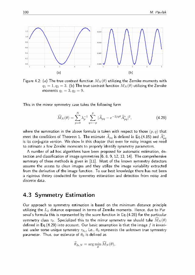
Hence, in practice one has to choose N large enough such that the sum de�ningMN (θ) contains nonzero Apq's for which the condition given in Theorem 1 on theangular repetition q holds. Figure 4.2 illustrates the result described in Theorem 1for an image being mirror symmetric with respect to θ0 = π. The contrast functionMN (θ) is depicted utilizing the terms with q1 = 1, q2 = 3 and q1 = 3, q2 = 9. Theunique global minimum of MN (θ) at θ0 in the former case is clearly seen. This is notthe case in the latter case.The contrast function de�ned in Eq.(4.23) cannot be evaluated since we can only use

the estimated Zernike moments de�ned in Eq.(4.15). Hence, the empirical counterpartof MN (θ) can be de�ned as follows

MN (θ) =

N∑p=0

λ−1p

p∑q=−p

|Apq(f)− Apq(τθf)|2. (4.28)

100 M. Pawlak

1 2 3 4 5

0.0

0.2

0.4

0.6

0.8

1.0

1.2

(a)

1 2 3 4 5

0.000

0.005

0.010

0.015

(b)

Figure 4.2: (a) The true contrast function MN (θ) utilizing the Zernike moments withq1 = 1, q2 = 3. (b) The true contrast functionMN (θ) utilizing the Zernikemoments q1 = 3, q2 = 9.

This in the mirror symmetry case takes the following form

MN (θ) =

N∑p=0

λ−1p

p∑q=−p

|Apq − e−2jqθA∗pq|2, (4.29)

where the summation in the above formula is taken with respect to those (p, q) that

meet the conditions of Theorem 1. The estimate Apq is de�ned in Eq.(4.15) and A∗pqis its conjugate version. We show in this chapter that even for noisy images we needto estimate a few Zernike moments to properly identify symmetry parameters.

A number of ad hoc algorithms have been proposed for automatic estimation, de-tection and classi�cation of image symmetries [6, 8, 9, 12, 13, 14]. The comprehensivesummary of these methods is given in [11]. Most of the known symmetry detectorsassume the access to clean images and they utilize the image variability extractedfrom the derivative of the image function. To our best knowledge there has not beena rigorous theory conducted for symmetry estimation and detection from noisy anddiscrete data.

4.3 Symmetry Estimation

Our approach to symmetry estimation is based on the minimum distance principleutilizing the L2 distance expressed in terms of Zernike moments. Hence, due to Par-seval's formula this is represented by the score function in Eq.(4.28) for the particular

symmetry class τθ. Specialized this to the mirror symmetry we should take MN (θ)de�ned in Eq.(4.29) into account. Our basic assumption is that the image f is invari-ant under some unique symmetry τθ0 , i.e., θ0 represents the unknown true symmetryparameter. Thus, our estimate of θ0 is de�ned as

θ∆,N = arg minθMN (θ),


where we write θ∆,N to emphasize the dependence of the estimate on the image reso-lution ∆ and the number of Zernike moments N used to obtain the estimate. For suchde�ned estimate we obtain results that characterize the statistical accuracy of θ∆,N .

This includes the rate at which θ∆,N tends to θ0 and the limit law. The followingtheorems are specialized to the mirror symmetry parameter estimate that minimizesthe score function de�ned in Eq.(4.29) with respect to θ ∈ [0, π).

Theorem 2. Suppose that an image function f is of bounded variation on D. Thenfor su�ciently large N such that the identi�ability condition in Eq.(4.24) holds wehave

θ∆,N = θ0 +OP (∆),

where OP (·) stands for the convergence in probability.

The obtained rate is the optimal one as it is known [19] that the best rate for parame-ter estimation is the square root of the sample size. This is the case here since ∆ is oforder 1/n and n2 is the sample size. Also it is worth noting that our situation does notbelong to the standard parameter estimation problem as we estimate θ0 without anyknowledge of the underlying image f(x, y). Such problems are referred to as semi-parametric, see [19] for the basic theory of semiparametric inference. Furthermore,the selection of N is not critical as we only need N that should de�ne the uniquenessproperty described in Theorem 1. This should be contrasted with the choice of N forimage reconstruction, see Eq.(4.16) and Eq.(4.17).

Next, we establish asymptotic normality for θ∆,N . This requires a more restrictiveclass of image functions.

Theorem 3. Let the conditions of Theorem 2 be satis�ed. Suppose that f is Lipschitzcontinuous. Then, we have

∆−1(θ∆,N − θ0)L→ N

(0,

8σ2ε

M(2)N (θ0)

),

where

M(2)N (θ0) = 8

N∑p=0

λ−1p

∑|q|≤p

q2|Apq|2 (4.30)

is the second derivative of MN (θ) at θ = θ0 and N (0, σ2) denotes the normal lawwith mean zero and variance σ2.

The proofs of Theorem 2 and Theorem 3 can be derived from the results establishedin [3, 4].

Theorem 3 can be used to construct a con�dence interval for θ0. To this end, weneed an estimate of the asymptotic variance in the above normal limit. First, we can

estimateM(2)N (θ0) directly by using Eq.(4.30) simply by replacing Apq(f) by Apq. Call

102 M. Pawlak

this estimate M(2)N . Further, we can estimate the noise variance σ2

ε by

σ2ε =

1

C(∆)

∑(xi,yj)∈D

1

4

((Zi,j − Zi+1,j

)2+(Zi,j − Zi,j+1

)2), (4.31)

where the sum is taken over all (xi, yj) ∈ D such that (xi+1, yj) ∈ D and (xi, yj+1) ∈D, and C(∆) is the number of terms in this restricted sum. One can show that if f isLipschitz continuous, then σ2

ε − σ2ε = OP

(∆). Using these estimates, we obtain the

following con�dence interval with nominal level α for θ0[θ∆,N − q1−α ·

2√

2σε∆

(M(2)N )1/2

, θ∆,N + q1−α ·2√

2σε∆

(M(2)N )1/2

], (4.32)

where q1−α is the 1− α-quantile of the standard normal distribution.

Remark 1. If in Theorem 3 we only assume that the image f is a function of boundedvariation, then the bias is also of order ∆, and we get an asymptotic o�set, i.e., thelimiting normal law with non-zero mean.

Remark 2. If the image f is not re�ection invariant, the estimator θ∆,N may stillconverge to a certain parameter value θ∗, which is determined by minimizing theL2-distance ‖f − τmθ f‖2. Then f = (f + τmθ∗f)/2 is the best re�ection-symmetric ap-proximation (in the L2 sense) to the original image f . The following empirical versionof f

fN (x, y) =fN (x, y) + τm

θ∆,NfN (x, y)

2

can serve as an estimate of the optimal symmetric version of f . Furthermore, the dis-tance ‖fN − fN‖ can be used to form an empirical measure of the degree of symmetryof non-symmetric f .

Remark 3. Suppose that f is re�ection invariant but is also invariant under somerotation. If f is rotationally invariant, then there will be a minimal angle α = 2π/dfor some integer d, under which f is rotationally invariant. If we use the estimatorθ∆,N in such a situation, then one re�ection axis will be between 0 and α, and we

should use the minimizer of MN (θ) in the interval [0, α) rather than in [0, π).

To illustrate the above asymptotic theory let us consider a simple example. Figure4.3a shows the noisy version of the mirror symmetric image of the resolution 50× 50.In Fig.(4.3b) the true contrast functions MN (θ) and its estimate MN (θ) for N = 7

are depicted. A global minimum of MN (θ) de�nes the estimate θ∆,N .Figure 4.4a shows the noisy version of the image being not re�ection symmetric.

In Fig.(4.4b) the contrast functions MN (θ) and MN (θ) for N = 7 are depicted. The

minimum of MN (θ) gives the re�ection axis angle θ∆,N that de�nes an estimate ofthe best symmetric approximation of the image. This optimal symmetric image isestimated by (fN + τm

θ∆,NfN )/2 and is shown in Fig.(4.4c), see Remark 2. In turn, in


(a)

MN(θ)

θ

(b)

Figure 4.3: (a) Re�ection symmetric noisy image, (b) The contrast functions MN (θ)

(solid curve) and MN (θ) (dashed line) for N = 7.

Fig.(4.5) we show the true (in black) and estimated (in red) axes of mirror symmetryof the image depicted in Fig.(4.1).

(a)

θ

MN(θ)

(b) (c)

Figure 4.4: (a) A noisy image that is not re�ection symmetric, (b) The contrast func-

tions MN (θ) (solid curve) and MN (θ) (dashed line) for N = 7, (c) Anestimate of the best symmetric approximation of the image.

4.4 Symmetry Detection

The aforementioned estimation problem assumes that the image f is invariant undersome unique known symmetry, i.e., that there is θ0 ∈ Θ such that f = τθ0f . In thedetection problem our goal is to test the hypothesis on the symmetry class, i.e., wewish to verify

H0 : f = τθ0f (4.33)

for some θ0 ∈ Θ, against the alternative

Ha : f 6= τθf (4.34)

104 M. Pawlak

Figure 4.5: The true (in black) and estimated (in red) axes of mirror symmetry of theimage depicted in Fig.(4.1)

for all θ ∈ Θ. The test statistic for verifying H0 is based again on the concept of theL2 minimum distance principle and has the generic form

TN (∆) =‖ fN − τθ∆,NfN ‖2, (4.35)

where θ∆,N is the above introduced estimate obtained under the null hypothesis H0.

The minimum distance property of θ∆,N suggests the alternative form of TN , i.e.,

TN (∆) = minθ∈Θ‖ fN − τθfN ‖2 . (4.36)

This statistic only needs the numerical minimization with respect to a single variableθ. The examined detectors are of the form: reject H0 if TN (∆) > c, where c is aconstant controlling the false rejection rate.Let us begin with the problem of testing the hypothesis of mirror symmetry. Since

the minimum L2-distance approach is invariant for the true value of the re�ection angleθ0 we may consider, without loss of generality, the vertical re�ection τmπ/2f(x, y) =

f(−x, y). We will denote this symmetry brie�y as τf = f . In view of Eq.(4.18)we have Apq(τf) = (−1)|q|A∗pq(f). Now consider the hypothesis that f is invariantunder τ , i.e., H0 : f = τf which can be expressed in terms of Zernike coe�cients asApq(f) = (−1)|q|A∗pq(f). Hence, due to Parseval's formula the test statistic de�nedin Eq.(4.35) is given by

TN (∆) =

N∑p=0

p∑q=−p

λ−1p

∣∣Apq − (−1)|q|A∗pq∣∣2.

The following result presents the limit law for statistic TN (∆) under the hypothesis H0

as well as under �xed alternatives. Let C2(D) denote a class of functions possessingtwo continuous derivatives on D.


Theorem 4. Under the hypothesis H0 : f = τf , if ∆ → 0, N → ∞ such that∆N7 → 0, we have

TN (∆)− σ2ε∆2a(N)

∆2√a(N)

L→ N (0, 8σ4ε), (4.37)

where a(N) = (N + 1)(N + 2).Under a �xed alternative Ha : f 6= τf , suppose that f ∈ C2(D). If ∆N5 → ∞ andN3/2∆γ−1 → 0, where γ = 285/208 controls the geometric error [17], we have

∆−1(TN (∆)− ‖f − τf‖2

) L→ N (0, 16σ2ε‖f − τf‖2). (4.38)

It is worth noting that di�erent rates appear under the hypothesis (fast rate) inEq.(4.37) and under �xed alternatives (slow rate) in Eq.(4.38). This takes place sinceTN (∆) is (under the hypothesis) a quadratic statistic [5], but under a �xed alternativean additional linear term arises which dominates the asymptotic. Theorem 4 can beused to construct an asymptotic level α test for verifying the hypothesis H0. Indeed,�xing the Type I detection probability P{TN (∆) > c|H0} to the value α yields thefollowing asymptotic choice of the control limit c

cα = 2q1−α∆2√

2a(N)σ2ε + ∆2a(N)σ2

ε ,

where σ2ε is an estimate of σ2

ε , see Eq.(4.31) and the truncation parameter N can bespeci�ed as N = ∆−α, where 0 < α < 1/7. Hence, H0 is rejected if TN (∆) > cα.The result of Theorem 4 also reveals that under the alternative

TN (∆)→‖ f − τf ‖2 (P ) (4.39)

as ∆→ 0. Consequently, we readily obtain that N5∆TN (∆)→∞ (P ) which impliesthe following consistency result.

Theorem 5. Let Ha : f 6= τf for f ∈ C2(D) hold. If ∆N5 →∞ and N3/2∆γ−1 →0, then as ∆→ 0

P{N5∆TN (∆) > c|Ha

}→ 1 (4.40)

for any positive constant c > 0.

Hence, the properly normalized decision statistic TN (∆) leads to the testing techniquethat is able to detect that the null hypothesis is false with the probability approachingto one, i.e., the power of the test tends to one.Furthermore, let us note that contrary to the symmetry estimation problem the

symmetry detection requires the optimal choice of the truncation parameter N . Thecondition ∆N7 → 0, used under the hypothesis, is rather restrictive, and is due to theonly approximate orthogonality of the discretized Zernike polynomials. This conditioncan be relaxed if we assume a more accurate orthogonal design. In fact, if we haveexact discrete orthogonality, then ∆N2 → 0 is su�cient for Eq.(4.37) to hold. Undera �xed alternative, the condition N3/2∆γ−1 → 0 is equivalent to N4+β∆ → 0,β = 0.0519 . . ., so that this condition and N5∆→∞ can be ful�lled simultaneously.

106 M. Pawlak

Analogous derivations can be carried out for testing d-fold rotation symmetry. Ex-plicit results can be obtained for d = 2 and d = 4. The remaining cases need someinterpolation procedures since the discrete grid points {(xi, yj)} are no longer invariantunder τ r2π/d for arbitrary value of d.

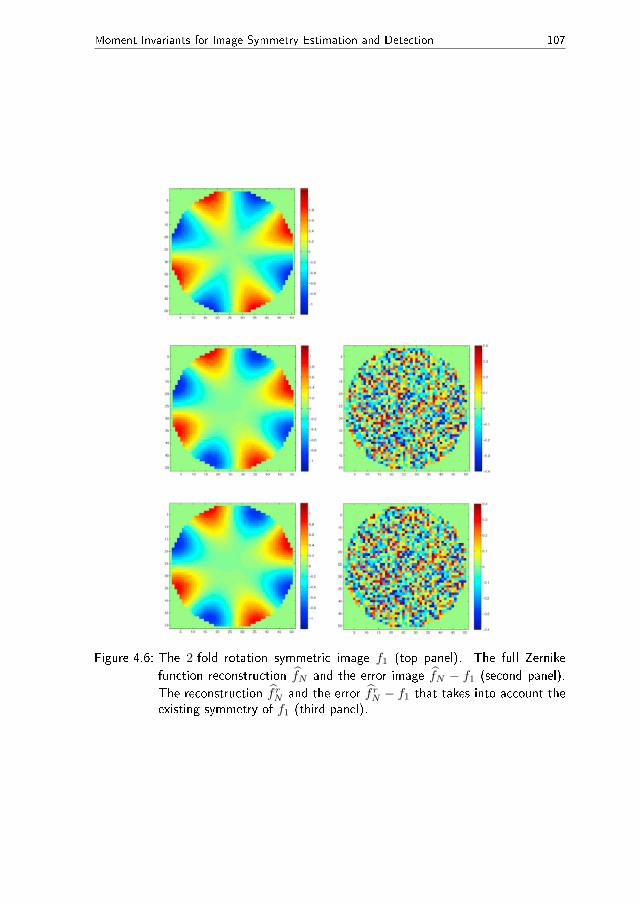
To illustrate this case let us consider an example of the 2-fold rotation symmetricimage f1 shown in Fig.(4.6) (top row). The second row in Fig.(4.6) depicts the

reconstruction fN and the corresponding error image fN − f1. The reconstructionfN here is based on the complete Zernike function expansion that ignores the factthat the image was detected to be symmetric. On the other hand, the third row inFig.(4.6) shows the reconstruction frN and the error frN − f1 that takes into accountthe existing symmetry of f1. In fact, under the 2-fold rotation symmetry we havethat the Zernike moments Apq = 0 for all q being odd. Hence, the reconstruction

frN shown in the third row of Fig.(4.6) is using only Zernike functions with even q. Itis seen that both reconstructions reveal comparable errors, with the preferable visualquality of the symmetry preserving reconstruction frN .

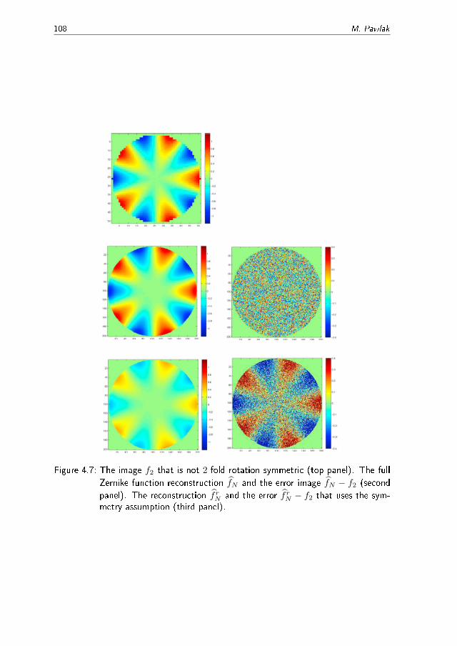
Analogous experiments have been repeated for the not 2-fold rotation symmetricimage f2 depicted in the top panel of Fig.(4.7). The second row of Fig.(4.7) shows

the full Zernike function reconstruction fN and the corresponding error image fN −f2. On the other hand, the third row in Fig.(4.7) shows the reconstruction frN and

the error frN − f2 that falsely assumes that f2 is 2-fold rotation symmetric. Thedramatic increase of the reconstruction error is clearly seen. Hence, either acceptingor rejecting the hypothesis of the image symmetry has an important in�uence on itsvisual perception and recognition.

The case d = ∞ (testing radiality) is of special interest and can be examinedby observing that if the image f is radial, i.e., f(ρ, ϕ) = g(ρ), then we have thatApq(f) = 0 for all q 6= 0. Moreover,

Ap0(f) = 2π

ˆ 1

0

g(ρ)Pp/2(2ρ2 − 1)ρdρ,

where Ps(x) is the Legendre polynomial of order s. This allows us to form the ap-propriate nonparametric test for the image radiality with the power tending to one as∆→ 0, see [16].

It is rare in practise to pose a null hypothesis that the veri�ed not observed image isexactly symmetric. Thus, the exact symmetry hypothesis is replaced by the followingapproximate symmetry requirement

Hδ0 : ‖f − τθ0f‖ ≤ δ (4.41)

with the alternative hypothesis as

Hδa : ‖f − τθ0f‖ > δ, (4.42)

where δ is the assumed degree of image symmetry. This type of hypothesis can beincorporated into our previous scheme by rejecting Hδ

0 if TN (∆)− δ > cα.


Figure 4.6: The 2-fold rotation symmetric image f1 (top panel). The full Zernike

function reconstruction fN and the error image fN − f1 (second panel).

The reconstruction frN and the error frN − f1 that takes into account theexisting symmetry of f1 (third panel).

108 M. Pawlak

Figure 4.7: The image f2 that is not 2-fold rotation symmetric (top panel). The full

Zernike function reconstruction fN and the error image fN − f2 (second

panel). The reconstruction frN and the error frN − f2 that uses the sym-metry assumption (third panel).


4.5 Concluding Remarks

In this chapter, we give the uni�ed minimum L2-distance radial moments based ap-proach for statistical assessing the image symmetry. The problem of symmetry esti-mation can be regarded as a semiparametric estimation problem, with θ as the targetparameter, and the image function as a nonparametric nuisance component [19]. Fur-ther results may include the statistical assessment of imperfect symmetries, symmetriesthat only hold locally and detection and estimation of joint symmetries. In particular,the problem of detection and estimation of symmetry for blurred images is of the greatinterest, i.e., when the observation model in Eq.(4.5) is replaced by

Zi,j =

¨D

K(xi − x, yj − y)f(x, y)dxdy + εi,j ,

where K(x, y) is the point-spread function of the given imaging system. Such a caseplays important role in confocal microscopy and medical imaging [3, 4].Further extensions may also include 3-D imaging where a number of basic symmetry

classes is much larger than in the 2-D case.

References

[1] A.B. Bhatia and E. Wolf. On the circle polynomials of Zernike and relatedorthogonal sets. In Mathematical Proceedings of the Cambridge PhilosophicalSociety, volume 50, 1954.

[2] M. Birke, H. Dette, and K. Stahljans. Testing symmetry of nonparametric bi-variate regression function. Journal of Nonparametric Statistics, 23(2):547�565,2011.

[3] N. Bissantz, H. Holzmann, and M. Pawlak. Testing for image symmetries-withapplication to confocal microscopy. IEEE Transactions on Information Theory,55(4):1841�1855, 2009.

[4] N. Bissantz, H. Holzmann, and M. Pawlak. Improving PSF calibration in confocalmicroscopic imaging - estimating and exploiting bilateral symmetry. Annals ofApplied Statistics, 4(4):1871�1891, 2010.

[5] P. de Jong. A central limit theorem for generalized quadratic forms. ProbabilityTheory and Related Fields, 75(2):261�277, 1987.

[6] S. Derrode and F. Ghorbel. Shape analysis and symmetry detection in gray-level objects using the analytical Fourier-Mellin representation. Signal Processing,84(1):25�39, 2004.

[7] J. Flusser, T. Suk, and B. Zitova. Moments and Moment Invariants in PatternRecognition. Wiley, Chichester, 2009.

[8] Y. Keller and Y. Shkolnisky. A signal processing approach to symmetry detection.IEEE Transactions on Image Processing, 15(8):2198�2207, 2006.

[9] W.Y. Kim and Y.S. Kim. Robust rotation angle estimator. IEEE Transactions onPattern Analysis and Machine Intelligence, 21(8):768�773, 1999.

[10] S.X. Liao and M. Pawlak. On the accuracy of Zernike moments for image analysis.IEEE Transactions on Pattern Analysis and Machine Intelligence, 20(12):1358�1364, 1998.

110 M. Pawlak

[11] Y. Liu, H. Hel-Or, C.S. Kaplan, and L. van Gool. Computational Symmetry inComputer Vision and Computer Graphics. Now Publishers, Boston, 2010.

[12] G. Loy and A. Zelinsky. Fast radial symmetry for detecting points of interest.IEEE Transactions on Pattern Analysis and Machine Intelligence, 25(8):959�973,2003.

[13] L. Lucchese. Frequency domain classi�cation of cyclic and dihedral symmetriesof �nite 2-d patterns. Pattern Recognition, 37(12):2263�2280, 2004.

[14] G. Marola. On the detection of the axes of symmetry of symmetric and almostsymmetric planar images. IEEE Transactions on Pattern Analysis and MachineIntelligence, 11(1):104�108, 1989.

[15] R. Mukundan and K.R. Ramakrishnan. Moment Functions in Image Analysis:Theory and Appplications. World Scienti�c, Singapore, 1998.

[16] M. Pawlak. Image Analysis by Moments: Reconstruction and Computa-tional Aspects. Wroclaw University of Technology Press, Wroclaw, 2006.http://www.dbc.wroc.pl/dlibra/doccontent?id=1432&from=&dirids=1.

[17] M. Pawlak and S.X. Liao. On the recovery of a function on a circular domain.IEEE Transactions on Information Theory, 48(10):2736�2753, 2002.

[18] J. Rosen. Symmetry in Science: An Introduction to the General Theory. Springer-Verlag, New York, 1995.

[19] A. W. van der Vaart. Asymptotic Statistics. Cambridge University Press, Cam-bridge, 1998.

[20] Q. Wang, O. Ronneberger, and H. Burkhardt. Rotational invariance based onFourier analysis in polar and spherical coordinates. IEEE Transactions on PatternAnalysis and Machine Intelligence, 31(9):1715�1722, 2009.

Chapter 4: Moment Invariants for Image Symmetry Estimation...

Documents

Transcript of Chapter 4: Moment Invariants for Image Symmetry Estimation...