1

Chapter 3 Models for Transmission Expansion Planning based on Reconfigurable Capacitor Switching

J. McCalley R. Kumar V. Ajjarapu O. Volij H. Liu L.Jin W. Shang Department of Electrical and Computer Engineering Department of Economics

Iowa State University Iowa State University Editor’s summary: 3.1 INTRODUCTION

Transmission expansion planning is the process of deciding how and when to invest in additional transmission facilities. It is complicated under any electric industry structure because resulting decisions can affect any stakeholder owning or operating interconnected facilities and are necessarily driven by predictions of uncertain futures characterized by changes in load and generation, and by potential of component unavailability from forced or scheduled outage. These decisions have significant consequences on the reliability and economy of the future interconnected power system; in addition, they usually involve large capital expenditures and complex regulatory processes, especially if they require obtaining right-of way, and so represent high financial commitment to investors. Previous to deregulation when electric utilities were vertically integrated, overseeing generation, transmission, and distribution under one management structure, the necessary coordination between the highly interdependent functions was carried out in an intentionally integrated fashion, often involving the same people, targeting the objectives of the organization’s management to whom the analysts and decision-makers reported. Transmission enhancements that affected multiple utilities were handled through bilateral coordination or through well-structured coordinating bodies. The utility paid for transmission upgrades and recovered regulatory-approved costs through customer rates. The most significant uncertainties faced by planners were load growth and component forced outage (due to a fault or failure), uncertainties for which historical data can be used in deriving associated probability distributions.

Under deregulation, the number of organizations involved in generation planning and transmission planning is significantly increased, each with their own objectives. Generation is planned by a multiplicity of companies seeking to maximize their individual profits through energy sales, while transmission is planned by transmission owners seeking to maximize their profits through transmission services, all overseen and coordinated by a centralized authority seeking to ensure grid reliability and market efficiency. The increased number of stakeholders requires procedures for coordinating among them the necessary analyses, decisions, and financial implications; in addition, it motivates the need for incentives so that organizations perceive transmission investment and ownership to be attractive. The number and nature of uncertainties have increased as well [1]. In addition to load uncertainty and component forced outages, planners must account for uncertainty in generation and transmission installation, in generation commitment and dispatch schedules, in wheeling (point-to-point power transactions), and in component economic outages due to financially-motivated decision on the part of the component owner.

Although electricity markets have been operating in the U.S. since the early 1990’s, it has only been recent that planning procedures and investment incentives have begun to mature. As a result, transmission investment has been inhibited during the early deregulation years, as indicated in Fig. 1 [2], which compares U.S. annual average growth rates of transmission and load during three periods of time from 1982 to 2012, and Fig. 2 [3], which compares U.S. investment trends in distribution, transmission, and generation from 1925 to 2020. The figures show transmission growth and investment at its lowest point during the period 1992-2002.

2

Fig. 1: Annual avg. growth rates of transmission, load [2] Fig. 2: Capital investment as percentage of revenues [3]

From an engineering perspective, there are four options for expanding transmission: (1) build new transmission circuits, (2) upgrade old ones, (3) build new generation at strategic locations, and (4) introduce additional control capability. Although all of these continue to exist as options, options (1)-(3) are more capital-intensive than option (4); right-of-way acquisition can sometimes prohibit option (1), and option (3) as a transmission solution is almost always considered secondary to energy market profitability. Option (4), control, although not always viable, is attractive when it is viable since it is relatively inexpensive, requires no right of way, and when not part of generation facilities, affects energy market operation only through the intended transmission expansion.

Although considerable work has been done in planning transmission in the sense of options (1)-(3), there has been relatively little effort towards planning transmission control options in the sense of option (4), yet the ability to consider these devices in the planning process is a clear need to the industry [4, 5, 6, 7]. Our interest therefore focuses on designing systematic control system planning algorithms. There are 4 types of control technologies that exist today: generation controls, power-electronic based transmission control, system protection schemes (SPS), and mechanically switched shunt and series devices (capacitors, reactors, and phase-shifters). Of these, the first two exert continuous feedback control action; the third and fourth exert discrete open-loop control action. Thus, power system control is hybrid [8, 9] in that it consists of continuous and discrete control. Since power systems are already hybrid, and since good solutions may also be hybrid, assessment of control alternatives for expanding transmission must include procedures for gauging cost and effectiveness of hybrid control schemes. Our emphasis is on the most promising and least expensive of the discrete control options, series and shunt capacitor switching; the aim is to provide flexible and inexpensive transmission expansion via reconfigurable switching of these controls in response to network disturbances that can occur.

In this chapter, we target planning methods and investment implications for enhancing transmission via discrete control. In Section 3.2, we summarize current market-based planning procedures because, owing to their recent development, the literature is relatively sparse on this topic; in addition, this summary illuminates the environment in which the methods described in this paper are intended for use. Section 3.3 describes and clarifies one particularly complex planning issue that is at the heart of our work: transmission limits. Section 3.4 provides engineering models capable of identifying solutions to planning problems. Section 3.5 analyzes electricity market efficiency under two types of transmission expansion options, new lines and control, resulting in the interesting conclusion that electricity markets allowing only control-based expansion are efficient, whereas markets that allow new transmission lines are not. Section 3.6 concludes.

3.2 PLANNING PROCESSES

A transmission planning study is an economic and engineering analysis of a transmission network to identify problems associated with expected future conditions together with solutions to those problems. Such a study may be motivated by the likely prospect of a single significant network change, e.g., the proposal of a large generation facility. However, it is essential to conduct planning studies periodically to account for normal load growth, retirement of old facilities, and changes in maintenance and operating policies. As a result, minimum planning frequency has generally been yearly, projecting conditions 5-10 years ahead.

3

Order 2000 of the Federal Energy Regulatory Commission (FERC) stipulated that regional transmission organizations (RTOs) have “ultimate responsibility for both transmission planning and expansion within its region” [10]. An RTO is an organization, independent of all generation or transmission owners and load-serving entities, that facilitates electricity transmission on a regional basis with responsibilities for grid reliability and transmission operation. Organizations approved or under consideration by FERC for approval as an RTO are shown in Fig. 3 [11] as the white ovals. Two primary issues for RTO-based planning are coordinating plans of multiple stakeholders and provision of investment incentives including articulation of a cost-recovery path for transmission investors.

Fig. 3: Existing and Proposed RTOs [11]

FERC also issued an important ruling in 2003, called Order 2003 [12], which required public utilities to “file revised open access transmission tariffs containing standard generator interconnection procedures and a standard agreement that the Commission is adopting in this order…” These procedures, described in Order 2003, were encapsulated in a diagram contained in an appendix of Order 2003 [13]. Figure 4 provides a simplified version of this diagram.

Fig. 4: Simplified Illustration of FERC’s Interconnection Procedures

4

In the remainder of this section, we describe some aspects of a planning process and cost-recovery approach used by one RTO, PJM Interconnection, based largely on [14,15]. 3.2.1 Engineering analyses and cost responsibilities

Each planning cycle begins with an information gathering stage where RTO engineers solicit information from a full range of stakeholders including independent power producers (IPPs), interconnected transmission owners (ITOs) and transmission developers (TDs) proposing development plans, load serving entities (LSEs), and all regional reliability councils, independent system operators (ISOs), and transmission owners and operators within and adjoining the RTO network. Project queues are developed of proposed generation and transmission projects based on receipt of an interconnection request. Queued projects are assigned one of the following status indicators, in order of study sequence: feasibility study, impact study, facility study, interconnection service agreement (ISA), being built, or built.

A baseline analysis of system reliability is performed by the RTO; this analysis models expected load growth and known transmission and generation projects, but it models development projects in the queue depending on their status. If a project has proceeded to the stage of ‘facility study,’ its associated system upgrades are modeled. If a project has proceeded to the stage of ‘ISA,’ it could be turned on in the basecase, even it has not been built. Power flow, voltage, time-domain (stability), and short-circuit studies are conducted to evaluate the reliability according to applicable criteria and to identify baseline expansion projects necessary to satisfy violated criteria that cause unhedgeable congestion (unhedgeable congestion is described in Section 3.2.3 below).

An initial feasibility study is performed for each interconnection request to provide a rough approximation of the transmission-related costs necessary to accommodate the interconnection in order to enable the developer to make an informed business decision, at which point the developer either drops out of the queue or signs a system impact study agreement. System impact studies are performed for each interconnection request remaining in the queue. System impact studies provide a more detailed assessment of interconnection requirements, revealing necessary enhancements. Such enhancements may include direct connection attachment facilities (required for new generation to “get to the bus”) and/or network reinforcements to mitigate “network impact” effects that the proposed transmission development may have on the power system. Each interconnection project bears the cost responsibility for its own direct connection attachment facilities. The cost responsibility for network reinforcements is allocated among parties based on the percent impact which a given project has on a system element requiring upgrade. In the power flow cost allocation method, upgrade costs are allocated based on each party’s MW impact on the need for the system upgrade, as determined by “distributed slack” power transfer distribution factors [16], defined as the MW impact on a line when transferring 1MW of power from the new generating bus to all the rest of the generating buses. Such an approach is appropriate for cost allocation for new or re-conductored lines, for example. The short-circuit cost allocation method, applicable to upgraded circuit breakers, allocates costs in proportion to the fault level contribution of each proposed IPP. Identified network reinforcement costs, for a given capacity, are highly dependent on location, and developers have strong incentives to identify development locations that minimize these costs.

3.2.2 Cost Recovery for Transmission Owners

In addition to the investment or capital costs, transmission owners also incur ongoing costs due to operations and maintenance, administration, debt amortization, depreciation, and taxes. Transmission cost-recovery of all of these costs is accomplished in three primary ways. • Network integration transmission service charges [17]: Network customers are so designated because they pay a

transmission charge computed as the summation of their daily peak load multiplied by the annual network integration transmission service rate (in the zone in which the load is located) divided by 365. Typical service charges at the time of this writing range from 11,020-32,114 $/MW-year in the PJM area. Each transmission owner computes these service rates based on their annual transmission revenue requirements, which range from $12 million to $1.6 billion in the PJM area.

• Point-to-point transmission service charges [17]: Point-to-point customers obtain transmission service between a point of delivery to a point of receipt. Service may be firm (curtailed last) or non-firm (curtailed first); the calculation procedure for service charges, which is the same in both cases (but non-firm rates are less), is to multiply the capacity reserved by the rate. The published yearly firm rate at the time of this writing is

5

$18.88/kw-year. Total firm charges are allocated to the transmission owners in proportion to their annual revenue requirements. Total non-firm charges are allocated to the firm point-to-point and network transmission customers based on percentage shares of their firm and network demand charges, respectively.

• Auction revenue rights (ARRs) [18]: ARRs are entitlements allocated annually to firm transmission service customers (which can include transmission owners) that entitle the holder to receive an allocation of the revenues from the annual FTR auction. FTRs are financial instruments that entitle the holder to rebates of congestion charges paid by firm transmission service customers. So transmission owners can purchase ARRs which give them the right to receive compensation from the proceeds of FTR sales. FTRs are sold to market participants to hedge against the possibility of paying congestion charges when flows on a transmission path exceed the path limit, and generation must be uneconomically dispatched to avoid overload. That is, whenever congestion exists on the transmission system between sink and source points specified in a particular FTR, such that the locational marginal price (LMP) at the sink point (point of delivery) is higher than the LMP at the source point (point of receipt), the holder of that FTR receives a credit equal to the MW reservation specified in the FTR and the difference between the LMPs at the two specified points. (We assume that readers are familiar with LMPs, which are fundamental to understanding electricity markets. Basic treatment of LMPs may be found in [19, 20, 21].)

3.2.3 Economically motivated expansion

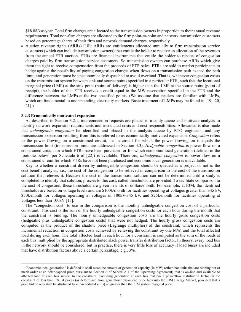
As described in Section 3.2.1, interconnection requests are placed in a study queue and motivate analysis to identify network expansion requirements and associated costs and cost responsibilities. Allowance is also made that unhedgeable congestion be identified and placed in the analysis queue by RTO engineers, and any transmission expansion resulting from this is referred to as economically motivated expansion. Congestion refers to the power flowing on a constrained circuit, i.e., a circuit for which the power flowing on it equals the transmission limit (transmission limits are addressed in Section 3.3). Hedgeable congestion is power flow on a constrained circuit for which FTRs have been purchased or for which economic local generation (defined in the footnote below1 per Schedule 6 of [22]) is available. Therefore, unhedgeable congestion is power flow on a constrained circuit for which FTRs have not been purchased and economic local generation is unavailable.

Key to whether a constraint driven by unhedgeable congestion should be queued as a project or not is the cost-benefit analysis, i.e., the cost of the congestion to be relieved in comparison to the cost of the transmission solution that relieves it. Because the cost of the transmission solution can not be determined until a study is completed to identify that solution, proxies to this cost, called thresholds, are provided. To facilitate comparison to the cost of congestion, these thresholds are given in units of dollars/month. For example, at PJM, the identified thresholds are based on voltage levels and are $100k/month for facilities operating at voltages greater than 345 kV, $50k/month for voltages operating at voltages of 100kV-345 kV, and $25k/month for facilities operating at voltages less than 100kV [15].

The “congestion cost” to use in the comparison is the monthly unhedgeable congestion cost of a particular constraint. This cost is the sum of the hourly unhedgeable congestion costs for each hour during the month that the constraint is binding. The hourly unhedgeable congestion costs are the hourly gross congestion costs (hedgeable plus unhedgeable congestion costs) that were not hedged. The hourly gross congestion costs are computed as the product of the shadow price (Lagrange multiplier) of the constraint, which represents the incremental reduction in congestion costs achieved by relieving the constraint by one MW, and the total affected load during each hour. The total affected load in each hour for a constraint is computed as the sum of the loads at each bus multiplied by the appropriate distributed slack power transfer distribution factor. In theory, every load bus in the network should be considered, but in practice, there is very little loss of accuracy if load buses are included that have distribution factors above a certain percentage, e.g., 3%.

1 “Economic local generation” is defined in shall mean the amount of generation capacity (in MW) (other than units that are running out of merit order at an offer-capped price pursuant to Section 6 of Schedule 1 of the Operating Agreement) that is on-line and available to affected load at each bus subject to the constraint, excluding generation at each bus that has a powerflow distribution factor on the constraint of less than 3%, at prices (as determined from generators’ day-ahead price bids into the PJM Energy Market, provided that a price bid of zero shall be attributed to self-scheduled units) no greater than the PJM system marginal price.

6

Thresholds are the first step to identifying recommended economically motivated expansion. The identification of a path for which unhedgeable congestion exceeds threshold means that a market window has opened and market participants have the ability to propose projects through the queues for relieving the constraint. If no market solution to the congestion is present after one year, then a more detailed cost-benefit analysis is performed. 3.2.4 Further reading

This section has provided a highly condensed view of existing planning processes for electric transmission systems as reported by PJM. Another reference useful in study of the PJM implementation includes [23]. Although other implementations of RTO-based planning processes share some similarities with that of PJM’s, significant differences exist. Some other implementations at the time of this writing include that of the New York ISO [24], ISO-New England [25], Cal-ISO [26, 27], the Electric Reliability Council of Texas (ERCOT) [28, 29], and the Midwest ISO [30]. A different but equally important view on transmission expansion, from a pure transmission company, is provided in Section I of [31] and [32]. Some additional recommended reading includes [33] which provides historical context and reviews some of the other implementations and [34] which also surveys some of the other implementations. A book on related policy and strategy was also recently published [35]. 3.3 TRANSMISSION LIMITS

The North American Electric Reliability Council (NERC), maintains an extensive set of planning standards [ 36 ] that address system reliability, system modeling data requirements, system protection and control, and system restoration. These standards require that under normal operating conditions, also called pre-contingency conditions, Level A performance requirements be met such as circuit loadings are within continuous ratings and voltage magnitudes lie within a specified range, e.g., 0.97-1.05 pu. In addition, reliability standards require that under contingency conditions, specified disturbance-performance criteria are met. A fundamental part of the reliability standards is the disturbance-performance table. This table is based on the planning philosophy that a higher level of performance (or lower level of severity) is required for disturbances having a higher occurrence likelihood. Typical disturbance -performance criteria are shown in Table 1. This table is similar in principle to NERC’s table [37], where, for example, performance Level B requires that loss of a single element (an N-1 contingency) result in performance where: (a) transient criteria require that voltage dips may not exceed 25% of pre-contingency levels for any time, they may not exceed 20% for more than 20 cycles (0.333 sec), and frequency transients may not exceed 59.6 hz for more than 6 cycles, and (b) post-transient criteria require that voltage deviations remain within 5% of pre-contingency voltages, and all circuit loadings within their applicable ratings. Level C criteria applies to the less likely loss of two components (an N-2 contingency), but its performance criteria is less restrictive. Level D applies to very rare events with no explicit performance criteria specified, leaving the engineer to make a judgment. A voltage instability criterion is usually applied in planning studies, but to maintain simplicity, such a criterion is not indicated in Table 1.

Key to understanding power system flow limitations is the fact that limits on operating conditions (such as flows) can be imposed by violation of either Level A criteria or the contingency-driven Levels B or C criteria. In the case of Level A violation, transmission enhancements identified to relieve the violation must operate under normal conditions. In the case of Level B or C violation, transmission enhancements identified to relieve the violation (which is a post-contingency violation) need operate only following the contingency; thus, they may be

Table 1: Example of Typical Disturbance-Performance Criteria

Performance Requirements

Transient Criteria Post-transient criteria

Disturbance

Perf. Level

Transient voltage dip criteria, ΔV1

Minimum transient frequency

Post transient voltage dev,ΔV2

Loading within emergency ratings

SLG fault or 3F fault w/loss of 1 generator or 1 circuit or DC monopole

B - max V Dip - 25% - max duration of V dip exceeding 20% is 20 cycles

max duration of freq<59.6 hz is 6 cycles

5% Yes

SLG w/ or w/o delayed clearing or 3F fault w/loss of 2 generators or 2 circuits or DC bipole

C - max V Dip - 30% - max duration of V dip exceeding 20% is 40 cycles

max duration of freq<59.0 hz is 6 cycles

10% Yes

Extreme events such as 3F fault with delayed clearing w/loss of 2 or more components

D Evaluate for risks and consequences

7

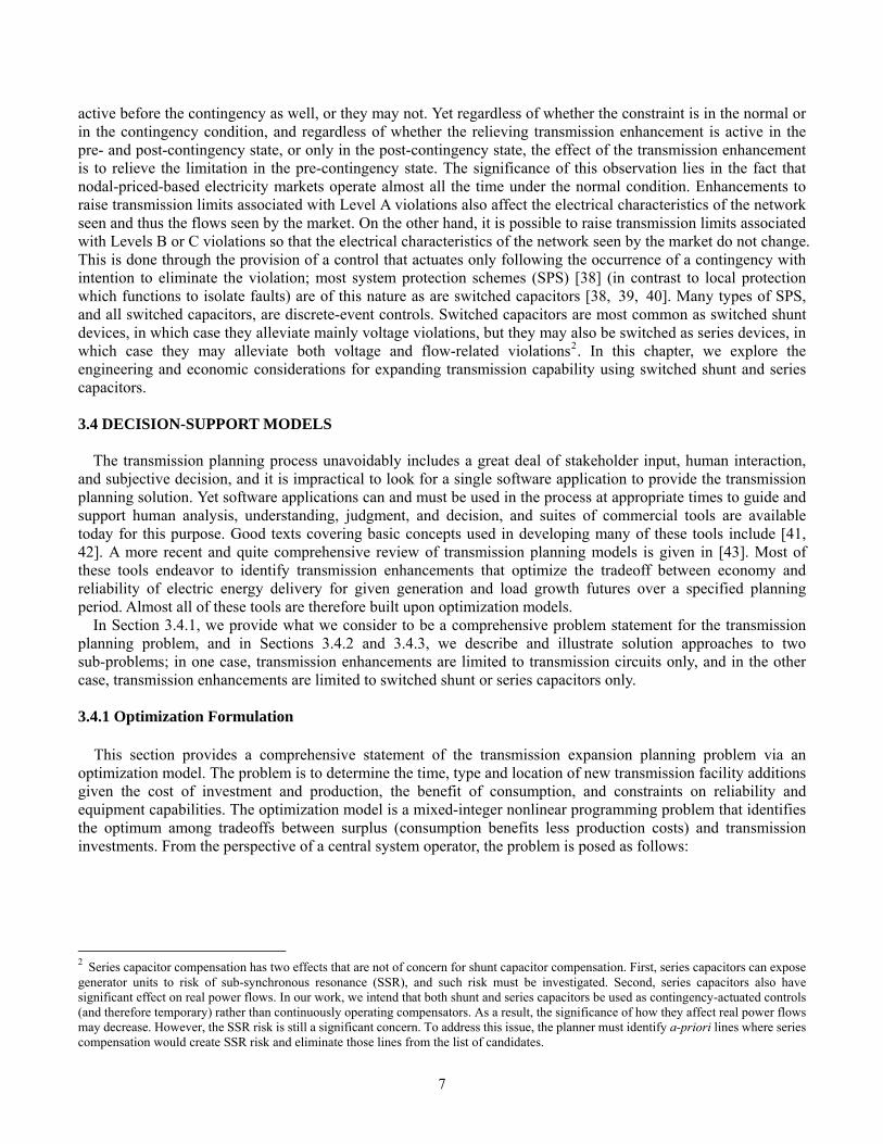
active before the contingency as well, or they may not. Yet regardless of whether the constraint is in the normal or in the contingency condition, and regardless of whether the relieving transmission enhancement is active in the pre- and post-contingency state, or only in the post-contingency state, the effect of the transmission enhancement is to relieve the limitation in the pre-contingency state. The significance of this observation lies in the fact that nodal-priced-based electricity markets operate almost all the time under the normal condition. Enhancements to raise transmission limits associated with Level A violations also affect the electrical characteristics of the network seen and thus the flows seen by the market. On the other hand, it is possible to raise transmission limits associated with Levels B or C violations so that the electrical characteristics of the network seen by the market do not change. This is done through the provision of a control that actuates only following the occurrence of a contingency with intention to eliminate the violation; most system protection schemes (SPS) [38] (in contrast to local protection which functions to isolate faults) are of this nature as are switched capacitors [38, 39, 40]. Many types of SPS, and all switched capacitors, are discrete-event controls. Switched capacitors are most common as switched shunt devices, in which case they alleviate mainly voltage violations, but they may also be switched as series devices, in which case they may alleviate both voltage and flow-related violations2. In this chapter, we explore the engineering and economic considerations for expanding transmission capability using switched shunt and series capacitors. 3.4 DECISION-SUPPORT MODELS

The transmission planning process unavoidably includes a great deal of stakeholder input, human interaction, and subjective decision, and it is impractical to look for a single software application to provide the transmission planning solution. Yet software applications can and must be used in the process at appropriate times to guide and support human analysis, understanding, judgment, and decision, and suites of commercial tools are available today for this purpose. Good texts covering basic concepts used in developing many of these tools include [41, 42]. A more recent and quite comprehensive review of transmission planning models is given in [43]. Most of these tools endeavor to identify transmission enhancements that optimize the tradeoff between economy and reliability of electric energy delivery for given generation and load growth futures over a specified planning period. Almost all of these tools are therefore built upon optimization models.

In Section 3.4.1, we provide what we consider to be a comprehensive problem statement for the transmission planning problem, and in Sections 3.4.2 and 3.4.3, we describe and illustrate solution approaches to two sub-problems; in one case, transmission enhancements are limited to transmission circuits only, and in the other case, transmission enhancements are limited to switched shunt or series capacitors only. 3.4.1 Optimization Formulation

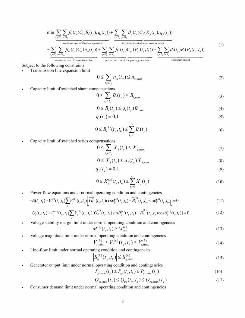
This section provides a comprehensive statement of the transmission expansion planning problem via an optimization model. The problem is to determine the time, type and location of new transmission facility additions given the cost of investment and production, the benefit of consumption, and constraints on reliability and equipment capabilities. The optimization model is a mixed-integer nonlinear programming problem that identifies the optimum among tradeoffs between surplus (consumption benefits less production costs) and transmission investments. From the perspective of a central system operator, the problem is posed as follows:

2 Series capacitor compensation has two effects that are not of concern for shunt capacitor compensation. First, series capacitors can expose generator units to risk of sub-synchronous resonance (SSR), and such risk must be investigated. Second, series capacitors also have significant effect on real power flows. In our work, we intend that both shunt and series capacitors be used as contingency-actuated controls (and therefore temporary) rather than continuously operating compensators. As a result, the significance of how they affect real power flows may decrease. However, the SSR risk is still a significant concern. To address this issue, the planner must identify a-priori lines where series compensation would create SSR risk and eliminate those lines from the list of candidates.

8

1 2

investment cost of shunt compensation investment cost of series compensation

min ( ) ( ( ), ( )) ( ) ( ( ), ( ))

( ) ( ( ))

y y y y

y m

i y i i y i y j y j j y j yt T i t T j

m y m m yt m N

t C B t q t t C X t q t

t C n t

β β

β

∈ ∈Ω ∈ ∈Ω

∈ ∈

+

+

∑ ∑ ∑ ∑

∑

1444442444443 144444424444443

consumer benefitinvestment cost of transmission line production cost of real power generation

( ) ( ( , )) ( ) ( ( , ))y h h g h h l

z y gz gz y h l y l dl y hT t T z N t T l N

t C P t t t R P t tβ β∈ ∈ ∈ ∈

+ −∑ ∑ ∑ ∑ ∑1444424444314444244443 1444442444443

(1)

Subject to the following constraints: • Transmission line expansion limit

,max0 ( )y y

m y mt T

n t n∈

≤ ≤∑ (2)

• Capacity limit of switched shunt compensations

,max0 ( )y y

i y it T

B t B∈

≤ ≤∑ (3)

,max0 ( ) ( )i y i y iB t q t B≤ ≤ (4)

( ) 0,1i yq t = (5)

( )

1

0 ( , ) ( )y

y

tk

i y h i yt

B t t B t=

≤ ≤∑ (6)

• Capacity limit of switched series compensations

,max0 ( )y y

j y jt T

X t X∈

≤ ≤∑ (7)

,max0 ( ) ( )j y j y jX t q t X≤ ≤ (8)

( ) 0,1j yq t = (9)

( )

1

0 ( , ) ( )y

y

tk

j y h j yt

X t t X t=

≤ ≤∑ (10)

• Power flow equations under normal operating condition and contingencies

( ) ( )( ) ( ) ( ) ( )( , ) ( , ) ( , ) ( , )cos ( , ) ( , )sin ( , ) 0k kk k k k

ijiji y h i y h j y h y h ij y h y h ij y hj

P t t V t t V t t G t t t t B t t t tθ θ⎡ ⎤− + + =⎢ ⎥⎣ ⎦∑ (11)

( ) ( )( ) ( ) ( ) ( )( , ) ( , ) ( , )[ ( , )sin ( , ) ( , ) cos ( . )] 0k kk k k k

ijiji y h i y h j y h y h ij y h y h ij y hj

Q t t V t t V t t G t t t t B t t t tθ θ− + − =∑ (12)

• Voltage stability margin limit under normal operating condition and contingencies ( ) ( )

min( , )k ky hM t t M≥ (13)

• Voltage magnitude limit under normal operating condition and contingencies

( ) ( ) ( ),min ,max( , )k k k

i i y h iV V t t V≤ ≤ (14) • Line-flow limit under normal operating condition and contingencies

( ) ( )

,max( , )k kij y h ijS t t S≤ (15)

• Generator output limit under normal operating condition and contingencies ,min ,max( ) ( , ) ( )gz y gz y h gz yP t P t t P t≤ ≤ (16)

,min ,max( ) ( , ) ( )gz y gz y h gz yQ t Q t t Q t≤ ≤ (17) • Consumer demand limit under normal operating condition and contingencies

9

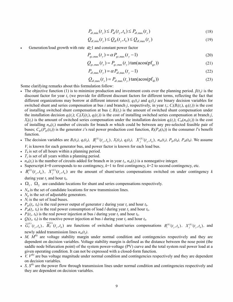
,min ,max( ) ( , ) ( )dl y dl y h dl yP t P t t P t≤ ≤ (18)

,min ,max( ) ( , ) ( )dl y dl y h dl yQ t Q t t Q t≤ ≤ (19)

• Generation/load growth with rate α>1 and constant power factor

,max ,max( ) ( 1)gz y gz yP t P tα= − (20)

,max ,max gz( ) ( ) tan(acos(pf ))gz y gz yQ t P t= (21)

,max ,max( ) ( 1)dl y dl yP t P tα= − (22)

,max ,max dl( ) ( ) tan(acos(pf ))dl y dl yQ t P t= (23) Some clarifying remarks about this formulation follow: • The objective function (1) is to minimize production and investment costs over the planning period. β(ty) is the

discount factor for year ty (we provide for different discount factors for different terms, reflecting the fact that different organizations may borrow at different interest rates); qi(ty) and qj(ty) are binary decision variables for switched shunt and series compensation at bus i and branch j, respectively, in year ty; Ci(Bi(ty), qi(ty)) is the cost of installing switched shunt compensation at bus i; Bi(ty) is the amount of switched shunt compensation under the installation decision qi(ty); Cj(Xj(ty), qj(ty)) is the cost of installing switched series compensation at branch j, Xj(ty) is the amount of switched series compensation under the installation decision qj(ty); Cm(nm(ty)) is the cost of installing nm(ty) number of circuits for branch m which could be between any pre-selected feasible pair of buses; Cgz(Pgz(th)) is the generator z’s real power production cost function, Rl(Pdl(th)) is the consumer l’s benefit function.

• The decision variables are Bi(ty), qi(ty), ( ) ( , )ki y hB t t , Xj(ty), qj(ty), ( ) ( , )k

j y hX t t , nm(ty), Pgz(th), Pdl(th). We assume Vi is known for each generator bus, and power factor is known for each load bus.

• Th is set of all hours within a planning period. • Ty is set of all years within a planning period. • nm(ty) is the number of circuits added for branch m in year ty, nm(ty) is a nonnegative integer. • Superscript k=0 corresponds to no contingency, k=1 to first contingency, k=2 to second contingency, etc. •

( ) ( , )ki y hB t t , ( ) ( , )k

j y hX t t are the amount of shunt/series compensations switched on under contingency k during year ty and hour th.

• 1Ω , 2Ω are candidate locations for shunt and series compensations respectively. • Nm is the set of candidate locations for new transmission lines. • Ng is the set of adjustable generators. • Nl is the set of load buses. • Pgz(ty, th) is the real power output of generator z during year ty and hour th. • Pdl(ty, th) is the real power consumption of load l during year ty and hour th. • Pi(ty, th) is the real power injection at bus i during year ty and hour th. • Qi(ty, th) is the reactive power injection at bus i during year ty and hour th. •

( )( , )

kij y hG t t ,

( )( , )

kij y hB t t are functions of switched shunt/series compensations ( ) ( , )k

i y hB t t , ( ) ( , )kj y hX t t , and

newly added transmission lines nm(ty). • M, M(k) are voltage stability margin under normal condition and contingencies respectively and they are

dependent on decision variables. Voltage stability margin is defined as the distance between the nose point (the saddle node bifurcation point) of the system power-voltage (PV) curve and the total system real power load at a given operating condition. It can not be expressed with a closed-form function.

• V, V(k) are bus voltage magnitude under normal condition and contingencies respectively and they are dependent on decision variables.

• S, S(k) are the power flow through transmission lines under normal condition and contingencies respectively and they are dependent on decision variables.

10

The above formulation requires an optimized network solution together with a full contingency assessment for every hour of the planning period. Although rigorous, computational requirements render such a formulation impractical for large-scale networks. As a result, approximations are typically necessary and can include one or more of the following: • Hours: Analysis in each year may be limited to only representative hours, e.g., typical hours in a day (peak,

off-peak), for typical days (weekdays, weekend days), within a few seasons (summer, winter) to estimate the required attributes over the year.

• Years: Analysis may be limited to only certain years within the planning period; the simplest approximation would study include only the final year.

• Decision variables and objective function: Decision variables may be limited to only those associated with transmission circuits or to only those associated with switched reactive elements.

We consider two cases in the following sections where the hours and years are limited to only one, the peak load hour during the final year. In the first case, described in Section 3.4.2, the decision variables are limited to only those associated with transmission circuits. In the second case, described in Section 3.4.3, the decision variables are limited to only those associated with switched reactive elements. 3.4.2 Planning transmission circuits

The formulation of 3.4.1 reduces to the formulation presented in this section if we restrict our decision variables to just transmission circuits and make the following additional assumptions: • The planning horizon is over Ty periods with the variable t representing a single period so that ty=1,…, Ty. A

period could be a single year, but it may be more appropriate to cover the range of loading conditions that it be quarters (i.e., fall, winter, spring, summer).

• Peak loading conditions are modeled for each period, and it is assumed that these conditions are constant throughout the period.

• Costs of planning and building a new transmission circuit are incurred during the period that it goes into service.

• The consumer utility is assumed to be a constant during each period (i.e., the consumer demand is fixed). • We do not consider contingencies. • The DC power flow model is adopted.

The formulation given in this section is adapted from that given in Section 6.3 of [1]. The objective function of our optimization problem can be formulated as the sum of the aggregate production costs CE and the aggregate transmission circuit investment costs CI in future periods, according to:

1 1 1

( ) ( ) ( ) ( ) ( ) ( )y g y

y y b

T N T

E I z y gz y gz y b y b y b yt z t b N

C C C t C t P t t C t q tβ β= = = ∈

= + = +∑∑ ∑∑ (24)

• βz(ty) is the discount factor of real power production cost for period ty, βb(ty) is the discount factor of transmission circuit investment cost for period ty.

• Cgz(ty) is average cost of producing 1 per-unit power at node z during period ty. • Pgz(ty) is the generation level for unit z at period ty loading conditions. • Nb is the set of candidate circuits. • Cb(ty) is the investment cost of a circuit in branch m during period ty. • qb(ty) is an integer 0 or 1. It is 1 if circuit b∈Nb is put in service during period ty, and 0 otherwise. In other

words, each candidate transmission circuit is associated with a binary decision variable. The equality constraints that we need are those which will force the solution to satisfy electrical laws associated

with how power flows in the network. This is accomplished by enforcing the DC power flow equations. PPA B

T = (25) θ××= )( ADPB (26)

where A is the network node-arc incidence matrix and D is a diagonal matrix of negative branch susceptances. First set corresponding to eq. (25) is as follows:

11

: [ ] : [ ]

, 1,...( )

, 1,...di gi g

b bb B b k b E b k di g

P P i NP P

P i N N= =

− =⎧− + = ⎨ = +⎩

∑ ∑ (27)

The second set corresponding to eq. (26) is as follows. For existing branches ( eb N∈ )

( [ ]) ( [ ]) b bB b E b X Pθ θ− = (28)

For candidate branches ( bb N∈ ): ( [ ]) ( [ ]) ( ( ) 1)b b b y bB b E b X P z t G Uθ θ− = + − + (29)

2(1 ( ))b b yU z t G≤ − (30)

0bU > (31) Here, • bP is the flow on branch b if that flow is in the defined direction. • B[b]: This is the node from which branch b begins. • E[b]: This is the node at which branch b ends. • θ(B[b]) is the angle variable at the begin node of branch b. • θ(E[b]) is the angle variable at the end node of branch b. • Pdi is the demand at node i. • Pgi is the generation at bus i (previously defined). • Ng is the total number of generator buses. • N is the total number of buses. • Xb: The branch reactance associated with branch b. • Ne: The set of existing branches. • Nb: The set of candidate branches (previously defined). • Ub is a continuous fictitious variable included in the decision vector. • G is a large constant. zb(ty) is an integer 0 or 1. It is 1 if circuit bb N∈ is put in service before or during period ty, and 0 otherwise.

Therefore 1

( ) ( )yt

b y bt

z t q t=

=∑ , and 1)(1

≤∑=

yT

tb tq ( bNb∈ ).

Equations (29)-(31) need some explanation. Before we give that, we introduce inequality constraints. The inequality constraints are for existing branches ( eb N∈ )

,max ,maxb b bP P P− ≤ ≤ (32)

and for candidate branches ( bb N∈ ):

,max ,max( ) ( )b y b b b y bz t P P z t P− ≤ ≤ (33) To constrain generation levels, we have

,maxgi giP P≤ (34) And finally we constrain the following variables to be non-negative:

, 0gi iP θ ≥ (35) When zb(ty)=1 (branch b is in), then the equations 29, 30 and 31 reduce to

( [ ]) ( [ ]) b bB b E b X Pθ θ− = (29a)

0bU ≤ (30a)

0bU > (31a) Equation (29a) is just the line flow equation for branch b, and equations (30a) and (31a) constrain Ub to be exactly zero. When zb(ty)=0 (branch b is out), then these equations reduce to

( [ ]) ( [ ]) bB b E b G Uθ θ− = − + (29b)

12

This is because equation (33) forces Pb to be zero when zb(ty)=0. 2bU G≤ (30b)

0bU > (31b) Equations 29b, 30b and 31b indicate that when the angular difference ( [ ]) ( [ ])B b E bθ θ− lies in a closed interval [-G, G], there always exists a variable Ub such that equations 30b and 31b hold. That is to say, if the value of G is large enough, equations 29b, 30b and 31b put no restriction on the angular variables. The above equality and inequality constraints are held for each ty period. In addition, generation and load are assumed to be increased with rate α>1

,max ,max( ) ( 1)gz y gz yP t P tα= − (36)

( ) ( 1)di y di yP t P tα= − (37) The above mathematic model of transmission circuit planning is a mixed integer programming problem. It can

be solved by the branch-and-bound method [61]. Example 1: Optimal transmission expansion by transmission circuits

The proposed transmission circuit planning model has been applied to a 3 bus power system shown in Fig. 5. All the parameter values are in p.u. in the figure. For the simplicity of illustration, in this example, we only consider transmission circuit planning for one horizon year. The candidate transmission circuits are pre-selected to be Line 1-3B and Line 2-3B represented as the dashed lines in Fig. 5. The parameter values adopted in the transmission circuit planning are given in Table 2.

1 2

3

1 4.0gP ≤

3 1.5gP ≤

2 4.0gP ≤12 0.2X =

1 4.0dP =

3 3.0dP =

2 0.8dP =

Fig. 5: A three bus power system

Table 2: Parameter values adopted in Example 1

Cg1 Cg2 Cg3 Cline2-3B Cline1-3B Pline1-2,max Pline1-3,max Pline2-3,max Pline1-3B,max Pline2-3B,max 1.0 1.5 3.0 1.0 1.0 1.5 1.0 1.0 1.0 1.0

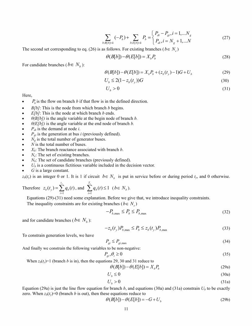
The result indicates that Line 2-3B should to be built. The optimal output of the generators and the power flow results are shown in Fig. 6.

13

1 2

3

1 4.0gP =

3 0.4gP =

2 3.4gP =

1 4.0dP =

3 3.0dP =

2 0.8dP =

0.6

0.6 1.01.0

Fig. 6: Simulation result for the transmission circuit planning

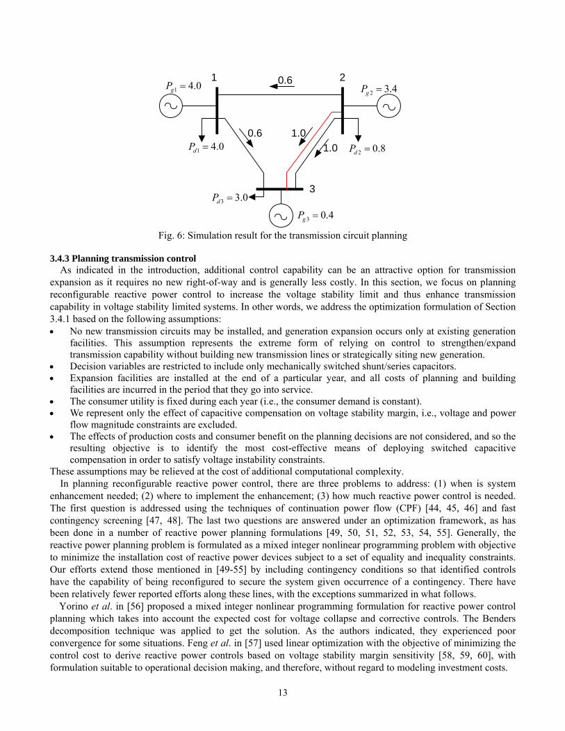
3.4.3 Planning transmission control

As indicated in the introduction, additional control capability can be an attractive option for transmission expansion as it requires no new right-of-way and is generally less costly. In this section, we focus on planning reconfigurable reactive power control to increase the voltage stability limit and thus enhance transmission capability in voltage stability limited systems. In other words, we address the optimization formulation of Section 3.4.1 based on the following assumptions: • No new transmission circuits may be installed, and generation expansion occurs only at existing generation

facilities. This assumption represents the extreme form of relying on control to strengthen/expand transmission capability without building new transmission lines or strategically siting new generation.

• Decision variables are restricted to include only mechanically switched shunt/series capacitors. • Expansion facilities are installed at the end of a particular year, and all costs of planning and building

facilities are incurred in the period that they go into service. • The consumer utility is fixed during each year (i.e., the consumer demand is constant). • We represent only the effect of capacitive compensation on voltage stability margin, i.e., voltage and power

flow magnitude constraints are excluded. • The effects of production costs and consumer benefit on the planning decisions are not considered, and so the

resulting objective is to identify the most cost-effective means of deploying switched capacitive compensation in order to satisfy voltage instability constraints.

These assumptions may be relieved at the cost of additional computational complexity. In planning reconfigurable reactive power control, there are three problems to address: (1) when is system

enhancement needed; (2) where to implement the enhancement; (3) how much reactive power control is needed. The first question is addressed using the techniques of continuation power flow (CPF) [44, 45, 46] and fast contingency screening [47, 48]. The last two questions are answered under an optimization framework, as has been done in a number of reactive power planning formulations [49, 50, 51, 52, 53, 54, 55]. Generally, the reactive power planning problem is formulated as a mixed integer nonlinear programming problem with objective to minimize the installation cost of reactive power devices subject to a set of equality and inequality constraints. Our efforts extend those mentioned in [49-55] by including contingency conditions so that identified controls have the capability of being reconfigured to secure the system given occurrence of a contingency. There have been relatively fewer reported efforts along these lines, with the exceptions summarized in what follows.

Yorino et al. in [56] proposed a mixed integer nonlinear programming formulation for reactive power control planning which takes into account the expected cost for voltage collapse and corrective controls. The Benders decomposition technique was applied to get the solution. As the authors indicated, they experienced poor convergence for some situations. Feng et al. in [57] used linear optimization with the objective of minimizing the control cost to derive reactive power controls based on voltage stability margin sensitivity [58, 59, 60], with formulation suitable to operational decision making, and therefore, without regard to modeling investment costs.

14

In the remainder of this section, a comprehensive methodology is described to address long-term reactive power control planning under the previous stated assumptions. Basic background on contingency screening and continuation power flow techniques are described in Section 3.4.3.1. Then the main steps of the proposed planning procedure, illustrated in Fig. 7, are summarized as follows. • Step 1: Identify the generation/load growth future (See Section 3.4.3.2 A). • Step 2: Assess voltage stability by fast contingency screening and the CPF techniques for each horizon year.

The year when the voltage stability margin becomes less than the required value is the time to enhance the transmission system by adding reactive power controls (See Section 3.4.3.2 B).

• Step 3: Select candidate control locations using a graph-search method (See Section 3.4.3.2 C). • Step 4: Refine location and amount of controls based on mixed integer programming and linear programming.

The optimization formulation is to minimize the total installation cost including fixed cost and variable cost of new controls while satisfying the voltage stability margin requirement under normal and contingency conditions. The branch-and-bound and primal-dual interior-point methods [ 61 ] are used to solve the optimization problem. (See Section 3.4.3.2 D.)

Develop generation/load growth future for each stage

Analyze voltage stability margin for the base case and under contingencies by fast

screening and CPF

SatisfactoryMargin?

Yes

No

Select candidate control locations using a graph-

search method

Solve the mixed integer optimization problem to find

the control location and amount

Update control location and amount

Check voltage stability margin using CPF

SatisfactoryMargin?

Solve the linear optimization problem to refine the control

amount

Update control amount

Yes

No

Step 1

Step 2

Step 3

Step 4

Fig. 7: Flowchart for the reactive power control planning 3.4.3.1 Voltage Stability Margin and Margin Sensitivity

In this section, the notion of voltage stability margin and its sensitivity to parameters are defined, for such sensitivities are used in the planning procedure. Voltage stability margin is defined as the distance between the nose point (the saddle node bifurcation point) of the system power-voltage (PV) curve and the forecasted total system real power load as shown in Fig. 8. The potential for contingencies such as unexpected component (generator, transformer, transmission line) outages often reduces the voltage stability margin [62, 63, 64]. Our objective is to find effective and economic reactive power controls to satisfy margin requirements under a set of specified contingencies. Reactive controls can be adopted to increase the voltage stability margin. Generally, series and shunt capacitors improve voltage stability margin [64]. Figure 8 shows the voltage stability margin under different operating conditions and controls.

15

Vol

tage

Real Power

M0

M2

M1

forecasted load

normal

contingency

control

M0: normal voltage stability marginM1: reduced voltage stability marginM2: increased voltage stability margin

Fig. 8: Voltage stability margin for different operating conditions

One indicator which we will find very useful in planning reactive power controls is how much control is

needed for the requirement of a given amount of margin increase. Margin sensitivities [58, 59, 60] are used to address this issue. Margin sensitivities provide the variation of the voltage stability margin with respect to any small change of power system parameter or control variable. The margin sensitivity may be used to estimate voltage stability margin if the variation of the control variable is small [59]. A typical voltage stability margin requirement is 5% under normal and “N-1” contingency conditions [65]. In addition, margin sensitivity is useful in selecting candidate control locations [56, 57]. In the following, the analytical expression of the margin sensitivity is given. The details of the margin sensitivity can be found in [58, 59, 60].

Suppose that the steady state of the power system satisfies a set of equations expressed in the vector form ( , , ) 0F x p λ = (38)

where x is the vector of state variables, p is any parameter in the power system steady state equations such as the susceptance of shunt capacitors or the reactance of series capacitors, λ is the bifurcation parameter which is a scalar. At the nose point of the system PV curve, the value of the bifurcation parameter is denoted λ*.

A specified system scenario can be parameterized by λ as 0(1 )li lpi liP K Pλ= + (39)

0(1 )li lqi liQ K Qλ= + (40) 0(1 )gj gj gjP K Pλ= + (41)

where Pli0 and Qli0 are the initial loading conditions at the base case where λ is assumed to be zero, and Qli0= Pli0tan(ψi) (where ψi is the power factor angle of the ith load). Klpi and Klqi are factors characterizing the load increase pattern. Pgj0 is the real power generation at bus j at the base case. Kgj represents the generator load pick-up factor. The voltage stability margin can be expressed as

*0 0

1 1 1

n n n

li li lpi lii i i

M P P K Pλ= = =

= − =∑ ∑ ∑ (42)

The sensitivity of the voltage stability margin with respect to the control variable at location i, Si, is *

01

n

i lpi liii i

MS K Pp p

λ=

∂ ∂= =∂ ∂ ∑ (43)

In (43), the bifurcation parameter sensitivity with respect to the control variable pi evaluated at the nose point of the system PV curve is

* **

* *ip

i

w Fp w Fλ

λ∂= −

∂ (44)

where w is the left eigenvector corresponding to the zero eigenvalue of the system Jacobian Fx, Fλ is the derivative of F with respect to the bifurcation parameter λ, and Fpi is the derivative of F with respect to control variables such as shunt capacitor susceptance or series capacitor reactance.

16

3.4.3.2 Reactive Control Planning Algorithm The proposed reactive power control planning approach requires 4 steps: (A) development of generation/load

growth future, (B) contingency selection, (C) selection of candidate control locations, and (D) refinement of locations and amounts of capacitive controls via a mixed integer programming and linear programming problems. These steps are described in the remainder of this section. It is assumed that this algorithm is applied to a power system model representing a specific future year. This is a simplifying assumption that removes from the problem the issue of when different enhancements should be implemented. A. Development of Generation and Load Growth Futures: In this step, the generation/load growth future is identified, where the future is characterized by a load growth percentage for each load bus and a generation allocation for each generation bus. For example, one future may assume uniformly increasing load at 5% per year and allocation of that load increase to existing generation (with associated increase in unit reactive capability) based on percentage of total installed capacity. Such generation/load growth future can be easily implemented in the CPF program [44] by parameterization as shown in (39), (40) and (41). B. Voltage Stability Assessment by Fast Contingency Screening: We use the CPF program to calculate the voltage stability margin of the system under each credible contingency. However, the CPF algorithm is computation-intensive. Margin sensitivities can be used to reduce computation in the screening analysis, using a standard screening approach [48]. First, the CPF program is used to calculate the voltage stability margin for the base case, and second, margin sensitivities are computed with respect to line admittances Sl and bus power injections Spq. For circuit outages, the voltage stability margin is estimated as ( ) (0)k

lM M S l= + Δ (45) where M(k) is the voltage stability margin under contingency k, M(0) is the voltage stability margin under base case conditions, and lΔ is the negative of the admittance vector for the outaged circuits. For generator outages, the voltage stability margin is estimated as ( ) (0)k

pqM M S pq= + Δ (46) where Δpq is the negative of the output power of the outaged generators. Then contingencies are ranked from most to least severe according to the value of the estimated voltage stability margin. After the ordered contingency list is obtained, we evaluate each contingency using the CPF program and stop testing after encountering N sequential contingencies that have the voltage stability margin greater than or equal to the required value, where N depends on the size of the contingency list. C. Selection of Candidate Control Locations: To select appropriate candidate reactive power control locations [56, 57] the following procedure is applied: 1) Choose an initial set of switch locations using the bisection approach for each identified contingency possessing unsatisfactory voltage stability margin according to the following 2 steps:

a) Rank the feasible control locations according to the numerical value of margin sensitivity in descending order with location 1 having the largest margin sensitivity and location n having the smallest margin sensitivity. b) Estimate the voltage stability margin with top half of the switches closed as ⎣ ⎦

∑=

+=2/

1

)()()(max

)(n

i

kki

ki

kest MSXM (47)

where )(kestM is the estimated voltage stability margin and |_n/2_| is the largest integer less than or equal to

n/2. If the estimated voltage stability margin is greater than the required value, then the number of control locations is halved, otherwise the number of control locations is increased by adding the remaining half. c) Continue in this manner until the set of control locations that satisfies the voltage stability margin requirement are identified.

2) Refine candidate control locations for each identified contingency possessing unsatisfactory voltage stability margin using the backward/forward search algorithm (described below). The final candidate control locations are the union of the locations identified for all contingencies.

The backward/forward search algorithm is described as follows. Consider a graph where each node represents a configuration of discrete switches, and two nodes are connected if and only if they are different in one switch configuration. The graph has 2n nodes where n is the number of switches. We pictorially conceive of this graph as consisting of layered groups of nodes, where each successive layer (moving from left to right) has one more

17

switch “on” (or “closed”) than the layer before it, and the tth layer (where t=0,…,n) consists of a number of nodes equal to n!/t!(n-t)!. Fig. 9 illustrates such a graph for the case of 4 switches, referred to as an automaton. The backward/forward search algorithm operates on this graph by beginning at an initial node and searching from that node in a prescribed direction, either backwards or forwards. The two extreme cases are either searching backward from the node corresponding to all switches closed (the strongest node) or searching forward from the node corresponding to all switches open (the weakest node). We give only the backward algorithm here since the forward algorithm is similar. The algorithm has 4 steps.

Pre-contingency state

(1111)

(1110)

(1011)

(1101)

(0111)

(1100)

(1010)

(0110)

(1001)

(0101)

(0001)

(0011)

(1000)

(0100)

(0010)

(0000)

Post-contingency state, no switches on

All switches on

Fig. 9: Automaton for 4-switch problem

1. Select the node corresponding to all switches in the initial set that are closed. 2. For the selected node, check if voltage stability margin requirement is satisfied for the concerned contingency

on the list. If not, then stop, the solution corresponds to the previous node (if there is a previous node, otherwise no solution exists).

3. For the selected node, eliminate (open) the switch that has the smallest margin sensitivity. We denote this as switch i*:

{ }( )* arg minc

kii

i S∈Ω

= (48)

where cΩ ={set of closed switches for the selected node}, ( )kiS is the margin sensitivity with respect to the

susceptance of shunt capacitors or the reactance of series capacitors under contingency k, at location i. 4. Choose the neighboring node corresponding to the switch i* being off. If there is more than one switch

identified in step 3, i.e. |i*|>1, then choose any one of the switches in i* to eliminate (open). Return to step 2. If step 2 of the above procedure results in no solution in the first iteration, then no previous node exists. In this case, we extend the graph in the forward direction by adding a new switch j* that has the largest margin sensitivity, expressed by

{ }( )* arg maxc

kii

j S∈Ω

= (49)

D. Refinement of Location and Amount of Capacitive Controls: This step is formulated as a mixed integer program (MIP) which minimizes control installation cost while increasing voltage stability margin to an arbitrarily specified percentage x:

Minimize

1 2

( ) ( )vi i fi i vj j fj ji j

F C B C q C X C q∈Ω ∈Ω

= + + +∑ ∑ (50)

subject to

18

1 2

( ) ( ) ( ) ( ) ( )0

k k k k ki i j j l

i jS B S X M xP

∈Ω ∈Ω

+ + ≥∑ ∑ (51)

min maxi i i i iB q B B q≤ ≤ (52)

min maxj j j j jX q X X q≤ ≤ (53) ( )0 k

i iB B≤ ≤ (54) ( )0 k

j jX X≤ ≤ (55)

, 0,1i jq = (56) Here, • Cf is fixed installation cost and Cv is variable cost of shunt or series capacitor switches, • iB is the size (susceptance) of the shunt capacitor at location i, • jX is the size (reactance) of the series capacitor at location j, • qi=1 if the location i is selected for reactive power control expansion, otherwise, qi=0, • the superscript k represents the contingency that leads the voltage stability margin to be less than the required

value, • Ω1 is the set of candidate locations to install shunt capacitor switches,

• Ω2 is the set of candidate locations to install series capacitor switches, • ( )k

iB is the size of the shunt capacitor to be switched on at location i under the contingency k, • ( )k

jX is the size of the series capacitor to be switched on at location j under the contingency k, • ( )k

iS is the sensitivity of the voltage stability margin with respect to the susceptance of the shunt capacitor at location i under contingency k,

• ( )kjS is the sensitivity of the voltage stability margin with respect to the reactance of the series capacitor at

location j under contingency k, • x is an arbitrarily specified voltage stability margin in percentage, • Pl0 is the forecasted system load, • ( )kM is the voltage stability margin under contingency k and without controls, • miniB is the minimal size of the shunt capacitor at location i, • maxiB is the maximal size of the shunt capacitor at location i, • minjX is the minimal size of the series capacitor at location j, and • maxjX is the maximal size of the series capacitor at location j.

For k contingencies that have the voltage stability margin less than the required value and n pre-selected candidate control locations, there are n•(k+2) decision variables and k+3n+2kn constraints. Fortunately, the number of candidate control locations can be limited to a relative small number even for problems of the size associated with practical power systems by assessing the combined effective index. Therefore, computational burden for solving the above MIP is not excessive even for large power systems. We solve this MIP using a branch and bound solution algorithm.

The output of the MIP is the control locations and amounts for all k contingencies and the combined control location and amount. For each contingency, the identified controls are switched in, and the voltage stability margin is recalculated to check if sufficient margin is achieved. However, because we use linear margin sensitivities to estimate the effect of the variations of control variables on the voltage stability margin, there may be contingencies that have voltage stability margin less than the required value after the network configuration is updated according to the results of the MIP. The control amount can be further refined by recomputing the margin sensitivity after the controls are updated under each contingency and adjusting the control amount via a second-stage linear program (LP) with control locations fixed at the locations found in the MIP. This LP is therefore formulated to minimize the adjusted installation cost subject to the constraint of the voltage stability

19

margin requirement, as follows: minimize

' '1 2

vi i vj ji j

F C B C X∈Ω ∈Ω

= Δ + Δ∑ ∑ (57)

subject to

' '1 2

( ) ( ) ( )( ) ( )0

k k kk ki ji j l

i j

S B S X M xP∈Ω ∈Ω

Δ + Δ + ≥∑ ∑ (58)

max0 i i iB B B≤ + Δ ≤ (59)

max0 j j jX X X≤ +Δ ≤ (60) ( ) ( )0 k ki i i iB B B B≤ + Δ ≤ +Δ (61)

( ) ( )0 k kj j j jX X X X≤ +Δ ≤ +Δ (62)

Here, • iBΔ is the adjusted size of the shunt capacitor at location i, • jXΔ is the adjusted size of the series capacitor at location j, • '

1Ω is the set of identified locations to install shunt capacitors by solving the mixed integer programming problem,

• '2Ω is the set of identified locations to install series capacitors by solving the mixed integer programming

problem, •

( )kiS is the updated sensitivity of the voltage stability margin with respect to the susceptance of the shunt

capacitor at location i under contingency k, •

( )kjS is the updated sensitivity of the voltage stability margin with respect to the reactance of the series

capacitor at location j under contingency k, • ( )k

iBΔ is the adjusted size of the shunt capacitor at location i under contingency k , • ( )k

jXΔ is the adjusted size of the series capacitor at location j under contingency k , • ( )k

M is the updated voltage stability margin under the contingency k . For k contingencies and 'n computed control locations, there are ' ( 1)n k× + decision variables and ' '2 2k n kn+ +

constraints. Again, by limiting the number of candidate control locations, computational requirements for this problem are not excessive, even for large systems. The above LP will provide good solutions because the voltage stability margin sensitivity can precisely predict the control amount under small deviation requirement of the voltage stability margin. Usually the deviation requirement of the voltage stability margin is relatively small after solving the first stage MIP. Re-solving once, beginning from the first solution, can result in small improvements, but we have not found subsequent solutions to significantly change. We solve this LP using a primal-dual interior-point method. Example 2: Optimal transmission expansion by control

The approach described in the previous section is illustrated in this section using a small 9-bus test system modified from [66] and shown in Fig. 10. The forecasted system load at the base case is 372.2 MW, and generators are economically dispatched. Table 3 shows the system loading and generation for the base case.

20

4

5 6

72

8 93

Load C

Load A Load B

1

G2 G3

G1

T2 T3

T1

Fig. 10: Modified WSCC nine-bus test system.

Table 3: Base Case System Loading and Generation

Load A

Load B

Load C

G1 G2 G3

MW 147.70 106.34 118.16 128.97 163.0 85.0 Mvar 59.08 35.45 41.36 41.39 16.72 -1.94

In the simulations, loads are modeled as constant power, voltage margin is computed assuming constant power factor at the loads, with load and generation scaled proportionally, and contingencies are assumed to be equally likely. In addition, the required voltage stability margin is assumed to be 15% for selection of candidate control locations (Step C) and 10% for refinement (Step D). The less restrictive margin requirement in location selection provides for a larger set of candidate locations that are used as input to the refinement set. Parameter values adopted in the procedure are given in Table 4.

Table 4: Parameter Values Adopted

in the Optimization Problem Shunt

capacitor Series capacitor

Variable cost Cvi=0.15 Cvj=0.35 Fixed cost Cfi=0.13 Cfj=0.25 Maximum size Bimax=0.16 Xjmax=0.03 Minimum size Bimin=0.001 Xjmin=0.001

For each bus, consider the simultaneous outage of 2 components (generators, lines, transformers) connected to

the bus. There exist 2 contingencies that reduce the post-contingency voltage stability margin to less than 10% as shown in Table 5.

Table 5: Voltage Stability Margin for Severe Contingencies Contingency Voltage Stability Margin (%) 1. Outage of lines 5-4A and 5-4B 4.73 2. Outage of transformer T1 & line 4-6 4.67

We first plan candidate locations of shunt capacitors under the outage of lines 5-4A and 5-4B. Table IV

summarizes the steps taken by the backward search algorithm in terms of switch sensitivities, where we have assumed the susceptance of shunt capacitors to be installed at feasible buses ( )

max 0.16 . .ki i iB B B p u= = = The initial

network configuration has six shunt capacitors at buses 4, 5, 6, 7, 8, and 9 are switched on. The voltage stability margin with all six shunt capacitors switched on is 11.34% which is greater than the required value of 10%.

21

Therefore, the number of switches can be decreased to reduce the cost. At the first step of the backward search, we compute the margin sensitivity for all six controls as listed in the 4th column. From this column, we see that the row corresponding to the shunt capacitor at bus 4 has the minimal sensitivity. So in this step of backward search, this capacitor is excluded from the list of control locations indicated by the strikethrough. Continuing in this manner, in the next three steps of the backward search we exclude shunt capacitors at buses 6, 9, and 8 sequentially. However as seen from the last column of Table 6, with only 2 controls at buses 5 and 7, the voltage stability margin is unacceptable at 9.51%. Therefore the final solution must also include the capacitor excluded at the last step, i.e., the shunt capacitor at bus 8. The location of these controls are intuitively pleasing given that, under the contingency, Load A, the largest load, must be fed radially by a long transmission line, a typical voltage stability problem.

Table 6: Steps Taken in the Backward Search Algorithm for Shunt Capacitor Planning

No no cntrl. 6 cntrls.5 cntrls. (reject #6)

4 cntrls. (reject#5)

3 cntrls. (reject#4)

2 cntrls. (reject#3)

1 Sens. of shunt cap. at bus 5 0.738 0.809 0.808 0.807 0.804 0.756 2 Sens. of shunt cap. at bus 7 0.334 0.360 0.359 0.358 0.357 0.352 3 Sens. of shunt cap. at bus 8 0.240 0.263 0.262 0.261 0.260 4 Sens. of shunt cap. at bus 9 0.089 0.098 0.097 0.096 5 Sens. of shunt cap. at bus 6 0.046 0.051 0.051 6 Sens. of shunt cap. at bus 4 0.019 0.021 loadability (MW) 389.8 414.4 414.0 413.2 411.7 407.6 loading margin (%) 4.73 11.34 11.24 11.02 10.61 9.51

Reject the shunt capacitor at bus 4

Reject the shunt capacitor at bus 6

Reject the shunt capacitor at bus 9

R O

Fig. 11: Graph for the backward search algorithm for shunt capacitor planning.

Fig. 11 shows the corresponding search via the graph. In the figure, node O represents the origin configuration

of discrete switches from where the backward search originates, and node R represents the restore configuration associated with a minimal set of discrete switches which satisfies the voltage stability margin requirement (this is the node where the search ends).

For the outage of transformer T1 and line 4-6, the solution obtained by the forward search algorithm is: shunt capacitors at buses 4 and 5. Therefore, the final candidate locations for shunt capacitors are buses 4, 5, 7, and 8 which guarantee that the voltage stability margin under all prescribed N-2 contingencies is greater than the required value. In a similar way, we obtain the final candidate locations for series capacitors as lines 5-7A and 5-7B where we have assumed the reactance of series capacitor to be installed in feasible lines ( )

max 0.03 . .ki i iX X X p u= = = . Therefore, the best six candidate locations are lines 5-7A, 5-7B to install series

22

capacitor switches, buses 4, 5, 7, 8 to install shunt capacitor switches. We use these candidate locations to initialize the reactive power planning algorithm presented in Section III was carried out.

In order to demonstrate the efficacy of the proposed method, two cases are considered as follows. In case one, only shunt capacitor switches are chosen as candidate controls while both shunt and series capacitor switches are chosen as candidate controls in case two. Table 7 shows the results for case one where the optimal allocations for shunt capacitor switches are 0.16, 0.16, and 0.115 pu at buses 5, 7, and 8, respectively, and these switches are fully used for the outage of transformer T1 and line 4-6. The total cost is 0.451 for the control allocations in case 1. On the other hand, the optimal control allocations for case two are shown in Table 8 indicating that a series capacitor switch of 0.03 pu on line 5-7A and a shunt capacitor switch of 0.131 at bus 5, and these switches are fully used for the outage of transformer T1 and line 4-6. For case two, the total cost for control allocations is 0.41 which is 9.96% less than that of case one. This result shows that benefit can be obtained by pursuing a strategy of planning different types of discrete reactive power controls. Table 9 gives the verified results of the reactive power control planning with the continuation power flow program. The voltage stability margins of the concerned contingencies are approximately equal to the required value of 10% under the planned controls. The iteration number in the second column represents the number of times of solving the LP after solving the MIP.

Table 7: Control Allocations with Shunt Capacitors Candidate

locations for shunt capacitors

Maximum size

Result for the whole problem

Result for

cont. 1

Result for

cont. 2Bus 5 0.16 0.16 0.156 0.16 Bus 4 0.16 0.00 0.00 0.00 Bus 7 0.16 0.16 0.16 0.16 Bus 8 0.16 0.088 0.082 0.088

Table 8: Control Allocations with Shunt and Series Capacitors

Candidate locations for

shunt and series caps

Maximum size for

shunt caps

Result for the whole problem

Result for

cont. 1

Result for

cont. 2

Line 5-7A 0.03 0.03 0.03 0.03 Line 5-7B 0.03 0.00 0.00 0.00

Bus 5 0.16 0.131 0.105 0.131Bus 4 0.16 0.00 0.00 0.00 Bus 7 0.16 0.00 0.00 0.00 Bus 8 0.16 0.00 0.00 0.00

Table 9: Voltage Stability Margin under Planned Controls

Candidate control

Iteration number for

LP

Voltage stability

margin for cont. 1

Voltage stability

margin for cont. 2

Shunt caps 1 9.98% 10.01% Shunt and series caps

1

10.01% 9.99%

This section has presented an optimization-based approach for planning reactive power control in electric power transmission systems to satisfy voltage stability margin requirements under normal and contingency conditions. The planned reactive power controls are capable of serving as control response for contingencies. Optimal locations and amounts of new switch controls are obtained by solving the MIP. The amount of control is further refined by solving the LP. The proposed algorithm can handle a large-scale power system because it

23

significantly reduces computation burden by fully utilizing the information of the voltage stability margin sensitivity and overcomes the possible difficulty of convergence associated with nonlinear programming formulations. The effectiveness of the method is illustrated by using a test system. The results show that the method works satisfactorily to plan reactive power control. 3.4.4 Dynamic analysis

In Section 3.4.3, we described procedures for planning control to expand transmission at minimum cost under constraints imposed by post-transient reliability criteria. These procedures resulted in optimal locations and amounts of shunt and series capacitors, but because analysis was based on purely static models, constraints associated with transient reliability criteria were not enforced. Although the resulting solutions provide very useful guides in regards to the investments necessary to appropriately expand transmission, there remain unanswered questions about control design, in particular, given the availability of the switchable shunt and series capacitors as determined from the static analysis, for each contingency: What sequence of switches and associated timing is necessary in order to satisfy the transient reliability criteria? Table 1 indicates two types of transient reliability criteria: one is on voltage deviations and the other is on frequency deviations. An implied necessary condition is that the system be stable.

The problem of designing the control for a specified contingency has three steps, as follows: 1. Identify the switches (each leading to series or shunt capacitor insertion) to be operated. 2. Identify the sequence of switch operations. 3. Determine the timing of each switch operation. We assume that the solution for step 1 is obtained from the static analysis described in Section 3.4.3. This assumption may not always be valid, i.e., the controls that result in acceptable post-transient conditions do not necessarily provide for acceptable transient conditions independent of their sequence or timing, and in such a case, one may need to augment the switches identified in Step 13. For step 2, there are n! possible solutions, where n is the number of switches identified in step 1. Each possible solution corresponds to a path through the automaton; for example, in the 4-switch case of Fig. 9, there are 4!=24 paths or switching sequences. There may be a number of acceptable sequences, depending on the range of switching times as determined in Step 3.

A commonly used method for the dynamic performance analysis of a control is time domain simulation. For each initial fault-on state, one performs simulation for each control in order to find an effective one. For the planning problem, when there are multiple operating conditions, multiple contingencies, and multiple control possibilities, this is ad-hoc and labor-intensive method. Alternatively, methods based on determination of stability regions may be more efficient for control design, particularly when discrete control strategies are considered. We approach the problem by identifying the stability region of post-fault stable equilibria associated with different switching configurations. For a general nonlinear autonomous system, the stability region is defined as the set of all points from which the trajectories start and eventually converge to the stable equilibrium point (SEP) as time approaches infinity [67].

To motivate the potential for using stability regions to address the dynamic performance analysis, consider a one machine-infinite bus system equipped with shunt and series controls as shown in Fig. 12.

δ∠E

0∠U1jX 2jX seriesjX

shuntjX

Fig. 12: System model with shunt and series control strategies

3 One efficient way to gain insight into the effectiveness of a group of switched capacitive compensators on transient performance for a transient is to simulate the transient under the conditions that all capacitors are switched at the earliest conceivable moment (simultaneous with fault clearing), and if transient criteria are not satisfied, then the group should be either be augmented, or faster controls should be employed such as static var compensators (SVCs) or thyristor-controlled-series-capacitors (TCSC).

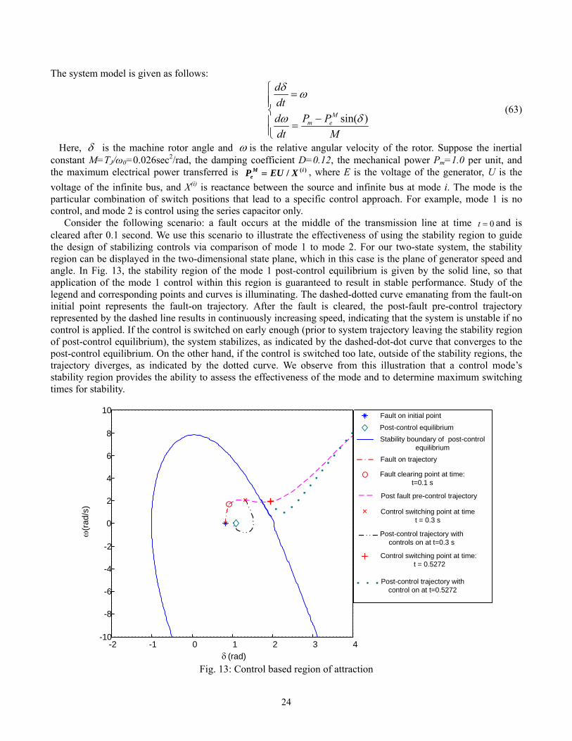
24

The system model is given as follows:

⎪⎪⎩

⎪⎪⎨

⎧

−=

=

MPP

dtddtd

Mem )sin(δω

ωδ

(63)

Here, δ is the machine rotor angle and ω is the relative angular velocity of the rotor. Suppose the inertial constant M=TJ/ω0=0.026sec2/rad, the damping coefficient D=0.12, the mechanical power Pm=1.0 per unit, and the maximum electrical power transferred is )(/ iM

e XEUP = , where E is the voltage of the generator, U is the voltage of the infinite bus, and X(i) is reactance between the source and infinite bus at mode i. The mode is the particular combination of switch positions that lead to a specific control approach. For example, mode 1 is no control, and mode 2 is control using the series capacitor only.

Consider the following scenario: a fault occurs at the middle of the transmission line at time 0=t and is cleared after 0.1 second. We use this scenario to illustrate the effectiveness of using the stability region to guide the design of stabilizing controls via comparison of mode 1 to mode 2. For our two-state system, the stability region can be displayed in the two-dimensional state plane, which in this case is the plane of generator speed and angle. In Fig. 13, the stability region of the mode 1 post-control equilibrium is given by the solid line, so that application of the mode 1 control within this region is guaranteed to result in stable performance. Study of the legend and corresponding points and curves is illuminating. The dashed-dotted curve emanating from the fault-on initial point represents the fault-on trajectory. After the fault is cleared, the post-fault pre-control trajectory represented by the dashed line results in continuously increasing speed, indicating that the system is unstable if no control is applied. If the control is switched on early enough (prior to system trajectory leaving the stability region of post-control equilibrium), the system stabilizes, as indicated by the dashed-dot-dot curve that converges to the post-control equilibrium. On the other hand, if the control is switched too late, outside of the stability regions, the trajectory diverges, as indicated by the dotted curve. We observe from this illustration that a control mode’s stability region provides the ability to assess the effectiveness of the mode and to determine maximum switching times for stability.

δ (rad)

ω(ra

d/s)

-2 -1 0 1 2 3 4-10

-8

-6

-4

-2

0

2

4

6

8

10

Stability boundary of post-control equilibrium

Fault on initial point

Post-control equilibrium

Fault on trajectory

Post fault pre-control trajectory

Post-control trajectory with controls on at t=0.3 s

Fault clearing point at time: t=0.1 s

Control switching point at time t = 0.3 s

Control switching point at time: t = 0.5272

Post-control trajectory with control on at t=0.5272

Fig. 13: Control based region of attraction

25

In the last three decades numerous efforts have been undertaken to determine the stability region with the goal of power system transient stability analysis. The studies [68, 69, 70, 71] provided the theoretical foundations for the geometric structure of the stability region. Reference [70] proved that the stability boundary of a stable equilibrium point (SEP) is the union of the stable manifolds of the type one unstable equilibrium points. It also proposed a numerical algorithm to determine the stability region. This method however is not always applicable, and even when it is applicable, the computation of stable manifold of a type one unstable equilibrium point is not easy for a large system, and even when the computation is feasible, the method can only provide local approximation of the stable manifold. Recently, some algorithms have been developed to approximate the stable manifold of an unstable equilibrium point (UEP). For example, in [72, 73] the Taylor expansion is used to obtain a quadratic approximation, whereas in [74, 75] the stable manifolds around an UEP are approximated by the normal form technique and the energy function methods [76]. A well-known alternative method called the closest unstable equilibrium point method [77] finds a subset of the true stability region and thereby need not obtain the stable manifold of an UEP. It is shown in [78] that the stability region estimated by the closest UEP method is optimal in the sense that it is the largest region within the stability region, which can be characterized by the corresponding energy function. These energy function/Lyapunov based methods however can only provide a conservative estimate of a stability region. Furthermore, these methods can not compute a stability region for a hybrid system.

Our method for computing the stability region of an SEP of a power system is based on backward reachability analysis as reported in [79]. Reachability analysis focuses on finding reachable sets of a target set. Reachable sets are a way of capturing the behavior of entire groups of trajectories at once. The backwards reachable set is the set of states which give rise to trajectories leading to the target set. Given a post-fault stable operating point (an SEP), there must exist an open neighborhood of it that is contained in its stability region. This means that if we choose a sufficiently small ball of radius ε around the SEP as the target set, any trajectory entering that target set is guaranteed to converge to the associated SEP. Thus, as time goes to infinity, the backward reachable set of the target set approaches the stability region of the system.

One way of describing a subset of states is via an implicit surface function representation as shown in Fig.14. Consider a closed set nRS ⊆ . An implicit surface representation of S would define a function RRx n →:)(φ such that

0)( ≤xφ if Sx∈ and 0)( >xφ if Sx∉ .

0)( >xφ

0)( =xφ 0)( <xφ

Fig. 14: Implicit surface function representation

In [80], the author formulates the backward reachable set in terms of a Hamilton-Jacobi-Isaacs (HJI) Partial

Differential Equation (PDE) and proves that the viscosity solution of this PDE is an implicit surface representation of the backward reachable set. This HJI PDE can be solved with the very accurate numerical methods drawn from the level set literature. In [81] we applied the stability region computation to determine the minimal amount of load shedding in voltage stability control.

The following algorithm summarizes the procedure to determine the stability region of a post-fault power system.

26

(1) Form the state space equations of the post-fault power system, )(xfdtdx

=

(2) Find the stable equilibrium point of this autonomous nonlinear system, by solving 0)( =xf and let nRx ∈* be a SEP.

(3) Specify aε ball centered at the stable equilibrium point with sufficiently small radiusε . (4) Define an implicit surface function at 0=t as

εφ −−= *)0,( xxx (64)

Then the target set is the zero sublevel set of the function )0,(xφ , i.e, it is given by { })0)0,(| ≤∈ xRx n φ (65)

Therefore, a point x is inside the target set if )0,(xφ is negative, outside the target set if )0,(xφ is positive, and on the boundary of the target set if )0,(xφ .

(5) Propagate in time the boundary of the backward reachable set of the target set by solving the following

HJI PDE: 0),( =+ t

Tx txf φφ (66)

with terminal conditions (64). The zero sublevel set of the viscosity solution ),( txφ to (64), (66) is the backward reachable set at time t is

{ })0),(| ≤∈ txRx n φ (67) (6) The backward reachable set of the ε ball around the stable equilibrium point is computed using a

software tool from [60]. It is always possible to find a certain epsilon-ball contained in the stability region of a stable equilibrium point. As t goes to infinity, the backward reachable set approaches the true stability region. If the stability region is bounded, the level set based numerical computation of the backward reachable set eventually converges to the stability region within a finite computation time.

We present an example to illustrate stability region computation and its application in dynamic analysis of a control strategy.

Example 3: Stability region identification for single-machine-infinite-bus Consider the system in Fig.12. Define the system with no controls on as mode 1, with series control on as mode 2, with shunt control on as mode 3, and with both series control and shunt control on as mode 4. As the mode is changed, the transmission line reactance changes causing the M

eP as well as the equilibrium point to change. Each of the 4 modes (corresponding to 2 different binary controls), the associated transmission line reactance, the

MeP value, and the equilibrium point are summarized in Table 10.

Table 10: Four control modes and their certain parameters Mode Series Capacitor Shunt Capacitor )( iX M

eP value Equilibrium points

1 Off Off 21 XX + 1.35 (0.8342, 0)

2 On Off seriesXXX −+ 21

2.25 (0.4603, 0)

3 Off On shuntXXXXX 21

21 −+ 1.543 (0.7084, 0)

4 On On

shunt

series

series

XXXXXXX

)()(

21

21

−−

−+

2.3478 (0.4400, 0)

The stability regions of all the four modes are shown in Fig. 15. The stability region of mode 1 is inside the dotted curve, that of mode 2 is inside the dashed-dot curve, that of mode 3 is inside the dashed curve, and that of mode 4

27

is inside the solid curve.

-5 0 5-20

-15

-10

-5

0

10

15

20

)(radδ

5

Mode 1

Mode 2

Mode 3

Mode 4

0

10

Fig. 15: Stability region of the 4 modes

Using the stability regions, we can verify the effectiveness of different control strategies and also provide an

effective control strategy for a given post-fault initial state. When the post-fault state is inside the stability region of mode 1, no control is needed because the state will eventually reach the stable equilibrium point. When the post-fault state is outside the stability region of mode 1, some control needs to be switched-on to stabilize the post-fault state. For example, if the initial post-fault state is inside the stability region of mode 2 and outside the stability region of mode 3, we have two choices to stabilize the system: Switch on the series capacitor or switch on both the series and shunt capacitors. The system will then converge to the stable equilibrium point of mode 2 or mode 4 accordingly. In general, if the post-fault initial state is inside the union of stability regions of all such modes, the transient stability can be achieved by switching one or more controls on. We identified the importance of dynamic analysis besides the static analysis. A dynamic analysis is needed to determine the domain over which a control strategy computed using a static analysis is effective. Stability region forms the basis of a dynamic analysis, and we presented an example to illustrate how stability region associated with various control modes can be used in devising a contingency control strategy. Our method uses backward reachability analysis involving propagation of level-sets for computing a stability region. A limitation of our method is that the computation complexity grows exponentially in the number of system dimension. This is because a computation of the backward reachable set is based on gridding of the state space. As part of future research we plan to explore faster and/or approximate techniques for reachability computation. This includes possibility of parallelization, of hierarchical computation, and Sum of Squares (SOS) based approach. 3.5 MARKET EFFICIENCY AND TRANSMISSION INVESTMENT As competitive reforms are introduced into the electricity power industry, much attention has been focused on the potential market organization of the industry’s transmission sector. Questions have naturally risen: Shall deregulation and competition be applied to transmission, as they are to generation and distribution? To what degree shall market play a role in transmission expansion and investment?

There is some literature on transmission and transmission investment. Hogan (1992) [82] proposes a contract network pricing model, using congestion payments as the rental fee for use of the capacity rights. Within this contract network regime, Bushnell and Stoft (1996) [83] analyze the incentives for grid investment. They show that under certain conditions this contract network approach can effectively deter detrimental investments, some of which are encouraged under other regimes. Chao and Peck (1996) [84] define a trading rule and property rights so that a competitive market could be established for transmission services to achieve a social optimum within a

28

power pool. In Bushnell and Stoft (1997) [85], a process is outlined by which transmission planning and investment would be undertaken by competitive entities in a lightly regulated environment. More recently, Joskow and Tirole (2005) [86] examine the performance attributes of a merchant transmission investment framework that relies on “market driven” investment to increase transmission network capacity and conclude that inefficiencies may result from reliance on such a framework. In what follows, we will show our work that addresses something not explicitly identified in this literature.

It is well known that generation of power can be efficiently decentralized by means of a price system and competitive markets. Indeed, Chao and Peck (1996) [84] showed that for a given grid, the competitive equilibrium is efficient. That is, the competitive equilibrium nodal and transmission prices induce an efficient dispatch. It is also known that this result breaks down as soon as the grid itself is endogenous. The main example of this inefficiency is based on the fact that adding or removing a line has a dramatic change in the flow of power for any given set of injections. In the economist's jargon, there is a market failure in the power market once investment in transmission is allowed. The alleged reason for this market failure is the externalities created by loop flows4. That loop flows are responsible for the market failure is clear, since a power market with endogenous investment in a radial network can be efficiently decentralized by a market mechanism. However, the nature of the externalities created by loop-flows has, to the best of our knowledge, never been identified. Is the addition or removal of circuits necessary for markets to fail? In other words, if we only allow investment that results in an upgrade of the line capacities of a given grid, can a competitive equilibrium allocation fail to be efficient? Are the externalities created by loop flows due to the fact that changes in the line capacities affect the set of feasible injections into the grid? Are the loop-flow induced externalities related to the fact that the allowable injections in one bus depend on the injections in the other buses?

In this section we clarify the nature of the externalities introduced by the loop flows. The bottom line is that transmission investment introduces an externality only if it affects the flow of power along the lines for any given set of injections. For instance, the addition or removal of a new circuit will affect the flow of power for any given set of injections, unless of course we are adding or removing part of a radial network. But the increase of the operational capacity of a line will not introduce an externality, even if it does change the set of feasible injections, unless it affects the flow of power for any given set of injections.

As a result, we can answer the above questions as follows. The addition or removal of lines are not necessary for markets to fail: the competitive equilibrium will not be efficient even if the grid topology is restricted to remain the same but upgrades of line capacities that change the power flow are allowed. The change in the set of feasible injections itself is not responsible for the market failure: as long as the line capacities are changed in a flow-preserving way, there will be no externalities associated with the investment. Finally, the fact that injections in one bus affect the set of allowable injections in other buses is not the source of externalities. The truth of the last two statements can be seen by observing a two-bus network: in such a network, the flow structure is always the same; namely, each MW injected in one bus transits the only line, independently of its capacity.

In this section we present two examples. The first one shows that unless it leaves the flow of power for any given set of injections unaffected, transmission investment will induce externalities that cause the market to fail. The second example considers a type of investment, which consists of enhancing the operational capacity of a line by adding a capacitor that will be switched on only in case a contingency occurs. Since under normal circumstances the impedances are constant, whether the capacitor is installed or not, this type of capacity enhancement will not affect the flow structure of the network and as a result the competitive allocation will be efficient. Example 4: Transmission-induced capacity enhancement

Consider Fig. 16, where there are 3 interconnected buses, buses 1, 2 and 3 (n = 1, 2, 3). Let lines 1, 2 and 3 denote the lines connecting buses 2 and 3, buses 1 and 3 and buses 1 and 2, respectively. Originally, each line has some capacities. The capacities of line 1 and line 2 are so large, that they are never congested. Let k0 denote the initial capacity on line 3. To make things interesting, suppose k0 is less than the socially efficient capacity.

A generator is attached to buses 1 and 2, respectively, denoted by G1 and G2. G1's cost function is C1(Pg1) and G2's cost function is C2(Pg2), where, for n=1,2, Pgn is the amount of power generated and Cn is a strictly convex

4 There are externalities when the actions of one agent directly affect the payoff of the other agents associated with a given action.

29

function that satisfies Cn(0) = 0. The only load, of a constant 1000 MW, is located at bus 3. There is an investment firm that produces transmission capacity. It only chooses to build lines between buses 1 and 2, since the other two lines already have enough capacity. The investment firm's cost function is C(I), which is assumed to be strictly convex, and where I is the capacity of the new line it builds between buses 1 and 2.

1 2

3Load=1000 MW

Line 3

Line 1Line 2

G2G1

Fig 16: 3-bus example

A dispatch is a pair of injections (Pg1, Pg2) that satisfy the load, i.e. Pg1 + Pg2 = 1000. Not all dispatches are feasible. In order for a dispatch to be feasible, the flow along each line should not exceed the line's capacity. In this example, since we assume that lines 1 and 2 have large enough capacity, we are only concerned with the flow along line 3, from bus 1 towards bus 2. Clearly, the flow of power along this line depends on the dispatch. But it may also depend on the capacity of the line. For the purpose of the analysis we will adopt a linear approximation and assume that the flow of power from bus 1 to bus 2 is given by P12 = α(k)(Pg1-Pg2), where k = k0 + I is the capacity of line 3, after an investment I has been made. As we will see, the dependence of the coefficient α on the capacity of the line is the source of the market failure in the transmission investment market.

With this formulation in hand, we can define a feasible allocation to consist of a dispatch (Pg1, Pg2) and a capacity investment I, such that – (k0 + I) ≤ α(k0 + I) (Pg1 – Pg2) ≤ (k0 + I). With this notation, we are ready to solve for the optimal allocation. The optimal allocation is the transmission investment I and the dispatch (Pg1, Pg2) that satisfies the load in the least expensive way. Formally, it is the solution to the following "social planner's" problem

( )

( ) ( )( ) ( )⎪⎪⎭

⎪⎪⎬

⎫

+≤−+≤+−

=+

++

IkPPIkIk

PP

ICPCPC

gg

gg

ggIPP gg

02100

21

2211,,

1000 s.t.

)()(min21

α

(68)

For the sake of the analysis, assume that α(⋅) is such that the set of feasible allocations is convex. Also, for simplicity assume that the above problem has an interior solution and, without loss of generality, that at that solution α(k0 + I) (Pg1 – Pg2) ≥0.5 Let λ and μ be the Lagrangian multipliers of the above constraints, respectively. Then the first order conditions for an interior solution are:

( )

( )

( ) ( )( )

( )( ) ∗∗∗∗

∗∗

∗∗∗∗

∗∗

∗∗

+=−+

=+

−∂+∂

−=∂

∂

++=∂

∂

+−=∂

∂

IkPPIk

PP

PPk

IkIIC

IkP

PC

IkP

PC

gg

gg

gg

g

g

g

g

0210

21

210

02

22

01

11

1000

)(

)(

α

αμμ

μαλ

μαλ

(69)

5Sufficient conditions for an interior solution would be that marginal costs of generation and investments are 0 when evaluated at 0.

30

It follows that at an interior efficient allocation ( ) 0,>>∗∗∗ IPP gg ,, 21 ( )

( ) ( )( ) ( )∗∗∗

∂+∂

∂∂∗∗

+−−

=∂

∂−

∂∂

∗

∗

IkPPP

PCP

PC

ggkIk

IIC

g

g

g

g0

211

11

2

22

012

)()(α

α (70)

We now want to compare the efficient allocation with the outcome of decentralized trade through a price mechanism. For this we need to define the competitive equilibrium. In the following definition of economic equilibrium, there will be electricity prices associated to each bus (the nodal prices), and one transmission charge. The concept of nodal prices, is central in power system economics, and was introduced by Schweppe et al [19].

A competitive equilibrium consists of an allocation ( )( )∗∗∗ IPP gg ,, 21 and a price vector (π1,π2,π3,τ) that satisfy the following conditions. a. The transmission investing firm maximizes its profits, given the transmission price on the newly built line: it

chooses I* so as to solve ( )ICI

I−τmax (71a)

b. Each generator maximizes its profit, given its respective nodal prices: More specifically, given the nodal prices πn, n = 1,2, generator Gn, for n = 1,2, solves:

)(max gnngnnPPCP

gn

−π (71b)

c. Markets clear 1000*

2*1 =+ gg PP (71c-1)

( )( ) ∗∗∗∗ +=−+ IkPPIk gg 0210α (71c-2) d. No arbitrage opportunity exists. ( )ταππ ∗++= Ik013 (71d-1)

( )ταππ ∗+−= Ik023 (71d-2)

Conditions (71a) and (71b) can be replaced by the corresponding necessary and sufficient conditions for profit maximization as follows:

( )

τ=∂

∂ ∗

IIC

(71a')

11

11 )(π=

∂∂ ∗

g

g

PPC

(71b'-1)

22

22 )(π=

∂∂ ∗

g

g

PPC

(71b'-2)

Suppose that an allocation ( )( )∗∗∗ IPP gg ,, 21 and a price vector (π1,π2,π3,τ) constitute a competitive equilibrium. Then, from the no-arbitrage conditions we have

( )( )ταππ

ταππ∗

∗

+−=

++=

Ik

Ik

023

013 (72)

Substituting into the generators' first order conditions (71b'-1) and (71b'-2), we get

( )

( )ταπ

ταπ

∗∗

∗∗

+−∂

∂=

++∂

∂=

IkP

PC

IkP

PC

g

g

g

g

02

223

01

113

)(

)(

(73)

Replacing the transmission prices with the marginal costs, from equation (71a') and rearranging it, we get

31

( )IIC

PPC

PPC

g

g

g

g

∂∂

=∂

∂−

∂∂ ∗∗∗

2)()(

1

11

2

22 ( )∗kα (74)

Comparing equations (70) and (74), we see that unless ( ) 00 =∂+∂ ∗

kIkα , that is, unless investment does not affect the

power distribution factor α, we cannot guarantee that the competitive equilibrium be efficient. This allows us to conclude that the source of the market failure lies on the fact that investment in transmission capacity affects the power flow through the lines for any given dispatch.

Can, nevertheless, some government intervention achieve an efficient allocation via a decentralized market mechanism? The answer is yes, if we have enough information to apply the optimal Pigouvian tax. Suppose that the government imposes an ad-valorem tax t on capacity enhancement. Then the investment firm's profit maximization problem becomes ( )ICIt

I−− )1(maxτ (75)

The profit maximizing investment satisfies the first order condition

( ) )1( tIIC

−=∂

∂ ∗

τ (76)

and the conditions that a competitive equilibrium satisfies are

( )

22

22

11

11

)(

)(

)1(

π

π

τ

=∂

∂

=∂

∂

−=∂

∂

∗

∗

∗

g

g

g

g

PPC

PPC

tIIC

(77)

( )( )

( )( )ταππ

ταππ

α

∗

∗

∗∗∗∗

∗∗

−=

+=

=−

=+

k

k

kPPk

PP

gg

gg

23

13

21

21 1000

By comparison, we can see that if allocation ( )( )∗∗∗ IPP gg ,, 21 solves the social optimum problem (68) with

associated Lagrangian multipliers (λ, μ), then the same allocation ( )( )∗∗∗ IPP gg ,, 21 together with the price vector

( )∗∗∗∗ τπππ ,,, 321 and ad-valorem tax rate t* defined by

( )( )

( )( )∗∗∗

∗

∗

∗∗

∗∗

−∂+∂

=

=

=

+=

−=

210*

3

2

1

gg

g

g

PPk

Ikt

kP

kP

α

μτ

λπ

μαλ

μαλ

(78)

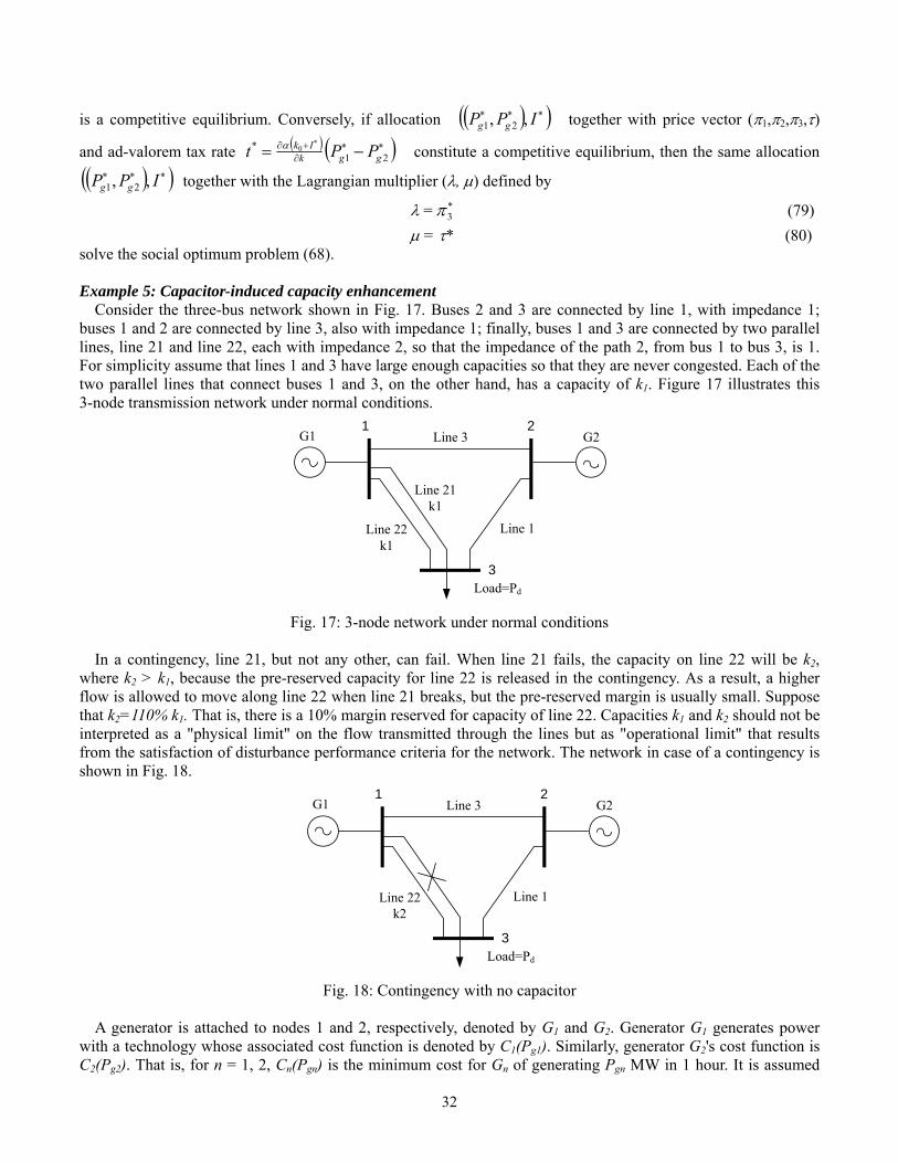
32

is a competitive equilibrium. Conversely, if allocation ( )( )∗∗∗ IPP gg ,, 21 together with price vector (π1,π2,π3,τ)

and ad-valorem tax rate ( ) ( )∗∗∂+∂ −=

∗

21* 0

ggkIk PPt α constitute a competitive equilibrium, then the same allocation

( )( )∗∗∗ IPP gg ,, 21 together with the Lagrangian multiplier (λ, μ) defined by

λ = ∗3π (79)

μ = τ* (80) solve the social optimum problem (68). Example 5: Capacitor-induced capacity enhancement

Consider the three-bus network shown in Fig. 17. Buses 2 and 3 are connected by line 1, with impedance 1; buses 1 and 2 are connected by line 3, also with impedance 1; finally, buses 1 and 3 are connected by two parallel lines, line 21 and line 22, each with impedance 2, so that the impedance of the path 2, from bus 1 to bus 3, is 1. For simplicity assume that lines 1 and 3 have large enough capacities so that they are never congested. Each of the two parallel lines that connect buses 1 and 3, on the other hand, has a capacity of k1. Figure 17 illustrates this 3-node transmission network under normal conditions.

1 2

3Load=Pd

Line 3

Line 1Line 22k1

G2G1

Line 21k1

Fig. 17: 3-node network under normal conditions

In a contingency, line 21, but not any other, can fail. When line 21 fails, the capacity on line 22 will be k2,

where k2 > k1, because the pre-reserved capacity for line 22 is released in the contingency. As a result, a higher flow is allowed to move along line 22 when line 21 breaks, but the pre-reserved margin is usually small. Suppose that k2=110% k1. That is, there is a 10% margin reserved for capacity of line 22. Capacities k1 and k2 should not be interpreted as a "physical limit" on the flow transmitted through the lines but as "operational limit" that results from the satisfaction of disturbance performance criteria for the network. The network in case of a contingency is shown in Fig. 18.

1 2

3Load=Pd

Line 3

Line 1Line 22k2

G2G1

Fig. 18: Contingency with no capacitor

A generator is attached to nodes 1 and 2, respectively, denoted by G1 and G2. Generator G1 generates power

with a technology whose associated cost function is denoted by C1(Pg1). Similarly, generator G2's cost function is C2(Pg2). That is, for n = 1, 2, Cn(Pgn) is the minimum cost for Gn of generating Pgn MW in 1 hour. It is assumed

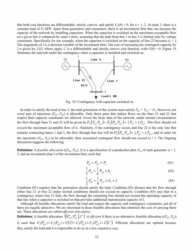
33

that both cost functions are differentiable, strictly convex, and satisfy Cn(0) = 0, for n = 1, 2. At node 3, there is a constant load of Pd MW. Apart from generators and consumers, there is an investment firm that can increase the capacity of the network by installing capacitors. When the capacitor is switched on the maximum acceptable flow on a given line is enhanced by some I units, assuming that the path from bus 1 to bus 3 is limited only by voltage constraints. Specifically for our example, when the capacitor is switched on the capacity of line 22 becomes k2 + I. The magnitude of I is a decision variable of the investment firm. The cost of increasing the contingent capacity by I is given by, C(I), where again, C is a differentiable and strictly convex cost function, with C(0) = 0. Figure 19 illustrates the network under the contingency when a capacitor is installed and switched on.

Fig. 19: Contingency with capacitor switched on

In order to satisfy the load in bus 3, the total generation of the system must satisfy Pg1 + Pg2 = Pd. However, not

every pair of injections (Pg1, Pg2) is allowable. Only those pairs that induce flows on the lines 21 and 22 that respect their capacity constraints are allowed. Given the basic data of the network, under normal circumstances the flow through lines 21 and 22 will be given by ( ) ( )== 2,1222,121 gggg PPPPPP 26

113

1gg PP + . This flow should not

exceed the maximum acceptable flow of k1. Similarly, if the contingency occurs and line 22 is the only line that remains connecting buses 1 and 3, the flow through that line will be ( )=2,122 gg

c PPP 241

121

gg PP + , and in order for the injections (Pg1, Pg2) to be allowable, their associated contingent flow should not exceed k2 + I. The forgoing discussion suggests the following.

Definition: A feasible allocation ((Pg1, Pg2), I) is a specification of a production plan Pgn of each generator n = 1, 2, and an investment plan I of the investment firm, such that dgg PPP =+ 21 (81)

121 61

31 kPP gg ≤+ (82)

.41

21

221 IkPP gg +≤+ (83)

Condition (81) requires that the generation should satisfy the load. Condition (82) dictates that the flow through either line 21 or line 22 under normal conditions should not exceed its capacity. Condition (83) says that in a contingency where line 21 fails, the flow through the remaining line should not exceed the operating capacity of that line when a capacitor is switched on that provides additional transmission capacity of I.

Although all feasible allocations satisfy the load and respect the capacity and contingency constraints, not all of them are equally attractive. We are interested in those feasible allocations that minimize the cost of carrying them out. These allocations are called efficient allocations. Definition: A feasible allocation ( )( )∗∗∗ IPP gg ,, 21 is efficient if there is no alternative feasible allocation ((Pg1, Pg2),

I) such that ( ) ( ).22112211∗∗∗ ++<++ IC)(PC)(PCIC)(PC)(PC gggg Efficient allocations are optimal because

they satisfy the load and it is impossible to do so in a less expensive way.

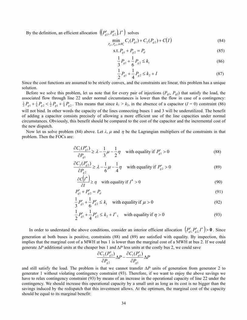
34

By the definition, an efficient allocation ( )( )∗∗∗ IPP gg ,, 21 solves

( )ICPCPC ggIPP gg

+++∈

)()(min 2211,, 321 R

(84)

dgg PPP =+ 21 s.t. (85)

121 61

31 kPP gg ≤+ (86)

IkPP gg +≤+ 221 41

21

(87)

Since the cost functions are assumed to be strictly convex, and the constraints are linear, this problem has a unique solution.

Before we solve this problem, let us note that for every pair of injections (Pg1, Pg2) that satisfy the load, the associated flow through line 22 under normal circumstances is lower than the flow in case of a contingency:

241

121

261

131

gggg PPPP +<+ . This means that since k1 > k2, in the absence of a capacitor (I = 0) constraint (86) will not bind. In other words the capacity of the lines connecting buses 1 and 3 will be underutilized. The benefit of adding a capacitor consists precisely of allowing a more efficient use of the line capacities under normal circumstances. Obviously, this benefit should be compared to the cost of the capacitor and the incremental cost of the new dispatch.

Now let us solve problem (84) above. Let λ, μ and η be the Lagrangian multipliers of the constraints in that problem. Then the FOCs are:

0 ifequality with 21

31)(

11

11 >−−≥∂

∂ ∗∗

gg

g PP

PCημλ (88)

0 ifequality with 41

61)(

22

22 >−−≥∂

∂ ∗∗

gg

g PP

PCημλ (89)

( ) 0 ifequality with >≥∂

∂ ∗∗

IIIC η (90)

dgg PPP =+ ∗∗21 (91)

0 ifequality with 61

31

121 >≤+ ∗∗ μkPP gg (92)

0 ifequality with ,41

21

221 >+≤+ ∗∗∗ ηIkPP gg (93)

In order to understand the above conditions, consider an interior efficient allocation ( ) 0>∗∗∗ IPP gg ,2,1 . Since generation at both buses is positive, constraints (88) and (89) are satisfied with equality. By inspection, this implies that the marginal cost of a MWH at bus 1 is lower than the marginal cost of a MWH at bus 2. If we could generate ΔP additional units at the cheaper bus 1 and ΔP less units at the costly bus 2, we could save

PP

PCP

PPC

g

g

g

g Δ∂

∂−Δ

∂∂ ∗∗

1

11

2

22 )()(

and still satisfy the load. The problem is that we cannot transfer ΔP units of generation from generator 2 to generator 1 without violating contingency constraint (93). Therefore, if we want to enjoy the above savings we have to relax contingency constraint (93) by means of an increase in the operational capacity of line 22 under the contingency. We should increase this operational capacity by a small unit as long as its cost is no bigger than the savings induced by the redispatch that this investment allows. At the optimum, the marginal cost of the capacity should be equal to its marginal benefit:

35

( ) PP

PCP

PPC

IIC

g

g

g

g Δ∂

∂−Δ

∂∂

=∂

∂ ∗∗∗

1

11

2

22 )()(

And this is precisely one of the implications of the first order conditions (88-91) above. To see this, note that since

I* > 0, equation (90) is satisfied with equality, and hence ( ) η=∂

∂ ∗

IIC . Since by assumption, the marginal cost of

capacitor-induced capacity is positive, η > 0, and consequently constraint (93) is binding. It can be shown that in this case μ= 0.6 On the other hand, a unit of additional capacity in case of a contingency allows us to change the injections in buses 1 and 2 by 1gPΔ and 2gPΔ , respectively, where 1gPΔ and 2gPΔ satisfy

0

141

21

21

21

=Δ+Δ

=Δ+Δ

gg

gg

PP

PP

This means that the unit of additional capacity allows us to redispatch in a way that 41 =Δ gP , and 42 −=Δ gP . The savings in the generation cost that this new redispatch induces is

η

ημ

ημλημλ

ημλημλ

=

+=

⎟⎟⎠

⎞⎜⎜⎝

⎛⎟⎠⎞

⎜⎝⎛ −−−⎟

⎠⎞

⎜⎝⎛ −−−=

Δ⎟⎠⎞

⎜⎝⎛ −−−Δ⎟

⎠⎞

⎜⎝⎛ −−−=Δ

∂∂

−Δ∂

∂−

∗∗

32

41

61

21

314

41

61

21

31)()(

2122

221

1

11ggg

g

gg

g

g PPPP

PCP

PPC

where the last equality follows from the fact that μ = 0 . Now that we have a characterization of the efficient allocation, we can ask how to implement it. One alternative

would be to impose it by a central planning committee. This entity knows what the efficient allocation is and can, in principle, dictate the optimal generation levels to the generators and the optimal capacitor-induced capacity to the investment firm. In reality, however, trying to impose an allocation to the different players may be an impossible task. One would have to know the cost structure of every generator and of the investment firms, and more importantly, one would have to have the power to impose on them the optimal generation and investment levels. Another alternative would be to decentralize the decisions by means of a price system and a competitive market. The idea of such price system is to allow the generators and investment firms to decide for themselves the generation and investment levels, respectively, taking electricity prices and transmission charges as given. The objective is still the same, but the huge task of determining the optimal allocation is now subdivided into many small tasks, each performed by each economic agent. Nobody needs to know the technology and cost structure of all the firms. It is enough for each firm to know its own cost function. Similarly, it is not needed for any omniscient central planner to figure out the optimal allocation. Each economic agent will try to maximize its own profits given the market prices. Presumably, the players will decide what is best for themselves but if the prices are right, these prices will induce the players to choose the quantities that correspond to the efficient allocation.

In the following definition of economic equilibrium, there will be electricity prices associated to each bus (the nodal prices), and two different transmission charges. Both transmission charges are related to congestion on the 1-3 corridor. One charge can be associated to the transmission on the lines under normal circumstances, and the

6Note that ( )26

113

132

241

121

gggg PPPP +=+ . Therefore, constraint (87) can be written as .132

241

121 kPP gg ≤+ If constraint (93)

is binding then ≤+=+ 241

121

2 gg PPIk 132 k and it is satisfied. Consequently, μ= 0.

36

other to the transmission under the contingency. The generators and investment firm will take these prices as given and will choose their generation and investment decisions optimally.

Definition: An allocation ( )( )∗∗∗ IPP gg ,, 21 and a price vector ( )∗∗∗∗∗ ωτπππ ,,,, 321 constitute a competitive equilibrium if the following conditions are satisfied: 1. Generators' profit maximization: each generator, Gn, for n = 1, 2, chooses its generation level ∗

gnP so as to

maximize its profits given the nodal price ∗nπ :

2,1 ,0)()( =≥∀−≥− ∗∗∗∗ nPPCPPCP gngnngnngnngnn ππ 2. Investment firm's profit maximization: the investment firm, chooses the capacitor-induced capacity I* so as to

maximize its profits given the contingency transmission charge ω*: ( ) ( ) 0≥∀−≥− ∗∗∗∗ IICIICI ωω

3. Power market clears: power supply equals the load.

dgg PPP =+ ∗∗21

4. Transmission market clear: demand for transmission, both under normal circumstances and under the contingency, should not exceed the capacity. And the associated transmission charge is positive only if demand for transmission equals capacity

0 ifequality with 41

21

0 ifequality with 61

31

221

121

>+≤+

>≤+

∗∗∗∗

∗∗∗

ω

τ

IkPP

kPP

gg

gg

5. No arbitrage conditions: it should not be possible to make a profit by buying power at one of the buses at its market price, transmitting it to another node and paying the corresponding transmission charge, and selling it there at that bus's market price:

∗∗∗∗ ++= ωτππ212

31

13 (94)

∗∗∗∗ ++= ωτππ412

61

23 (95)

In order to understand conditions (94) and (95), note that if we inject one MW at bus 1 and eject it at bus 3, under normal circumstances 1/3 of the MW will transit through line 21 and 1/3 of the MW will transit through line 22.7 If the contingency occurs, then 1/2 of the MW will transit through the remaining line 22. Therefore, each MW injected at bus 1 and ejected at bus 3 must pay 1/3 of the price of transmission along line 21and 1/3 of the price of transmission along line 22, under normal circumstances, and 1/2 of the price of transmission along line 22 under the contingency. If we add the price/hour of the MW at bus 1, we obtain that the cost of buying one MWH at bus 1 and transmitting it to bus 3 is ∗∗∗ ++ ωτπ 2

131

1 2 . The first no-arbitrage condition states that this cost

should equal the price that one would obtain by selling this MWH at the destination bus. A similar interpretation applies to no-arbitrage condition (95).

Let's characterize a competitive equilibrium. For this purpose assume that allocation ( )( )∗∗∗ IPP gg ,, 21 and a

price vector ( )∗∗∗∗∗ ωτπππ ,,,, 321 constitute a competitive equilibrium. Then the generation level ∗gnP , for n = 1, 2,

satisfies the first order conditions of the generator's profit maximization problem:

7The other third will transit through lines 1 and 3.

37

0 ifequality with )(

111

11 >≥∂

∂ ∗∗∗

gg

g PP

PCπ (96)

0 ifequality with )(

222

22 >≥∂

∂ ∗∗∗

gg

g PP

PCπ (97)

Also, the investment firm capacitor-induced capacity satisfies the first order conditions of its profit maximization problem:

( ) 0>≥∂

∂ ∗∗∗

ity if Iwith equalωIIC (98)

As a result, a competitive equilibrium is characterized by conditions (96-98) and the market clearing and nor-arbitrage conditions above.

By comparison, we can see that if allocation ( )( )∗∗∗ IPP gg ,, 21 solves the social optimum problem (84) with

associated Lagrangian multipliers λ, μ and η, then the same allocation ( )( )∗∗∗ IPP gg ,, 21 together with the price

vector ( )∗∗∗∗∗ ωτπππ ,,,, 321 defined by

ηω

μτ

λπ

ημλ

ημλ

=

=

=

−−=

−−=

∗

∗

∗

∗

∗

2/

41

61

21

31

3

2

1

g

g

P

P

is a competitive equilibrium. Conversely, if allocation ( )( )∗∗∗ IPP gg ,, 21 together with price vector

( )∗∗∗∗∗ ωτπππ ,,,, 321 constitute a competitive equilibrium, then the same allocation ( )( )∗∗∗ IPP gg ,, 21 together with the Lagrangian multipliers defined by

∗

∗

=

=

=

ωη

τμ

πλ

23

solve the social optimum problem (84).

The above analysis shows that the competitive equilibrium leads to the efficient allocation. In particular, the competitive equilibrium induces the optimal amount of capacitor-induced capacity enhancement. 3.6 SUMMARY The transmission planning process is receiving a great deal of attention today because it is arguably the most significant technical element of competitive electric markets for which consensus has not yet been reached in regards to its implementation. Impediments to achieving that consensus include difficulties in siting and obtaining right-of-ways, the significant investment cost, uncertainties associated with predicting future information affecting network operation, and difficulties in identifying beneficiaries, assignment of cost responsibilities, and how cost recovery takes place for investors. Some organizations have provided answers to these questions, and those answers for one such organization are summarized in this document. We also provide a general optimization framework for transmission planning, and we illustrate its use for two difference cases; when solutions are restricted to new circuits only, and when solutions are restricted to switchable shunt and series capacitors only. Although the latter case cannot always be implemented alone, it is economically attractive when it is a feasible

38

solution. We provide a detailed description and illustration of practical optimization procedures for identifying optimal location and amount of switchable shunt and series capacitors to increase contingency-limited transmission capacity through network reconfiguration. This approach is attractive because it is conceptually based on the automaton, a key element in addressing dynamic performance for discrete-event systems. We describe our implementation of system design, in terms of sequence and timing of configurable switches, based on identification of stability regions corresponding to the considered switching mode. The last part of our chapter focuses on the efficiency of the electricity market with inclusion of the facility investment effects. The interesting conclusion is that, when transmission expansion is limited to contingency-driven switchable capacitors, the competitive equilibrium leads to the efficient allocation. ACKNOWLEGMENTS The authors express appreciation to Qiming Chen and John Condren of PJM Interconnection for the helpful suggestions related to Section 3.2 of this material, and to John Paserba of Mitsubishi Electric Power Products, Inc. for his careful review and helpful comments throughout the paper. REFERENCES [1] M. Buygi, G. Balzer, H. Shanechi, and M. Shahidehpour, “Market-based transmission expansion planning,” IEEE Transactions On Power Systems, Vol. 19, No. 4, November 2004, pp. 2060-2067. [2] E. Hirst, “U.S. Transmission Capacity: Present Status and Future Prospects,” 2004, at www.ee.iastate.edu/~jdm/ee458/TransmissionCapacityFinal_Herst.pdf. [3] M. Shahidehpour, “Investing in expansion: the many issues that cloud transmission planning,” IEEE Power and Energy Magazine, Jan/Feb. 2004, pp. 1-18. [4] L. Dale, “Reactive compensation using static VAR compensators-a planning case study using security constrained techniques,” International Conf. on AC and DC Power Transmission, Sept. 17-20, 1991, pp. 50 – 54. [5] R. Koessler, J. Mountford, L. Lima, and J. Rosende, “The Brazilian interconnected system: a study on transfer limits, reactive compensation and voltage collapse,” Proc. of the IEEE Power Engineering Society Winter Meeting, Vol. 3, Jan. 28-Feb. 1, 2001 pp. 1147 – 1153. [6] P. Pourbeik, R. Koessler, and B. Ray, “Tools and techniques for analyzing voltage stability related reliability challenges,” Proc. on the IEEE Power Engineering Society Transmission and Distribution Conference and Exposition, Vol. 1, Sept. 12 2003,pp. 417 – 421. [7] A. Hammad and M. El-Sadek, “Prevention of transient voltage instabilities due to induction motor loads by static VAr compensators,” IEEE Transactions on Power Systems, Vol. 4, Issue 3, Aug. 1989, pp. 1182 – 1190. [8] M. S. Branicky, ``Modeling Analysis and Control of Hybrid Systems'', PhD Thesis Massachusetts Institute of Technology, 1994. [9] Tomlin, C.J.; Lygeros, J.; Shankar Sastry, S.; “A game theoretic approach to controller design for hybrid systems,” Proceedings of the IEEE, Volume: 88 Issue: 7 , Jul 2000 , Page(s): 949 -970 [10] “Regional Transmission Organizations,” Docket No. RM99-2-000; Order 2000 of the Federal Energy Regulatory Commission (FERC), issued Dec. 20, 1999; www.ferc.gov/legal/ferc-regs/land-docs/RM99-2A.pdf. [11] www.ferc.gov/industries/electric/indus-act/rto.asp [12] Final Rule - Order 2003, “Standardization of Generator Interconnection Agreements and Procedures,” Docket No. RM02-1-000, Issued July 24, 2003. [13] “Flow Chart of the Large Generating Facility Interconnection Process,” in Appendix A to the Final Rule - Order 2003 “Standardization of Generator Interconnection Agreements and Procedures.” [14] Schedule 6 of “Operating agreement of PJM Interconnection L.L.C.,” June 22, 2005, at www.pjm.com/documents/agreements.html. [15] “PJM Manual 14B: Generation and Transmission Interconnection Planning,” Revision: 05, June 23, 2005, at www.pjm.com/contributions/pjm-manuals/manuals.html. [16] T. Wu, Z. Alaywan, A. Papalexopoulos, “Locational Marginal Price Calculations Using the Distributed-Slack Power-Flow Formulation,” IEEE Transactions On Power Systems, Vol. 20, No. 2, May 2005. [17] “PJM Manual 27: Open Access Transmission Tariff Accounting Revision,” Revision 46, May 01,2005 at www.pjm.com/contributions/pjm-manuals/manuals.html. [18] “PJM Manual 06: Financial Transmission Rights,” Revision 7, April 15, 2005, at www.pjm.com/contributions/pjm-manuals/manuals.html. [19] F. Schweppe, M. Caramanis, R. Tabors, and R. Bohm, “Spot Pricing of Electricity,” Boston, Kluwer Academic Press, 1988.

39

[20] N. Rau, “Optimization principles: practical application to the operation and markets of the electric power industry,” John Wiley, 2003. [21] D. Kirschen and G. Strbac, “Power system economics,” John Wiley, 2004. [22] “Operating agreement of PJM Interconnection, L.L.C.,” June 22, 2005, at http://www.pjm.com/documents/downloads/agreements/. [23] P. Jaskow, “Transmission Policy In The United States,” Utilities Policy, 13: 95-115, 2005. at http://econ-www.mit.edu/faculty/download_pdf.php?id=1003 [24] New York Independent System Operator, “Transmission Expansion and Interconnection Manual,” September 1999, at http://www.nyiso.com/public/documents/manuals/planning.jsp. [25] ISO New England Planning Procedures, at http://www.iso-ne.com/rules_proceds/isone_plan/index.html. [26] Z. Alaywan, “Understanding the California Firm Transmission Rights,” at www.caiso.com/aboutus/articles/. [27] Z. Alaywan and T. Wu, “Effects of Firm Transmission Rights on Transmission Revenue Allocation in California,” at www.caiso.com/aboutus/articles/. [28] S. Jones, “ERCOT ISO Experience with Transmission Operating and Planning Criteria in a Competitive Environment,” Proc. of the 1999 IEEE Power Engineering Society Summer Meeting, Vol. 1, July 18-22, 1999, pp. 140–142. [29] Public Utilities Commission of Texas, P.U.C. SUBST. R. 25.101, “Transmission Planning, Licensing and Cost-Recovery for Utilities within the Electric Reliability Council of Texas,” Effective data, April 13, 2005. [30] “Midwest ISO Transmission Expansion Plan (MTEP) 2005,” June 2005, at www.midwestiso.org/plan_inter/expansion.shtml [31] “American Transmission Company 2004 10-Year Assessment Update,” March 2005, at www.atcllc.com/IT2b.shtml. [32] “American Transmission Company Planning Criteria,” Document number PLG-CR-0001-v08, July 5, 2005. [33] S. Harvey, W. Hogan, and S. Pope, “Electricity Market Design and Structure: Working Paper on Rate and Transition Issues in Standardized Transmission Service and Wholesale Electric Market Design,” Submission to the Federal Regulatory Commision, Docket No. RM01-12-000, May, 2002. [34] E. Hirst and B. Kirby, “Transmission Planning and the Need for New Capacity,” at http://certs.lbl.gov/NTGS/ISSUE_4.PDF. [35] F. Woolf, “Global Transmission Expansion; Recipes for Success,” 2003 by Penn Well Corporation, Tulsa Oklahoma. [36] Standards of the North American Reliability Council, located at www.nerc.com/~filez/pss-psg.html. [37] “NERC Planning Standards,” Section I System Adequacy and Security, Standard S1. [38] “System Protection Schemes in Power Networks,'' by Task Force 38.02.19, chaired by Daniel Karlsson and Xavier Waymel, A technical brochure for International Conference on Large High Voltage Electric Systems (CIGRE), January, 2001. [39] W. Mittelstadt, C. Taylor, M. Klinger, J. Luini, J. McCalley, and J. Mechenbier, “Voltage Instability Modeling and Solutions As Applied to the Pacific Intertie,” International Conference on Large High Voltage Electric Systems (CIGRE), June 1990. [40] N. Miller, R. D'Aquila, K. Jimma, M. Sheehan, G. Comegys, “Voltage stability of the Puget Sound system under abnormally cold weather conditions,” IEEE Trans. on Power Systems, Vol. 8, Issue 3, Aug. 1993, pp. 1133 – 1142. [41] R. L. Sullivan, Power System Planning. New York: McGraw-Hill, 1977. [42] X. Wang and J. R. McDonald, Modern Power System Planning. London: McGraw-Hill, 1994. [43] G. Latorre, R. D. Cruz, J. M. Areiza, and Andres Villegas, “Classification of Publications and Models on Transmission Expansion Planning,” IEEE Trans. Power Syst., vol. 18, pp. 938-946, May 2003. [44] V. Ajjarapu and C. Christy, “The continuation power flow: a tool for steady state voltage stability analysis,” IEEE Trans. Power Syst., vol. 7, pp. 416-423, Feb. 1992. [45] C. A. Canizares and F. L. Alvarado, “Point of collapse and continuation methods for large AC/DC systems,” IEEE Trans. Power Syst., vol. 8, pp. 1-8, Feb. 1993. [46] H. D. Chiang, A. J. Flueck, K. S. Shah, and N. Balu, “CPFLOW: a practical tool for tracing power system steady-state stationary behavior due to load and generation vacations,” IEEE Trans. Power Syst., vol. 10, pp. 623-634, May 1995. [47] S. Greene, I. Dobson, F. L. Alvarado, “ Contingency ranking for voltage collapse via sensitivities from a single nose curve,” IEEE Trans. Power Syst., vol. 14, pp. 232-240, Feb. 1999. [48] M. Ni, J. McCalley, V. Vittal, S. Greene, C. Ten, V. S. Ganugula, and T. Tayyib, “Software implementation of online risk-based security assessment,” IEEE Trans. Power Syst., vol. 18, pp. 1165-1172, Aug. 2003. [49] O. O. Obadina and G. J. Berg, “Var planning for power system security,” IEEE Trans. Power Syst., vol. 4, pp. 677-686, May 1989. [50] K. H. Abdul-Rahman and S. M. Shahidehpour, “Application of fuzzy sets to optimal reactive power planning with security constraints,” IEEE Trans. Power Syst., vol. 9, pp. 589-597, May 1994. [51] V. Ajjarapu, P. L. Lau, and S. Battula, “An optimal reactive power planning strategy against voltage collapse,” IEEE Trans. Power Syst., vol. 9, pp. 906-917, May 1994.

40

[52] J. A. Momoh, S. X. Guo, E. C. Ogbuobiri, and R. Adapa, “The quadratic interior point method solving power system optimization problems,” IEEE Trans. Power Syst., vol. 9, pp. 1327-1336, Aug. 1994. [53] K. Y. Lee, X. Bai, and Y. M. Park, “Optimization method for reactive power planning by using a modified simple genetic algorithm,” IEEE Trans. Power Syst., vol. 10, pp. 1843-1850, Nov. 1995. [54] E. Vaahedi, Y. Mansour, C. Fuchs, S. Granville, M. L. Latore and H. Hamadanizadeh, “Dynamic security constrained optimal power flow/Var planning,” IEEE Trans. Power Syst., vol. 16, pp. 38-43, Feb. 2001. [55] W. D. Rosehart, C. A. Canizares, and V. H. Quintana, “Effect of detailed power system models in traditional and voltage-stability-constrained optimal power flow problems,” IEEE Trans. Power Syst., vol. 18, pp.27-35, Feb. 2003. [56] N. Yorino, E. E. El-Araby, H. Sasaki, and S. Harada, “A new formulation for FACTS allocation for security enhancement against voltage collapse,” IEEE Trans. Power Syst., vol. 18, pp. 3-10, Feb. 2003. [57] Z. Feng, V. Ajjarapu, and D. Maratukulam, “A comprehensive approach for preventive and corrective control to mitigate voltage collapse,” IEEE Trans. Power Syst., vol. 15, pp. 791-797, May 2000. [58] I. Dobson and L. Lu, “Computing an optimal direction in control space to avoid saddle node bifurcation and voltage collapse in electrical power systems,” IEEE Trans. Automatic Control, vol. 37, pp. 1616-1620, Oct. 1992. [59] S. Greene, I. Dobson, and F. L. Alvarado, “Sensitivity of the loading margin to voltage collapse with respect to arbitrary parameters,” IEEE Trans. Power Syst., vol. 11, pp. 845-850, May 1996. [60] B. Long and V. Ajjarapu, “The sparse formulation of ISPS and its application to voltage stability margin sensitivity and estimation,” IEEE Trans. Power Syst., vol. 14, pp. 944-951, Aug. 1999. [61] G. L. Nemhauser and L. A. Wolsey, Integer and Combinatorial Optimization. New York : Wiley, 1988. [62] IEEE/CIGRE joint task force on stability terms and definitions, “Definition and classification of power system stability,” IEEE Trans. on Power Syst., vol. 19, pp. 1387-1401, Aug. 2004. [63] C. W. Taylor, Power System Voltage Stability. EPRI Power System Engineering Series. New York: McGraw Hill, 1994. [64] T. Van Cutsem and C. Vournas, Voltage Stability of Electric Power Systems. Boston: Kluwer Academic Publishers, 1998. [65] A. M. Abed, “WSCC voltage stability criteria, undervoltage load shedding strategy, and reactive power reserve monitoring methodology,” in Proc. IEEE Power Eng. Soc. Summer Meeting, vol. 1, 1999, pp. 191 – 197. [66] P. M. Anderson and A. A. Fouad, Power System Control and Stability, 2nd ed. Piscataway, N.J.: IEEE Press; Wiley-Interscience, 2003. [67] H.K.Khalil, “Nonlinear Systems,” Third Edition, Prentice Hall, New Jersey, 2002. [68] P. Varaiya, F. Wu, and R. Chen, “Direct methods for transient stability analysis of power systems: recent results,” Proceedings of IEEE, volume 73, pages 1703-1715, 1985. [69] J. Zaborszky, J. Huang, B. Zheng, and T. Leung, “On the phase portraits of a class of large nonlinear dynamic systems such as the power systems,” IEEE Transaction on Automatic Control, 33:4-15, 1988. [70] H. Chiang, M. Hirch, and F. Wu, “Stability regions of nonlinear autonomous dynamic systems,” IEEE Transactions on Automatic Control, 33:16-27, 1988. [71] H. Chiang and F. Wu, “Foundations of the potential energy boundary surface method for power system transient stability analysis,” IEEE Transactions on circuits and systems, 35:712-728, 1988. [72] V. Venkatasubramanian and W. Ji, “Numerical approximation of (n-1)-dimensional stable manifolds in large systems such as power system,” Automatica, 33:1877-1883, 1997. [73] D. Cheng and J. Ma, “Calculation of stability region,” Proceedings of the 42nd IEEE conference on decision and control, volume 6, pages 5615-5620, maui, Hawaii,USA, 2003. [74] S. Saha, A. A. Fouad, W. H. Kliemamm, and V. Vittal, “Stability boundary approximation of a power system using the real normal form of vector fields,” IEEE Transaction on Power Systems, 12:797-802, 1997. [75] R. Qi, D. Cook, W. Kliemann, and V. Vittal, “Visualization of stable manifolds and multidimensional surfaces in the analysis of power system dynamics,” Journal of Nonlinear Science, 10:175-195, 2000. [76] N. Anthony, A. Fouad, and V. Vittal, “Power system transient stability using individual machine energy functions,” IEEE Transaction on Circuits and Systems, 30:266-276, 1983. [77] M. Ribbens-Pavella and F. Evans, “Direct methods for studying dynamics of large scale power system - a survey,” Automatica, 32:1-21, 1985. [78] H. Chiang and J. Thorp, “The closest unstable equilibrium point method for power system dynamic security assessment,” IEEE Transaction on Circuits and Systems, 36:1187-1199, 1989. [79] L. Jin, H. Liu, R. Kumar, V. Ajjarapu, J. McCalley, N. Elia, and V. Vittal, “An application of reachable set analysis in power system transient stabiltiy assessment,” Proceedings of the 2005 IEEE PES General Meeting, San Francisco, June 2005. [80] I. M. Mitchell, “Application of level set methods to control and reachability problems in continuous and hybrid systems,” PhD thesis, Stanford University, Stanford, 2002.

41

[81] H. Liu, L. Jin, V. Ajjarapu, R. Kumar, J. McCalley, N. Elia, and V. Vittal, “Reachability analysis based minimal load shedding determination,” Proceedings of the 2005 IEEE PES General Meeting, San Francisco, June 2005. [82] W. W. Hogan, “Contract Network for Electric Power Transmission,” Journal of Regulatory Economics, 4:211-242, 1996. [83] J. B. Bushnell and S. E. Stoft, “Electric Grid Investment Under a Contract Network Regime,” Journal of Regulatory Economics, 10:61-79, 1996. [84] Chao, Hung-Po and Peck, Stephen, 1996. "A Market Mechanism for Electric Power Transmission," Journal of Regulatory Economics, Springer, vol. 10(1), pages 25-59. [85] J. B. Bushnell and S. E. Stoft, “Improving Private Incentives For Electric Grid Investment,” Resource and Energy Economics, 19:85-108, 1997. [86] P. Joskow and J. Tirole, “Merchant Transmission Investment,” Journal of Industrial Economics. Volume 53, Issue 2, pp. 233-264, June 2005.