Chapter 3 - Magnetics

8/8/2019 Chapter 3 - Magnetics

http://slidepdf.com/reader/full/chapter-3-magnetics 1/10

Chapter 3 – Magnetic Fields

Chapter 3 – Magnetic Fields ............................................................................................................................ 1

3.1 Introduction ...................................................................................................................................... 2

3.2 Electric Fields – Electrostatics ......................................................................................................... 2

3.2.1 Relationships ................................................................................................................................ 23.2.2 Permittivity .................................................................................................................................. 2

3.3 Magnetic Fields ............................................................................................................................... 3

3.3.1 Relationships ................................................................................................................................ 33.3.2 Permeability ................................................................................................................................. 3

3.3.3 Magnetization curve .................................................................................................................... 5

3. 4 Intensity & Density .......................................................................................................................... 63.5 Motor & Generator .......................................................................................................................... 6

3.5.6 Hysteresis and eddy currents ....................................................................................................... 7

3.6 Mechanical motion .......................................................................................................................... 8

3.6.1 Relationships ................................................................................................................................ 8

3.6.2 Gravity ......................................................................................................................................... 83.6.3 Linear v. rotational....................................................................................................................... 8

3.7 Mathematical manipulation ............................................................................................................. 9

3.8 Maxwell ........................................................................................................................................... 93.9 Exemplars ...................................................................................................................................... 10

3.10 Applications ................................................................................................................................... 10



2 Electric Power Concepts Durham

3.1 Introduction

Circuits are based on the elements constrained to a solid structure. Fields are analogous to a gas where the

performance is distributed through space.

3.2 Electric Fields – Electrostatics

3.2.1 Relationships

Electric fields are the result of a charge. When the charge is measured from a point or node it is called statics. Whenthe charge is dispersed in space like a gas the energy is called a dynamic field.

A capacitor is simply two electrically charged conductors that are separated by a dielectric. Energy relationships are

used to convert between electric, magnetic, and mechanical systems.

The fundamental relationships for an electric field are listed.

(energy) W Fs Vq NI energy conversion

(closed loop) 2s r

(electric intensity) V/meter F V

q sE

2Coulomb(electric density)

q A m

D E

q = charge

1 electron = 1.6021x10-19

Coulomb

3.2.2 Permittivity

Permittivity is the dielectric or charge insulation material property.

r o

9136 10

o

Farad/m

Force occurs on charge 2 due to charge 1.

1 2

2

4

q qF

r

Electric field intensity at point 2 is due to point charge at point 1.

1

24

qF

q r E

A radial electric field comes from a line charge on the z-axis.

2

L

r

E



Chapter 3 Magnetics 3

PAGE 3

coulombline charge density -

m L

A plane electric field arises from a sheet charge in x-y plane.

2

s

E

2

coulombsheet charge density -

ms

Energy is dependent on the electric field, which can be converted to voltage.

2

2

1

2

1

2

W q s

W qV CV

E D

3.3 Magnetic Fields

3.3.1 Relationships

Magnetic fields are the result of a pole or flux. When the pole strength is measured from a point or node it is called

statics. When the magnetics are dispersed in space like a gas the energy is called a dynamic field.

An inductor is simply is simply a coil of wire that creates a magnetic field. Energy relationships are used to convert

between electric, magnetic, and mechanical systems.

The fundamental relationships for magnetic devices are listed.

(energy) W Fs Vq NI energy conversion

(closed loop) 2s r

(magneto-motive force) mmf = Amp-turns NI H dl F R

F(magneticintensity) Amp/m

NI

s H

2Weber(field density)

m H

A

B

2

(reluctance)l N

A L R

3.3.2 Permeability

Permeability is the magnetic property of material.

r o

74 10 Henry/m

o

i

N

l

Air gap

lg

A –

crosssectional area




(copper) 2r

(amorphoussteel) 2000r (laminated steel) 6000r

Force occurs on pole 2 due to pole 1.

1 2

2

4

F

r

(fluxlinkage) n LI

EXAMPLES

3.1 Given: Laminated iron core

depth of core .05 m

width of core .05 m

length of air gap .0007 m

effective length of core 0.3 m

relative permeability of Fe 2000

air gap flux density 0.5 T

number of turns 200

Find:

a. total flux (include flaring at air gap)

0.5 .05 .05 0.00125

1.05 0.0013125 Wb AIR

B A

BA

b. flux density in the iron

2

1.05

0.5 1.05 0.525 Wb/m

Fe AIR

Fe

B B

B

c. magnetic intensity in the iron

0

7208.82 A/m

2000 4 10

1.05 0.0013125 Wb

r

AIR

B H

B B H

B H

d. total mmf required on the core

0.3 62.66 A-turnsmmf NI Hlmmf H

e. current required on the core

62.66A

200

mmf NI

mmf I

N




PAGE 5

3.3.3 Magnetization curve

The magnetic circuit for a machine includes the current and turns, the ferromagnetic metal, and air gaps.

The magnetization curve shown below is a non-linear relationship for the magnetic circuit, and is typical of all

magnetic circuits. It is used to show the conversion between representations of magnetic energy.

0

50

100

150

200

250

300

350

0 2000 4000 6000 8000 10000 12000

The first portion of the curve has a physical anomaly near zero. The portion less than 5000 is in the unsaturated

region. There is an approximate proportional change in the vertical axis as the horizontal changes. About 5000 is

called the knee. That is the transition region. The top portion of the curve above about 5000 is the saturated region.

There is very little change in the vertical parameter as the horizontal is increased.

The values are strictly representative. Different material alloys will yield other range of values. Nevertheless, thegeneral shape and form can be used for a variety of problems.

The curve then can represent a number of different relationships. Some of the more common are shown in the table

below.

X-axis name unit Y-axis name unit Curve name unit

F mmf A-turns flux Weber R reluctance

H intensity A-turns/m B density Wb/m2 µ permeability H/m

I field I Amps V terminal Volts synchronous

F field mmf A-turns Ea Internal gen Volts dc machine

EXAMPLES

3.1 Given: Magnetization curve shown above

Find:

a. For an intensity H of 5000, what is the density B?

Read chart along bottom to 5000.

Read vertical to curve.

Read result on left column of 250

b. For a density B of 250 what is the relative permeability?




2500.05

5000

B H

B

H

c. For a flux of 250, what is the mmf?

Read left column to 250

Read right to curveRead result down to 5000

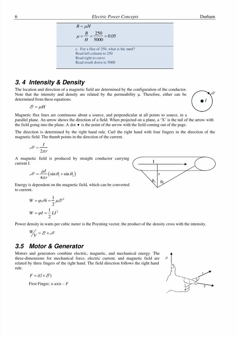
3. 4 Intensity & Density The location and direction of a magnetic field are determined by the configuration of the conductor.

Note that the intensity and density are related by the permeability μ. Therefore, either can bedetermined from these equations.

H B

Magnetic flux lines are continuous about a source, and perpendicular at all points to source, in a

parallel plane. An arrow shows the direction of a field. When projected on a plane, a ‘X’ is the tail of the arrow withthe field going into the plane. A dot is the point of the arrow with the field coming out of the page.

The direction is determined by the right hand rule. Curl the right hand with four fingers in the direction of the

magnetic field. The thumb points in the direction of the current.

2

I

r H

A magnetic field is produced by straight conductor carrying

current I.

1 2sin sin

4

I

r

H

Energy is dependent on the magnetic field, which can be converted

to current.

2

2

1

2

1

2

W s

W I LI

H B

Power density in watts per cubic meter is the Poynting vector, the product of the density cross with the intensity.

W

V B H

3.5 Motor & Generator Motors and generators combine electric, magnetic, and mechanical energy. The

three-dimensions for mechanical force, electric current, and magnetic field are

related by three fingers of the right hand. The field direction follows the right hand

rule.

( )F i l B

First Finger, x-axis – F

B

I

F

r

θ1 θ2

I

H

I




PAGE 7

Middle Finger, y-axis – I, length, velocity

Thumb, z-axis – B

In another application of the right hand rule, with the fingers curled in the direction of current, the thumb will point in

the direction of the magnetic flux, φ.

The motor relationship comes from an electric current flow through a magnetic field. This creates a mechanical force

( )F i l B

( )F q v B

The generator relationship comes from a wire moving through a field. This creates an electrical voltage.

(voltage) ( ) e v lB

Since voltage and current are not traditionally considered vectors,

the length of the line carrying the current is used for the direction.

The cross-product vector directions are determined by the curl of

the right hand. Start with the fingers of the hand pointing in the

direction of the first vector. With the hand curling from one vector

toward the second vector direction, the cross-product result is inthe direction of the thumb. The dot product is in the same direction

as the two vectors.

3.5.6 Hysteresis and eddy currents

The non-linear nature of magnetic devices creates some rather interesting phenomenon. The non-linear characteristic

of a magnet causes it to follow different path when the magnet is being

energized and when it is de-energized. This alternative trace is calledhysteresis.

Hysteresis is the lag between cause and effect. The system does notinstantly respond to the energy applied to it. Rather the system reacts

slowly, or does not return completely to its original state. The system’sstate depends on the immediate history. For example, when pressed putty

will assume a new shape, and when the pressure is removed it will not

return to its original shape immediately and entirely.

It is hysteresis or residual magnetism that causes data to be stored on a magnetic tape and hard disks. The residual

magnetism is also used to get a generator working. In motors, which repeatedly are energized and de-energized,

hysteresis causes loss and reduces efficiency.

Another phenomenon of magnetic systems is eddy current. Like the eddy pools in a

flowing stream, these are small swirls of current that oppose change in energy. Eddy

currents develop on magnetic materials, such as steel, because of anomalies in the

molecular structure. To keep the eddy currents from becoming large, the steel core is made

in thins layers. Alternatively in some systems, slits may be cut in the steel core.

Eddy currents are used to create dynamic braking. In motors which are continually

energized and de-energized, eddy currents causes loss and reduces efficiency.




3.6 Mechanical motion

3.6.1 Relationships

Mechanical motion is the result of mass. When the mass is measured from a point or node it is called statics. When

the mass is in motion it is call dynamics. Energy relationships are used to convert between electric, magnetic, and

mechanical systems.

The fundamental relationships for three types of field are listed.

W(Energy) Fs Vq NI energy conversion

W P

t power

3.6.2 Gravity

Gravity constant is the mass property of material.

10 2 28.38 10 /

o

N m kg

Force occurs on mass 2 due to mass 1.

1 2

24

m mF

r

Energy is dependent on the mass field.

F ma

W Fs mas

2

2

2

12

potential energy

average kinetic energy

instanteous kinetic energy

total energy conversion

W mgh

W mv

W mv

W mc

3.6.3 Linear v. rotational

The motion of mass has both linear and rotational properties. Because of the rotation of machines, the angular

calculations are more common.

Name Linear Units Angular Units

displacement s meter θ radian

velocity v=s/t m/sec ω= θ/t rad/sec

acceleration a=v/t m/sec2 α= ω/t rad/sec

2

mass m kilogram moment of inertia J kg-m2

force F=ma Newton torque via angular T =J α Nt-m

torque via linear T =s x F Nt-m

energy W=s·F Joule W= T θ Joule

power P=Fv Watt P= T ω Watt




PAGE 9

3.7 Mathematical manipulation Numerous equations and relationships have been broached in this chapter. These are the basis for most electrical,

magnetic, and mechanical machine analysis. The study requires manipulation of relationships in a variety of ways

and combinations.

There is a simple technique for systematic manipulation: Begin with a known quantity. Draw a horizontal line so the

units can be manipulated until the correct form is obtained. Then the equation will be correct, except for conversion

constants.

As an example, convert revolutions per minute (RPM) to radians per second.

rev min 2 radrad/sec

min 60sec rev 30

3.8 Maxwell Maxwell’s Equations are a summary of all that is electrical and magnetic in a Calculus form. Although they are no

easily used, they do provide a mathematically clever summary. The integral form is tedious, but the point form

supplies definitions.

0

B E t

D H J t

D

E

The del is the three-dimensional partial derivative with respect to the x, y, and z axes.

The electric-magnetic energy equation contains all the information in one equation[1]. Note that all the definitions

are in the point equation. In addition, all the field information is in the distributed equation. W is energy and V is

volume in these equations.

z yqW

t

z y ys t y

r y

q b d sW

t V

axial distance

radial distance

rotational distance

s

b

d

Realizing the orthogonal nature of the fields, the equations inherently contain the directions and require only vectoralgebra.

[1] "A Composite Approach to Electrical Engineering," Marcus O. Durham, Institute of Electrical and Electronic

Engineers Region V , 88CH25617-6/000-143, Colorado Springs, CO, March 1988, pp 143-147.

Applications Engineering Approach to Maxwell and Other Mathematically Intense Problems“, Marcus O. Durham

Robert A. Durham, and Karen D. Durham, Institute of Electrical and Electronics Engineers PCIC , September 2002.

"Applications Engineers Don't Do Hairy Math", Marcus O. Durham, Robert A. Durham, and Karen D. Durham

Proceedings of 35th Annual Frontiers in Power Conference, OSU, Stillwater, OK, October 2002.




"Electromagnetics in One Equation Without Maxwell", Marcus O. Durham, American Association for Advancement

of Science - SWARM , Tulsa, OK, April 2003.

3.9 Exemplars An exemplar is typical or representative of a system. These examples are representative of real world situations.

3.10 Applications Applications are an opportunity to demonstrate familiarity, comfort, and comprehension of the topics.

Application 5-1SITUATION:

Chapter 3 - Magnetics

Documents

Transcript of Chapter 3 - Magnetics