Chapter 3

Expert System and Knowledge-based Artificial Neural

Network

Expert Systems such as Mycin, Dendral, Prospector, Caduceus,

etc., proved to be successful in early eighties. In late

eighties success of the Neural Network (NN) approach to

problems such as learning to speak [Sejnowski and Rosenberg

1986], medical reasoning [Gallant 1988], recognizing

handwritten characters, [Mui and Agarwal 1993; Baxt 1992; Wang

1991; Bottan and Vapnik 1992; Hoffman et.al 1993; Nagendra

Prasad et.al 1993] etc., gave a new impetus to research in

Neural Computing. The neural network approach has been an

increasingly important approach to artificial intelligence

[Feldman and 3allard 1982; Rumelhart et al. 1986; Smolensky

1987; Feldr.an et al. 1988]. The Neural Network approach is

being applied to difficult, A.I. problems. Fu and Fu [1990]

suggested a novel approach wherein a rule-based conventional

expert system was mapped into a neural architecture in both

the structural and behavioral aspects. It was suggested that

the NN approach can enhance the performance of Conventional

Expert Systems (CES).

The Neural Network approach contrasts with the

knowledge-based approach in several aspects. The knowledge of

a neural network lies in its connections and associated

weights, whereas the knowledge of a rule-based system lies in

rules. A neural network processes information by propaga-ting

and combining activations through the network, but a

knowledge-based system (Fig. 1) reasons through symbol

generation and pattern matching. The knowledge-based

55

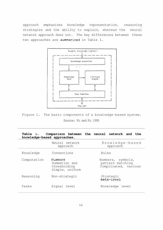
approach emphasizes knowledge representation, reasoning

strategies and the ability to explain, whereas the neural

network approach does not. The key differences between these

two approaches are summarized in Table 1.

Figure 1. The basic components of a knowledge-based system.

Source: Fu and Fu 1990

56

Table l. Comparison between the neural network and theknowledge-based approaches.

Neural network Knowledge-basedapproach approach

Knowledge Connections Rules

Computation Numbers Numbers, symbols,Summation and pattern matchingthresholding Complicated, variousSimple, uniform

Reasoning Non-strategic Strategicmeta-level

Tasks Signal level Knowledge level

3.1 Mapping Rule-based Systems intoNeural Architecture

A rule-based system (knowledge represented in rules) can be

transformed into an inference network where each connection

corresponds to a rule and each node corresponds to the premise

or the conclusion of a rule, as seen in Figure 2. Reasoning

Figure 2. An inference network.

Source: Fu and Fu 1990

in such systems is a process of propagating and combining

multiple pieces of evidence through the inference network

until final conclusions are reached. Uncertainty is often

handled by adopting the certainty factor (CF) or the

probabilistic schemes which associate each fact with a number

called the belief value. An important part of reasoning

tasks is to determine the belief values of the pre-defined

final hypothesis given the belief values of observed

evidence. The network of an inference system through which

belief values of evidences or hypotheses are propagated and

57

combined is called the belief network. Correspondence in

structural and behavioral aspects exists between neural

networks and belief networks, as shown in Table 2. For

instance, the summation function in neural networks

corresponds to the function for the Bayesian fomula for

deriving posterior probabilities in PROSPECTOR-like systems.

The thresholding function in neural networks corresponds to

predicates such as SAME (in Mycin-like systems), which cuts

off any certainty value below 0.2.

Since belief network corresponds to neural network by

mapping the knowledge base and the inference engine into a

kind of neural network called conceptualization, which stores

knowledge and performs inference and learning. Furthermore,

to construct a conceptualization, the following mappings need

to be done.

• Final hypotheses are mapped into output neurons (neurons

without connections pointing outwards),

• Data attributes are mapped into input neurons (neurons

without connections pointing outwards),

58

Table 2. Correspondence between neural networks and beliefnetworks.

Neural networks Belief networks

Connections RulesNodes Premises, conclusionsWeights Rule strengthsThresholds PredicatesSummation Combination of belief

values

Propagation of activations Propagation of beliefvalues

• Concepts that summarize or categorize subsets of data or

intermediate hypotheses that infer final hypotheses are

mapped into middle (also known as hidden) neurons, and

• The strength of a rule is mapped into the weight of the

corresponding connection.

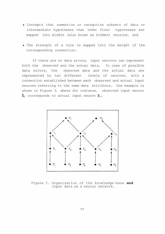
If there are no data errors, input neurons can represent

both the observed and the actual data. In case of possible

data errors, the observed data and the actual data are

represented by two different levels of neurons, with a

connection established between each observed and actual input

neurons referring to the same data attribute. One example is

shown in Figure 3, where for instance, observed input neuron

E, corresponds to actual input neuron E,.

Figure 3. Organization of the knowledge-base andinput data as a neural network.

59

3.2 Knowledge Representation

In this section the knowledge representation language in MYCIN

[Buchanan and Shortliffe 1934] or similar systems is reviewed.

The issue of how to map such language into conceptualization

is then examined, and knowledge representation of the neural

network is described.

In MYCIN, facts are represented by context-attribution

(or object-attribute-value) triples. Each triple is a term.

For instance, the term 'throat which is the site of the

culture1 is represented by the triple <CULTURE SITE THROAT>.

Each triple is associated with certainty factor, which is

described later.

A sentence is represented by predicate-context-

attribute-value quadruple. For instance, the sentence 'the

site of the culture is throat1 is represented by quadruple

<SAME CULTURE SITE THROAT>. The truth value of a sentence is

determined by whether the triple satisfies the predicated in

terms of its CF.

Judgmental and inferential knowledge is represented in

production rules; i.e., if-then rules. If a rule's IF-part

is evaluated to be true, its THEN part will be concluded.

Each part is constituted by a small nur.ber of sentences. For

instance, a MYCIN rule.

*RULE 12 4

IF:

1. The site of the culture is throat.

2. The identity of the organism is Streptococcus.

THEN: There is strongly suggestive evidence (.8)

that the subtype of the organism is not group-D.

60

can be encoded in MYCIN language as

*(RULE 124 (($AND(SAME CULTURE SITE THROAT)

(SAME ORGANISM IDENTITY STREPTOCOCCUS))

((CONCLUDE ORGANISM SUBTYPE GROUP-D -.8))))

Certainty factors are integers ranging from -1.0 to 1.0.

A minus number indicates disbelief whereas a positive number

indicates belief. The degree of belief or disbelief

parallels the absolute value of the number. The extreme

values -1.0 & 1.0 represent xNo' and 'Yes1 respectively. A

triple is associated with a CF indicating the current belief

in the triple. A rule is assigned a CF representing the

degree of disbelief in the conclusion given the premise is

true. For instance, the CF of RULE in the example above is

-0.8. The CF of a conclusion based upon rule can be computed

by multiplying the CF of the premise and the CF of the rule.

Each sentence or condition in the premise on evaluation will

return a number ranging from 0 to 1.0 representing the CF of

the sentence. The CFs of all conditions in the premise are

combined to result in the CF of the premise. As in the fuzzy

set theory, $AND returns the minimum of the CFs of its

arguments. CFs of a fact due to different pieces-of evidence

are combined according to certain formulae.

A sentence in the rule language is mapped into a concept

node (a node in the conceptualization) . Mapping at this level

of abstraction can capture the analogies between a belief and

a neural network shown in Table 2. Mappings at lower levels,

such as mapping a word in a sentence into a concept node lack

a good justification.

61

Suppose the premise of a rule involves conjunction, then

each sentence in the premise is mapped into a concept node.

These concept nodes then lead into another concept node

representing the conjunction.

The CF of a sentence is mapped into the activation level

of the concept node designated by the sentence. The CF of a

rule is mapped onto the weight of the connection between the

two concept nodes, one designated by the premise and the

other by the conclusion of the rule.

A neural network is a directed graph where each arc is

labeled with a weight. Therefore, it is defined by a

two-tuple (V,A) , where V is a set of vertices and A is a set

of arcs. The knowledge of a neural network is stored in its

connections and weights. The data structure to represent a

neural network should take into account how to use its

knowledge. Here the scheme used to represent a neural

network will be described.

Assume that the network is arranged as multiple layers.

Each layer contains a certain number of nodes (processing

elements). A node receives input from some other nodes which

feed into the node. If node A leads into node B, we say that

node A is adjacent to node B and node B is adjacent to node

A. There is one list from each node in the network. The

members in list i represent the nodes that are adjacent to

node i. To make the access to these lists fast, all the

nodes are stored in an array where each node points to the

list associated with it, as shown in Figure 4. This scheme

is known as xinverse adjacency lists1 in graph theory.

Connection weights are stored in properly defined data fields

in the adjacency lists. Since the activation level at a

given node is computed based on the activations at the

nodes adjacent to the node, inverse adjacency lists offer

62

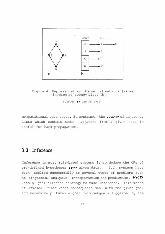
Figure 4. Representation of a neural network (a) asinverse adjacency lists (b) .

Source: Fu and Fu 1990

computational advantages. By contrast, the schene of adjacency

lists which contain nodes adjacent from a given node is

useful for back-propagation.

3.3 Inference

Inference in most rule-based systems is to deduce the CFs of

pre-defined hypotheses from given data. Such systems have

been applied successfully to several types of problems such

as diagnosis, analysis, interpretation and prediction. MYCIN

uses a goal-oriented strategy to make inference. This means

it invokes rules whose consequents deal with the given goal

and recursively turns a goal into subgoals suggested by the

63

antecedents of rules. By contrast, a system which adopts a

data-driven strategy will select rules whose antecedents are

matched by the database. Despira the difference between the

rule selection between these two strategies, inference in

rule-based system is a process cf propagating and combining

CFs through the belief network. Since inference in the

neural network involves a similar process, with CFs replaced

by activation levels, the formulae for computing CFs can be

applied to compute the activaticr. level at each concept node

in the conceptualization.

If a rule-based system involves circularity (cyclic

reasoning), then inference in zs.e neural networks mapped by

such a system is characterized by not only propagation and

combination of activations but also iterative search for a

stable state, if it converges, in an extremely short period

of time measured at the unit si the time constant of the

neural circuit.

The inference capability of "he neural network is derived

from the collective behavicr of simple computational

mechanisms at individual nodes. The output of a node is a

function of the weighted sum of its inputs. In a biological

neuron, if and only if its input exceeds a certain threshold,

the neuron will fire. For an artificial neuron, continuous

non-linear transfer functions such as the sigmoid function

and non-continuous ones such as threshold logic have been

defined. A neural network is often arranged as

single-layered or multi-layers::, and is organized as

feedforward or with collateral or recurrent circuits.

Different architectures are taken in accordance with the

problem characteristics.

In a feedforward neural network as discussed in the

previous chapter the inference bahavior is characterized by

64

propagating and combining activations successively in the

forward direction from input to output layers. Collateral

inhibition and feedback mechanisms are implemented using

collateral and recurrent circuits, respectively. They are

employed for various purposes. For instance, the

winner-take-all strategy can be implemented with collateral

inhibition circuits. Feedback mechanisms are important in

adaptation to the environment. As to the layered arrangement,

multi-layered neural networks are more advantageous than

single-layered networks in performing non-linear

classification. This advantage ster.s from the non-linear

operation at the hidden nodes. For instance, exclusive-OR

can be simulated by a bi-layered neural network but not by

any single-layered one. The principle of maximum information

preservation (informax principle) has been proposed for

information transformation from one layer to another in a

neural network [Linsker 1988]. This principle can shed light

on the design of a neural network for information processing.

The inference tasks performed by the neural network

generally fall into four categories: pattern recognition,

association, optimization and self-organization. A

single-layered network can act as a linear discriminant,

whereas a multi-layered network can be an arbitrary non-

linear discriminant. Association performed by the neural

network is content-directed allowing incomplete matching.

Optimization problems can be solved by implementing cost

function as neural circuits and optimizing them.

Self-organization is the way the neural network evolves

unsupervisedly in response to environmental changes.

Clustering algorithms can be implemented by neural networks

with self-organization abilities. (See previous chapter for

details) .

65

MYCIN like expert systems will be mapped into neural

networks which are in general feedforward and multi- layered,

and perform tasks close to pattern recognition. By

capitalizing on all inference capabilities of neural

networks, it is possible to develop expert systems more

versatile than the existing ones.

3.4 Learning

Learning in the conceptualization is the process of modifying

connection weights to achieve correct inference behavior. The

following will show how to apply the back-propagation rule to

learn and how to revise rules and/or data on the basis of the

results through learning.

In a knowledge-based system, the issue of learning deals

with acquiring new knowledge and maintaining integrity of

the knowledge base. The knowledge base is constructed

through a process called knowledge engineering (encoding of

expert knowledge) or through machine learning.

When errors are observed in the conclusions made by a

rule-based system, an issue is raised of how to identify and

correct the rules or data responsible for these errors. The

problem of identifying the sources of errors is known as the

blame assignment problem.

Previous approaches [Poitakis 1982; Suwa et al. 1984;

Wilkins and Buchanan 1986] only focus on how to revise a

rule-based system. Among these TEIRESIAS [Davis 1976] is a

typical work. It maintains the integrity of knowledge base

by interacting with experts. However, as the size of the

knowledge base grows, it is no longer feasible for human

66

experts to consider all possible interactions among knowledge

in a coherent and consistent way. TMS [Doyle 1979] resolves

inconsistency by altering a minimal set of beliefs, but it

lacks the notion of uncertainty in the method itself.

Symbolic machine learning techniques such as the RL program

[Fu 1985] can learn and debug knowledge but in general do not

address the case when the knowledge involves intermediate

concepts which are not used to describe the training samples.

TEIRESIAS may be confronted with the following problems.

First, incorrect conclusions may be due to data errors.

Second experts know the strengths of inference for each

individual rule, but it may be difficult for them to

determine the rule strengths in such a way that dependencies

among rules are carefully considered to meet the system

assumptions. For instance, in MYCIN, since certainty factors

are combined under the assumption of independence, the

certainty factors assigned to two dependent rules should be

properly adjusted so as to meet this assumption.

3.4.1 Back Propagation of Error

An error refers to the disagreement between the belief values

generated by the system and that indicated by a knowledge

source assumed to be correct (eg., an expert) with respect to

some fact. The back propagation rule developed in the neural

network approach [Rumelhart et.al 1986] is a recursive

heuristic which propagates backwards errors at a rule to all

nodes pointing to that node, and modifies the weights of

connections heading into nodes with errors. First we will

restrict our attention to single-layered networks involving

only input and output neurons.

In each inference task, the system arrives at the belief

values of final hypotheses given those of input data. The

67

belief values of input data form an input pattern (or an

input vector) and those of final hypotheses form an output

pattern (or an output vector) Sy"stem error refers to the case

when incorrect output patterns are generated by the system.

When the system error arises, we use the instance consisting

of the input pattern given for inference and the correct

output pattern to train the network. The instance is

repeatedly used to train the network until a satisfactory

performance is reached. Since the network may be incorrectly

trained by that instance, we also maintain a set of reference

instances to monitor the learning process. This reference set

is consistent with the knowledge base. If, during learning,

some instances in the reference instances set becone

inconsistent, they will be added to the learning process.

On a given trial, the network generates an output vector

given the vector of the training instance. The discrepancy

obtained by. subtracting the network's vector from the

desired output vector serves as the basis for adjusting the

strengths of the connections involved. The back-propagation

rule adapted from [Rumelhart et.al (1986) is formulated as

follows.

AWj: = rDj(dOj /dWjj) (1)

where Dj = Tj - Oj, AWj; is the weight (strength) adjustment of

the connection from input node i to the output node j, r is a

trial independent learning rate, Dj# is the discrepancy between

the desired belief value (T.) and the network's belief value

(Oj) at node j, and the term do, /dlty is the derivative of Oj

with respect to Wjj. According to this rule the magnitude of

weight adjustment is proportional to the product of the

discrepancy and the derivative above.

68

The back-propagation rule is applicable to belief

networks where the propagation and the combination of belief

values are determined by differentiable mathematical

functions. As shown in equation (1), the mathematical

requirement for applying the back-propagation rule is that

the relation between the output activation (0,) and the input

weight (Wjj) is determined by a differentiable function. In

belief networks, this relation is differentiable if the

propagation and the combination functions are differentiabla.

Since combining belief values in most rule-based systems

involves such logic operations as conjunction or disjunction,

the back-propa-gation rule is applied after turning the

conjunction operator into multiplication and the disjunction

operator into summation.

A multi-layered network [Jones and Hoskins 1987] involves

at least three levels; one level of input nodes one level of

output nodes and one or more levels of middle nodes.

Learning in a multi-layered network is more difficult because

the behavior of the middle nodes is not directly observable.

Modifying the strengths of the connections pointing to a

middle node entails the knowledge of the discrepancy between

the network's value and the desired belief value at the

middle node. The discrepancy at a middle node can be

derived from the discrepancies at output nodes which receive

activations from the middle node. It can be shown that the

discrepancy at middle node j is defined by

where Dk is the discrepancy at node k, In the summation,

each discrepancy Dk is weighted by the strength of the

connection pointing from middle node j to node k. This is a

recursive definition in which the discrepancy at a middle

69

node is always derived from discrepancies at nodes at the

next higher level.

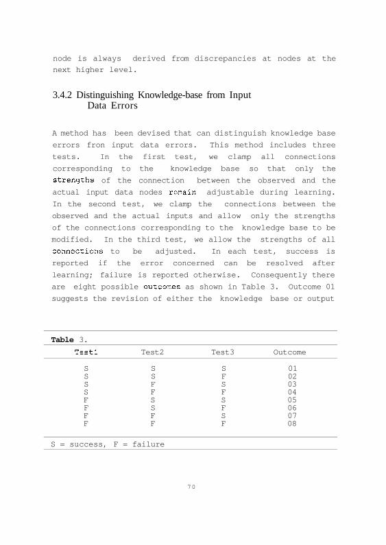
3.4.2 Distinguishing Knowledge-base from InputData Errors

A method has been devised that can distinguish knowledge base

errors fron input data errors. This method includes three

tests. In the first test, we clamp all connections

corresponding to the knowledge base so that only the

strengths of the connection between the observed and the

actual input data nodes remain adjustable during learning.

In the second test, we clamp the connections between the

observed and the actual inputs and allow only the strengths

of the connections corresponding to the knowledge base to be

modified. In the third test, we allow the strengths of all

connections to be adjusted. In each test, success is

reported if the error concerned can be resolved after

learning; failure is reported otherwise. Consequently there

are eight possible outcomes as shown in Table 3. Outcome 01

suggests the revision of either the knowledge base or output

70

Table 3.

Testl Test2 Test3 Outcome

S S S 01S S F 02S F S 03S F F 04F S S 05F S F 06F F S 07F F F 08

S = success, F = failure

data. In this case, an expert's opinion is needed to decide,

which should be revised. Outcome 02 is ignored. Outcone 03

suggests the revision of output data. Outcome 04 is unlikely

and is ignored. Outcome 05 suggests the revision of the

knowledge base. Outcome 06 is also unlikely and is ignored.

Outcome 07 suggests the revision of both the knowledge base

and data. Outcome 08 is a deadlock which demands an expert

to resolve.

3.4.3 Revision Operations

The revision of the above tests will indicate whether the

knowledge base or input data(or both) should be revised. The

strengths of the connections in the network (representing the

knowledge base and input data) have been revised after

learning. The next question is how to revise the knowledge

base and/or input data according to the revisions made in the

network. The revision of the knowledge base will be dealt

with first.

Basically, there are five operators for rule revision

• modification of strengths

• deletion

• generalization,

• specialization, and

• creation

However not all the five operators are suitable in the

neural network approach to editing rules. Each operator is

examined below.

The modification of operator strengths is straight-

forward since the strength of a rule is just a copy of the

weight of the corresponding connection and the weights of

71

connections have been modified after learning with the

back-propagation rule. If the weight change is trivial, we

just keep the rule strength before learning.

The deletion operator is justified by Theorem l.

Theorem l: In a rule-based system if the following conditions

are met:

1. the belief value of the conclusion is determined by

the product of the belief value of the premise ar.d

the rule strength.

2. the absolute value of any belief value and the rule

strength is not greater than 1, and

3. any belief value is rounded off to zero if its

absolute value is below threshold k (k is a real

number between 0 and 1).

then the deletion of rules with strengths below k will not

affect the belief values of the conclusions arrived at by the

system.

Proof: Frcr. condition 1 and 2 if the strength of rule R is

below k, the belief value of its conclusions is always below

k. From condition 3, the belief value of the conclusion

made by rule R will always be rounded off to zero. Since

rule R is not effective in making any conclusion, it can be

deleted. Thus the deletion of such rules as rule R will not

affect the system conclusions.

Accordingly deletion of rule is indicated when its

absolute strength is below the predetermined threshold. In

MYCIN-like system, the threshold is 0.2

72

The deletion operator is also justified by the following

argument. Suppose we add some connections to a neural network

that has already reached an equilibrium and assign weights to

these added connections in such a way that incorrect output

vectors are generated. Thus, these conditions are

semantically inconsistent. Then, if we train the network

with correct samples, the weights of the added connections

will be modified in the direction of minimizing their effect.

What happens is that the weights will go towards zero and

even cross zero during training. In practice, we set a

threshold so that when the shift towards zero for a

connection weight is greater than this threshold, we delete

the connection.

Generalization of a rule can be done by removing scne

conditions from its premise, whereas specialization can be

done by adding more conditions to the premise. If the

desired belief value of a conclusion is always higher than

that generated by the network and the discrepancy resists

decline during learning, it is suggested that rules

supporting these conclusions be generalized. Or on the other

hand, if the discrepancy is negative and resistant,

specialization of a rule may involve qualitative changes of

nodes. The back propagation rule has not yet been powerful

enough to make this kind of change except deletion of

conditions for generalization.

Creation of new rule involves establishment of new

connections. Whereas we delete a rule if its absolute

strength is below a threshold, we may establish a new

connection when its absolute strength is above the threshold.

To create new rules we need to create some additional

connections which have the potential to become rules.

Without any bias, one may need an inference network where all

data are fully connected to all intermediate hypotheses,

73

which in turn are fully connected to all final hypotheses.

This is not a feasible approach unless the system is small.

From the above analyses, we allow only the modification

of strengths and deletion operators in the neural network

approach to rule revision.

Revision of input data is much simpler. If the weight of

the connection between an observed and an actual input node

after learning is below a predeternined threshold, or the

shift towards zero is above a certain value, the

corresponding input data attribute is treated as false and

deleted accordingly.

It has been known that noise associated with training

instances will affect the quality of learning. In the neural

network approach, since noise will be distributed over the

network, its effect on individual connections is relatively

minor. In practice, perfect training instances are neither

feasible nor necessary. As long as most instances are

correct, a satisfactory performance can be achieved.

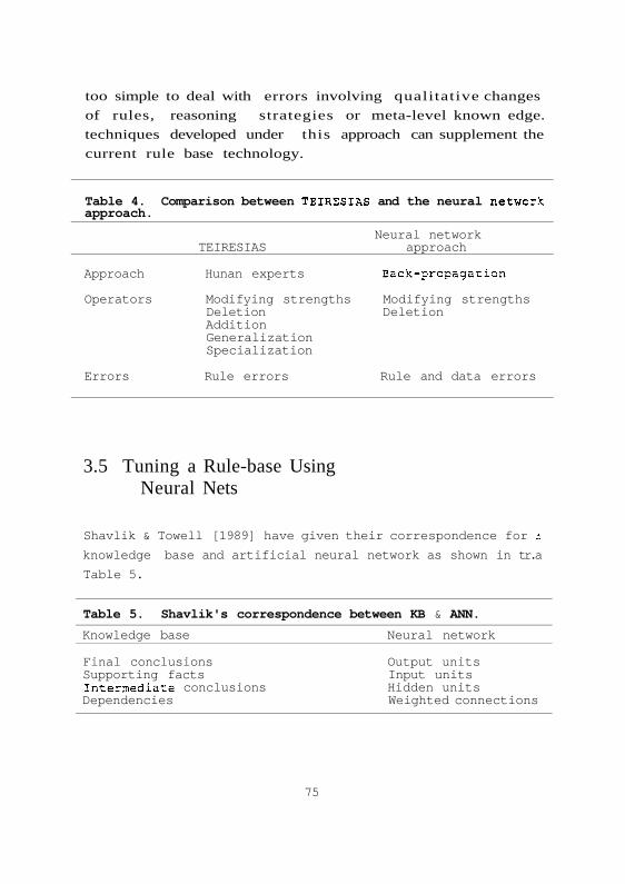
The comparison between the TEIRESIAS approach and the

neural network approach to error handling is shown in table

4. The neural network approach may be more useful than

TEIRESIAS in handling multiple errors or errors involving

some unobservable concepts which human experts may have

difficulties in dealing with. In addition, the back

propagation rule can be uniformly applied to the whole rule

base, whereas human experts may focus on certain parts of the

rule base consciously or subconsciously. Also Wilkins and

Buchanan [1986], suggested that the only proper way to cope

with deleterious interactions among rules is to delete

offending rules. In light of this view the deletion operator

is very useful. While the neural network approach is still

74

too simple to deal with errors involving qualitative changes

of rules, reasoning strategies or meta-level known edge.

techniques developed under this approach can supplement the

current rule base technology.

3.5 Tuning a Rule-base UsingNeural Nets

Shavlik & Towell [1989] have given their correspondence for a

knowledge base and artificial neural network as shown in tr.a

Table 5.

75

Table 4. Comparison between TEIRESIAS and the neural networkapproach.

Neural networkTEIRESIAS approach

Approach Hunan experts Back-propagation

Operators Modifying strengths Modifying strengthsDeletion DeletionAdditionGeneralizationSpecialization

Errors Rule errors Rule and data errors

Table 5. Shavlik's correspondence between KB & ANN.

Knowledge base Neural network

Final conclusions Output unitsSupporting facts Input unitsIntermediate conclusions Hidden unitsDependencies Weighted connections

Knowledge based artificial neural network (KBANN) uses a

knowledge base (KB) of domain specific inference rules in the

form of PROLOG-like clauses to define what is initially known

about a topic. The KB need be neither complete nor correct,

but needs to only support approximately correct explanations.

KBANN translates the KB into an artificial neural network

(ANN) in which units and links in the ANN correspond to parts

of the KB as shown in the Table 5.

3.5.1 Translation of Rules

Rules are assumed to be conjuctive, non-recursive and

variable-free; disjuncts are encoded as multiple rules. The

KBANN method sets weights on links and biases of units so

that, units have significant activation only when the

corresponding deduction could be made using the KB. For

example, assume there exists a rule in the KB with n

mandatory antecedents (which must be true) and m prohibitory

antecedents (which are not true). The system sets weights on

links in the ANN corresponding to the mandatory and

prohibitory dependencies of the rule to w and -w

respectively. The bias on the unit corresponding to the

rule's consequent is set to n*w-f, f is chosen such that

units have activation approximately 0.9 when Their

antecedents are satisfied and activation of approximately 0.1

otherwise.

KBANN handles disjuncts by creating units L, and L, which

correspond to R, and R2, using the approach for conjunctive

rules described above. These units will only be active when

their corresponding rule is true. KBANN then connects L, and

In to L by a link of these weight w and sets the bias of L to

w -f. Hence, L will be active when either L, or In. is active.

76

This concept is explained by means of an example by Towelle t . a l [1990].

3.5.2 Overview of the KBANN Algorithm is as

Follows

1. Translate rules to set initial network structure.

2. Add units not specified by translation.

3. Add links not specified by translation.

4. Perturb the network by adding near zero random numbers to

all link weights and biases.

3.5.3 Limitations in Shavlik's Approach

a) They have assumed certainty factors of all premises

(including condition & action part) and rule strengths to

be 1. i.e., they have proposed logical reasoning using

NN.

b) They assumed an output of a neuron to be a binary feature

(either 0 or 1) . But in the real case, when we are

considering uncertainty factors which are not equal to

1, it will not be so. While they just mentioned about

non-binary features but did not elaborate any further.

c) To handle disjunctive rule, a new node has to be inserted

in a NN.

Note: Obviously, non-binary features can be used to

implement plausible reasoning.

77

3.6 Inducing Rules for aConnectionist ES

Gallant has implemented a two-program package for constructing

connectionist expert systems from training examples. The

first program is a network knowledge base generator that uses

several connectionist learning techniques, and the second

(MACIE) is a stand alone expert system inference engine that

interprets such knowledge bases. [Gallant 1988]

3.6.1 Network Properties

A connectionist model consists of a network of (more or less)

autonomous processing units called cells that are joined by

directed arcs. Each arc ("connection") has a numerical

weight Wjj that roughly corresponds to the influence of cell

Uj on cell u,. Positive weights indicate reinforcement;

negative weights represent inhibition. The weights determine

the behavior of the network, playing some what the same role

as a conventional program. They classified networks as

either feed forward networks if they do not contain directed

cycles or feed-back networks if they do contain such cycles.

Every cell Uj (except for input cells) computes its new

activation u, as a function for the weighted sum of the inputs

to cell u, from directly connected cells.

nSj = E WyUj for j = 0 to j = n

u, = f(S,)

If Uj is not connected to Uj, then Wy = 0 . By convention there

is a cell u0 whose output is always +1 that is connected to

every cell U; (except for input cells). The corresponding

weights (Wi0) are called biases.

78

They have given a sample problem for diagnosis and

treatment of acute Sachrophagal disease [Buchanan and

Shortliffe 1985] .

To generate the connectionist knowledge base, they have

used following specifications:

• Name of each cell corresponding to variable of

interest (symptoms, diseases, treatments). Each

variable will correspond to a cell u(.

• A question for each input variable, to elicit the

value of that variable from the user.

• Dependency information for intermediate variables

(diseases) and output variables (treatments). Each

of these variables has a list of other variables

whose values suffice for computing it.

• The final information supplied to the learning problem

is the set of training examples.

They have developed a procedure called pocket algorithm

that generates weights for discrete networks. Training

algorithm specifies the desired activations for intermediate

and output cells in the network(easy learning).

k

W*: for cell u let {Ek} be the set of training example

activations.

k

{Ck} be the corresponding correct activations for u.

Pocket algorithm is a modified perceptron algorithm. It

computes perceptron weight vectors, P, which occasionally

replace pocket weight vectors w*.

79

They have defined rule as an example Er with ther

corresponding classification cr that must be satisfied by

the resulting w* Gallant has named his inference engine as

MACIE - Matrix Controlled inference engine. It is

represented internally by weight matrix.

3.6.2 ES Algorithms

Initial information — the program starts by listing for the

user all variables and allowing any input variable to

be initialized to true or false.

Inference/forward chaining: It is usually possible to deduce

the activation for cell u, without knowing the values of all

of its inputs.

Addition of a new rule: Directly contradiction values Er = E1

but Cr <> Cs are not allowed.

3.6.3 Limitations in Gallant's Approach

a) MACIE is an impossible model for reasoning.

b) Gallant worked with discrete connectionist models.

There are many incomplete areas left in this work.

3.7 Present Work

If is by now quite apparent from the combination of

limitations of the earlier three approaches that they have

80

major drawbacks as discussed earlier and the following

enhancements would be very effective and useful:

a) Combination and propagation of non-binary belief values

in neural networks (rule wise).

b) Evidential reasoning in a network (rule wise).

c) Learning/Training: Process of training the belief values

such that net reaches final conclusion with desired

result.

d) Consistency: Defining the consistency of the rule base in

the connectionist expert system.

e) Learning a new rule: The process of learning new rules

without any major changes to the previous neural net

states, etc.

In the next Chapter we will discuss about how we have

made some of the enhancements mentioned above.

81