Chapter 3 campo de la tierra magnetico

Chapter 3

The Magnetic Field of the Earth

Introduction

Studies of the geomagnetic field have a long history, in particular because of its importance fornavigation. The geomagnetic field and its variations over time are our most direct ways to studythe dynamics of the core. The variations with time of the geomagnetic field, the secular variations,are the basis for the science of paleomagnetism, and several major discoveries in the late fiftiesgave important new impulses to the concept of plate tectonics. Magnetism also plays a major rolein exploration geophysics in the search for ore deposits.Because of its use as a navigation tool, the study of the magnetic field has a very long history, andprobably goes back to the 12

��C when it was first exploited by the Chinese. It was not until 1600

that Gilbert postulated that the Earth is, in fact, a gigantic magnet. The origin of the Earth’s fieldhas, however, remained enigmatic for another 300 years after Gilbert’s manifesto ’De Magnete’.It was also known early on that the field was not constant in time, and the secular variation is wellrecorded so that a very useful historical record of the variations in strength and, in particular, indirection is available for research. The first (known) map of declination was published by Halley(yes, the one of the comet) in 1701 (the ’chart of the lines of equal magnetic variation’, also knownas the ’Tabula Nautica’).The source of the main field and the cause of the secular variation remained a mystery sincethe rapid fluctuations seemed to be at odds with the rigidity of the Earth, and until early thiscentury an external origin of the field was seriously considered. In a breakthrough (1838) Gausswas able to prove that almost the entire field has to be of internal origin. Gauss used sphericalharmonics and showed that the coefficients of the field expansion, which he determined by fittingthe surface harmonics to the available magnetic data at that time (a small number of magnetic fieldmeasurements at intervals of about 30 � along several parallels - lines of constant latitude), werealmost identical to the coefficients for a field due to a magnetized sphere or to a dipole. In fact,he also showed from a spectral analysis that the best fit to the observed field was obtained if thedipole was not purely axial but made an angle of about 11 � with the Earth’s rotation axis.An outstanding issue remained: what causes the internal field? It was clear that the temperatures inthe interior of the Earth are probably much too high to sustain permanent magnetization. A majorleap in the understanding of the origin of the field came in the first decade of this century whenOldham (1906) and Gutenberg (1912) demonstrated the existence of a (outer) core with a very lowviscosity since it did not seem to allow shear wave propagation ( � rigidity � =0). So the rigidityproblem was solved. From the cosmic abundance of metallic iron it was inferred that metallic iron

67

68 CHAPTER 3. THE MAGNETIC FIELD OF THE EARTH

could be the major constituent of the (outer) core (the seismologist Inge Lehman discovered theexistence of the inner core in 1936). In the 40-ies Larmor postulated that the magnetic field (andits temporal variations) were, in fact, due to the rapid motion of highly conductive metallic ironin the liquid outer core. Fine; but there was still the apparent contradiction that the magnetic fieldwould diffuse away rather quickly due to ohmic dissipation while it was known that very old rocksrevealed a remnant magnetic field. In other words, the field has to be sustained by some, at thattime, unknown process. This lead to the idea of the geodynamo (Sir Bullard, 40-ies and 50-ies),which forms the basis for our current understanding of the origin of the geomagnetic field. Thetheory of magneto-hydrodynamics that deals with magnetic fields in moving liquids is difficultand many approximations and assumptions have to be used to find any meaningful solutions. Inthe past decades, with the development of powerful computers, rapid progress has been made inunderstanding the field and the cause of the secular variation. We will see, however, that there arestill many outstanding questions.

Differences and similarities with Gravity

Similarities are:

� The magnetic and gravity fields are both potential fields, the fields are the gradient of somepotential

�, and Laplace’s and Poisson’s equations apply.

� For the description and analysis of these fields, spherical harmonics is the most convenienttool, which will be used to illustrate important properties of the geomagnetic field.

� In both cases we will use a reference field to reduce the observations of the field.

� Both fields are dominated by a simple geometry, but the higher degree components arerequired to get a complete picture of the field. In gravity, the major component of the fieldis that of a point mass M in the center of the Earth; in geomagnetism, we will see that thefield is dominated by that of an axial dipole in the center of the Earth and aligned along therotational axis.

Differences are:

� In gravity the attracting mass � is positive; there is no such thing as negative mass. Inmagnetism, there are positive and negative poles.

Figure 3.1:

3.1. THE MAIN FIELD 69

� In gravity, every mass element��

acts as a monopole; in contrast, in magnetism isolatedsources and sinks of the magnetic field � don’t exist ( �� ) and one must alwaysconsider a pair of opposite poles. Opposite poles attract and like poles repel each other. Ifthe distance

�between the poles is (infinitesimally) small � dipole.

� Gravitational potential (or any potential due to a monopole) falls of as 1 over � , and thegravitational attraction as 1 over �� . In contrast, the potential due to a dipole falls of as 1over �� and the field of a dipole as 1 over �� . This follows directly from analysis of thespherical harmonic expansion of the potential and the assumption that magnetic monopoles,if they exist at all, are not relevant for geomagnetism (so that the �� component is zero).

� The direction and the strength of the magnetic field varies with time due to external andinternal processes. As a result, the reference field has to be determined at regular intervalsof time (and not only when better measurements become available as is the case with theInternational Gravity Field).

� The variation of the field with time is documented, i.e. there is a historic record available tous. Rocks have a ’memory’ of the magnetic field through a process known as magnetization.The then current magnetic field is ’frozen’ in a rock if the rock sample cools (for instance,after eruption) beneath the so called Curie temperature, which is different for differentminerals, but about 500-600 � C for the most important minerals such as magnetite. This isthe basis for paleomagnetism. (There is no such thing as paleogravity!)

3.1 The main field

From the measurement of the magnetic field it became clear that the field has both internal andexternal sources, both of which exhibit a time dependence. Spherical harmonics is a very conve-nient tool to account for both components. Let’s consider the general expression of the magneticpotential as the superposition of Legendre polynomials:

�� "! #$ % &('%$� &*) +-,/.0�1 %32 '(4 5 �%7698�:

�;�=<?> �%@:�ACB �;�ED, 0. 1 % 4 5�F �% 698�: �;�=<?> F �% :�AGB �;�EDIH�J �% � 698�: �K�/� (3.1)

or, assuming Einstein’s summation convention (implicit summation over repeated indices), wecan write:

�L�� ! +(M �%ON !��P%Q2 ' <SR �%TN �!EP

%H�J �% � 698�: �� (3.2)

where

M �%and R �% are the amplitude factors of the contributions of the internal and external

sources, respectively. (Note that, in contrast to the gravitational potential, the first degree is ��VU ,since �� would represent a monopole, which is not relevant to geomagnetism.)


Intermezzo 3.1 UNITS OF CONFUSION

The units that are typically used for the different variables in geomagnetism are somewhat confusing, andup to 5 different systems are used. We will mainly use the Systeme International d’Unites (S.I.) and mentionthe electromagnetic units (e.m.u.) in passing. When one talks about the geomagnetic field one often talksabout

�, measured in T (Tesla) (= kg �

�s ��) or nT (nanoTesla) in S.I., or Gauss in e.m.u. In fact,

�is the

magnetic induction due to the magnetic field � , which is measured in Am ��

in S.I. or Oersted in e.m.u.For the conversions from the one to the other unit system: T = 10

�G(auss) � 1nT = 10 �

�G = 1 � (gamma).�

= �� with the magnetic permeability in free space; = 4 �� 10 ��

kgmA ��

[=NA ��

= H(enry)m �

�], in S.I., and = 1 G Oe in e.m.u. So, in e.m.u.,

�= � , hence the liberal use of

�for the Earth’s

field. The magnetic permeability is a measure of the “ease” with which the field � can penetrate into amaterial. This is a material property, and we will get back to this when we discuss rock magnetism.In the next table, some of the quantities are summarized together with their units and dimensions. Thereare only 4 so-called dimensions we need. These are (with their symbol and standard units) mass [ � (kg)],length [ � (m)], time [ � (s)] and current [ � (Ampere)].

Quantity Symbol Dimension S.I. Unitsforce � MLT �

�Newton (N)

charge � IT Coulomb (C)electric field � MLT �

�I ��

N/Celectric flux �� ML

�T �

�I ��

N/C m�

electric potential � � ML�T �

�I ��

Volt (V)magnetic induction

�MT �

�I ��

Tesla (T)magnetic flux �� ML

�T �

�I ��

Weber (Wb)magnetic potential �� MLT �

�I ��

T mpermittivity of vacuum M �

�L �

�T�I�

C�/(N m

�)

permeability of vacuum MLT ��I ��

Wb/(A m)resistance ! ML

�T �

�I ��

Ohm ( " )resistivity # ML

�T �

�I ��

" m

3.2 The internal field

The internal field has two components: [1] the crustal field and [2] the core field.

The crustal field

The spatial attenuation of the field as 1 over distance cubed means that the short wavelength vari-ations at the Earth’s surface must have a shallow source. Can not be much deeper than mid crust,since otherwise temperatures are too high. More is known about the crustal field than about thecore field since we know more about the composition and physical parameters such as temperatureand pressure and about the types of magnetization. Two important types of magnetization:

� Remanent magnetization (there is a field $ even in absence of an ambient field). If thispersists over time scales of % � U '&�� years, we call this permanent magnetization. Rockscan acquire permanent magnetization when they cool beneath the Curie temperature (about500-600 � for most relevant minerals). The ambient field then gets frozen in, which is veryuseful for paleomagnetism.

3.2. THE INTERNAL FIELD 71

� Induced magnetization (no field, unless induced by ambient field).

No mantle field

Why not in the mantle? Firstly, the mantle consists mainly of silicates and the average conductivityis very low. Secondly, as we will see later, fields in a low conductivity medium decay very rapidlyunless sustained by rapid motion, but convection in the mantle is too slow for that. Thirdly, per-manent magnetization is out of the question since mantle temperatures are too high (higher thanthe Curie temperature in most of the mantle).

The core field

The temperatures are too high for permanent magnetization. The field is caused by rapid (andcomplex) electric currents in the liquid outer core, which consists mainly of metallic iron. Con-vection in the core is much more vigorous than in the mantle: about 10

�times faster than mantle

convection (i.e, of the order of about 10 km/yr).Outstanding problems are:

1. the energy source for the rapid flow. A contribution of radioactive decay of Potassium and,in particular, Uranium, can - at this stage - not be ruled out. However, there seems to beincreasing consensus that the primary candidate for the provision of the driving energy isgravitational energy released by downwelling of heavy material in a compositional convec-tion caused by differentiation of the inner core. Solidification of the inner core is selec-tive: it takes out the iron and leaves behind in the outer core a relatively light residue thatis gravitationally unstable. Upon solidification there is also latent heat release, which helpsmaintaining an adiabatic temperature gradient across the outer core but does not effectivelycouple to convective flow. The lateral variations in temperature in the outer core are proba-bly very small and the role of thermal convection is negligible. Any aspherical variations indensity would be annihilated quickly by convection as a result of the low viscosity.

2. the details of the pattern of flow. This is a major focus in studies of the geodynamo.

The knowledge about flow in the outer core is also restricted by observational limitations.

� the spatial attenuation is large since the field falls of as 1 over �� . As a consequence effectsof turbulent flow in the core are not observed at the surface. Conversely, the downwardcontinuation of small scale features in the field will be hampered by the amplification ofuncertainties and of the crustal field.

� the mantle has a small but non-zero conductivity, so that rapid variations in the core fieldwill be attenuated. In general, only features of length scales larger than about 1500 km( ��IU��K� U�� ) and on time scales longer than 1 to 5 year are attributed to core flow, althoughthis rule of thumb is ad hoc.

The core field has the following characteristics:

1. 90% of the field at the Earth’s surface can be described by a dipole inclined at about 11 �to the Earth’s spin axis. The axis of the dipole intersects the Earth’s surface at the so-called geomagnetic poles at about (78.5 � N, 70 � W) (West Greenland) and (75.5 � S, 110 � E).


In theory the angle between the magnetic field lines and the Earth’s surface is 90 � at thepoles but owing to local magnetic anomalies in the crust this is not necessarily the case inreal life.

The dipole field is represented by the degree 1 ( � � U ) terms in the harmonic expansion.From the spherical harmonic expansion one can see immediately that the potential due toa dipole attenuates as 1 over �� . For � � U the three possible coefficients are

� 5 )' � 5 '' ��> '' �and they represent one axial (

5 )' ) and two equatorial components of the field. (with5 '' taken

along the Greenwich meridian). At any point� �� outside the source of the field, i.e,

outside the core, the dipole field can be composed as the sum of these three components.

Figure 3.2:

2. The remaining 10% is known as the non-dipole field and consists of a quadrupole ( � �� ), and octopole ( � � � ), etc. We will see that at the core-mantle-boundary the relativecontribution of these higher degree components is much larger!

Note that the relative contribution 90% � 10% can change over time as part of the secularvariation.

3. The strength of the Earth’s magnetic field varies from about 60,000 nT at the magnetic poleto about 25,000 nT at the magnetic equator. (1nT = 1 � = 10 �

'Wb m � ).

4. Secular variation: important are the westward drift and changes in the strength of the dipolefield.

5. The field may or may not be completely independent from the mantle. Core-mantle couplingis suggested by several observations (i.e., changes of the length of day, not discussed here)and by the suggested preferential reversal paths.

3.3 The external field

The strength of the field due to external sources is much weaker than that of the internal sources.Moreover, the typical time scale for changes of the intensity of the external field is much shorterthan that of the field due to the internal source. Variations in magnetic field due to an external origin(atmospheric, solar wind) are often on much shorter time scales so that they can be separated fromthe contributions of the internal sources.

3.4. THE MAGNETIC INDUCTION DUE TO A MAGNETIC DIPOLE 73

The separation is ad hoc but seems to work fine. The rapid variation of the external field can beused to study the (lateral variation in) conductivity in the Earth’s mantle, in particular to depthof less than about 1000 km. Owing to the spatial attenuation of the coefficients related to theexternal field and, in particular, to the fact that the rapid fluctuations can only penetrate to a certaindepth (the skin depth, which is inversely proportional to the frequency), it is difficult to study theconductivity in the deeper part of the lower mantle.

3.4 The magnetic induction due to a magnetic dipole

Magnetic fields are fairly similar to electric fields, and in the derivation of the magnetic inductiondue to a magnetic dipole, we can draw important conclusions based on analogies with the electricpotential due to an electric dipole. We will therefore start with a brief discussion of electric dipoles.On the other hand, our familiarity with the gravity field should enable us to deduce differences andsimilarities of the magnetic field and the gravity field as well. In this manner, we will start with thefield due to a magnetic dipole — the simplest configuration in magnetics — in a straightforwardanalysis based on experiments, and subsequently extend this to the field induced by higher-order“poles”: quadrupoles, octopoles, and so on. The equivalence with gravitational potential theorywill follow from the fact that both the gravitational and the magnetic potential are solutions toLaplace’s equation.

The electric field due to an electric dipole

The law obeyed by the force of interaction of point charges � (in vacuum) was established experi-mentally in 1785 by Charles de Coulomb. Coulomb’s Law can be expressed as:

� �� ) �� U�� ) � ) �� (3.3)

where�� is the unit vector on the axis connecting both charges. This equation is completely anal-

ogous with the gravitational attraction between two masses, as we have seen. Just as we definedthe gravity field to be the gravitational force normalized by the test mass, the electric field � isdefined as the ratio of the electrostatic force to the test charge:

� � �� ) � (3.4)

or, to be precise,

� �� A �� ) �� ) � (3.5)

Now imagine two like charges of opposite sign <�� and �� , separated by a distance�, as in Figure

3.3. At a point J in the equatorial plane, the electrical fields induced by both charges are equalin magnitude. The resulting field is antiparallel with vector � . If we associate a dipole momentvector � with this configuration, pointing from the negative to the positive charge and whereby� � � �� , the field strength at the equatorial point J is given by:R �� U�� ) � � �� (3.6)


Figure 3.3:

Next, consider an arbitrary point J at distance � from a finite dipole with moment � . In gravitywe saw that the gravitational field (the gravitational force per unit mass), led to the gravitationalpotential at point J due to a mass element

��given by

�� '. We can use this

as an analog for the derivation of the potential due to a magnetic dipole, approximated by a set ofimaginary monopoles with strength � . To get an expression for the magnetic potential we have toaccount for the potential due to the negative ( � � ) and the positive ( < � ) pole separately.With � some constant we can write

�L� � � N U� 2 � U� � P � � � '0 � � '0�� (3.7)

and for small� U� N U� 2 � U� � P �� N U� P (3.8)

eq. (3.7) becomes:

� � � � � �� N U� P (3.9)

�� U�� is the directional derivative of U�� in the direction of�. This expression can be written as

the directional derivative in the direction of � by projecting the variations in the direction of � on� (i.e., taking the dot product between � or � and � ):�� N U� P � �� N U� P 698�: � � � U� 698�: � (3.10)

Since�� U�� this expression means that the potential due to a dipole is the directional

derivative of the potential due to a monopole. (Note that � is the angle between the dipole axis �and � J (or � ) and thus represents the magnetic co-latitude.)Just as the Newtonian potential was proportional to �� , the constant � must be proportional tothe strength of the poles, or to the magnitude of the magnetic moment � � � � � � � � � � � �� . We have, in S.I. units,

� � � � ) �

698�: �� ) �-� �� )� � � �� (3.11)

3.5. MAGNETIC POTENTIAL DUE TO MORE COMPLEX CONFIGURATIONS 75

Intermezzo 3.2 MAGNETIC FIELD INDUCED BY ELECTRICAL CURRENT

There is no such thing as a magnetic “charge” or “mass” or “monopole” that would make a magnetic forcea law similar to the law of gravitational or electrostatic attraction. Rather, the magnetic induction is bothdefined and measured as the force (called the Lorentz forcea) acting on a test charge �� that travels throughsuch a field with velocity � .

�� (3.12)

On the other hand, it is observed that electrical currents induce a magnetic field, and to describe this, anequation is found which resembles the electric induction to to a dipole. The idea of magnetic dipoles isborn. In 1820, the French physicists Biot and Savart measured the magnetic field induced by an electricalcurrent. Laplace cast their results in the following form:

� � � � � �� (3.13)

An infinitesimal contribution to the magnetic induction� �

due to a line segment

through which flows acurrent

�is given by the cross product of that line segment (taken in the direction of the current flow) and

the unit vector connecting the��

to point

.For a point

on the axis of a closed circular current loop with radius ! , the total induced field

�can be

obtained as:

� � �� !��

� �� (3.14)

In analogy with the electrical field, a dipole moment�

is associated with the current loop. Its magnitudeif given as

� �� ! � � , i.e. the current times the area enclosed by the loop.�

lies on the axis of thecircle and points according in the direction a corkscrew moves when turned in the direction of the current(the way you find the direction of a cross product). Note how similar Eq. 3.14 is to Eq. 3.6: the simplestmagnetic configuration is that of a dipole.The definition of electric or gravitational potential energy is work done per unit charge or mass. In analogyto this, we can define the magnetic potential increment as:� �� ! � (3.15)

What is the potential at a point

due to a current loop? Using Eq. 3.13, we can write Eq. 3.15 as:

� � � � �� #"�� %$ �� & � (3.16)

Working this out (this takes a little bit of math) for a current loop small in diameter with respect to thedistance � to the point

and introducing the magnetic dipole moment

�as done above, we obtain for the

magnetic potential due to a magnetic dipole:

� � � � �� (3.17)

aAfter Hendrik A. Lorentz (1853–1928).

3.5 Magnetic potential due to more complex configurations

Laplace’s equation for the magnetic potential

In gravity, the simplest configuration was the gravity field due to a point mass, or gravitationalmonopole. After that we went on and proved how the gravitational potential obeyed Laplace’s


equation. The solutions were found as spherical harmonic functions, for which the � � termgave us back the gravitational monopole.Magnetic monopoles have not been proven to exist. The simplest geometry therefore is the dipole.If we can prove that the magnetic field obeys Laplace’s equation as well, we will again be ableto obtain spherical harmonic solutions, and this time the � � U term will give us back the dipoleformula of Eq. 3.17.It is easy enough to establish that for a closed surface enclosing a magnetic dipole, just as manyfield lines enter the surface as are leaving. Hence, the total magnetic flux should be zero. Atthe north magnetic pole, your test dipole will be attracted, whereas at the south pole it will berepelled, and vice versa. Remember how this was untrue for the flux of the gravity field: an applefalls toward the Earth regardless if it is at the north, south or any other pole. Mathematicallyspeaking, in contrast to the gravity field, the magnetic field is solenoidal. We can write:

�� " � $ � ��;�� (3.18)

Using Gauss’s law just like we did for gravity, we find that the magnetic induction is divergence-free and with Eq. 3.15 we obtain that indeed� � �� (3.19)

This equation is known in magnetics as Gauss’s Law; we will encounter it again as a specialcase of the Maxwell equations. We have previously solved Eq. 3.19. The solutions are sphericalharmonics, so we know that the solution for an internal field is given by (for �� ! ):

� ��! #$ % &('%$� &*) N ! � P

%32 ' J �% � 698�: �� 4 5 �% 698�: �;� < > � % :�ACB �;�ED � (3.20)

Intermezzo 3.3 SOLENOIDAL, POTENTIAL, IRROTATIONAL

A solenoidal vector field�

is divergence-free, i.e. it satisfies satisfies

� � �� (3.21)

for every vector�

. If this is true, then there exists a vector field such that

�� (3.22)

This follows from the vector identity

� � � � � �� (3.23)

This vector field is a potential field. For a function � satisfying Laplace’s equation �� is solenoidal(and also irrotational). An irrotational vector field � is one for which the curl vanishes:

�� (3.24)


Reduction to the dipole potential

The potential due to a dipole is obtained from Eq. 3.20 by setting ��VU and taking the appropriateassociated Legendre functions:

� � � !K�� 4 5 )' 698�: � < 5 '' 698�: � :�ACB � <?> '' :�ACB � :�AGB � D � (3.25)

This is valid in Earth coordinates, with the � -axis the rotation axis. Earlier, we had obtained Eq.3.17, which we can write, still in geographical coordinates, as:

� � � )� U� � �� < �� < �� (3.26)

Later, we will see how in a special case, we can take the dipole axis to be the � -axis of our coordi-nate system (geomagnetic coordinates or axial dipole assumption). Then, there is no longitudinalvariation of the potential, �� is the only nonzero component and the only coefficient needed is

5 ) ' .Comparing Eqs. 3.25 and 3.26 we see the equivalence of the Gauss coefficients

5 �%and > � % with

the Cartesian components of the magnetic dipole vector:�� !K� 5 ''�� ! � > ''

� � �� !K� 5 )' � (3.27)

Obtaining the magnetic field from the potential

We’ve seen in Eq. 3.15 that the magnetic induction is the gradient of the magnetic potential. It iscertainly more convenient to express the field in spherical coordinates. To this end, we remind thereader of the spherical gradient operator:� � �� < �� U� �� < �� U� :�ACB � �� (3.28)

In other words, the three components of the magnetic induction in terms of the magnetic potentialare given by:

� 0 � �� U� �� U� :�ACB � ��

(3.29)

We remind that�� points in the direction of increasing distance from the origin (outwards from the

Earth),��

in the direction of increasing � (that is, southwards) and�� eastwards. See Figure 3.4.


Figure 3.4:

Geographic and geomagnetic reference frames

It is useful to point out the difference between geocentric (or geographic) and geomagnetic refer-ence frames.In a geomagnetic reference frame, the dipole axis coincides with the � coordinate axis. Since thedipole field is axially symmetric, it is now symmetric around the � -axis. This implies that thereis no longitudinal variation: no � -dependence. The components of the field can be described byzonal spherical harmonics — in the upper hemisphere, field lines are entering the globe, and theyare leaving in the lower hemisphere. Only one Gauss coefficient is necessary:

� )' or � F describethe dipole completely (curled letters used for dipole reference frame). See Figure 3.5(A).In Figure 3.5(B), the dipole is placed at an angle to the coordinate axis. To describe the field,we need more than one spherical harmonic: a zonal and a sectoral one. Longitudinal � -variationis introduced: � �� . We need three Gauss coefficients to describe the dipole behavior:

5 ) ' ,5 '' and > '' . Of course the dipole itself hasn’t changed: its magnitude is now4 � 5 ) ' � < � 5 '' � <� > '' � D�� '�� )' � . Compared to the dipole reference frame, all we have done is a spherical

harmonic rotation, resulting in a redistribution of the magnitude of the dipole over three instead ofone Gauss coefficients.The angle the magnetic induction vector makes with the horizontal is called the inclination

M. The

angle with the geographic North is the declination . In a dipole reference frame, the declinationis indentically zero.Let’s use Eqs. 3.17 and 3.29 to calculate the components of a dipole field in the dipole referenceframe for a few special angles.

� � � )� � � � 698�: �� (3.30)

from which follows that �� 0 � � �� 0 � � 698�: ��

� ) 698�: �� 0 � :�ACB � � � ) :�ACB �� (3.31)

� ) � �� ) � � � �� !�� = 3.03 10 �� T (= 0.303 Gauss) at the surface of the Earth.


Figure 3.5: Geographic and geomagnetic reference frames and how to represent the dipole withspherical harmonics coefficients in both references systems.

So for the magnetic North Pole, Equator and South Pole, respectively, we get the field strengthssummarized in Table 3.1. � � 0 � � ��

North Pole 0 �� ) 0 0

Equator � � 0

� ) 0South Pole 0 � � � ) 0 0

Table 3.1: Field strengths at different latitudesin terms of the field strength at the equator.

So the field at the magnetic equator is half that at the magnetic poles, and at the North Pole itpoints radially inward, but outward at the South Pole.In geomagnetic studies, one often uses

� � � � 0 and � � � �� and R � ��. The magnetic

North Pole is in fact close to the geographic South Pole! The expression for inclination is oftengiven as:

��B M � ��

698�: �:�AGB � � � ��B

�' ��

698� � � � ��

B�� (3.32)


with� �

the magnetic latitude (� � � � � � � ) at which the field line crosses the point � �"! .

Figure 3.6:

3.6 Power spectrum of the magnetic field

The power spectrum

M %at degree � of the field $ is defined as the scalar product $

% � $ % averagedover the surface of the sphere with radius ! . In other words, the definition of

M %is:M % � U� ! �� ) �� ) $

% � $ % ! :�ACB � � � � � � (3.33)

which, with, as we’ve seen $

%equal to

$

% � � �� ! N ! � P%32 ' %$� &*) � 5 �% 698�: �;� < > � % :�ACB �;�� J �% � 698�: �K�� (3.34)

From this, the power spectrum for a particular degree � is given byM % � � �L<�U � %$� &*) 4 � 5 �% � < � > � % � D � (3.35)

The root mean square (r.m.s) field strength at the Earth’s surface for degree � is defined as� % �� M %

and the total r.m.s. field is given by

� � + #$ % &(' M % H �� + #$ % &(' � � <�U � %$� &*) 4 � 5 �% � < � > � % � D H �� (3.36)M %can be plotted as a function of degree � :

The power spectrum consists of two regimes. Up to degree � = 14-15 there is a rapid roll-off of themean square field with degree � . The field is obviously predominated by the lower degree terms,and such a so called “red” spectrum is, of course, consistent with the spherical harmonic expansionfor internal sources, see Eq. 3.20. This part of the spectrum is due to the core field. To be moreprecise, the core field dominates the spectrum up to degree � = 14-15. At higher degrees the corefield is obscured by a flat “white-ish” spectrum where the power no longer seems to depend onthe degree, or, alternatively, the wavelength of the causative anomalies. This part of the spectrummust be due to sources close to the observation points; it relates to the crustal field. We will see

3.7. DOWNWARD CONTINUATION 81

Figure 3.7:

that this field is important even, or, in particular, when one wants to study the magnetic field at thesurface of the outer core, the core mantle boundary (CMB).

3.7 Downward continuation

In order to study core dynamics or the geodynamo one wants to know what the magnetic field isclose to its source, i.e., at the CMB.From Eq. 3.20, we deduce that

�

% � ��

% � ! � N ! � P%32 '

(3.37)

$ � � � �

% � �� $

% � ! � � � <"U � N ! � P%Q2

(3.38)

(3.39)

So for the power spectrum, logically, M % � �� M % � ! � N ! ��P %Q2 �

(3.40)


with

M % � !�� the power at Earth’s surface ( � ��! ).Let’s look at some numbers to illustrate the effect of downward continuation (see Table 3.2).Consider the (r.m.s.) field strength at the equator at both the Earth’s surface ( �@� ! ) and at theCMB ( � �� ! (so that ! � ��VU � � � ) (Use eq. (3.36)).

Surface (nT) CMB (nT)dipole ( � =1) 42,878 258,493quadrupole ( � =2) 8,145 (19% of dipole) 89,367 (35% of dipole)octopole ( � =3) 6,079 (14% of dipole) 121,392 (47% of dipole)

Table 3.2: Field strengths at the surface and the core mantle boundary.

In other words, if the spectrum of the core field is ”red” at the Earth’s surface, it is more ”pink-ish”at the CMB because the higher degree components are preferentially amplified upon downwardcontinuation. However, the amplitude of the higher degree components (the value of the relatedGauss coefficients) is small and, consequently, the relative uncertainty in these coefficients large.Upon downward continuation these uncertainties are — of course — also amplified, so that at theCMB the higher degree components are large but uncertain and the observational constraints forthem are increasingly weak! We can now also understand why the crustal field poses a problem ifone wants to study the core field at the CMB for degrees ��OU � : these high degree componentswill be strongly amplified upon downward continuation and for high harmonic degrees the corefield at the CMB will be contaminated with the crustal field!

3.8 Secular variation

Secular variation is loosely used to indicate slow changes with time of the geomagnetic field(declination, inclination, and intensity) that are (probably) due to the changing pattern of coreflow. The term secular variation is commonly used for variations on time scales of 1 year andlonger. This means that there is some overlap with the temporal effects of the external field, butin general the variations in external field are much more rapid and much smaller in amplitude sothat confusion is, in fact, small. From measurements of the components � ,

�, and R , at regular

time intervals one can also determine the time derivatives�� 5 �% ��5 �% and

�� > � % � �> � % , and, ifneed be, also the higher order derivatives. The values of

5 �%and > � % averaged over a particular

time interval along with the time derivatives �5 �% and �> � % determine the International GeomagneticReference field (IGRF), which is published in map and tabular form every 5 year or so.Temporal variations in the internal field are modeled by expanding the Gauss coefficients in aTaylor series in time about some epoch �� , e.g.,5 �

� � � � 5 �� < N � 5

� �P �� /��< � � 5� �� /� �� < higher-order terms (3.41)

Most models include only the first two terms on the right-hand side, but sometimes it is necessaryto include the third derivative term as well, for distance, in studies of magnetic jerks.Similar to the mean square of the surface field, we can define a mean square value of the variationin time of the field at degree � :

3.8. SECULAR VARIATION 83

�M % � � �L<�U � $ 4 � �5 �% � < � �> � % � D (3.42)

and the relaxation time �

%for the degree � component as

�

% � N M %�M % P ��(3.43)

There are at least three important phenomena:

1. Change in the strength of the dipole. We can infer that for the dipole, the coefficients �5 �%and �> � % are all of opposite sign than those of the main field. This indicates a weakening ofthe dipole field. From the numbers in Table 7.1 of Stacey and eq. (3.43) we deduce thatthe relaxation time of the dipole is about 1000 years; in other words, the current rate ofchange of the strength of the dipole field is about 8% per 100yr. Note that this represents a”snapshot” of a possibly complex process, and that it does not necessarily mean that we areheaded for a field reversal within 1000yr.

2. Change in orientation of the main field: the orientation of the best fitting dipole seems tochange with time, but on average, say over intervals of several tens of thousands of years,it can be represented by the field of an axial dipole. For London, in the last 400 year orso the change in declination and inclination describes a clockwise, cyclic motion which isconsistent with a westward drift of the field.

3. Westward drift of the field. The westward drift is about 0.2 � a �'

in some regions. Althoughit forms an obvious component of the secular variation in the past 300-400 years, it may notbe a fundamental aspect of secular variation for longer periods of time. Also there is a strongregional dependence. It is not observed for the Pacific realm, and it is mainly confined tothe region between Indonesia and the ”Americas”.

Cause of the secular variation

The slow variation of the field with time is most likely due to the reorganization of the lines offorce in the core, and not to the creation or destruction of field lines. The variation of the strengthand direction of the dipole field probably reflect oscillations in core flow. The westward drift hasbeen attributed to either of two mechanisms:

1. differential rotation between core and the mantle

2. hydromagnetic wave motion: standing waves in the core that slowly migrate westward, butwithout differential motion of material.

Like many issues in this scientific field, this problem has not been resolved and the cause of thesecular variations are still under debate.


3.9 Source of the internal field: the geodynamo

Introduction

Over the centuries, several mechanisms have been proposed, but it is now the consensus that thecore field is caused by rapid and complex flow of highly conductive, metallic iron in the outercore. We will not give a full treatment of the complex issues involved, but to provide the readerwith some baggage with which it is easier to penetrate the literature and to follow discussions andpresentations.

Maxwell’s Equations

Maxwells Equations are all there is to know about the production and interrelation of electric andmagnetic fields. A few of them we’ve already seen (in various forms). In this section, we will giveMaxwell’s Equations in vector form but derive them from the integral forms which were based onexperiments.Two results from vector calculus will be used here. The first we already know: it is Gauss’stheorem or the divergence theorem. It relates the integral of the divergence of the field over someclosed volume to the flux through the surface that bounds the voume. The divergence measuresthe sources and sinks within the volume. If nothing is lost or created within the volume, there willbe no flux through its surface! �

�� (3.44)

A second important law is Stokes’ theorem. This law relates the curl of a vector field, integratedover some surface, to the line integral of the field over the curve that bounds the surface.�

�� (3.45)

1. THE MAGNETIC FIELD IS SOLENOIDAL

We have already seen that magnetic field lines begin and end at the magnetic dipole. Mag-netic “charges” or “monopoles” do not exist. Hence, all field lines leaving a surface enclos-ing a dipole, reenter that same surface. There is no magnetic flux (in the absence of currentsand outside the source of the magnetic field):

� � � " $V� ��;�� (3.46)

Rewriting this with Eq. 3.44 gives Maxwell’s first law:� � $ �" (3.47)

2. ELECTROMAGNETIC INDUCTION

An empirical law due to Faraday says that changes in the magnetic flux through a surfaceinduce a current in a wire loop that defines the surface.

3.9. SOURCE OF THE INTERNAL FIELD: THE GEODYNAMO 85�� " $V� ��;� � " � � �� (3.48)

which can be rewritten using Eq. 3.45 to give Maxwell’s second law:

� � � � �� $ (3.49)

3. DISPLACEMENT CURRENT

We’ve seen that a time-dependent magnetic flux induces an electric field. The reverse istrue: a time-dependent electric flux induces a magnetic field. But a current by itself wasalso responsible for a magnetic field (see Eq. 3.13). Both effects can be combined into oneequation as follows:

� ) N � < � ) �� " $V� �� P (3.50)

The term�

is the conductive “regular” current. The term� ) �� also has the dimensions

of a current and is termed “displacement” current. Instead of current�

we will now speakof the current density vector � (per unit of surface and perpendicular to the surface) so that� � � � ��

. We can also also use the definition of the electric flux (analogous to Eq. 3.46)and write the electric displacement vector as � � � ) � . Then, again using Stokes’ Law(Eq. 3.45) and defining $ � � )� , we can write Maxwell’s third equation:

� � �� < �� (3.51)

4. ELECTRIC FLUX IN TERMS OF CHARGE DENSITY

Remember how we obtained the flux of the gravity field in terms of the mass density. Incontrast, the flux of the magnetic field was for a closed surface enclosing a dipole. For aclosed surface enclosing a charge distribution, the flux through that surface will be related tothe electrical charge density contained in the volume! This is a manifestation of the potential(rather than solenoidal) nature of the electric field.

We write

"� � � � �;� �

� ) � (3.52)

which, with the help of Gauss’s theorem (Eq. 3.19) transforms easily to Maxwell’s fourthlaw: � �� (3.53)

It’s interesting to note that, in the absence of conduction or displacement current, the mag-netic field is both irrotational and solenoidal (divergence-free):

� $I�" and� � $ �� .


In that case, there is actually a theorem that says that $ should be harmonic, satisfying� $ �� . Hence, the Maxwell equations imply Laplace’s equation: they are more general.

OHM’S LAW OF CONDUCTION

A last important law is due to Ohm: it describes the conduction of current in an electro-magnetic field. Experimentally, it had been verified that a force called the Lorentz force wasexerted on a charge moving in an electric and magnetic field, according to:

� � � � �?< � $ � (3.54)

This can be transformed into Ohm’s law which is obeyed by all materials for which thecurrent depends linearly upon the applied potential difference.

� �� < � $ � � (3.55)

Intermezzo 3.4 SCALAR POTENTIAL FOR THE MAGNETIC FIELD

For a formal derivation of the relationship between the field and the potential we have to consider two ofMaxwell’s Equations

� � � � �� (3.56) �� (3.57)

where � is the magnetic field,�

, the induction, � the electric current density and �� the electric displace-ment current density. We will use this in the discussion of the geodynamo, but for the study of the magneticfield outside the core we make the following approximations. Ignoring electromagnetic disturbances such aslightning, and neglecting the conductivity of Earth’s mantle, the region outside the Earth’s core (and in theatmosphere up to about 50 km) is often considered an electromagnetic vacuum, with �� and �� ,so that the magnetic field is rotation free (

� � � � ). This means that � is a conservative field in theregion of interest and that a scalar potential exists of which � is the (negative) gradient (but watch out fornormalization constants — we’ll actually define the potential starting from the magnetic induction

�rather

than from the field � by saying that� � �! �� ), where

� � � . With (3.57) it follows that such apotential potential must satisfy Laplace’s equation (

� � � �� ) so that we can use spherical harmonics todescribe the potential and that we can use up- and downward continuation to study the behavior of the fieldat different positions � from Earth’s center.

The Magnetic Induction Equation

In geomagnetism an important simplification is usually made, known as the magnetohydrody-namic (MHD) approximation: electrons move according to Ohm’s law (steady state), whichmeans that

�� . Now, � � �� ?< � ) � � � (3.58)

3.9. SOURCE OF THE INTERNAL FIELD: THE GEODYNAMO 87

We apply the rotation operator to both sides and use the vector rule� � � � � � � � � �� .

With the help of this and the Maxwell equations, Eq. 3.58 can be rewritten as:

� �� "� � � � � < U� ) � � � (3.59)

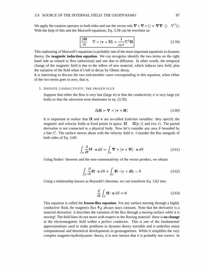
This rephrasing of Maxwell’s equations is probably one of the most important equations in dynamotheory, the magnetic induction equation. We can recognize identify the two terms on the righthand side as related to flow (advection) and one due to diffusion. In other words, the temporalchange of the magnetic field is due to the inflow of new material, which induces new field, plusthe variation of the field when it’s left to decay by Ohmic decay.It is interesting to discuss the two end-member cases corresponding to this equation, when eitherof the two terms goes to zero, that is.

1. INFINITE CONDUCTIVITY: THE FROZEN FLUX

Suppose that either the flow is very fast (large � ) or that the conductivity � is very large (orboth) so that the advection term dominates in eq. (3.59).

�� (3.60)

It is important to realize that � and � are so-called Eulerian variables: they specify themagnetic and velocity fields at fixed points in space: � � � � � � � and �

� � � �� . The partialderivative is not connected to a physical body. Now let’s consider any area

�bounded by

a line � . The surface moves about with the velocity field � . Consider the flux integrals ofboth sides of Eq. 3.60: �

�� (3.61)

Using Stokes’ theorem and the non-commutativity of the vector product, we obtain:�� < �

�� (3.62)

Using a relationship known as Reynold’s theorem, we can transform Eq. 3.62 into:�� " (3.63)

This equation is called the frozen-flux equation. For any surface moving through a highlyconductive fluid, the magnetix flux

� �always stays constant. Note that the derivative is a

material derivative: it describes the variation of the flux through a moving surface while it ismoving! The field lines do not move with respect to the flowing material: there is no changein the electromagnetic field within a perfect conductor. This is one of the fundamentalapproximations used to make problems in dynamo theory tractable and it underlies manycomputational and theoretical developments in geomagnetism. While it simplifies the verycomplex magneto-hydrodynamic theory, it is now known that it is probably not correct. In


particular, if one wants to describe effects on a somewhat longer time scale, say longerthan several tens of years, one has to account for diffusion. However, for the description ofrelatively fast processes the application of the “frozen-flux” approximation is appropriate.

2. NO FLOW: DIFFUSION (DECAY) OF THE FIELD

Suppose that either there is no flow ( � � �) or that the conductivity � is very low. In both

cases the diffusion term in eq. (3.59) (�� ) �E� �

' � � ) will control the temporal variation in� . Effectively, eq. (3.59) can be rewritten as the (vector) diffusion equation

� � � � �� ) �E� �

' � � (3.64)

which means that H (=� � � ) decays exponentially with time at a rate

�� ) �E� �

' � � �', where

� is the decay time of the field. The decay time � increases with conductivity � , but unlesswe consider a superconductor, the field will decay. For the earth, this case would representthe situation that the main field is due to some primordial field and that no core flow isinvolved. For realistic numbers, the geomagnetic field would cease to exist after severaltens of thousands of years.

This is a very important conclusion, since it means that the magnetic field has to be sus-tained! because otherwise it dies out relatively quickly (on the geological time scale). Thisis one of the primary requirements of a geodynamo: it has to sustain itself! (by means ofscenario 2)

The diffusion equation also shows that the depth to which the ambient field can penetrateinto conducting material is a function of frequency. This is an important concept if onewants to use fluctuating fields to constrain the conductivity or if one studies the propagationof changes in core field through the conducting mantle and crust.

Consider a magnetic field that varies over time with a certain frequency � (in practice wewould use a Fourier analysis to look at the different frequencies), diffusing into a half-spacewith constant conductivity � . It is straightforward to show that a solution of the vectordiffusion equation is

� � � )��

�� (3.65)

with

� N�

� � � ) P ��(3.66)

the skin depth, the depth at which the amplitude of the field has decreased to 1/e of theoriginal value. The skin depth is large for low frequency signals and/or low conductivityof the half-space. Rapidly fluctuating fields do not penetrate into the material. (I gave theexample of swimming in still pond: on a winter day you would - probably - not consider togo swimming even on a nice day with a day time temp of, say, 20 � C, whereas you mighton a summer day with the same temperature. The point is that the short period fluctuationscontroled by night-day cycles do not penetrate deep into the water; the temperature of thewater that makes you decide whether or not to go for a swim depend more on the long period

3.9. SOURCE OF THE INTERNAL FIELD: THE GEODYNAMO 89

variations due to the changing seasons.) The rapid fluctuations of the external field are usedto study � in the upper mantle (z � 1000 km) and the core field is used to study � in thelower mantle.

Geodynamo

So we have a large volume of highly conducting liquid (metallic iron) that moves rapidly in theEarth’s outer core. The basic idea behind the geodynamo is that the rapid motion of part of theliquid in an ambient magnetic field generates a current that induces a secondary magnetic fieldwhich is largely carried along in the fluid low (”frozen flux”) and which reinforces the originalfield. In principle, this concept can be illustrated by Faraday’s disk generator.Excess of the light constituent in the outer core is released at the inner core boundary by progres-sive freezing out of the inner core. The resulting buoyancy drives compositional convection in theouter core, and the combination of convection and rotation produces the complex motion neededfor self-excited dynamo action. The rotation effectively stretches the poloidal field into toroidalfield lines (the � -effect). Most geodynamo models require a strong toroidal field, about 0.01 T (or100 Gauss), even though this field cannot be observed at the Earth’s surface. These toroidal fieldlines are warped up or down due to the radial convective flow (assuming “frozen flux”): as a resultof the Coriolis force this results in helical motion, which, in fact, recreates a poloidal componentfrom a toroidal one (this is know as the � -effect). The rotation controls the motion in such a waythat the dipole field is stronger than any other poloidal component and, averaged over a sufficienttime, coincides with the Earth’s rotation axis.

Intermezzo 3.5 SPHEROIDAL, TOROIDAL, POLOIDAL

The following will help understanding the terminology. An arbitrary vector field � on the surface of a unitsphere can be represented in terms of three scalar fields � , � and � as follows:

� � �� (3.67)

where the operator � is the dimensionless surface gradient on the unit sphere, formed by taking theprojection of the “real” gradient onto the plane tangent to the surface.A vector field of the form �� is said to be spheroidal (i.e. having both radial and tangentialcomponents) whereas one of the form � �� is said to be toroidal. A toroidal field is purely tangential.It resembles a torus which is purely circular about the � -axis of a sphere (i.e., follows lines of latitude). Thecurl of a toroidal field (its rotation), is, by definition, poloidal. A poloidal field resembles a magneticmultipole which has a component along the � -axis of a sphere and continues along lines of longitude.


3.10 Crustal field and rock magnetism

From spherical harmonic analysis it is clear that short wavelength magnetic anomalies must havea shallow origin. Within the outer few km of the Earth are rocks with minerals that have ferromag-netic properties. The study of these rocks and their magnetization has two important applicationsin geophysics:

� These rocks distort the magnetic field due to the core and the local field can be used toinvestigate crustal structures. (Note that we have seen that the downward continuation ofthe crustal field obscures the higher degree components of the core field at the CMB).

� Some of these rocks exhibit permanent magnetization (= remanent magnetization with verylong, i.e. � U � yr, relaxation times) and effectively provide an invaluable record of the pasthistory of the magnetic field and the relative motion of tectonic units � paleomagnetism.

Before discussing paleomagnetism we need to know some of the basics of rock magnetism inorder to study the local field. In particular:

� What are the possible sources of magnetization and what are the conditions that result in astrong, stable magnetization?

� What are the important rock types and minerals?

� What are the essential aspects of sample preparation before any accurate paleomagneticmeasurements can be done? (I will discuss this only briefly.)

The physics of the magnetization of an assemblage of rocks is not simple. Traditionally, the Frenchhave played a major role in research of magnetism, and L. Neel was awarded a Nobel prize for hispioneering theoretical work on rock magnetism.

3.11 Magnetization

Strength of magnetization: permeability and susceptibility

Let’s start from one of Maxwell’s equations. Remember that� � �� < �� (3.68)

where � is the magnetic field strength and � � � � and � are the macroscopic current and dis-placement current densities, respectively. Let’s forget about the displacement current density fora moment (like in the magnetohydrodynamic assumption). The displacement current is usuallyspread out over large areas and hence � and also

�� can be neglected.

In vacuum, the only current one needs to worry about is the macroscopic currents. In real materials(such as rocks), the atoms and molecules that make up the substance are like little magnetic dipoleswith a dipole moment � : a hydrogen atom, for instance is little more like the primitive currentloop we started the definition of the magnetic dipole moment with. The magnetization of asubstance is defined as the volume density of all these little dipole vectors:

3.11. MAGNETIZATION 91

� � �A�� ) �� (3.69)

One can express the density of microscopic molecular currents � �� through this magnetizationvector as follows: � � �� (3.70)

Hence we can rewrite Eq. 3.68 with both the macroscopic and microscopic current densities asfollows (using $ � � ) � ): � $ � � ) � � � � < � ) � � � (3.71)

which leads to � N$� ) � � P ��

� (3.72)

Comparison with Eq. 3.68 shows that the field strength in a material is given with respect to themacroscopic currents as:

� � $� ) � � � (3.73)

It is customary to associate the magnetization not with the magnetic induction, but with the fieldstrength. It is assumed that this relationship exists:

� �� (3.74)

The Greek capital letter chi ( � ) is used for the magnetic susceptibility tensor. It relates the threecomponents of the internal magnetization to the applied field, hence it is a second-order tensor (amatrix). This is usually a complex function, as � may depend on anything — temperature, grainsize, � , strain and so on. It can be negative, too. If � is a tensor, then � and

�need not be

collinear. Usually, the assumption of magnetic isotropy is made, and Eq. 3.74 is approximated bya scalar relationship:

� �� (3.75)

Now � and�

are collinear, but the magnitudes and sense are regulated by the value and signof � . Because both � and

�have dimensions of the field, � is a dimensionless constant: the

magnetic susceptility.So Eq. 3.73 reduces to

� � $� ) � U <�� $

� ) � � (3.76)

A quantity � was defined which is called the relative permeability of the substance. In vacuum,� �VU , � �� and

� �� — no bound charges exist in free space.When a magnetic body is placed in an external magnetic field � the density of the field linesinside the body depends on the strength of � and on the magnetization

�induced by � . Thus,

the magnetic susceptibility � indicates the ease with which a magnetic body can be magnetized inan external field.


Types of magnetization

The magnetization of a mineral is controlled by intrinsic (i.e., material dependent) magnetic mo-ments of electrons spinning about their axes (spin dipole moments) or the motion of electronsin their orbits about the atomic nuclei (orbital dipole moments). There are several types of spininteractions that give rise to different magnetic effects. The following is a brief summary.

Remanent or Induced? (Konigsberger ratio)

When we talk about magnetization, we can broadly identify two types:

1. Induced magnetization,� � , which occurs only if an ambient field � is present and de-

cays rapidly if this external field is removed. This induced field is very important in oreexploration.

2. Remanent magnetization,��

, which is the part of initial magnetization that remains afterthe external field disappears or changes in character.

��forms the record of the past field

and is the type of magnetization that makes paleomagnetism work.

In natural rocks, the ratio between the two is known as the Konigsberger ratio�

� � � �� (3.77)

Rocks with high�

tend to be magnetically stable and are good recorders of the ancient geo-magnetic field. (I just remark at this stage that the strength of

� �� does not only depend on the

composition (more precisely the type op magnetic minerals) but also on the grain size, and whetherthe magnetic particles consist of single or multiple grains). Rock types with high

�are most of

the mafic rocks, such as basalt and gabbro, and also granite. Limestone, for instance, typically hasa very small Konigsberger ratio.Examples of induced magnetization are diamagnetism and paramagnetism. The fields are weakand decay rapidly when the external field is removed (by means of diffusion).DIAMAGNETISM

All materials tend to repel the magnetic field lines of force so that the density of field lines withinthe body ( � � �

�) is smaller than outside (

� �� ):�

� � � ) � U <�� ) � � � � U <�� U � � (3.78)

This effect, which is controlled by orbital dipole moments can be explained by Lenz’s Law,which states that the field produced by a conductor moving an a magnetic field tends to oppose theexternal field. Here, the induced field produced by the electron spin tends to oppose the externalfield. Even though all materials are diamagnetic, in some the effect is completely overshadowedby much stronger effects such as ferrimagnetism.Diamagnetism is a weak effect

�� U �

�so that

��

��

�.

Owing to diffusion, the original state is quickly restored when the external field � would beremoved unless the conductivity � is very large (superconductors) so that the diffusion (whichscales as U�� , see magnetic induction equation) can be neglected.PARAMAGNETISM


Intrinsic paramagnetism is relevant for only a small class of materials, but most magnetic min-erals are paramagnetic above the curie temperature (see below). Paramagnetic minerals tend toconcentrate the lines of force so that the induced internal field $ is larger than the external field� . �

� � � ) � U <�� ) � � � � U <�� U � � (3.79)

Electrons spin in opposite directions giving rise to spin dipole moments in opposite directions. Thespins are arranged in pairs so that the net effect of the magnetic dipoles is zero. However, if thenumber of orbital electrons is odd there is a small net magnetic moment that can be aligned withthe external field. This is known as paramagnetism. Atoms with an even number of electrons tendto be diamagnetic and those with an odd number tend to be paramagnetic. Like diamagnetism, theeffect is small:

�� U � � so that

��

��

�.

The susceptibilities of para- and diamagnetic minerals are virtually independent of the ambi-ent field (see linear behavior in the above diagrams) but paramagnetism is strongly temperaturedependent because thermal fluctuations tend to disorient the alignment with the applied field (com-petition between thermal energy that tends to destroy alingment and magnetic energy that tends tocreate it). The Curie Law states that paramagnetic susceptibility is inversely proportional to theabsolute temperature.

FERRO- AND FERRI- MAGNETISM

This type of magnetism can result in a remanent magnetization which remains even after theambient field � changes at a later time. The susceptibility of ferro- and ferri- magnetic minerals


depends strongly on the applied external field, but in general � � . In ferromagnetic mineralsthe electron spins line up spontaneously. Perfect line-up occurs only in a few metals, such asmetallic iron in the Earth’s core, and alloys; in other minerals, such as magnetite, the line-up is notcomplete which results in ferrimagnetism.

Which minerals are important?

The most important rock-forming minerals with magnetic properties are

magnetite �� 2 �� 2 � �hematite �� 2 � � (can be formed from magnetite by oxidation)ilmenite ��

A� �

The magnetic properties of these magnetic minerals and the continuous series of solid solutionsbetween them can be conveniently displayed in ternary diagram of the ��

� ��A� ��

system:

�� <�� ; �� A � � �� <�� A � ; ulvospinel �� A � � �� <�� A � �The titanomagnetite solid solution series � from magnetite � ulvospinel consists of strongly mag-netic cubic oxides. The titanohematite series

�(from ilmenite � hematite) consists of weakly

magnetic rhombohedral minerals. Some important properties of the minerals in the ternary dia-gram are: Curie temperatures decrease from right to left; generally, the susceptibility increasesfrom right to left. Even though, for instance, magnetite has a lower susceptibility than, sayulvospinel , it is more suitable for paleomagnetic studies, because uit maintains its remanenceup to much higher temperatures.


Intermezzo 3.6 MAGNETIC HYSTERESIS

When a ferromagnetic body (or an assemblage of asymmetric single grains) is placed in an ambient fieldthe magnetization will initially increase linearly with the strength of the ambient field. This linear part ofthe magnetization is reversible and the sample will return to its original state when the ambient field isremoved. The initial susceptibility is then defined as � � � � �� . If the external field increases instrength saturation will occur, for instance because no more magnetic domains within a rock can be aligned,and the magnetization � rotates into the direction of the ambient field � . This part of the process in non-reversible: if the ambient field is removed, there may be some relaxation (the reversible part) but a remanentmagnetization �� will remain. If the external field would change directions a hysteresis the magnetizationwould follow a hysteresis curve. The strength of the magnetization depends on grain size and temperature:the larger the single grains and the lower the temperature, the wider the hysteresis curve and the stronger(”harder”) the magnetization. See Figure ??.

Magnetic domains and influence of grain size

In bulk magnetic material, say, magnetite, the regions of spontaneous magnetization (magnetic do-mains) are arranged in patterns to form paths of magnetic flux closure with neighboring domains,so that no net effect is observed. This is known as the demagnetized state. The size of the singledomains in such agglomerates depends on susceptibility and are larger in hematite than in, say,the titanomagnetites (see below). When placed in an ambient field � the boundaries between thedomains may migrate in such a way as to enlarge the domains that are favorably oriented with


Figure 3.8: Magnetic hysteresis.

respect to the external field, and this may cause magnetic remanence. The process of cell bound-ary migration is (energetically speaking) an easier process than the realignment of the direction ofmagnetization and, as a consequence, large multidomain grains are magnetically ”soft” (i.e. notstable over long periods of time and sensitive to later changes in the orientation and strength of theambient field).In contrast, single domain grains have the same direction of spontaneous magnetization through-out, and if they are not in contact with neighboring grains they cannot form closed loops and theycan more easily be magnetized to saturation.At high temperatures (or for very small single grains) the kinetic energy, or the thermal agitation,of the system can be too large for any kind of cooperative process to be effective and the electronspins are not aligned but cancel out. In this state the rocks are paramagnetic, and magnetizationcan only be induced by an external field. If the assemblage is given a magnetization at time )the (induced) magnetization decays a � �

�� ) where � ) , the relaxation time, varies directly as grain

volume (� � ) and inversely as temperature

�. In other words, the relaxation time becomes shorter

exponentially with increasing temperature. When the relaxation time � ) is very large (say 10 & year)the remanence is said to be permanent. The dependence of the relaxation time on temperature andthe grain size of single grain particles can be illustrated schematically:When the rock sample cools, the relaxation time and the susceptibility (Curie’s Law) increase (thewidth of the hysteresis curve increases) and there comes a point, at

� � ��, the Curie temperature

(after Pierre Curie), at which the thermal agitation is no longer large enough to prevent alignmentof the magnetic moments. At this point the assemblage of grains acquires a magnetization in thedirection of the ambient field, which upon further cooling becomes frozen in. This is known asThermoRemanent Magnetization (TRM).The transition from a state of paramagnetism to TRM is not instantaneous and typically occursover a certain temperature range. The process of acquiring TRM consists of a series of partialthermo remanent magnetizations, each acquired in a given temperature range, say,

� ' � � � � ,and each preserving a record of the ambient field in that time interval. Reheating to

� ' would not

3.12. OTHER TYPES OF MAGNETIZATION 97

Figure 3.9: Magnetic domains in grains.

destroy that part of the remanent magnetization, but reheating to� would. This, in fact, underlies

the principle of thermal cleaning. For most rocks containing a single, magnetic constituent thepartial TRM acquired at about 50 � below the Curie point is dominant. If the assemblage consistsof a series of minerals with different Curie points the initial remanence can easily be overprintedwith secondary components reflecting the field direction at some later time. For several miner-als along the solid solution lines, the ternary system described above gives values of the Curietemperature Tc above which ferro- or ferrimagnetism is not possible. In general the Curie tem-perature decreases from right to left, i.e., hematite to ilmenite and from magnetite to ulvospinel.For hematite

� �=680 � , for magnetite

� �=580 � , and for metallic iron (core!)

� �=770 � .

It is important to realize that the strongly magnetic minerals do thus not necessary result in astrong and stable (= long lasting) magnetization since their Curie temperatures can be so smallthat the original magnetization can easily be altered during later thermal events (for some magneticminerals this can happen at room temperature). Conversely, the weakly magnetic minerals may,in fact, produce very stable magnetization. Weak and strong refers to the value (small, large) ofthe magnetic susceptibility; stability refers to the time scales over which the magnetization canlast, and this is more a function of grain size and the composition-dependent Curie and blockingtemperatures.

3.12 Other types of magnetization

TRM – THERMOREMANENT MAGNETIZATION

In terms of later overprints, it is good to realize that the direction of TRM can be reset if thetemperature is raised to above the relevant Curie temperature during some later thermal event.Upon cooling a new TRM is frozen in. Often, however, reheating will also reset the dating clockssince the closure temperatures for minerals typically used for radio-isotope dating are often lower


Figure 3.10: Temperature dependence of Curie tempera-ture.

Figure 3.11: Saturation magnetization.

than the Curie temperatures for the iron oxides. (This is generally true for the minerals involvedin K–Ar and Rb-Sr dating – hornblende (530 � ), muscovite (350 � ), biotite (280 � ), apatite ( 350 � ),but U-Pb dating is more borderline with the closure temperatures for several important mineralsexceeding 600 � , for instance Zircon at 750 � ). As a consequence, the data can still be used forpaleomagnetism; the magnetization just relates to a later thermal event.DRM – DETRITAL REMANENT MAGNETIZATION

When igneous rock is eroded and the magnetic constituent is deposited in sufficiently still waterthe magnetic grains that carry TRM from previous events may become aligned in the ambientfield. Since this type of magnetization is in fact based on previous TRM it can be a stable and’strong’ magnetization which can be useful, provided that the time of deposition can be determinedaccurately. There are, however, several complications, for instance, the change in any lineationdirection due to compaction may result in an underestimation if the inclination

Mand this would

underestimate the paleolatitudes.CRM – CHEMICAL REMANENT MAGNETIZATION

Some ferro- or ferri- magnetic minerals may be formed long after the rocks first cooled belowthe Curie temperature. For instance, magnetite may oxidize to hematite which then can settle ascement in the matrix between the grains. Conversely, magnetite may be formed from hematite ina reducing environment. Upon the chemical reactions and renewed deposition the minerals are

3.13. MAGNETIC CLEANING PROCEDURES 99

re-magnetized in the then ambient field. In these examples the CRM is very strong. Since theacquisition of CRM does not involve any reheating up to the Curie temperature (which is typicallyabove the blocking temperature for radioisotope dating!) it is not possible to put a time tag on andit can not be used for paleomagnetism.IRM = ISOTHERMAL REMANENT MAGNETIZATION

Exposure of a magnetized sample to very strong field even without increasing the temperature (forlong enough time) can result in the re-arrangement of part of the initial TRM. IRM is characterizedby a very narrow hysteresis curve so that the magnetization is relatively “weak”. An importantsource for IRM are lightning strikes.VRM – VISCOUS REMANENT MAGNETIZATION

Results from the slight reorganization of the magnetic moment in some grains if the grain isexposed to an ambient field for a very long time. The external field can ”diffuse” into the sample,in particular if both � and � are large.

3.13 Magnetic cleaning procedures

For paleomagnetic purposes, the overprints by the other types of magnetization are thus a nuisance;if the secondary remanence is ”soft” their effects can be removed by techniques collectively knownas ”magnetic cleaning”. Cleaning is based on the principle that the soft components are destroyedwhile the strong original TRM or DRM is preserved. This can not always be guaranteed and, as aresult, the intensity of the field after cleaning may be unreliable.

� Alternating field cleaning (a.f. cleaning). Makes use of hysteresis properties of ferro- andferri- magnetic minerals. The strength of a particular magnetization is determined by thewidth of the hysteresis curve, which represents the field of opposed direction that wouldhave to be applied to reduce the remanence to zero. The field is often referred to as thecoercive force � � (see hysteresis curve). In a.f. cleaning one exposes the field sample to analternating field with diminishing strength and the sample is rotated in all directions. Thisprocess wipes out all components with a strength � � that is less than the maximum fieldapplied. Of course, this only works if the primary component is stronger than that! Thisprocess must be performed in a laboratory set up where one compensated for the externalEarth field in order to avoid remagnitization along � � .

� Thermal cleaning. Makes use of Curie’s law and Curie temperatures. The field sampleis heated to a particular temperature to destroy magnetization of minerals with Curie tem-peratures smaller than that value. This is, of course, only useful if the component you’reinterested in has a higher Curie temperature than the temperature that is applied.

� Chemical cleaning: leaching or dissolving certain components of the rock, such a thehematite rich matrix in a sand stone.

In general, one applies progressively stronger cleaning agents to the sample until the remainingfield is stable and no longer changes in direction. The intensity of the original TRM/DRM will beobscured in the process!


3.14 Paleomagnetism

A primary objective of paleomagnetism is to determine the history of the geomagnetic field (for avariety of purposes!) and what is needed is (1) ”hard” (+stable) magnetization and (2) informationabout the time at which that magnetization was acquired. So, of the above mechanisms only TRMand DRM are useful since they have hard magnetization and the acquisition of the RMs can bedetermined (radio-isotope dating and stratigraphy, respectively).

Field practice: orientation of the sample

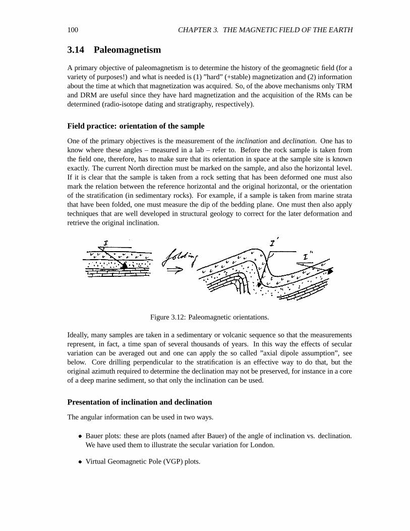
One of the primary objectives is the measurement of the inclination and declination. One has toknow where these angles – measured in a lab – refer to. Before the rock sample is taken fromthe field one, therefore, has to make sure that its orientation in space at the sample site is knownexactly. The current North direction must be marked on the sample, and also the horizontal level.If it is clear that the sample is taken from a rock setting that has been deformed one must alsomark the relation between the reference horizontal and the original horizontal, or the orientationof the stratification (in sedimentary rocks). For example, if a sample is taken from marine stratathat have been folded, one must measure the dip of the bedding plane. One must then also applytechniques that are well developed in structural geology to correct for the later deformation andretrieve the original inclination.

Figure 3.12: Paleomagnetic orientations.

Ideally, many samples are taken in a sedimentary or volcanic sequence so that the measurementsrepresent, in fact, a time span of several thousands of years. In this way the effects of secularvariation can be averaged out and one can apply the so called ”axial dipole assumption”, seebelow. Core drilling perpendicular to the stratification is an effective way to do that, but theoriginal azimuth required to determine the declination may not be preserved, for instance in a coreof a deep marine sediment, so that only the inclination can be used.

Presentation of inclination and declination

The angular information can be used in two ways.

� Bauer plots: these are plots (named after Bauer) of the angle of inclination vs. declination.We have used them to illustrate the secular variation for London.

� Virtual Geomagnetic Pole (VGP) plots.

3.14. PALEOMAGNETISM 101

Figure 3.13: Bauer plot.

From the measured inclination

Mand declination we can calculate (1) the magnetic co-

latitude (i.e., the angular distance from the paleo-pole to the sampling site) and (2) theposition of the paleomagnetic pole and the virtual (or apparent) geomagnetic pole (VGP).Let’s see how we can do that.

From the derivation of the potential of an axial dipole we know that the magnetic co-latitude � �can be calculated from the basic equation for paleomagnetism:

��B M � �

698� � � � � ! �

� �(3.80)

where�L�

is the magnetic latitude ( � � = 90 � -�L�

). We can also calculate the location of the poleby measuring out the angular distance � � in the direction of from North.

This can be done by means of stereographic projections, but we can also use the sine and cosinerules on a sphere (see Intermezzo).


Intermezzo 3.7 COSINE AND SINE RULES ON A SPHERE

Let � ,�, and

�be the angular distances between 3 points and � ,

�, and � the angles as indicated in Figure

3.14.The cosine rule for � and � is:

�� (3.81)

and the sine rule:

��

�� (3.82)

(Note that we used (�

, � ) instead of the ( � , � ) to be consistent with the use of D for declination.)

Figure 3.14: Cosine and sine rules on a sphere.

Let � , � , � be the longitude, co-latitude, and latitude of a point, and subscripts � and � indicate thepaleopole and the sample site, respectively ( � � and � � as above). Then we can apply the cosinerule for : 698�: �� 698�: � � 698�: �� < :�ACB � � :�ACB �� 698�: (3.83)

and �� 6 698�:

�698�: � � 698�: ��(< :�ACB � � :�ACB �� 698�: �� (3.84)

with � � � U � � (3.85)

The application of the sine rule gives the longitude of the paleopole relative to the longitude of thesample site: :�ACB � �:�AGB � �� 9� � :�ACB � �:�ACB

(3.86)� � � � � � ��6 :�ACB + :�ACB

:�ACB � �:�ACB �� H

3.14. PALEOMAGNETISM 103

Figure 3.15: Location of paleopole.

(Note that arcsin is double valued: one always has to check that one uses the correct solution).The coordinate ( � � , � � ) is the apparent position of the pole for a magnetic field if the field isdipolar. The pole determined from a single site is called the Virtual Geomagnetic Pole (VGP).An important result from paleomagnetism is that the non-dipole field almost completely averagesout over extended periods of time (10,000 yr +) and that the average of all the VGPs from rocksof about the same age cluster together about the rotation pole. The is summarized in the AxialDipole Assumption: if we consider sufficiently long time intervals the average VGP representsthe paleopole or the paleogeographic pole.

Figure 3.16:

It was soon realized that the paleogeographic poles did not coincide with the current rotation poleand that the poles determined from samples of a different age do not necessarily overlap. This


was initially interpreted as evidence that the poles must move, hence the (obsolete) name PolarWander. We now know that the poles are fixed and that the pole paths describe the relative motionof the landmass relative to the pole. A rotation of both the pole and the sample site (continent)about a rotation pole at the present-day equator at and angle of 90 � from ( � � , � � ) gives the situationat the time of magnetization (assuming normal direction of the field). For each separate tectonicunit, measurements from samples that are magnetized at different times determines give a seriesof VGPs which define a pole path , or apparent polar wander (APW) path.

Figure 3.17: Apparent polar wander paths.

Note that on VGP diagrams one plots the VGP position relative to a fixed landmass but in realitythe poles are the same and the landmass moves!The observation that the pole paths do not agree for different continents demonstrates that the con-tinents must have moved relative to one another � plate tectonic motion (old term: continentaldrift). Conversely, the difference in pole paths can be used to reconstruct these movements, andthis is one of the basic principles of plate reconstruction.

Ambiguities in determination of VGPs and in reconstructing past plate motion

The position of the VGP can thus be determined from measurements of the inclination and decli-nation. There are, however, two important ambiguities.

1. The position of the VGP ( � � , �� ) is invariant for variation in longitude of the sample site.The landmass can be anywhere along a small circle at an angular distance of � � aboutthe paleopole. Since many earth systems (for instance, climate) exhibit a high degree ofrotational symmetry and, thus, primarily zonal variation, this ambiguity is difficult to solve.

2. The declination in the sense used above is poorly defined. In addition to rotation about thepaleopole (which does not effect the calculation of the VGPs) the sample site may have beensubject to rotation around a vertical axis nearby or through the land mass. In the latter casethe uncertainty in the true declination means that the VGP can – in principle – be anywherealong a small circle at an angular distance of � � about the sample site. The true paleopolecan then be found by the intersection of many such small circles and VGP estimates. Thesame applies to data from drill cores since one does not know the declination.

Once the paleopole is known from many observations, this ambiguity disappears, and from theknown pole one can determine the magnetic (co-)latitude, or, in other words, the N-S motion ofthe sample site and the relative rotation about any axis other than the paleopole.

3.15. FIELD REVERSALS 105

3.15 Field Reversals

For Earth, a reversal can be defined as a globally observed change in sign of the gaussian coeffi-cient

5 ) ' that is stable over long ( � 5kyr) periods of time.What’s the relevance of studying field reversals?

� The alternating fields are recorded as magnetic anomalies in newly created ocean floor.This provides us with a fantastic dating device (the magnetic reversal time scale) and a verypowerful tool to track past plate motions.

� It may give us important clues and constraints for our understanding of core dynamics, thevery origin of the main field, and the possible mechanisms of core-mantle coupling.

� The magnetic field creates a protective shield for radiation from space (solar wind, for in-stance) and changes in intensity of the field may also change the effectiveness of this pro-tection. Major events in the evolutionary process have been linked to variations in paleo-intensity.

Figure 3.18: The magnetosphere.

� For navigation purposes it is important to know what’s going on with the field, for instancewhether it is going through a more rapid-than-average change.

Discovery of field reversals: a historical note

TRM was well known in the 19��

century. Evidence for field reversals was first reported in 1906when the French physicist Bernard Brunhes discovered that the direction of magnetization in a lavaflow and the adjacent baked clay was opposite of that of the current main field. Brunhes concludedthat the field must have reversed, but that explanation was not generally accepted. Recall that atthat time the origin of the main field was still a mystery. In fact, it was in the same year 1906that Oldham demonstrated the existence of a liquid core from seismological observations, and thatdiscovery triggered the development of geodynamo theory as we now know it. Later, in 1929Matuyama published similar observations as Brunhes, but these also attracted little attention. This


continued until well into the 50ies, by which time there was ample observational evidence for fieldreversals.

However, the necessity for field reversals was debated and a major proponent of an alternative ex-planation was the French physicist Neel who showed that under certain conditions ferri-magneticminerals could, in principle, be self-reversing. Self-reversal can happen in a situation where youhave a solid solution of magnetic minerals (or two at least) with different Curie temperatures (thinkof the hematite-ilmenite series). Then, when the sample cools the mineral with the highest Curietemperature, say mineral A, freezes in the ambient main field while the minerals with lower Curietemperatures are still in paramagnetic state. If these paramagnetic minerals are very close to min-eral A, the remanent field of A can induce a field in the other minerals that may be opposite of thedirection of the main field. This secondary field becomes frozen in when mineral B cools belowits own Curie temperature, etc. etc. In case the mineral with the lower Curie temperature has alarger susceptibility (and this is indeed the case for the minerals along the solid solution lines inthe ternary diagram!) the reversed field may dominate the combination of the ambient field andthe induced field in mineral A, and the net effect would be opposite in direction of the main fieldwithout requiring a reversal of that main field. Even though it has been shown experimentallythat self-reversal is possible, it requires very special physical conditions and it is NOT a plausiblemechanism to explain the by then (mid 50-ies) overwhelming evidence that reversals are quitecommon.

Study of baked clays (or thermal aureoles of igneous bodies in general) at many sites world widedemonstrated that the direction of magnetization in the igneous body and the contact aureole wereoften the same but did not coincide with that of the adjacent non-metamorphosed rocks. It wasfound that the rocks showing reversals grouped in specific age intervals, and this argument becameeven more convincing when accurate radiometric techniques such as K–Ar dating were applied.The reversals appeared to be rather global phenomena and could be traced in volcanic rocks aswell as in marine sediments. There appeared to be no chemical difference between the rocks theexhibited normal and reversed orientations.

By the time of the early 60-ies several important discoveries associated with sea floor spreadingresulted in the general acceptance of field reversals.

Outstanding questions

1. What happens to the dipolar field during reversals? Does the dipole field decay to almostzero before it is regenerated in the opposite direction, or is the dipole field perhaps weakenedbut still prominent during reversals? The measurement of paleointensity of the main field isdifficult and prone to large uncertainties (see also notes on ”magnetic cleaning”). Yet, it isnow well established that during reversals the intensity of the field reduces by at least a factorof 3. Recall that in the present-day field the dipole makes up for about 90% of the field andthat the non-dipole component is only about 10% . So although the field reduces to about30% of its original strength, the dipolar component cannot be neglected during reversals.These numbers are, however, not yet well constrained. Some data (and numerical models)suggest a reduction during reversal to about 10% of the original strength, which would eitherimply that the dipole component has become negligible or that if there still is a dipolar fieldalso the non-dipole components must significantly reduce in strength. The observationalevidence is problematic because [1] the non-dipole field at the surface is so much weaker

3.15. FIELD REVERSALS 107

than it is at the CMB and [2] because a reversal is a relatively short phenomenon (say 5,000yr) and it is hard to get the time resolution in volcanic or sedimentary strata.

2. A closely related question is: can a non-dipole field produce continuous VGP paths duringreversals? Are VGP paths random or are there are preferred longitudes along which theVGPs move from the one pole to the other, and what are the implications of the answer tothis question for our understanding of core dynamics and core-mantle coupling?

Mechanisms of reversals

The mechanisms of field reversals are still subject of spirited debate, but it is generally acceptedthat they are controlled by core dynamics. Some important constraints (and, indeed, the need forcore-mantle coupling) can be inferred directly from general properties of the geodynamo and fromstudying the (statistical) behavior of the field during and in between reversals.

1. It is important to realize that the geodynamo does not care about the sense of the field. Themagnetic induction equation

� � � � � � � � � � < � �� ) �E� �

' � � is invariant to achange in sign of � .

We have argued before that in the core we can largely ignore the diffusion term, and it isclear that the (sign) of the changes in magnetic field depend entirely on how the turbulentflow field � interacts with the magnetic field � .

2. The typical relaxation time of core processes is much longer than the time interval in whichmost reversals take place. If the field is not sustained by dynamo action, for instance if thevelocity � in the above equation goes to zero, the field will die out in several 10 � years. Therate of reversals must mean that the core field is actively destructed and regenerated. Partof dynamo theory is the complex interaction of and conversion between the poloidal and(unseen) toroidal field. Differential (radius dependent) rotation in the outer core stretchesthe poloidal field into a toroidal field; radial flow owing to compositional convection distortsthe purely toroidal field (and the coriolis force adds extra complexity in the form of helicalmotion) which gives a component along the poloidal field. It is conceivable that turbulenceproduces local changes in the direction of the helicity of the toroidal field and thus thepoloidal component, which may trigger a reversal.

3. Reversals are not simply extreme cases of secular variation even though the distinction isvague. Growth, decay, and drift of the non-dipole field and of the axial dipole are continu-ous, albeit possibly random, processes. Reversals, however, occur over time scales that arelonger than the typical secular variations, but much shorter than the average time intervalbetween reversals ( � U � yr). In other words, statistically speaking reversals do not occuras frequently as one might expect from the continuous (secular) fluctuations of the mainfield. It resembles a chaotic system that switches back and forth between two quasi-stablestates. This behavior is nicely illustrated by measurements of the inclination, declination,and intensity during a reversal that characterizes the lower boundary of the Jaromillo event(a short N event in the Reversed Matuyama epoch documented near a Creek in Jaromillo,Mexico:


3.16 Qualitative arguments that explain the need for core-mantlecoupling

There are compelling reasons to believe that the mantle and the dynamic processes in the mantlehave a strong influence on reversals (and thus perhaps on core dynamics in general). It is probablethat core flow is too turbulent and chaotic to be able to organize systematic patterns in field rever-sals. Reversals seem to be a random process in the sense that [1] N and R directions of the Earth’smagnetic moment occur equally often and [2] the probability that a reversal happens in the next

� years is independent of the time since the last reversal. However, as mentioned above, the averagetime interval between reversals is much larger than expected from the continuous fluctuations inthe field. Moreover, in the last 5 year several papers have been published that presented evidencefor preferred reversal paths of VGPs along meridians through the ’Americas’ and through eastAsia. The selection of the same VGP path over and over again seems to require that the core hassome ’memory’ about what happened many thousands of years ago, which is not very likely.

In contrast, the mantle, with its high viscosity has such ’memory’ since the mantle structure doesnot change much over periods that are smaller than 1 Myr. For this reason, investigators haveinvoked a strong influence of (or coupling with) the mantle. This coupling could be mechanical(topography on core mantle boundary) but that is not very likely. Alternatively, the coupling couldbe electro-magnetical; in this mechanism flux out of the core would be concentrated in regions

3.17. REVERSALS: TIME SCALE, SEA FLOOR SPREADING, MAGNETIC ANOMALIES109

where the conductivity of the lowermost mantle is lowest (see dynamo equation above!) andswept away from regions of high conductivity.Several investigators have related the patches of high and low mantle conductivity to lateral varia-tion in the thickness of the so called D” layer and this structure is likely to be influenced by flowin the entire mantle. This depicts a complex system where mantle convection controls the lateralvariation in thickness of the D” layer (thin beneath major downwellings (slabs) – Americas andeast Asia – and thicker beneath upwellings – plumes (central Pacific, Hawaii)) and thus – if D”is anomalously conductive – lateral variation in mantle conductivity that produces torques on thecore and creates ’windows’ for flux bundles from the core into the mantle. The research in thisexciting field is very much ongoing and no conclusive models has been developed yet.

3.17 Reversals: time scale, sea floor spreading, magnetic anomalies

We have talked in some detail about the implications of the reversals of the magnetic field for ourunderstanding of core dynamics and core-mantle coupling. This is a field of active research: rapidprogress is being made, but many outstanding questions remain to be answered. About 30-35 yearsago (first half of the 60-ies) the reversals of the main field played a central role in the developmentof the concept of sea floor spreading, which resulted in the acceptance of plate tectonics.To appreciate the line of thoughts it is good to realize that by the end of the 50-ies there wasno agreement on the issue of field reversals, even though an increasing number of scientists hadaccepted the idea. At the same time, continental drift was still hotly debated. Since the idea wasfirst clearly postulated by Alfred Wegener in 1912 it had been advocated by many scientists, forexample the South African DuToit, but, in particular, in the US the concept met with continuedresistance. A central issue was the driving force and the mechanism of continental drift; one didnot believe it possible that continents would plow their way through the mafic and strong oceaniclithosphere.

1. Initially, the evidence for reversals was mainly based on land samples of volcanic rocks.It was recognized that rocks with the same magnetic polarity grouped into distinct timeintervals, and the boundaries of these time windows could be dated accurately with radio-metric methods. The first Geomagnetic Polarity Time Scale (GPTS) was based on K–Arand � ) Ar/ � �

Ar dating of rocks less than 5 Ma old. Based on the first time scales one definedepochs as relatively long periods of time of mostly one polarity, and events as relativelyshort excursions or reversals of the field within the epochs. The first (= most recent) epochsare named after some of the pioneers in geomagnetism (Brunhes, Matuyama, Gauss, andGilbert); events are typically named after the location where it was either first discoveredor where it is best represented (Jaromilla creek, Mexico; Olduvai gorge, Tanzania). Thecurrent epoch is referred to as ”normal” (or ’negative’ since the magnetic moment directionis opposite of the angular moment direction). As more data became available the time tableswere refined and it became clear that the distinction between epochs and events is not souseful.

2. In the early 60-ies, marine expeditions and geomagnetic surveys resulted in the first detailedmaps of magnetic anomalies at the ocean floor. A ”stripe” pattern formed by alternatingstrength of the magnetic field (the anomalies were made visible after subtracting the valuesof the reference field (IGRF)) was documented for the Pacific sea floor off the coast of


Oregon, Washington, and British Columbia (Raff & Mason, 1961), and for the Atlantic justsouth of Iceland. The origin of this pattern was, however, not known. Explanations includedthe lateral variation in susceptibility owing to variations in composition or changes in stressdue to buckling (’folding’) of the oceanic lithosphere (it was known since the large 1906earthquake in San Francisco that changes in the stress field can influence magnetization).

3. At about the same time, Dietz (1961) and Hess (1962) postulated the concept of sea floorspreading. Not as an explanation for the magnetic anomalies, but rather as a way out ofthe long standing problem that continental drift seemed unlikely because continents can-not move through the oceanic lithosphere. Dietz and Hess realized that the oldest parts ofoceanic sea floor were less than about 200 Ma old, which is more than an order of magnitudeless than the age of the oldest continental rocks. This suggests that oceanic lithosphere isbeing recycled more efficiently than continental material. These scientists proposed that seafloor is generated at mid oceanic ridges (where pillow lavas had been dredged and high heatflow measured) and then spreads away carrying the continents with them. So the continentsmove along with the ocean floor, not through it!!

3.18. MAGNETIC ANOMALY PROFILES 111

In 1963 Vine and Matthews and, independently, Morley, put these ideas and developments(1-3) together and correctly interpreted the magnetic anomalies at the sea floor: new oceanfloor is created at mid oceanic ridges � the basalt cools below the curie temperature andfreezes in the direction of the then current magnetic field (normal (N) or reversed (R)) � theN-R pattern spreads away from the ridge. In this way the ocean floor acts as a tape recorderof the polarity of the Earth’s magnetic field in the past. Initially, the time table based onland volcanics was correlated with the stripe pattern in the oceans, but this correlation wasrestricted to the past 5 Ma. Later, paleontological data (the fossil record) was used (alongwith radiometric calibration of land volcanics)) to extend the reversal time scale to oceanfloor of Jurassic age ( 160 Ma). This was first done in the south Atlantic where the timescale was extended to 80 Ma by assuming that the rate of sea floor spreading was constantin that time interval, an assumption that was later justified). With the increasing amount ofdata, the time scale is continually being updated. The time scale is very important for twomain reasons:

� Using the GPTS allows the calculation of sea floor spreading rates by measuring thedistance between identified lineations.

� Identification of the magnetic pattern of the sea floor and matching with the time scalecan be used to date a piece of oceanic crust.

3.18 Magnetic anomaly profiles

In order to exploit the time scales (for instance for points (a) and (b) above) one must be ableto identify and interpret magnetic anomalies, or, more specifically for marine surveys, magneticprofiles due to a succession of magnetic anomalies with reverse polarity. In the interpretation oneusually tries to find a combination of N and R ’blocks’ that best matches the observed profile.This is easier said than done. A visual inspection of any of the profiles used as illustrations in, forinstance, it can be demonstrated that the relationship between the simplified block models and thecorresponding magnetic profiles is far from trivial. The magnetic profiles look more complex thanyou would expect from the simple block models, and this is true not only for real data but also forthe synthetic (computer generated) profiles.In the first place, the real sea floor is not magnetized in the form of regular geometric bodies.The geological processes at work in a mid oceanic ridge environment are complex and so are theresulting patterns of magnetization. In particular, the creation of new ocean floor in the so calledemplacement zone is an irregular process that is not necessarily symmetric across the ridge axis.Also the spreading rate has an effect in that fast spreading (Pacific rise) results in wide zoneswith the same magnetization which facilitates identification, whereas slow spreading (Atlantic)produces narrow anomalies with poor separation of the anomalies, which complicates the analysis.But even for a regular alternation of N and R polarity, say in a computer model, the magneticprofiles can be complicated. This is mainly due to the dipole character of the magnetic field asopposed to the monopoles in gravity, which means that the orientation of the anomaly plays animportant role.Before we look at this in more detail, let’s define what we mean by a ”magnetic anomaly” in thecontext of marine surveys. At sea one uses proton precession magnetometers (see, for instance,Garland, 1979) that are towed behind the ship. These instruments make use of the precession ofhydrogen atoms after a strong (artificial) ambient field generated by a current in a coil surrounding


a contained with many hydrogen atoms (e.g., water!) is switched off. When the initial field thataligns the hydrogen dipole moments is switched off the hydrogen atoms precess with a frequencythat depends on the strength of the ambient field. The precession induces a current in the coil,which can be measured.) Precession magnetometers measure the magnitude of the total magneticfield, not its direction (which means that they do not have to be orientated themselves!) and havea sensitivity of about 1 nT. The magnetic anomalies are determined by subtracting the IGRF fromthe observed values.In vector notation, the total field $ is given by the contributions of the main field (the core field)$ � and the magnetized body

$ :

$ � $ � < $ (3.87)

But the scalar magnetometer measures� � � $ � � � � < � (3.88)

with � the magnetic anomaly.

� � �$� � � $V� $ � ��

$ � � $ � < � $ � � $ < $V� $ �� (3.89)

� � � � � < � $ � � $ < � � ��Typically,

�is of the order of several hundreds of nT whereas

� �is of the order of 20,000 to

60,000 nT. Therefore we can safely neglect � so that� � � � � < � $ � �

$ �� U < �

�$ � $ � $ � � �

' � �� (3.90)

with the unit vector�$ � in the direction of $ � . The second term is small so that this expression

can be expanded in a binomial series�� U < $ � $ � $ � � �' � � � � < �$ � � $ (3.91)

and we define the magnetic anomaly � , see (3.88) as

� � � � � � � �$ � � $ (3.92)

In other words, the only components of the local field $ that we measure is the one parallel to

the direction of the ambient (core field). A vector diagram shows that this is a good approximationsince

� � � �. (For a dipole, the field is given by the gradient of the potential

$ � � � � �� ) � � � � �

' � � �� .)


Let’s consider some examples in which $ � is approximated by an axial dipole. Assume an in-finitely long block (lineation) that is magnetized in the direction of the ambient Earth field. Themagnetization direction can be decomposed into components parallel and perpendicular to thestrike of the block. It can be shown that the component

� �to the strike does not contribute to

a magnetic anomaly since the infinitely small dipoles that make up the anomalous structure alllie ’head-to-toe’ and cancel out except for the ones near the end (which infinitely far away (inother words, the field lines never leave the body). In this geometry, the magnetized body only hasmagnetization in the directions � to the strike (say, in the � and � direction). Consequently, aN-S striking anomaly magnetized at the equator will always have � � �

$ � � $ � since $ is

orthogonal to $ � (or, more precisely, there is no non-zero component of $ in the direction of�

$ � . In contrast, lineations magnetized at the pole and measured at the pole have�$ � � � $ so that

there will be a strong signal centered over the anomaly.

The effect of the orientation (which theoretically speaking gives rise to a phase shift) presentsitself as a skewness of the anomalies (see diagram) which can be corrected for (for instance byreducing the anomaly to the pole, see diagram).

In addition to these distortions due to the phase shift there’s the effect of amplitude modulation.Amplitude modulation consists, in fact, of two contributions:


1. usually, the magnetized body (at the ocean floor) is several km beneath the vessel. Theobserved magnetic field thus represents the upward continuation of the field at the source.As a result of the U�� decay of the field there is significant spatial attenuation of the highfrequency components. Sharp contrasts will be observed as more gradual transitions.

2. Since the magnetized body can be thought to consist of dipoles a homogeneously magne-tized lineation will only display a magnetic anomaly near its ends; in between, the plus andminus poles cancel out (same argument as above) and no anomalous field is measured. Thisresults in an effect known as sagging. See diagram on next page.

Chapter 3 campo de la tierra magnetico

Documents

Transcript of Chapter 3 campo de la tierra magnetico