Chapter 17 Reservoir Simulation - NTNUcurtis/courses/Reservoir-Recovery/2018... · 2018-04-05 ·...
40
V-1398 Petroleum Engineering Handbook-Vol. V Joseph, C. and Pusch, W.H.: "A Field Comparison of Wet and Dry Combustion," JPT (Septem- ber 1980) 1523. Koch, R.L.: "Practical use of combustion drive at West Newport field," Pet. Eng. (January 1965). Martin, W.L., Alexander, J.D., and Dew, J.N.: "Process Variables of In Situ Combustion," Trans., AIME (1958) 213, 28. Meldau, R.F., Shipley, R.G., and Coats, K.H.: "Cyclical Gas/Steam Stimulation of Heavy-Oil Wells," JPT (October 1981) 1990. Moss, J.T., White, P.O., and McNeil, J.S. Jr.: "In Situ Combustion Process-Results of a Five- Well Field Experiment in Southern Oklahoma," Trans., AIME (1959) 216, 55. Olsen, D. and Sarathi, P.: "Field application of in- situ combustion," Report No. NIPER/BDM 0086, U.S. Dept. of Energy, Washington, DC (1994). Showalter, W.E. and Maclean, A.M.: "Fireflood at Brea Olinda Field, Orange County, Calir- nia," paper SPE 4763 presented at the 1974 SPE Improved Oil Recovery Symposium, Tulsa, 22-24 April. Showalter, W.E.: "Combustion-Drive Tests," SPEJ (March 1963) 53; Trans., AIME, 228. Terwilliger, P.L. et al.: "Fireflood of the P2-3 Sand Reservoir in the Miga Field of Easte Venezuela," JPT (January 1975) 9. Widmeyer, R.H. et al.: "The Charco Redondo Thermal Recovery Pilot," JPT (December 1977) 1522. Williams, R.L., Jones, J.A., and Counihan, T.M.: "Expansion of a Successl In-Situ Combus- tion Pilot in Midway Sunset Field," paper SPE I 6873 presented at the 1987 SPE Annual Technical Conference and Exhibition, Dallas, 27-30 September. SI Metric Conversion Factors 0 API 141.5/(131.5 + 0 API) =g/cm 3 bar x 1.0* E+05 = Pa bbl X 1.589 873 E-01 = ! 3 Btu x 1.055 056 E+00 =kJ Cp X 1.0* E-03 =Pa·s ft X 3.048* E-01 =m ft 3 X 2.831 685 E-02 =m 3 O F ( ° F - 32)/1.8 = o c O F ( ° F +459.67)/1.8 = K kW-hr x 3.6* E+00 = J lbm x 4.535 924 E-01 = kg psi X 6.894 757 E+00 =kPa *Conversion factor is exact. Chapter 17 Reservoir Simulation Rod P. Batycky, Marco R. Thiele, StreamSim Technologies Inc.; K.H. Coats, Coats Engineering Inc.; Alan Grindheim, Dave Ponting, Roxar Software Solutions; John E. Killough, Landmark Graphics; Tony Settari, U. of Calgary and Taurus Reservoir Solutions Ltd.; L. Kent Thomas, ConocoPhillips; John Wallis, Wallis Consulting Inc.; J.W. Watts, Consultant; and Curtis H. Whitson, Norwegian U. of Science and Technology and Pera 17.1 lntroduction-K.H. Coats The Merriam-Webster Dictiona,y defines simulate as assuming the appearance of without the reality. Simulation of petroleum reservoir perrmance rers to the construction and operation of a model whose behavior assumes the appearance of actual reservoir behavior. The model itself is either physical (r example, a laboratory sandpack) or mathematical. A mathematical model is a set of equations that, subject to certain assumptions, describes the physical process- es active in the reservoir. Although the model itself obviously lacks the reality of the reservoir, the behavior of a valid model simulates-assumes the appearance of-the actual reservoir. The purpose of simulation is estimation of field performance (e.g., oil recovery) under one or more producing schemes. Whereas the field can be produced only once, at considerable ex- pense, a model can be produced or run many times at low expense over a short period of time. Observation of model results that represent different producing conditions aids selection of an optimal set of producing conditions for the reservoir. The tools of reservoir simulation range om the intuition and judgment of the engineer to complex mathematical models requiring use of digital computers. The question is not whether to simulate, but rather which tool or method to use. This chapter conces the numerical math- ematical model requiring a digital computer. The Reservoir Simulation chapter in the 1987 edition of the Petroleum Engineering Handbook 1 included a general description of reservoir simulation models, a discussion related to how and why they are used, choice of different types of models for different-reservoir problems, and reliability of simulation results in the ce of model assumptions and uncertainty in reservoir-fluid and rock-description parameters. That material is largely omitted here. Instead, this chapter attempts to summarize current practices and trends related to development and application of reservoir simulation models.
Transcript of Chapter 17 Reservoir Simulation - NTNUcurtis/courses/Reservoir-Recovery/2018... · 2018-04-05 ·...

V-1398 Petroleum Engineering Handbook-Vol. V
Joseph, C. and Pusch, W.H.: "A Field Comparison of Wet and Dry Combustion," JPT (Septem
ber 1980) 1523.
Koch, R.L.: "Practical use of combustion drive at West Newport field," Pet. Eng. (January 1965).
Martin, W.L., Alexander, J.D., and Dew, J.N.: "Process Variables of In Situ Combustion,"
Trans., AIME (1958) 213, 28.
Meldau, R.F., Shipley, R.G., and Coats, K.H.: "Cyclical Gas/Steam Stimulation of Heavy-Oil
Wells," JPT (October 1981) 1990.
Moss, J.T., White, P.O., and McNeil, J.S. Jr.: "In Situ Combustion Process-Results of a Five
Well Field Experiment in Southern Oklahoma," Trans., AIME (1959) 216, 55.
Olsen, D. and Sarathi, P.: "Field application of in- situ combustion," Report No. NIPER/BDM
0086, U.S. Dept. of Energy, Washington, DC (1994).
Showalter, W.E. and Maclean, A.M.: "Fireflood at Brea Olinda Field, Orange County, Califor
nia," paper SPE 4763 presented at the 1974 SPE Improved Oil Recovery Symposium, Tulsa,
22-24 April.
Showalter, W.E.: "Combustion-Drive Tests," SPEJ (March 1963) 53; Trans., AIME, 228.
Terwilliger, P.L. et al.: "Fireflood of the P2-3 Sand Reservoir in the Miga Field of Eastern
Venezuela," JPT (January 1975) 9.
Widmeyer, R.H. et al.: "The Charco Redondo Thermal Recovery Pilot," JPT (December 1977)
1522.
Williams, R.L., Jones, J.A., and Counihan, T.M.: "Expansion of a Successful In-Situ Combus
tion Pilot in Midway Sunset Field," paper SPE I 6873 presented at the 1987 SPE Annual
Technical Conference and Exhibition, Dallas, 27-30 September.
SI Metric Conversion Factors 0API 141.5/(131.5 + 0 API) = g/cm3
bar x 1.0* E+05 = Pa
bbl X 1.589 873 E-01 = !TI3
Btu x 1.055 056 E + 00 = kJ
Cp X 1.0* E-03 = Pa·s
ft X 3.048* E-01 =m
ft3 X 2.831 685 E-02 =m3
OF (°F -32)/1.8 = oc OF (°F + 459.67)/1.8 =K
kW-hr x 3.6* E + 00 = J
lbm x 4.535 924 E-01 =kg
psi X 6.894 757 E + 00 = kPa*Conversion factor is exact.
Chapter 17
Reservoir Simulation Rod P. Batycky, Marco R. Thiele, StreamSim Technologies Inc.; K.H.
Coats, Coats Engineering Inc.; Alan Grindheim, Dave Ponting, Roxar
Software Solutions; John E. Killough, Landmark Graphics; Tony Settari,
U. of Calgary and Taurus Reservoir Solutions Ltd.; L. Kent Thomas,
ConocoPhillips; John Wallis, Wallis Consulting Inc.; J.W. Watts,
Consultant; and Curtis H. Whitson, Norwegian U. of Science and
Technology and Pera
17.1 lntroduction-K.H. Coats
The Merriam-Webster Dictiona,y defines simulate as assuming the appearance of without the
reality. Simulation of petroleum reservoir performance refers to the construction and operation
of a model whose behavior assumes the appearance of actual reservoir behavior. The model
itself is either physical (for example, a laboratory sandpack) or mathematical. A mathematical
model is a set of equations that, subject to certain assumptions, describes the physical process
es active in the reservoir. Although the model itself obviously lacks the reality of the reservoir,
the behavior of a valid model simulates-assumes the appearance of-the actual reservoir.
The purpose of simulation is estimation of field performance (e.g., oil recovery) under one
or more producing schemes. Whereas the field can be produced only once, at considerable ex
pense, a model can be produced or run many times at low expense over a short period of time.
Observation of model results that represent different producing conditions aids selection of an
optimal set of producing conditions for the reservoir.
The tools of reservoir simulation range from the intuition and judgment of the engineer to
complex mathematical models requiring use of digital computers. The question is not whether
to simulate, but rather which tool or method to use. This chapter concerns the numerical math
ematical model requiring a digital computer. The Reservoir Simulation chapter in the 1987
edition of the Petroleum Engineering Handbook 1 included a general description of reservoir
simulation models, a discussion related to how and why they are used, choice of different
types of models for different-reservoir problems, and reliability of simulation results in the face
of model assumptions and uncertainty in reservoir-fluid and rock-description parameters. That
material is largely omitted here. Instead, this chapter attempts to summarize current practices
and trends related to development and application of reservoir simulation models.

V-1400 Petroleum Engineering Handbook-Vol. V
TABLE 17.1-SPE COMPARATIVE SOLUTION PROJECT PROBLEMS
SPE1 Three-phase black oil
1 Ox 10x3 300-block grid 3,650-day depletion with gas injection
SPE2 Three-phase black oil
10x1x15 150-block r-z grid 900-day single-well coning depletion
SPE3 Nine-component retrograde gas
9x9x4 324-block grid
5,480-day cycling and blowdown
SPE4 Cyclic steam injection and steam displacement of heavy oils
SPE5 Six-component volatile oil
7 x7x 3 147-block grid
20-year WAG injection
SPE6 Three-phase black oil
Single-block and cross-sectional dual porosity with drainage and gas and water injection
cases
SPE7 Three-phase black oil
9 x9 x 6 486-block grid with horizontal wells
Eight 1,500-day injection-production cases
SPE8 Two-phase gas-oil black oil
10x1Qx4 400-block grid
Comparison of 2,500-day 400-block grid results with 20-block unstructured and locally
refined grid results
SPE9 Three-phase black oil
24x25x15 9,000-block 25-well grid with geostatistical description
900-day depletion
SPE10 Model 1: Two-phase gas-oil case with a 2,000-block 100x1 x20 grid and gas injection to
2000 days
Model 2: Two-phase water-oil case with a 1.12-million block 60x220x85 grid and water
injection to 2,000 days
Both models have geostatistical descriptions
Models have been referred to by type, such as black-oil, compositional, thermal, general
ized, or JMPES, Implicit, Sequential, Adaptive Implicit, or single-porosity, dual-porosity, and more. These types provide a confusing basis for discussing models; some refer to the application ( e.g., thennal), others to the model fonnulation ( e.g., implicit), and yet others to an attribute of the reservoir formation ( e.g., dual-porosity). The historical trend, though irregular, has been and is toward the generalized model, which incorporates all the previously mentioned types and more. The generalized model, which represents most models in use and under development today, will be discussed in this chapter. Current model capabilities, recent developments, and trends will then be discussed in relation to this generalized model.
The 10 SPE Comparative Solution Project problems, SPEI through SPEl0,2-11 are used for some examples below. Table 17.1 gives a brief description of those problems.
Chapter 17-Reservoir Simulation V-1401
17.1.1 The Generalized Model. Any reservoir simulator consists of n + m equations for each of N active gridblocks comprising the reservoir. These equations represent conservation of mass of each of n components in each gridblock over a timestep t,.t from 111 to 111+ 1
• The first n
(primary) equations simply express conservation of mass for each of n components such as oil, gas, methane, CO2, and water, denoted by subscript I = 1,2, ... ,n. In the thennal case, one of the "components" is energy and its equation expresses conservation of energy. An additional m
(secondary or constraint) equations express constraints such as equal fugacities of each component in all phases where it is present, and the volume balance Sw + S0 + Sg + Ssolid = 1.0, where Ssolid represents any immobile phase such as precipitated solid salt or coke.
There must be n + m variables (unknowns) corresponding to these 11 + m equations. For example, consider the isothennal, three-phase, compositional case with all components present in all three phases. There are m = 211 + l constraint equations consisting of the volume balance and the 2n equations expressing equal fugacities of each component in all three phases, for a total of n + m = 311 + I equations. There are 3n + I unknowns: p, S
11,, S°' Sg, and the 3(n - I)
independent mo! fractions xu, where i = 1,2, ... ,n - l ; j = 1,2,3 denotes the three phases oil, gas, and water. For other cases, such as thennal, dual-porosity, and so on, the 111 constraint equations, the n + 111 variables, and equal numbers of equations and unknowns can be defined for each gridblock.
Because the m constraint equations for a block involve unknowns only in the given block, they can be used to eliminate the m secondary variables from the block's n primary or conservation equations. Thus, in each block, only 11 primary equations in n unknowns need be considered in discussions of model fonnulation and the linear solver. The n unknowns are denoted by P; 1, P;2, • • • , P;,,, where P;,, is chosen as pressure P; with no loss of generality. These primary variables may be chosen as any 11 independent variables from the many available variables: phase and overall mo! fractions, mo! numbers, saturations, p, and so on. Different authors choose different variables. 12-15 Any sensible choice of variables and ordering of the primary equations gives for each gridblock a set of n equations in n unknowns which is susceptible to nonnal Gaussian elimination without pivoting. The (Newton-Raphson) convergence rate for the model's timestep calculation is independent of the variable choice; the model speed (CPU time) is essentially independent of variable choice.
The /th primary or conservation equation for block i is
(j = N ) M;�
+ 1-M;';=t,.t L q ij 1 -qil I= 1,2, ... n, ..................................... (17.1)
; = I
where M;1 is mass of component I in gridblock i, %, is the interblock flow rate of component Ifrom neighbor block j to block i, and q;1 is a well term. With transposition, this equation is represented by f, = 0, the Ith equation of gridblock i. All n equations f, = 0 for the block can be expressed as the vector equation F; = 0 where f;1 is the Ith element of the vector F;. Finally, the vector equation
F(P,, Pz, ... , PN)=o ........................................................ (17.2)
represents the entire model, where the ith element of the vector F is F;. F is a function of the N vector unknowns P;, where the /th scalar element of P; is P i!. Application of the NewtonRaphson method gives
F1 +c5F = F 1 +Ac5P=0, ..................................................... (17.3)
V-1402 Petroleum Engineering Handbook-Vol. V
where c5P is pt+ I_pt and the N x N matrix A represents the Jacobian 8F/8P. The element A!i of A is itself an n x n matrix 8F/8P
j with scalar elements a,., = 8f;,J8PI" r and s each = 1,2, ... ,n. Eq. 17.3 is solved by the model's linear solver. The matrix A is very sparse because A!i is 0 unless block} is a neighbor of block i.
The calculations for a timestep consist of a number of Newton (nonlinear or outer) itera-tions terminated by satisfaction of specified convergence criteria. Each Newton iteration requires:
(a) Linearization of the constraint equations and conservation Eq. 17.1.(b) Linear algebra to generate the A matrix coefficients.( c) Iterative solution of Eq. 17.3 (inner or linear iterations).(d) Use of the new iterate pt+I to obtain from Eq. 17.1 the moles of each component in the
gridblock. (e) A flash to give phase compositions, densities, and saturations which allow generation of
the A matrix coefficients for the next Newton iteration.
17.1.2 Model Formulations. A major portion of the model's total CPU time is often spent in
the linear solver solution of Eq. 17.3. This CPU time in tum reflects the many multiply operations required. The model fonnulation has a large effect on the nature and expense of those multiplies.
Implicit vs. Explicit. The interblock flow term in Eq. 17.1,
J=3
qi)
! =Tu L AjpJx/J(t,.pj -yjt,.Z), ............................................ (17.4)
J=I
uses phase mobilities, densities, and mo! fractions evaluated at the upstream blocks. A gridblock is implicit in, say, the variable S
g if the new time level value Sg"+1 is used to evaluate interblock flow ten11S dependent upon it. The block is explicit in Sg if the old time level value Sg" is used.
The Implicit Formulation. The implicit formulation 16 expresses interblock flow ten11S using implicit (new time level) values of all variables in all gridblocks. As a consequence, all nonzero A!i elements of the A matrix of Eq. 17.3 are full n x n matrices. The resulting multiplies in the linear solver are then either matrix-matrix or matrix-vector multiplies, requiring work (number of scalar multiplies) of order n3 or n2, respectively.
The IMPES Formulation. Early papers 11-
19 presented the basis of the IMPES (implicit pressure, explicit saturations) formulation for the black-oil case: take all variables in the interblock flow tenns explicit, except for pressure, and eliminate all nonpressure variables from the linearized expressions for M;/1+ 1 in Eq. 17.1. The obvious extension to any type model with any number of components was presented later,20 and numerous IMPES-type compositional models have been published.1 3-1 5,21
The model Eq. 17.3 can be written as:
Aiic5Pi+ L AiJ6P
J= - F;i = 1,2, ... , N. ······································· (17.5)
Jt-i
If all variables but pressure are explicit in the interblock flow tenns, then all entries but those in the last column of the n x n A!i (j -:/; i) matrix are zero (recall, the nth variable in each gridblock, P;,,, is pressure p;). This allows elimination of all nonpressure variables and reduction of the vector Eq. 17.5 to the scalar equation in pressure only22
:
Chapter 17-Reservoir Simulation V-1403
aiic5pi + L auc5p J
= - J/ i = 1,2, ... , N .......................................... (17.6) Jt- i
or
I Ac5P = - F , .............................................................. (17.7)
where A is now a scalar N x N matrix and the P and F vectors have N scalar elements P; and /;, respectively. The multiplications required in solution of the IMPES pressure Eq. 17.7 are scalar multiplications, requiring a small fraction of the work of the matrix-matrix and matrixvector multiplications of the implicit formulation. Thus, the model CPU time per gridblock per Newton iteration for moderate or large n is much less for the IMPES fommlation than for the implicit formulation.
The Sequential Formulation. The stability of the IMPES fonnulation for the two-phase water/ oil case was improved by following the IMPES pressure equation solution with solution of a water saturation equation using implicit saturations (mobilities).23 This concept was extended to the three-phase case and called the sequential fonnulation.24 For each Newton iteration, this method requires solution of the IMPES pressure Eq. 17.7, followed by solution for two saturations from a similar equation where the A!i elements of A are 2 x 2 matrices.
A sequential compositional model was described1 5 and mentioned the desirability of a sequential implicit treatment of mo! fractions in addition to saturations.
The Adaptive Implicit Formulation. The Adaptive Implicit Method (AIM)25 uses different levels of implicitness in different blocks. In each gridblock, each of the n variables may be chosen explicit or implicit, independent of the choices in other gridblocks. The choices may change from one timestep to the next. This results in the same equation Ac5P = -F' as the Implicit formulation except that the elements A!i of the A matrix are rectangular matrices of variable size. The numbers of rows and columns in A!i equal the numbers of implicit variables in blocks i and j, respectively; all A;; are square matrices. The CPU expense per Newton iteration of an AIM model lies between those of IMPES and Implicit models, tending toward the former as more blocks are taken implicit in pressure only.
Choice of Formulation. For a given problem, the previous four formulations generally give widely different CPU times. Generalizations regarding the best formulation have many exceptions. Arguably, the trend is or should be toward sole use of the AIM fonnulation. This is discussed in the Stable Step and Switching Criteria sections to follow. Current simulation studies use all of these fonnulations. The Implicit fonnulation is generally faster than IMPES for single-well coning studies, and for thermal and naturally fractured reservoir problems. For other problems, IMPES is generally faster than Implicit for moderate or large n (say, n > 4). Most participants used IMPES for SPE Comparative Solution Project problems SPEl , SPE3, SPE5, and SPElO. All participants used the Implicit formulation for SPE2, SPE4, SPE6, and SPE9. No participants in SPEl through SPElO used a Sequential model, and, with few exceptions, none used AIM.
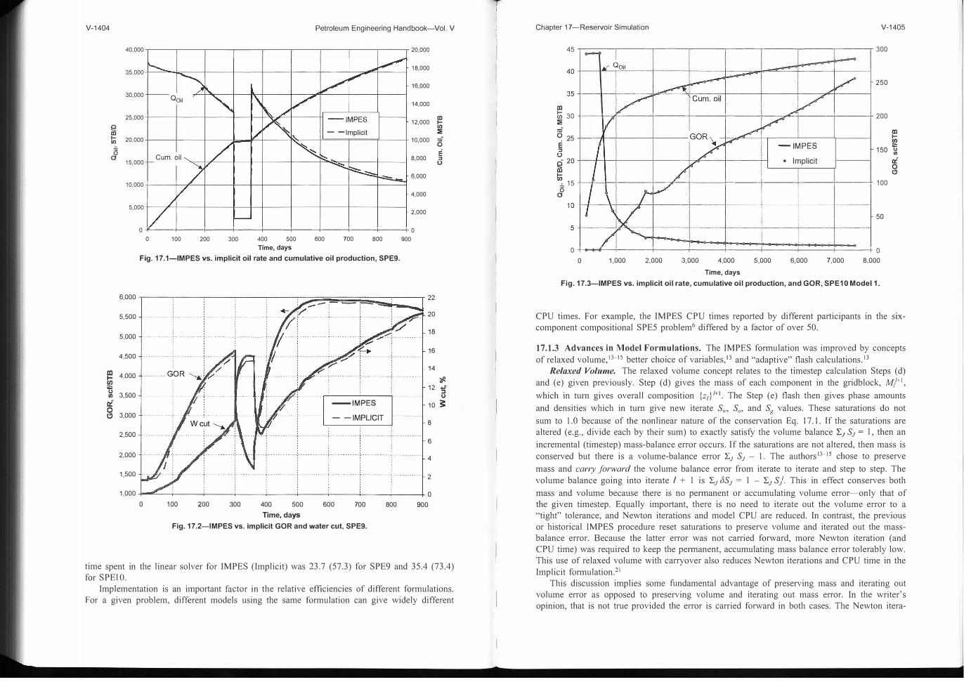
A frequently stated generalization is that numerical dispersion error is significantly larger for Implicit than for IMPES fonnulations. Truncation error analysis26 shows this error to be proportional to l,.x + uM for Implicit and l,.x - ul,.t for IMPES. Real problem nonlinearities and heterogeneity render the analysis approximate and the generalization of limited merit. For example, Figs. 17.1 through 17.3 show virtually identical Implicit and IMPES results for the blackoil 9 ,000-block SPE9 and 2,000-block gas/oil SPE 10 problems. For SPE9 (SPE 10), the average timestep was 67 (9.7) times larger for Implicit than for IMPES. The percentage of total CPU
I
V-1406 Petroleum Engineering Handbook-Vol. V
tion requirement and CPU time should be similar if "equivalent" mass and volume error tolerances are used as convergence criteria.
Variable Choice. The linear algebra required to reduce the gridblock's n conservation equations to the IMPES pressure equation is influenced by the choice of variables. The influence is absent for black oil, moderate for "moderate" n and up to a factor of three for large n (say, > 15).22 The choices of p and mo] fractions {z1}
13 or mo] numbers 14•
15 are better than the
choice of p, saturations, and phase mo] fractions 12 for large n. The effect of this variablechoice on total CPU time is often small because the affected work is often a small part of totalCPU time. This IMPES reduction is absent in the Implicit formulation and the last of theabove variable choices is arguably preferable.22
Adaptive Flash Calculations. 13 The work of EOS flash calculations, including the generation of fugacities and their derivatives, can significantly affect model efficiency when the linear solver does not dominate total CPU time. There may be little need to perform (most ot) that work in a gridblock when p and composition are changing slowly. Use of internal, intelligent criteria dictating when that work is needed can significantly reduce the total-run flash calculation CPU time. 13 This is similar in principle to the AIM selection of explicit variables for gridblocks which are quiescent in respect to throughput ratio.
17.1.4 Stable Timestep and Switching Criteria. This topic relates to the observation that lower run turnaround time can increase benefits from a reservoir study allotted a budgeted time period. As a corollary, time spent in repeated runs fighting model instabilities or time-stepping is counterproductive. While many factors affect this run time, it always equals the product (CPU time/step) x (number of timesteps). The first factor is "large" and the second "small" for the Implicit formulation, and conversely for the IMPES fonnulation. IMPES is a conditionally stable fonnulation requiring that /).t < !)./* to prevent oscillations and error growth, where !)./* is maximum stable timestep. The conditional stability stems from the explicit treatment of nonpressure variables in the interblock flow terms. Mathematicians performed stability analyses for constant-coefficient difference equations bearing some resemblance to IMPES. Authors 111 our industry extended and applied their results to derive expressions for/)./*, in particular,27
for the black-oil 30 case of gas/oil flow. This shows that stable step /)./* is dependent upon flow rates, phase mobility, and capillary pressure derivatives, which of course vary with time and from one gridblock to another. Thus, at a given timestep, there are block-dependent stable step values !).t*;, where 1 < i < N, and the IMPES stable step is Min(i) !)./*;. An IMPES model
using this internally determined stable step will run stably but may suffer from the weakestlink principle. As an extreme example, consider a 500,000-gridblock problem where, over a 100-day period, the !).t*; value is 0.01 day for one block and > 30 days for all other blocks. The
IMPES model will require 10,000 timesteps over the I 00-day period. In the AIM formulation, the stable step !).t'; depends upon the number and identities of
variables chosen explicit in block i; theoretically, !).t'; = oo if all block i variables are chosen implicit. ln the previous example, all nonpressure variables could be chosen implicit in the block where !).t
°; = 0.01 and explicit in all other blocks. The AIM model would then require
CPU time/step essentially no greater than the IMPES model but would require only three timesteps for the 100-day period.
Numerous papers28-
33 address the problem of determining expressions for the M'; for use internally as switching criteria to select block variables as explicit or implicit in the AIM
Chapter 17-Reservoir Simulation V-1407
model. The stability analyses involved are complex and may be impractically complex when allowing the implicit vs. explicit variable choice to include all permutations (in number and identity) of the n variables. The most reliable and efficient AIM models in the future will stem from continuing research leading to the following: (a) !).t*; estimates which are "accurate," and (b) implicit vs. explicit variable choices, block by block, which are near-optimal34 and minimize total CPU time, (CPU time/step) x (number of steps).
17.1.5 The Linear Solver. Preconditioned Orthomin35 is the most widely used method for iterative solution of Eqs. 17.3 or 17.7. Nested Factorization (NF)36 and incomplete LU factorization [ILU(n)]37 are the two most widely used preconditioners. The tenn "LU factorization" refers to the factoring of the matrix A into the product of a lower triangular matrix L and an upper triangular matrix U. That is an expensive operation but is straightforward, involving only Gaussian elimination. The term "ILU(n)" denotes incomplete LU factorization, where only limited fill-in is allowed and n is the "order of fill."37 NF perform� exceptionally well when transmissibilities associated with a particular direction (in a structured grid) dominate those in other directions unifonnly throughout the grid. In general, ILU(n) or red-black ILU(n)38 [RBILU (n)] is less sensitive than NF to ordering of the blocks and spatial variation of the direction of dominant transmissibilities. In addition, RBILU(n) or ILU(n) have the parameter n (order of allowed infill) which can be increased as needed to solve problems of any difficulty.
A literature search and discussions with numerous developers and users have failed to establish consensus on whether NF or ILU preconditioning is better. Some are strong advocates of one method and others are just as adamantly supportive of the other. But many find, like this writer, that the better method is problem-dependent and it is difficult to find a reliable a priori indicator for making an up-front choice. In the writer's experience, (a) when NF works well, it is faster than ILU methods, (b) RBILU(0) with no residual constraint is frequently the best of the ILU variants and a good default choice, and (c) in some cases, global residual constraint with the ILU or RBILU method is beneficial.
17.1.6 Cartesian Grids and Reservoir Definition. For many years, simulation used orthogonal Cartesian grids. In the past 15 years, numerous papers have described local grid refinement and various non-Cartesian grids, as discussed in the Gridding section. These papers show that non-Cartesian grids can reduce grid-orientation effects and provide definition and accuracy near wells, faults, highly heterogeneous areas, and so on more efficiently than Cartesian grids. The premise that Cartesian grids cannot provide required accuracy efficiently in these respects has come to be accepted as a fact. In addition, advances in geophysics have led to geostatistical description of permeability and porosity on a fine scale once unimaginable. Increasingly, our papers include examples using thousands of gridblocks for two- or few-well "patterns," in part to reflect these geostatistical descriptions. The purpose of this section is to show, using a few examples, that Cartesian grids can provide adequate accuracy and reservoir and near-well definition efficiently in some cases, even without local grid refinement. No generalizations from the examples used are intended. For the most part, the examples are taken from the literature.
SPE7 is an x-direction horizontal well problem with a 9 x 9 x 6 Cartesian grid representing a 2,700 x 2,700 x 160-ft reservoir section. The specified block !).y values decrease from 620 to 60 ft at the well, presumably to increase near-well definition and accuracy of results. The !).x
are uniformly 300 ft. Fig. 17.4 compares Case I A results for the SPE7 grid with results using unifom1 areal spacing /).x = !).y = 300 ft. The near-well y-direction refinement of the specified grid has no effect and is not necessary in this problem.
SPE8 is a gas/oil problem with one gas injector and two producers on the comers of a 5,000 x 5,000 x 325-ft square reservoir. A IO x IO x 4 Cartesian grid with uniform & = !).y = 500 ft is specified. Five participants compared their results for that grid with results from their

V-1408 Petroleum Engineering Handbook-Vol. V
lll
(/J
3,000
2,500
l;j 2,000
a
e (3 1,500
� 1,000 5
500
0
t ' L,..,--1' •
I� • Wcut \ /
\! Iv Ooil
t "" � �
i, ___.. ,__.
0 200 400
-
,� - - -
- 9x9x6 Variable Y spacing
• 9x9x6 Uniform Y spacing
Cum. oil
� .·-
. - . . - . .
600 800 1,000 1,200
Time, days
1,400
Fig. 17.4-Effect of near-well grid refinement, SPE7 Case 1A.
100
90
80
70
60 ,f!.
,____ 50 3::
40
-30
20 - .
10
1,600
11,000 -,------,---------------------------
10,000 ······-·-··-···-······-·-··-·· -·-···········-···-·········-·· ·······-······-······-···-··-··f···-···-··-·····-··-···-····-· ·-······- ·-·· -···············
9,000-+------+---• !
--1ox10x4 grid 8,000 ······························ ·······························
--sx5x4 grid
7,000 -'---------•-------------------------------·'-: ---
6,000 -�- --- --;:, - - -! .. -·(!)
5,000
4,000
3,000
2,000
!!
___ _._ :
�� ��:: :�����-�:�-- ---1=: -1,000+-------t-------t-------i------+--------l
0 500 1,000 1,500 2,000 2,500
Time,days
Fig. 17.5-Effects of coarser grids on producing GOR.
(areally) locally refined or unstructured grids. They showed good agreement for grids havingapproximately four times fewer blocks than the 10 x 10 x 4 grid. Fig. 17.5 shows equallygood agreement for a 5 x 5 x 4 (.6.x = .6.y = 1,000 ft) Cartesian grid with no local refinement.
Chapter 17-Reservoir Simulation
8,000 ---------------------------- 100
7,000 :::d....-�=::::t:::::==t 90 ------------- --------l----i----+----4!··------------1--------_:-----.'-- -------------t-------------
--�-·······!··············i
········ al 6,000
- 5-point (T)
80
70
....:: 5,000 60
V-1409
e :::i 4,000 50 :i ()
� 3,000
82,000
1,000
0
-----------1--------------t-------------·t··--· ! ! l : : :
30
20
10
l ! l .-.e........-i-------t---+---+----t---i----+---+----+---+O
0 200 400 600 800 1,000 1,200 1,400 1,600 1,800 2,000
Time, days
Fig. 17.6-9-point vs. 5-point, SPE10 Model 2.
�
SPElO (Model 1) is a 2D cross-sectional gas/oil problem with a geostatistical permeabilitydistribution given on a 100 x 1 x 20 Cartesian fine grid. Coarse-grid submittals included results using upscaling and local grid refinement. A homogeneous 5 x 1 x 5 Cartesian grid withno alteration of relative permeability matched the 100 x 1 x 20 results nearly exactly. 11
SPE 10 (Model 2) is a 3D water/oil problem with a 1.122 million-cell geostatistical grid.Some coarse grid submittals included sophisticated upscaling and gridding techniques with nopseudoization of relative penneability and grids from 4,810 to 70,224 blocks. Others used simple flow-based upscaling to 75- to 2,000-block Cartesian grids with moderate k,. changes. Ingeneral, the latter submittals showed the best agreement with the fine-grid solution. 11
Numerous papers show that non-Cartesian grids can significantly reduce the grid-orientationeffects of Cartesian grids. However, most of the examples used to study those effects are highly adverse mobility ratio displacements in homogeneous, horizontal reservoirs. In reservoirswith more nonnal fluid mobilities, areal fluid movement is more strongly affected by heterogeneity and/or gravity forces associated with reservoir structure (variable dip), and grid-orientation effects tend toward a second-order effect. As an example, the SPElO (Model 2) water/oilproblem reservoir is highly heterogeneous. Fig. 17 .6 compares five-point and nine-point fieldresults for an upscaled 28 x 55 x 85 Cartesian grid. The close agreement indicates an absenceof grid-orientation effects even though the unfavorable oil/water viscosity ratio is IO and thereis no dip.
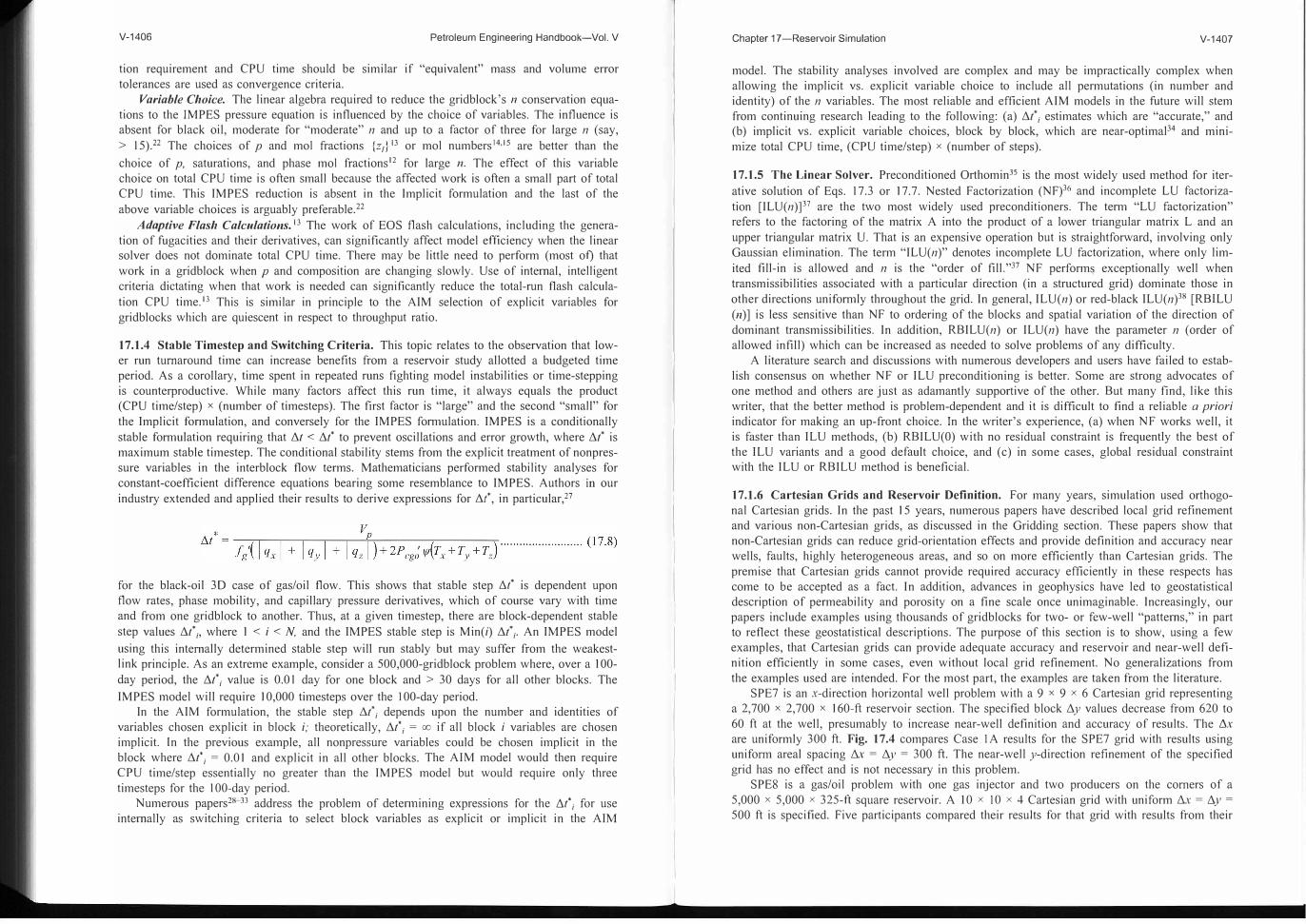
Example 17.1. Table 17 .2 gives data for Example 17. I, a ¼ five-spot, vertical-well problem. Fig. 17.7 shows two block-centered grids (a) and (b) used for this type of problem. Thefour-fold smaller well blocks of grid (b) provide finer well definition and presumably increasethe accuracy of results. Fig. 17.8 shows the identical results for IO x 10 grid (a) and 11 x 11grid (b). Results are nearly identical for the 5 x 5 grid (a) and 6 x 6 grid (b), and Fig 17.9
shows insignificant difference between 3 x 3 grid (a) and 4 x 4 grid (b) results. The grid (b)doubles the grid (a) IMPES run CPU time but contributes no greater accuracy. Well-index ef-
V-1410 Petroleum Engineering Handbook-Vol . V
TABLE 17.2-EXAMPLE 1 DATA
\ 40-acre five -spot with no dip and 180-ft pay thickness
Incompressible oil and water properties: Po = 43 lbm/ft 3 /10 = 3 cp Rs= 0
Pw = 64 lbm/ft3 /lw = 0.3 cp
Grid: N,= Nr /',.x = /',.y N,= 15/',.z=15ft
,P= 0.2 k, = 1000 md k, = 100 md
Swc= Sorw= 0.2 k,wro= 1.0 krocw = 1.0
krw= k,wro[(S.,-Swc)/(1.0-Sw -SOJ"\� )], krw<1.0
k,o = krocw[(1.0-Sw -Sorw)f(1.0-Swc -So,;)]
Water injection well at x = y = 0 is completed in all 15 layers and injects 2,550.7 STB/D water
Production well at x = y = 660 ft is completed in top 5 layers (upper 1/3 of pay) and flows on pressure constraint against a bottomhole wellbore pressure of 4,000 psia
Discussion of runs for this problem refers to various grids by their N, x Nr dimensions because N, = 15 in all cases
• • •
• • •
• • •
(a) (b) Fig. 17.7-Block-centered 3 x 3 and 4 x 4 Cartesian grids used in Example 17.1.
fects are not important here. When they are, a single one-layer single-phase run can be made
to detennine the index correction factor for grid (a) wells located in the comers of their gridblocks.
Fig. 17.10 shows a small effect of grid refinement on Example 17.1 results for grids from
20 x 20 to 3 x 3. The results indicate little need to enhance near-well definition by unstruc
tured grids or by grid refinement (global or local) for grids finer than 3 x 3 for this problem.
Example 17.2. Flexible non-Cartesian grids are shown to significantly reduce the re
quired number of gridblocks.39 An example provided40 was water/oil coning in a horizontal
well in a 600 x 300 x 230 m homogeneous reservoir. Results were: (a) a 25,823-block 31 x 17
Chapter 17-Reservoir Simulation V - 1411
3,000
80
2,500 70
I-
Cl) 2,000 �
0
E 1,500
-;f:. 50 ...
40 S:
I- 1,000 Cl)
500 __ __, -····················-· 10
o--------i-''----i------+-----+-----+----40
0 200 400 600 800 1,000 1,200
Time, days
Fig. 17.8-Effect of (a) 10 x 10 vs. (b) 11 x 11 grid on Example 17.1 results .
x 49 Cartesian grid was required to obtain a converged solution, and (b) a 3D 2,066-block
CVFE unstructured grid gave correct results. Table 17.3 gives data for Example 17.2, a similar
problem. Fig 17.11 compares Example 17.2 results for 60 x 3 I x 48 and 10 x 7 x 9 Cartesian
grids. The 630-block coarse Cartesian grid results here agree as well with the Cartesian 60 x
31 x 48 fine-grid results as the reported 2,066-block CVFE results agree with the 31 x 17 x
49 Cartesian fine-grid results.
Non-Cartesian grids are argued to define irregular reservoir boundaries more efficiently
than Cartesian grids. This is not ,necessarily true. For over 30 years, many models have used
active-block coding. While the Cartesian grid extends past boundaries to numerous inactive
blocks, those inactive blocks are dropped by the model and require no computer storage or
CPU. These numerous inactive blocks pose a problem only for models, if any, that do not use
active-block coding.
17.2 Linear Solver-John Wallis and J.W. Watts
The linear equation solver is an important component in a reservoir simulator. It is used in the
Newton step to solve the discretized nonlinear partial differential equations. These equations
describe mass balances on the individual components treated in the model. For nonisothennal
problems, an energy balance is added to the system. The matrix problem involves solving
Ax = b, where A is typically a large sparse matrix, b is the right-side vector, and x is the vec
tor of unknowns. In the IMPES fonnulation, there is a single unknown per cell pressure. In the
fully implicit fomrnlation, there is a fixed number n of unknowns per cell where n 2: 2. In the
adaptive implicit formulation, there is a variable number of unknowns per cell. In most fonnu
lations, pressure is an unknown for each cell. The matrix A typically has associated well
constraint equations and well variables and may be partitioned in block 2 x 2 fonn as

V-1412
(/)
0
in
0 0
3,000
2,500
2,000
1,500
1,000
Petroleum Engineering Handbook-Vol. V
------------------- - --------------------!--------------- - --:----------------------·�-------i:··------1I �
]
:cut
! i;---------------------- ------------ -3X3 grid (A) ----------------------
! -4X4 grid (B)
---------l---------------------1----------------------+---------------------- ----------------------
l ______________________ l_�um .�'.'. __ �---i ______________________ : ----------------------_________________ j ______________________ :---�- I --l
i-
: t
! i
90
80
70
60
50 ::,!:: "
40 :!:30
20
10
! l Of----""-!'�----1------+-----1------+----+ 0
0 200 400 600 800 1,000 1,200
Time, days
Fig_ 17.9-Effect of (a) 3 >< 3 vs_ (b) 4 >< 4 grid on Example 17.1 results.
[ A
w,v A
w,][ X"'] =[ b
bw ], -·-·-·-·-·-···-·-·-····-·-·-·-·-···-·-····--···· (17.9)A nv A,.,. XR R
where xw
is the well variable-solution vector and x R is the reservoir variable-solution vector. The matrix A
ww is often diagonal. In this case, the well variables may be directly eliminated,
and the iterative solution is on the implicitly defined matrix system
The well variables are then obtained by back substitution as
xw = A�v'./bw
- Aw
RxR) - ·-··-·--··-·-··-··-····-····-·--·--·-·······-·-··-· (17.11)
If A is large, solution of the matrix equations is impractical using direct methods such as Gaussian elimination because of computer storage or CPU time requirements. Iterative solution based on projection onto Krylov subspaces is typically used. These Krylov subspaces are spaces spanned by vectors of the fonn p(A)v, where p is a polynomial. Basically, these techniques approximateA-1 b by p(A)b_ The commonly used methods for constructing p(A)b areOrthomin36 and GMRES_41 Both methods minimize the residual norm over all vectors in span{b, A b, A2 b, - - ·, A111 -1b}at iteration m. They should yield identical results. From a practical standpoint, it does not matter which is used.
A technique known as preconditioning can improve both the efficiency (speed in a typical problem) and robustness (ability to solve a wide range of problems at least reasonably well) of Orthomin or GMR.ES_ Preconditioning involves transfom1ing the original matrix system into one with the same solution that is easier to solve. As a rule, the robustness of the iterative
Chapter 17-Reservoir Simulation V-1413
3,000
1 ---T-- -7--- -!---1--=:::;;;;;�-----7 90
80
-20x20 70
-10x10i :: .· T---,11',';,---
-------------------- 60
�- 1,500 _______________________ !_________ -------
in 1-(/)
0 0
- 5x5
- 3x3 50 'if!.
:i 40 U
:!:
20
10
o--�---,'-----+-----+-------if-----+----+o
0 200 400 600 800 1,000
Time, days Fig. 17-10-Effects of Cartesian grid coarsening, Example 17_ 1 results_
TABLE 17.3-EXAMPLE 2 DATA
Water/oil coning problem with a 300-m x-direclion horizontal well Reservoir dimensions: 600X300X230 m Pay zone thickness: 35 m Aquifer thickness: 195 m Producer: x = 150 m to 450 m, y = 150 m, z = 10 m, rate = 1,315 STB/D liquid Water injector: x = 300 m, y = 150 m, z = 140 m, rate = 1,315 STB/D water
k,= ky= 360 md k, = 60 md t/J= 0.21
Incompressible water and oil, B0 = B,., = 1 _0 RB/STB, Rs
= 0 Po
= 53.04 lbm/ft3 Po= 1.2 cp
Pw = 64.27 lbm/fl3 flw= 0.52 cp
knvro= 0.22 kroew= 1.0 Swe= 0.296 Sonv= 0.31
krw = k,wroS,.,,,2 (krw< 1) kro = krocwSo/ Pewo
= 2.4*[(1.0-Sw)/(1.0-Sw/)] psi Water/oil contact at z = 35 m (Pewo
= 0)
1,200
scheme is far more dependent on the preconditioning than on the specific Krylov subspace accelerator used. The preconditioner M is a matrix that approximates A, and has the property that the linear systems of the fonn Mx = b are easily and inexpensively solved. For most linear solvers the following preconditioned system is solved:
-I -I AM y = b, where x = M y _
V-1414 Petroleum Engineering Handbook-Vol. V
1400 45
40 1200
35
� 1000 30
i5 E 800 25 :,g " ::i
0
ci 600 20 3:
15 0 400 a
10
200 5
0 0 0 100 200 300 400 500 600 700 800 900 1,000
Time, days
Fig. 17.11-Fine vs. coarse Cartesian grids, Example 17.2.
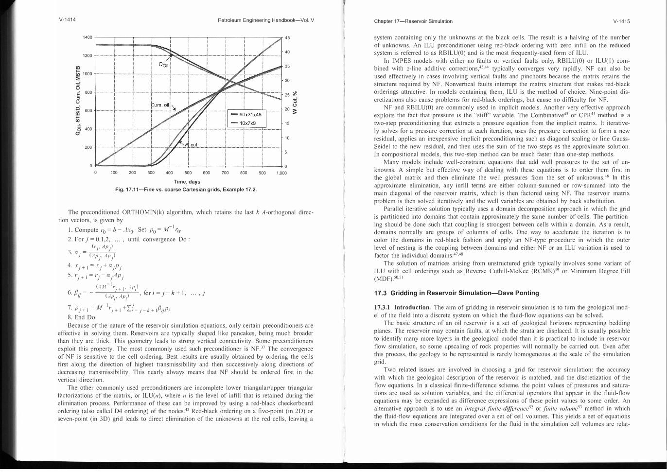
The preconditioned ORTHOMIN(k) algorithm, which retains the last k A-orthogonal direction vectors, is given by
1. Compute r0 = b - Ax0. Set p0 = M-1 r0.2. For j = 0, 1,2, ... , until convergence Do :
(r ., Ap .) 3 a = .I .I . J (Ap
j' Ap}
4. xJ+l =x1 +a1p1
5. rJ+l =r1-a1Ap1
( -I AM r. + 1,Ap.)
6 (J .1 1 fi · · /, I . ij
= -(A A ) ' or I = J - C + ' ... ' jp
i' P;
7. Pj+l =M-',-j+l +I(= J-k+lfJijPi
8. End Do Because of the nature of the reservoir simulation equations, only certain preconditioners are
effective in solving them. Reservoirs are typically shaped like pancakes, being much broader than they are thick. This geometry leads to strong vertical connectivity. Some preconditioners exploit this property. The most commonly used such preconditioner is NF.37 The convergence of NF is sensitive to the cell ordering. Best results are usually obtained by ordering the cells first along the direction of highest transmissibility and then successively along directions of decreasing transmissibility. This nearly always means that NF should be ordered first in the vertical direction.
T�e �ther commonly used preconditioners are incomplete lower triangular/upper triangularfa�t�nz�t1ons of the matrix, or ILU(n), where n is the level of infill that is retained during theehmmation process. Perfonnance of these can be improved by using a red-black checkerboard ordering (also called D4 ordering) of the nodes.42 Red-black ordering on a five-point (in 2D) or seven-point (in 3D) grid leads to direct elimination of the unknowns at the red cells, leaving a
Chapter 17-Reservoir Simulation V-1415
system containing only the unknowns at the black cells. The result is a halving of the number of unknowns. An ILU preconditioner using red-black ordering with zero infill on the reduced system is referred to as RBILU(0) and is the most frequently-used form of ILU.
In IMP ES models with either no faults or vertical faults only, RBILU(0) or ILU( I) combined with z-line additive corrections,43
•44 typically converges very rapidly. NF can also be
used effectively in cases involving vertical faults and pinchouts because the matrix retains the structure required by NF. Nonvertical faults interrupt the matrix structure that makes red-black orderings attractive. In models containing them, ILU is the method of choice. Nine-point discretizations also cause problems for red-black orderings, but cause no difficulty for NF.
NF and RBILU(0) are commonly used in implicit models. Another very effective approachexploits the fact that pressure is the "stiff' variable. The Combinative45 or CPR44 method is atwo-step preconditioning that extracts a pressure equation from the implicit matrix. It iteratively solves for a pressure correction at each iteration, uses the pressure c01Tection to form a new residual, applies an inexpensive implicit preconditioning such as diagonal scaling or line GaussSeidel to the new residual, and then uses the sum of the two steps as the approximate solution. In compositional models, this two-step method can be much faster than one-step methods.
Many models include well-constraint equations that add well pressures to the set of unknowns. A simple but effective way of dealing with these equations is to order them first in the global matrix and then eliminate the well pressures from the set of unknowns.46 In this approximate elimination, any infill tenns are either column-summed or row-summed into the main diagonal of the reservoir matrix, which is then factored using NF. The reservoir matrix problem is then solved iteratively and the well variables are obtained by back substitution.
Parallel iterative solution typically uses a domain decomposition approach in which the grid is partitioned into domains that contain approximately the same number of cells. The partitioning should be done such that coupling is strongest between cells within a domain. As a result, domains nonnally are groups of columns of cells. One way to accelerate the iteration is to color the domains in red-black fashion and apply an NF-type procedure in which the outer level of nesting is the coupling between domains and either NF or an ILU variation is used to factor the individual domains.47,48
The solution of matrices arising from unstructured grids typically involves some variant of ILU with cell orderings such as ,Reverse Cuthill-McKee (RCMK)49 or Minimum Degree Fill (MDF)_so,s ,
17.3 Gridding in Reservoir Simulation-Dave Ponting
17.3.1 Introduction. The aim of gridding in reservoir simulation is to turn the geological model of the field into a discrete system on which the fluid-flow equations can be solved.
The basic structure of an oil reservoir is a set of geological horizons representing bedding planes. The reservoir may contain faults, at which the strata are displaced. It is usually possible to identify many more layers in the geological model than it is practical to include in reservoir flow simulation, so some upscaling of rock properties will normally be carried out. Even after this process, the geology to be represented is rarely homogeneous at the scale of the simulation grid.
Two related issues are involved in choosing a grid for reservoir simulation: the accuracy with which the geological description of the reservoir is matched, and the discretization of the flow equations. In a classical finite-difference scheme, the point values of pressures and saturations are used as solution variables, and the differential operators that appear in the fluid-flow equations may be expanded as difference expressions of these point values to some order. An alternative approach is to use an integral jinite-dijference52 or finite-volume53 method in which the fluid-flow equations are integrated over a set of cell volumes. This yields a set of equations in which the mass conservation conditions for the fluid in the simulation cell volumes are relat-
V-1416 Petroleum Engineering Handbook-Vol. V
ed to the flows through the interfaces between those cell volumes. Rock properties such as porosity are assumed constant over the cell or controlled volume. This yields a discretization scheme which is conservative ( each outflow from one cell is an inflow to another) and for which the fluid in place may be obtained straightforwardly. The mass conservation equations for a timestep from T to T + t,,T then become:
T+/',.T T+t,_T T T ( '°' '°' ) Vpa ·mca -Vpa ·mca = t,,T • Qca
+ L.bL. pFc
pab, ···························· (17.!2)
where �'" is the pore volume of cell a, mca
is the density of conserved component c in cell a,Qca is the injection or production rate of component c because of wells, and F,pab is the flow rate of component c in phase p from cell a to its neighbor b. In general, the flows F,
pab may involve the solution values of a number of cells, the number of cells involved defining the stencil of the numerical scheme. The linear pressure dependence of flows given by Darcy's law leads to an expression of the type:
Fcpab =IxTax�
paxt,,<l>pax · ················································· (17.13)
�pax is the mobility of component c in phase p for the contribution to the flow between a and x, given by x
c,,.K,p /p
p, where xcp
is the concentration of component c in phase p, K,p is the relative pem1eability of phase p, and /I
p is the viscosity of phase p. This is often set to an
upstream value of the mobility, depending upon the sign of the potential difference. t,,<l>p,u is the potential difference of phase p between cell a and cell x, which includes pres
sure, gravity and capillary pressure contributions:
t,_q> pax = pa -px -gp p • (da - d) + p cpa -p cpx · · · · · · · · · · · · · · · · · · · · · · · · · · · · · · · · (17 .14)
The constant coefficients of mobility and potential difference products, Ta.n are commonly termed the transmissibi/ities.
When the flows between two cells a and b can be expressed as a function of the solution values in just those two cells, so that the summation over cells includes just x = b, the flow expression takes a two-point fonn. The flow expression then takes a simple form:
Fcpab = Tap�
pabt,,<l> pab · ··········· ········································ (17 .15)
When solution values from other cells are required, the flow takes a multipoint form.54
Other options for discretization are available, such as Galerkin finite elements55-57 and mixed finite-element.58 It is sometimes possible to cast a finite-element Galerkin discretization into the upstreamed transmissibility-based form.57
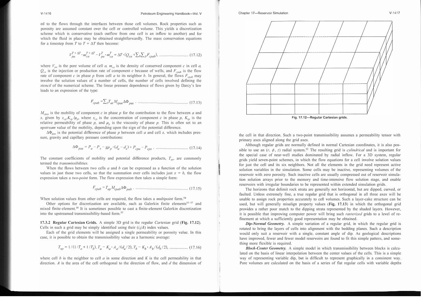
I 7.3.2 Regular Cartesian Grids. A simple 3D grid is the regular Cartesian grid (Fig. I 7.12).
Cells in such a grid may be simply identified using their (i,j,k) index values. Each of the grid elements will be assigned a single permeability or porosity value. In this
case, it is possible to obtain the transmissibility value as a harmonic average:
where cell b is the neighbor to cell a in some direction and K is the cell pem1eability in that direction. A is the area of the cell orthogonal to the direction of flow, and d the dimension of
T Chapter 17-Reservoir Simulation V-1417
Fig. 17.12-Regular Cartesian grids.
the cell in that direction. Such a two-point transmissibility assumes a permeability tensor with primary axes aligned along the grid axes.
Although regular grids are normally defined in normal Cartesian coordinates, it is also possible to use an (r, ¢, z) radial system.52 The resulting grid is cylindrical and is important forthe special case of near-well studies dominated by radial inflow. For a 30 system, regular grids yield seven-point schemes, in which the flow equations for a cell involve solution values for just the cell and its six neighbors. Not all the elements in the grid need represent active solution variables in the simulation. Some cells may be inactive, representing volumes of the reservoir with zero porosity. Such inactive cells are usually compressed out of reservoir simulation solution arrays prior to the memory and time-intensive flow solution stage, and enable reservoirs with irregular boundaries to be represented within extended simulation grids.
The horizons that delimit rock strata are generally not horizontal, but are dipped, curved, or faulted. Unless extremely fine, a true regular grid that is orthogonal in all three axes will be unable to assign rock properties accurately to cell volumes. Such a layer-cake structure can be used, but will generally misalign propetiy values (Fig. 17.13) in which the orthogonal grid provides a rather poor match to the dipping strata represented by the shaded layers. However, it is possible that improving computer power will bring such rasterized grids to a level of refinement at which a sufficiently good representation may be obtained.
Dip-Normal Geometry. A simple variation of a regular grid, in which the regular grid is rotated to bring the layers of cells into alignment with the bedding planes. Such a description would only suit a reservoir with a single, constant angle of dip. As geological descriptions have improved, fewer and fewer model reservoirs are found to fit this simple pattern, and something more flexible is required.
Block-Center Geomefly. A simple model in which transmissibility between blocks is calculated on the basis of linear interpolation between the center values of the cells. This is a simple way of representing variable dip, but is difficult to represent graphically in a consistent way. Pore volumes are calculated on the basis of a series of flat regular cells with variable depths

V-1418 Petroleum Engineering Handbook-Vol. V
Fig. 17.13-0rthogonal grid used to represent dip.
I
Fig. 17.14-(a) Obtaining pore volumes; (b) obtaining transmissibilities.
(Fig. 17.14a), but transmissibilities are calculated on the basis of interpolated values (Fig.
17.14b). The areal grid is rectangular.
Thus, for the pair of cells illustrated,
T = K · A Id, where KI d = 2 I (d1 I K1 + d2 I K
2), ................................ ( 17. 17)
where A is the average area over which flow occurs and c is a dip correction given by cos20, where 0 is the angle of dip of a line joining the cell centers to the horizontal. Such a block
center option is suitable for unfaulted reservoirs and is commonly supplied as a simulator option.
17.3.3 Hexahedral Grids. Further improvements in geological modeling threw an emphasis
on describing faults, and made it important to distinguish depth displacements due to dip and
faulting. This is difficult in block centre geometry in which the cell is positioned by its centre
depth and fix, Liy, Liz dimensions. To define faulting more precisely it is useful to define the
position of grid cell by its corner point locations. A hexahedral shape with eight corners and
Chapter 17-Reservoir Simulation V-1419
Fig. 17.15-Hexahedral grid system.
bilinear planes as surfaces then describes the cell geometry. Faults, both vertical and inclined,
may be described precisely (Fig. 17.15). Such grids are often called corner-point grids.
In both the dipped and general hexahedral grids, the orthogonality of a completely rectangu
lar grid no longer exists, and the result is that the two-point property of the flows between the cells is lost-the flow between cell a and cell b is not just a function of the solution values of
cells and a and b.53•59
-62 Typically, the result is a 27-point scheme in three dimensions. Howev
er, if the grid distortion is mild, it may be possible to ignore some additional couplings and
use a low-order transmissibility scheme. This is normally done for extra couplings introduced
by dip angles, which are often small.
Although this corner-point description handles the fault issue, the basic coordinate system
remains a regular grid (i.e., the grid is structured). Fitting such a basically regular system to
the irregular shapes of a reservoir remains a difficulty that may be solved in two basic ways
either by distorting the grid and fitting the cells into the geometry, or by truncating the grid to
the reservoir position.
17.3.4 Multiple-Domain Hexahedral Grids. In some cases, a single structured grid system
cannot match the overall structure of a reservoir, so a block grid or domain-based grid is
used.63 This consists of a number of subgrids, each with a local regular (i.j,k) structure, but
linked together to model the entire reservoir. The block hexahedral system gives rise to multi
ple (i.j,k) indexing systems-(i.j,k,/), where the I index specifies the grid system. These
comprise a series of regular grids. Such regular gridding systems have advantages for upscaling
and downscaling-for example, a natural coarsening of a regular grid may be simply defined
by grouping sets of coordinates in each direction.
17.3.5 Grid Refinement. A common requirement in reservoir simulation is an increased level
of detail around an item of interest such as a well. This is frequently obtained in structured
grids by local grid refinement, replacing a set of cells in the original grid by a finer grid (Fig.
17.16). The inserted grid may be Cartesian ( center) or radial (upper left). Local refinement may be regarded as a form of multiple domain structured grid, in that it consists of a number of
linked structured grids. Flows at the edges of local refinements generally take a multipoint
form.54
17.3.6 Unstructured Grids. The problems involved in using a regular structured grid to repre
sent reservoir geometry can be avoided by using an unstructured grid. This is constructed around a set of solution points that need have no particular indexing scheme. These points may
V-1420 Petroleum Engineering Handbook-Vol. V
@
Fig. 17.16-Local grid refinement.
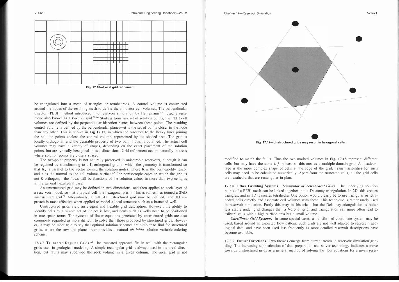
be triangulated into a mesh of triangles or tetrahedrons. A control volume is constructed
around the nodes of the resulting mesh to define the simulator cell volumes. The perpendicular
bisector (PEBI) method introduced into reservoir simulation by Heinemann64•65 used a tech
nique also known as a Voronoi grid.58•66 Starting from any set of solution points, the PEBI cell
volumes are defined by the perpendicular bisection planes between these points. The resulting
control volume is defined by the perpendicular planes-it is the set of points closer to the node
than any other. This is shown in Fig 17.17, in which the bisectors to the heavy lines joining
the solution points enclose the control volume, represented by the shaded area. The grid is
locally orthogonal, and the desirable property of two point flows is obtained. The actual cell
volumes may have a variety of shapes, depending on the exact placement of the solution
points, but are typically hexagonal in two dimensions. Grid refinement occurs naturally in areas
where solution points are closely spaced.
The two-point property is not naturally preserved in anisotropic reservoirs, although it can
be regained by transforming to a K-orthogonal grid in which the geometry is transformed so
that K" is parallel to the vector joining the solution nodes, where K is the pem1eability tensor
and n is the normal to the cell volume surface.67 For nonisotropic cases in which the grid is
not K-orthogonal, the flows will be functions of the solution values in more than two cells as
in the general hexahedral case.
An unstructured grid may be defined in two dimensions, and then applied to each layer of
a reservoir model, so that a typical cell is a hexagonal prism. This is sometimes te1111ed a 2½D
unstructured grid.68 Alternatively, a full 30 unstructured grid may be defined. The 3D ap
proach is most effective when applied to model a local structure such as a branched well.
Unstructured grids yield an elegant and flexible grid description. However, the ability to
identify cells by a simple set of indices is lost, and items such as wells need to be positioned
in true space tem1s. The systems of linear equations generated by unstructured grids are also
commonly regarded as more difficult to solve than those produced by structured grids. Howev
er, it may be more true to say that optimal solution schemes are simpler to find for structured
grids, where the row and plane order provides a natural ab initio solution variable-ordering
scheme.
17.3.7 Truncated Regular Grids. 69 The truncated approach fits in well with the rectangular
grids used in geological modeling. A simple rectangular grid is always used in the areal direc
tion, but faults may subdivide the rock volume in a given column. The areal grid is not
Chapter 17-Reservoir Simulation V-1421
•
•
•
• \ •
•
• Fig. 17.17-Unstructured grids may result in hexagonal cells.
modified to match the faults. Thus the two marked volumes in Fig. 17.18 represent different
cells, but may have the same i, j indices, so this creates a multiple-domain grid. A disadvan
tage is the more complex shape of cells at the edge of the grid. Transmissibilities for such
cells may need to be calculated numerically. Apart from the truncated cells, all the grid cells
are hexahedra that are rectangular in plan.
17.3.8 Other Gridding Systems. Triangular or Tetrahedral Grids. The underlying solution
points of a PEBI mesh can be linked together into a Delaunay triangulation. In 2D, this creates
triangles, and in 3D it creates tetrahedra. One option would clearly be to use triangular or tetra
hedral cells directly and associate cell volumes with these. This technique is rather rarely used
in reservoir simulation. Partly this may be historical, but the Delaunay triangulation is rather
less stable under grid changes than a Voronoi grid, and triangulation can more often lead to
"sliver" cells with a high surface area but a small volume.
Curvilinear Grid Systems. ln some special cases, a transformed coordinate system may be
used, based around an expected flow pattern. Such grids are not well adapted to represent geo
logical data, and have been used less frequently as more detailed reservoir descriptions have
become available.
17.3.9 Future Directions. Two themes emerge from current trends in reservoir simulation grid
ding. The increasing sophistication of data preparation and solver technology indicates a move
towards unstructured grids as a general method of solving the flow equations for a given reser-
V-1422 Petroleum Engineering Handbook-Vol. V
.
'
\
\ �
�'
I\� '
Fig. 17.18-A fault creating two cell volumes in a truncated grid.
voir simulation problem. On the other hand, reservoir simulation is increasingly seen as part of a decision-making process rather than an isolated activity, so the ability to map easily onto the generally regular data structures used in seismic and geological modeling becomes an important issue. In this role, structured grids may have advantages of simplicity and scalability.
An ideal is to separate the construction of the flow-simulation grid from the description of the reservoir geometry. This ties in with a further ideal, inherent in many discretization schemes, that the scale of the simulation grid should be below the scale of the problem structure.
For more complex shape-dominated problems, the unstructured approach looks general and flexible, providing that the data-handling and cell-identification methods can be moved to true x,y,z space preprocessing software.
17.4 Upscaling of Grid Properties-Alan Grindheim
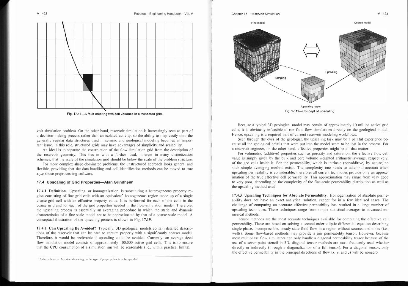
17.4.1 Definition. Upscaling, or homogenization, is substituting a heterogeneous property region consisting of fine grid cells with an equivalent* homogeneous region made up of a single coarse-grid cell with an effective property value. It is performed for each of the cells in the coarse grid and for each of the grid properties needed in the flow-simulation model. Therefore, the upscaling process is essentially an averaging procedure in which the static and dynamic characteristics of a fine-scale model are to be approximated by that of a coarse-scale model. A conceptual illustration of the upscaling process is shown in Fig. 17.19.
17.4.2 Can Upscaling Be Avoided? Typically, 3D geological models contain detailed descriptions of the reservoir that can be hard to capture properly with a significantly coarser model. Therefore, it would be preferable if upscaling could be avoided. Currently, an average-sized flow simulation model consists of approximately I 00,000 active grid cells. This is to ensure that the CPU consumption of a simulation run will be reasonable (i.e., within practical limits).
• Either volume or llux vice. depending on the type of property that is to be upscaled.
Chapter 17-Reservoir Simulation V-1423
Fine model Coarse model
Upscaling region
Fig. 17.19-Concept of upscaling.
Because a typical 3D geological model may consist of approximately IO million active grid cells, it is obviously infeasible to run fluid-flow simulations directly on the geological model. Hence, upscaling is a required part of current reservoir modeling workflows.
Seen through the eyes of the geologist, the upscaling task may be a painful experience because all the geological details that were put into the model seem to be lost in the process. For a reservoir engineer, on the other hand, effective properties might be all that matter.
For volumetric (additive) properties such as porosity and saturation, the effective flow-cell value is simply given by the bulk and pore volume weighted arithmetic average, respectively, of the geo cells inside it. For the pem1eability, which is intrinsic (nonadditive) by nature, no such simple averaging method exists. The complexity one needs to take into account when upscaling permeability is considerable; therefore, all current techniques provide only an approximation of the true effective cell permeability. This approximation may range from very good to very poor, depending on the complexity of the fine-scale permeability distribution as well as the upscaling method used.
17.4.3 Upscaling Techniques for Absolute Permeability. Homogenization of absolute permeability does not have an exact analytical solution, except for in a few idealized cases. The challenge of computing an accurate effective permeability has resulted in a large number of upscaling techniques. These techniques range from simple statistical averages to advanced numerical methods.
Tensor methods are the most accurate techniques available for computing the effective cell permeability. These are based on solving a second-order elliptic differential equation describing single-phase, incompressible, steady-state fluid flow in a region without sources and sinks (i.e., wells). Some flow-based methods may provide a .fii/1 permeability tensor. However, because most multiphase flow simulators can only handle a diagonal permeability tensor because of the use of a seven-point stencil in 3D, diagonal tensor methods are most frequently used whether directly or indirectly (through a diagonalization of a full tensor). For a diagonal tensor, only the effective permeability in the principal directions of flow (x, y, and z) will be nonzero.

V-1424 Petroleum Engineering Handbook-Vol. V
Local upscaling
Regional upscaling
Global upscaling
•
C
Fig. 17.20-Upscaling schemes and the size of the computational region (geo grid in white, flow grid in black).
The flow equation is usually discretized with a finite-difference scheme, although finite-ele
ment methods are also applied occasionally. To compute all the directional components of the
permeability tensor, the discretization and solution of the flow equation must be performed for
each of the principal flow directions (i.e., three separate single-phase simulations need to be
performed). Each simulation involves the iterative solution of a linear equation system (typical
ly, the linear solver is a conjugate gradient method, preconditioned by incomplete Cholesky or
LU factorization). The unknowns in this equation system are the geo-cell pressures inside the
flow cell, whereas known quantities are the geo-cell dimensions and permeabilities, as well as
the pressure conditions along the faces of the flow cell. When the numerical solution of the fine
scale pressure distribution has converged, an effective permeability is computed by equating
expressions for the flux through the heterogeneous geo cells with the flux through the equiva
lent homogeneous flow cell using some form of Darcy's law.
The pressure field is usually solved locally-that is, for one flow cell at a time. However,
as discussed in the next subsection, the size of the computational region may not necessarily
be limited to that of the upscaling region (i.e., the flow cell).
17.4.4 Upscaling Schemes for Absolute Permeability. Based on the size of the computational
region, the single-phase upscaling process may either be described as local, regional, or global.
With local upscaling techniques, the computational region is identical to the upscaling region
(i.e., only geo cells inside the flow cell are considered in the upscaling computations). For
regional upscaling, the computational region is expanded beyond that of the flow cell to in
clude a buffer region of neighboring geo cells. In the case of global upscaling, the computation
al region is that of the entire geo model. Fig. 17.20 provides a schematic drawing of how the
computational region varies with the different upscaling schemes. These are further discussed
in the subsections that follow.
Chapter 17-Reservoir Simulation V-1425
P=O@outlet
No flow No flow
Fig. 17.21-The sealed sides boundary conditions (in z-direction) .
It should be noted that the different upscaling schemes are only relevant when considering
flow-based (tensor) methods. It is also important to realize that even though the computational
region may vary according to the scheme used, the upscaling region remains unchanged and is
of course defined by the flow cell, as in the case of the simple, analytical upscaling techniques.
J 7.4.5 Local Upscaling. Because it used to be too time-consuming to compute the fine-scale
pressure field for the complete geo grid in a single operation, the flow-based methods have
traditionally been restricted to solving the pressure field locally-that is, for a single flow cell
at a time. Hence, the effective cell permeability is computed separately and independently of
the other flow cells, which may or may not be correct depending on how representative the
imposed pressure conditions along the faces of the flow cell are.
Different types of artificial boundary conditions for the flow cell have been suggested over
the years, all with the objective of providing as good an approximation of the real boundary
conditions as possible. An important design criterion for the artificial boundary conditions is
the conservation of flux in and out of the flow cell.
The first type of boundary conditions proposed for the local solution of the pressure equa
tion was published by Warren and Price in 1961.70 Their approach is to impose a constant
pressure gradient in a selected direction of flow by specifying a pressure of I on the _inflow
face and a pressure of O on the outflow face. By allowing no flow to pass through the sides of
the cell, all fluxes are forced to go in the principal direction of flow. Therefore, this type of
boundary conditions is often referred to as the no-flow or sealed-sides boundary conditions.
The sealed-sides boundary conditions are graphically illustrated in Fig. 17.21 for flow in the
vertical direction (here in the case of a flow cell containing a barrier).
The choice of boundary conditions emulates the way core permeability is measured in the
lab. This is hardly a coincidence. As in the coreflood experiment, the local numerical flow
simulation is in effect ID because the cell faces parallel to the main flow direction are sealed.
This implies that the estimated effective permeability will be scalar. Hence, the maximum mun
ber of directional permeability components that can be obtained with this type of boundary
conditions is three, one for each of the principal directions of flow. In practice, the diagonal
V-1404 Petroleum Engineering Handbook-Vol. V
40,000 20,000
35,000 18,000
16,000
30,000 QOil
14,000
25,000
20,000 ti)
- -Implicit
aJ 12,000
10,000 i5
0 Cum. oil 15,000
E 8,000
6,000
10,000
4,000
5,000 2,000
0+----+---+----1------1---+----+----+----+-----+ 0
0 100 200 300 400 500 600 700 800 900
Time, days
Fig. 17.1-IMPES vs. implicit oil rate and cumulative oil production, SPE9.
6,000 22
5,500 20
5,000 18
16 4,500
m 4,000
i3 3,500 Ill
14
� 0
12
-IMPES 10 s:
3,000 - -IMPLICIT8
2,500 6
2,000 4
1,500 2
1,000 0
0 100 200 300 400 500 600 700 800 900
Time,days
Fig. 17.2-IMPES vs. implicit GOR and water cut, SPE9.
time spent in the linear solver for IMPES (Implicit) was 23.7 (57.3) for SPE9 and 35.4 (73.4) for SPElO.
Implementation is an important factor in the relative efficiencies of different formulations. For a given problem, different models using the same formulation can give widely different
T Chapter 17-Reservoir Simulation V-1405
45 �--�---�---�---�--�---�---�--� 300
40 250
� 30 +----t--...,l------+----+-----1------+-�--- +------+-----+ 200
aJ II/) .;::
0 25 E -IMPES 150 �
� 20 • Implicit
..:.15+---+---t---<�---+-----+-- - -t-----+----+-----l-----+-100 0
0
50
0+-t.,...+----li----+---+----1----+---+----+-----+0
0 1,000 2,000 3,000 4,000 5,000 6,000 7,000 8,000
Time, days
Fig. 17.3-IMPES vs. implicit oil rate, cumulative oil production, and GOR, SPE10 Model 1.
ci 0 (!)
CPU times. For example, the IMPES CPU times reported by different participants in the sixcomponent compositional SPE5 problem6 differed by a factor of over 50.
17.1.3 Advances in Model Formulations. The IMPES fonnulation was improved by concepts of relaxed volume, 13-15 better choice of variables, 13 and "adaptive" flash calculations.13
Relaxed Volume. The relaxed volume concept relates to the timestep calculation Steps (d) and (e) given previously. Step (d) gives the mass of each component in the gridblock, M/+ 1
,
which in tum gives overall composition {z1}1+1• The Step (e) flash then gives phase amounts
and densities which in tum give new iterate Sw, S0
, and Sg values. These saturations do not
sum to 1.0 because of the nonlinear nature of the conservation Eq. 17.1. lf the saturations are altered ( e.g., divide each by their sum) to exactly satisfy the volume balance :EJ SJ = I, then an
incremental (timestep) mass-balance error occurs. If the sah1rations are not altered, then mass is conserved but there is a volume-balance error LJ SJ - 1. The authors13-15 chose to preserve
mass and cany forward the volume balance error from iterate to iterate and step to step. The volume balance going into iterate I + I is :EJ JSJ = I - :EJ Sj. This in effect conserves both
mass and volume because there is no pennanent or accumulating volume error-only that of the given timestep. Equally important, there is no need to iterate out the volume error to a "tight" tolerance, and Newton iterations and model CPU are reduced. In contrast, the previous or historical IMPES procedure reset saturations to preserve volume and iterated out the massbalance error. Because the latter error was not carried forward, more Newton iteration (and CPU time) was required to keep the pennanent, accumulating mass balance error tolerably low. This use of relaxed volume with carryover also reduces Newton iterations and CPU time in the Implicit formulation.21
This discussion implies some fundamental advantage of preserving mass and iterating out volume error as opposed to preserving volume and iterating out mass error. In the writer's opinion, that is not true provided the error is carried forward in both cases. The Newton itera-

V-1426 Petroleum Engineering Handbook-Vol. V
I_JI - - - -
1,-. - - -
- - - -II
1'7�1 - - -
Fig. 17.22-The fine-scale permeabilities are symmetric on the scale of the flow cell (geo grid in white, flow grid in black).
permeability tensor is derived by setting up the boundary conditions for x, y, and z directions,
respectively, in three independent single-phase simulations.
As documented in Refs. 71 and 72, a tensor technique based on the sealed-sides boundary
conditions tends to bias the estimated effective permeability toward a low value. The physical
implication of this is most clearly seen in the case of a bimodal permeability system of sand
and shale. This is because the sealed-sides method consistently underestimates the reservoir flow characteristics by thickening shale barriers and narrowing sand channels. The latter effect
also has a tendency of disconnecting stacked sand channels.
Take, for example, the flow illustrated by Fig. 17.21. Because the barrier extends across the entire length of the local upscaling region, the resulting effective permeability (in the z-direc
tion) will be zero. For vertical flow, the result, therefore, is a thickening of the shale in the
flow model equal to the thickness of the flow cell. Depending on which factors that affect
fluid flow in the region of the cell, this may or may not be a representative value for that
particular flow cell.
Strictly speaking, the sealed-sides boundary conditions are only valid if no wells are
present and the flow cells are symmetric in each direction of the grid as illustrated in 20 by
Fig. 17.22. Hence, the sealed-sides boundary conditions assume that the flow cell is surrounded
by mirror images of itself.
By the end of the 1980s, 30 geological models had started to appear more regularly on the
modeling scene. This resulted in a new demand for advanced upscaling. In this renewed effort,
two alternative boundary conditions for solving the local pressure solution in a flow-based
method were suggested more or less at the same time. One was based on linear boundary con
ditions, the other on periodic boundary conditions.
The use of linear boundary conditions in flow-based upscaling was suggested by Guerillot
et al. 73 in 1989 and Samier74 in 1990 to enable the computation of a full-permeability tensor.
Instead of setting the flow through the sides of the cell to zero, the pressure along the sides is
Chapter 17-Reservoir Simulation
P=f(z)
P=O@outlet
. ' Barrier ' ' , • r
. - . - . -
Fig. 17.23-The open sides boundary conditions (in z-direction).
V-1427
P=f(z)
allowed to vary in a linear fashion that matches the constant pressure on the two cell faces
perpendicular to the flow. Hence, the imposed pressure gradient is still constant, but the flow
is allowed to enter and leave the cell at any point along the sides parallel to the main flow
direction. Therefore, this type of boundary conditions is also referred to as the open-sides bound
ary conditions. The situation is graphically illustrated in Fig. 17.23 for flow in the vertical
direction (here in the case of a flow cell containing a barrier).
As with the sealed-sides boundary conditions, three independent single-phase simulations,
with the main flow direction in x, y, and z, respectively, are needed to yield all of the compo
nents of the permeability tensor. With open-sides boundary conditions, however, also the off
diagonal components will generally be nonzero. Hence, unlike the sealed-sides boundary
conditions where the effective permeability is limited to that of a diagonal tensor, the open
sides boundary conditions, as previously mentioned, give a full permeability tensor. The
resulting full tensor may be either symmetric or nonsymmetric depending on the properties of
the method under consideration.
As documented in Refs. 75 and 76, a tensor technique based on the open-sides boundary
conditions tends to bias the estimated effective permeability toward a high value. The physical
implication of this is most clearly seen in the case of a bimodal permeability system of sand
and shale. This is because the open-sides method consistently overestimates the reservoir flow
characteristics by narrowing shale barriers and thickening sand channels. The latter effect also
has a tendency of connecting i -solated sand channels.
Take, for example, the situation illustrated by Fig. 17.23. Even though the barrier extends
across the entire length of the local upscaling region, the resulting e ffective permeability (in
the z-direction) will be significantly larger than zero. For vertical flow, the result is there fore a
narrowing of the shale in the flow model equal to the horizontal dimensions of the flow cell.
Depending on which factors affect fluid flow in the region of the cell, this may or may not be
a representative value for that particular flow cell.
The use of linear boundary conditions has its origin in the effective medium theory,77
which states that any region of permeability behaves as if embedded within the average medi-
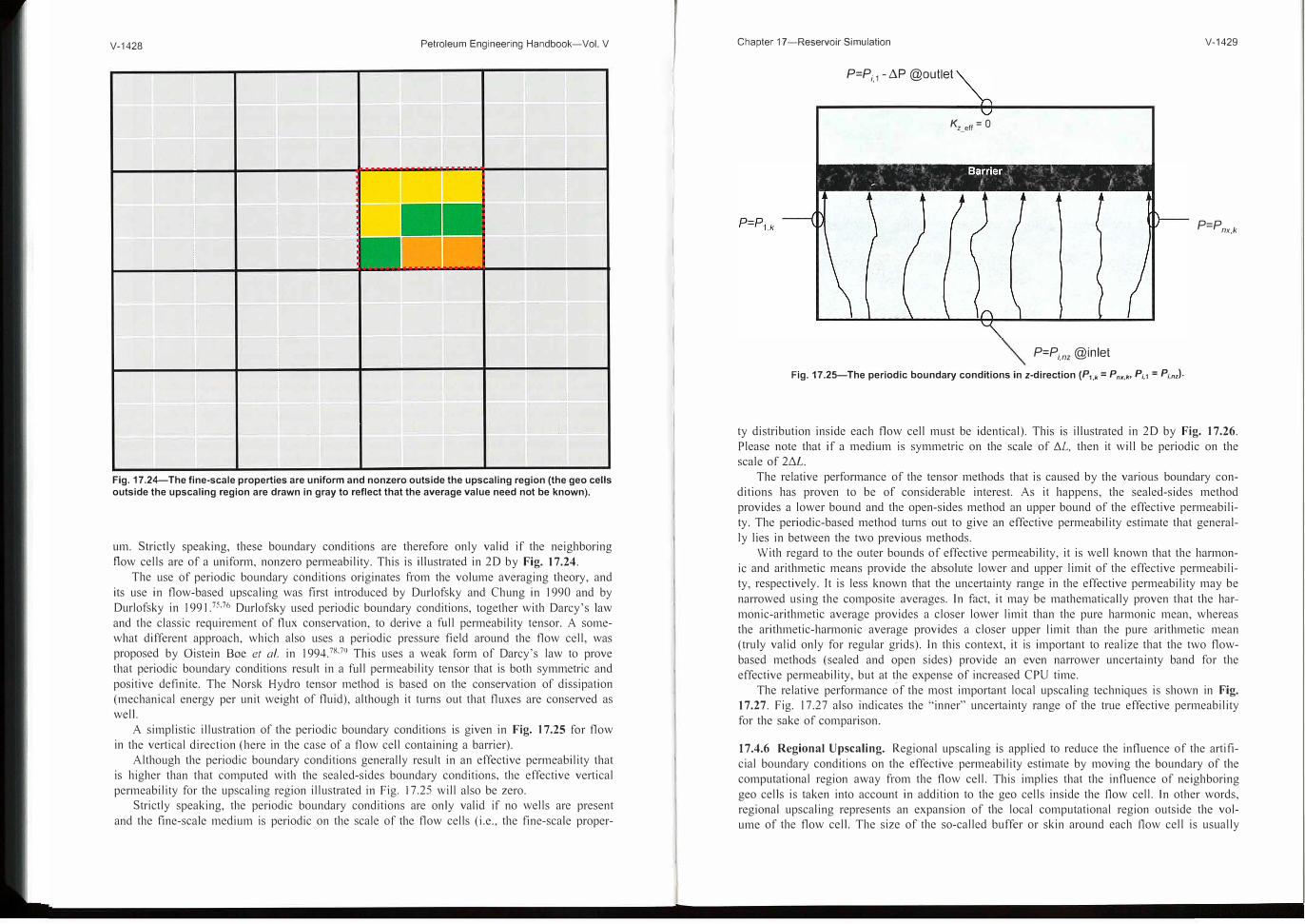
V-1428 Petroleum Engineering Handbook-Vol. V
Fig. 17.24-The fine-scale properties are uniform and nonzero outside the upscaling region (the geo cells outside the upscaling region are drawn in gray to reflect that the average value need not be known).
um. Strictly speaking, these boundary conditions are therefore only valid if the neighboring flow cells are of a uniform, nonzero permeability. This is illustrated in 2D by Fig. 17.24.
The use of periodic boundary conditions originates from the volume averaging theory, and its use in flow-based upscaling was first introduced by Durlofsky and Chung in 1990 and by
Durlofsky in 1991. 75 .76 Durlofsky used periodic boundary conditions, together with Darcy's law and the classic requirement of flux conservation, to derive a full permeability tensor. A somewhat different approach, which also uses a periodic pressure field around the flow cell, was proposed by 0istein Boe et al. in 1994.78
•79 This uses a weak form of Darcy's law to prove
that periodic boundary conditions result in a full permeability tensor that is both symmetric and
positive definite. The Norsk Hydro tensor method is based on the conservation of dissipation (mechanical energy per unit weight of fluid), although it turns out that fluxes are conserved as well.
A simplistic illustration of the periodic boundary conditions is given in Fig. I 7.25 for flow in the vertical direction (here in the case of a flow cell containing a barrier).
Although the periodic boundary conditions generally result in an effective permeability that is higher than that computed with the sealed-sides boundary conditions, the effective vertical permeability for the upscaling region illustrated in Fig. 17.25 will also be zero.
Strictly speaking, the periodic boundary conditions are only valid if no wells are present
and the fine-scale medium is periodic on the scale of the flow cells (i.e., the fine-scale proper-
Chapter 17-Reservoir Simulation V-1429
P=P;, 1 - L'.).p @outlet
K,_err = 0
P=Pnx,k
P=P;,nz @inlet
Fig. 17.25-The periodic boundary conditions in z-direction (P1 ,k = Pn,,k, P;,1 = P;,n,l•
ty distribution inside each flow cell must be identical). This is illustrated in 2D by Fig. I 7.26.
Please note that if a medium is symmetric on the scale of 1"',.l, then it will be periodic on the scale of 2!:,.L.
The relative performance of the tensor methods that is caused by the various boundary conditions has proven to be of considerable interest. As it happens, the sealed-sides method provides a lower bound and the open-sides method an upper bound of the effective permeability. The periodic-based method turns out to give an effective permeability estimate that general
ly lies in between the two previous methods. With regard to the outer bounds of effective permeability, it is well known that the harmon
ic and arithmetic means provide the absolute lower and upper limit of the effective permeability, respectively. It is less known that the uncertainty range in the effective permeability may be
narrowed using the composite averages. In fact, it may be mathematically proven that the harmonic-arithmetic average provides a closer lower limit than the pure harmonic mean, whereas the arithmetic-harmonic average provides a closer upper I imit than the pure arithmetic mean (truly valid only for regular grids). In this context, it is important to realize that the two flowbased methods (sealed and open sides) provide an even narrower uncertainty band for the effective permeability, but at the expense of increased CPU time.
The relative performance of the most important local upscaling techniques is shown in Fig.
17.27. Fig. 17.27 also indicates the "inner" uncertainty range of the true effective permeability for the sake of comparison.
17.4.6 Regional Upscaling. Regional upscaling is applied to reduce the influence of the artificial boundary conditions on the effective permeability estimate by moving the boundary of the computational region away from the flow cell. This implies that the influence of neighboring
geo cells is taken into account in addition to the geo cells inside the flow cell. fn other words, regional upscaling represents an expansion of the local computational region outside the volume of the flow cell. The size of the so-called buffer or skin around each flow cell is usually

V-1432 Petroleum Engineering Handbook-Vol. V
Still, as discussed by Holden and Nielsen,80 the global upscaling approach is not enough to
ensure maximum accuracy in the modeling of the effective permeability. Because the value of
the e ffective permeability is influenced by changes in the pressure field, the flow-cell permeabil
ities should strictly be recomputed by the global method for every timestep taken by the
multiphase flow simulator. In practice, though, it might be good enough to update the effective
permeability field whenever a significant change occurs as a result of altering the well configu
ration or production/injection rates and so on. Hence, the ultimate upscaling scheme for the
absolute permeability might be the one that is coupled with the multiphase flow simulator and
automatically updates the absolute effective permeability field for each timestep. With the cur
rent computer power and the lack of proper integration between the geological model and the
simulation model, this is hardly achievable yet.
17.4.8 Best Practice Guidelines. As may be understood from the previous sections, there ex
ists no single upscaling method for absolute permeability that is superior to all other methods
in all situations, at least not until it has been fully established that the global upscaling scheme
represents the ultimate method of choice. Selecting the proper upscaling method from the many
available choices can be quite a challenge. The choice of sophistication in the upscaling
method generally depends on one or several of the following factors:
• The complexity of the fine-scale permeability distribution (i.e., the geo model).
• The degree of upscaling that needs to be performed (i.e., the coarsening factor).
• The number of permeability realizations that need to be upscaled.
• The time available to the project for performing upscaling.
• The intended use of the flow model.
Because an exact validation of the upscaling process cannot be performed unless a multi
phase flow simulation is carried out on the geo model itself, two alternative upscaling approach
es for identifying the proper homogenization method are presented here.
The Absolute Upscaling Approach. This approach assumes that there exists a way to prop
erly validate the absolute performance of an upscaling method without resorting to an extreme
ly time-consuming (if at all feasible) finite-volume simulation of the geo model. As
documented in Ref. 81, streamline simulation offers a very efficient way of validating the performance of upscaling methods. The validation process is carried out by first running a
streamline simulation on the geo model to compute the reference solution. Then a streamline
simulation is run on the flow model for each of the upscaling methods that are to be evaluated.
The simulated performance of the various upscaling methods is then compared to that of the
geo model. The validation of upscaling methods is best done under single-phase flow condi
tions to avoid introducing other model parameters (e.g., relative permeabilities and associated
rock types) that also need to be upscaled in one way or the other. A higher confidence may
also be obtained for the validation process if the actual well pattern is used in the streamline
simulations.
Using the previously described validation scheme, the modeler may choose to evaluate any
upscaling method until one with a satisfactory performance is found. Still, a more systematic
way of identifying the optimum upscaling method is desirable. With the absolute upscaling
approach that is presented here, the modeler is offered a multistep procedure that is to be termi
nated as soon as a satisfactory upscaling method has been identified. The recommended
procedure involves the following steps:
I. Compute the upper and lower bounds of the effective permeability using the arithmetic
harmonic ( or pure arithmetic) and harmonic-arithmetic ( or pure harmonic) average techniques,
respectively. Being of the analytical type, these methods are very fast and will provide a first
quantification of the upscaling uncertainty. Validate the performance of the two composite meth
ods against that of the geo model using a single-phase streamline simulator with the actual
well pattern.
Chapter 17-Reservoir Simulation V-1433
2. If the performance of any of the two methods in Step is within an acceptable range of
the geo model, then terminate the procedure and choose the appropriate method. If, on the
other hand, the performance of both methods is unsatisfactory because of the complexity of the
geo model, then use the upper (open-sides) and lower (sealed-sides) bound diagonal tensor meth
ods to narrow the uncertainty in the flow-model per formance. Validate the performance of the
two tensor methods against that of the re ference solution.
3. lf the performance of any of the methods in Step 2 is within an acceptable range of the
reference solution, then terminate the procedure and choose the appropriate method. If, on the
other hand, the performance of both methods is unsatis factory, then the following alternatives
may be worth considering:
a. If time allows, refine or coarsen the flow grid (whatever is best) to achieve a better
separation of the length scales. Then repeat the upscaling of the outer bounds (in Step 2) and
redo the validation to check if the performance of either method has improved.
b. Apply a tensor method with periodic or semi-open-boundary conditions [the semi-open
boundary conditions alternative is available in some applications using a multiplier between 0
(sealed) and I ( open) to the side faces of the computational region]. As previously mentioned,
this should result in an intermediate estimate of the effective permeability tensor and therefore
provide a flow model performance that lies somewhere in between the two methods in Step 2.
c. Select the best of the two tensor methods in Step 2 and convert the local method to a
regional method using a buffer region of modest size. Validate its performance. If necessary,
repeat this step using an increasingly larger buffer region until a satisfactory performance of
the flow model is obtained.
d. If for some reason none of the previous alternatives are an option, then one needs to
apply the method that best satisfies the wanted flow behavior of a given cell or cells in a given
region. In other words, a combination of the outer bound techniques within one and the same
model may be a fourth alternative.
As previously mentioned, the method using open-sides boundary conditions is a good esti
mator of sand continuity and quality, whereas the sealed-sides boundary conditions method is
better at detecting the presence and effect of barriers.
Consider a long horizontal oil producer in the Troll West Gas Province that is protected
against coning from the overlying gas cap by a calcite bmTier just above the well. If the verti
cal grid resolution in the Troll full-field model was such that one could apply the open-sides
boundary conditions technique on the cells containing the well, and the sealed-sides boundary
conditions technique on the cells containing the barrier, then this would be the optimum local
upscaling approach.
However, if both a segment of the well trajectory and a segment of the calcite are present
inside the same flow cell, then the open-sides boundary conditions technique will give a good
estimate of the well's PI but result in a much too early gas breakthrough, whereas the sealed
sides boundary conditions method will better capture the effect of the calcite but give a too
low estimate of the well 's Pl. If this is the case, one needs to consider applying one of the
alternatives A or C (alternative B will, in this particular example, give the same result as the
sealed-sides method).
The multistep procedure of the absolute upscaling approach is graphically illustrated in Fig.
17.29.
The Relative Upscaling Approach. This approach acknowledges the fact that an exact vali
dation of the upscaling results cannot be achieved in practice. Therefore, instead of trying to
validate the absolute performance of an upscaling method, the approach diagnoses the relative
performance of outer bound methods using the actual multiphase finite-volume simulator. This
implies that a full black-oil simulation is run on the flow model for each of the upscaling meth
ods that are to be evaluated. The deviation in the simulated performance between outer bound
V-1434 Petroleum Engineering Handbook-Vol. V
k
Compute Kupp and K10w by the
composite procedure
No
Run the single-phase streamline simulator twice
Upscaling performance
OK?
Yes
Recompute Kupp and K10w
by the diagonal tensor procedure
No
Run the single-phase streamline simulator twice
Yes
Recompute Kupp and
K10w by the regional scheme
Compute Kett using semi-open or periodic b.c
Run the single-phase streamline simulator twice
Increase the size of the buffer region
Yes
Establish Kett by combining Kibe and Knbc
Run the single-phase streamline simulator
Ka-h
Kh-a
Refine or coarsen the flow
grid
Fig. 17.29-Flow chart for the absolute upscaling approach.
Chapter 17-Reservoir Simulation V-1435
methods will then reflect the part of the model uncertainty that originates from the upscaling process itself. To ensure a high degree of relevance in the diagnostics, it is important that the test simulations contain a representative description of the actual flow model.
If the project is pressed for time, the simulations may be skipped altogether in favor of a faster, although less robust, way of performing the diagnostics. Instead of analyzing simulation profiles, a normalized difference parameter may be computed on a cell by cell basis using the formula
a =(Kupp-K10)/[(Kurr+K1°')/2] . ......................................... (17.18)
The relative upscaling approach that is presented here utilizes a multistep procedure that applies outer bound methods of increasing accuracy until the best possible upscaling method can be identified. The recommended procedure involves the following steps:
1. Compute the upper and lower bounds of the effective permeability using the arithmeticharmonic ( or pure arithmetic) and harmonic-arithmetic ( or pure harmonic) average techniques, respectively. Being of the analytical type, these methods are very fast and will provide a first quantification of the upscaling uncertainty. Run the finite-volume simulator for each of the two composite methods ( or compute a grid-based difference parameter) and perform the diagnostics.
2. If the performance gap between the two methods in Step I is acceptable (small), thenterminate the procedure and choose either of the two. If the deviation in performance is unsatisfactory because of the complexity of the geo model, then use the upper (open-sides) and lower (sealed-sides) bound diagonal tensor methods to narrow the uncertainty in the flow model performance. Run the finite-volume simulator for each of the two tensor methods ( or compute a grid-based difference parameter) and perform the diagnostics.
3. If this reduces the upscaling uncertainty to within acceptable limits, then either of thetwo diagonal tensor methods may be used to provide the final permeability field for the flow model. If the deviation in the performance is unsatisfactory (large), then the following alternatives may be worth considering:
1. If time allows, refine or coarsen the flow grid (whatever is the best) to achieve a betterseparation of the length scales. Then repeat the upscaling of the outer bounds (in Step 2) and rerun the simulations ( or recompute the difference parameter) to check if the performance gap (upscaling uncertainty) has naiTowed.
2. Apply a tensor method with semi-open or periodic boundary conditions. As previouslymentioned, this should result in an intermediate estimate of the effective permeability tensor and hence provide a flow model performance that lies somewhere in between the two methods in Step 2.
3. Convert the two local tensor methods in Step 2 into regional methods using a bufferregion of modest size. Rerun the finite-volume simulator ( or recompute the difference parameter) and check the performance gap. If necessary, repeat this step using an increasingly larger buffer region until the upscaling uncertainty reaches acceptable limits, at least as far as practically possible.
4. If for some reason none of the previous alternatives are an option, then one needs toapply the method that best satisfies the wanted flow behavior of a given cell or cells in a given region. In other words, a combination of the outer bound techniques within one and the same model may be a fourth alternative.
The multistep procedure of the relative upscaling approach is graphically illustrated in Fig.
17.30.

V-1436 Petroleum Engineering Handbook-Vol. V
k
Compute Kupp and K10w by the
composite procedure
Run the multi-phase finite volume simulator twice
No Upscaling uncertainty
low?
Recompute Kupp and K10w by the
diagonal tensor procedure
Run the multiphase finite volume simulator twice
No
Recompute Kup
p and K10w by the regional scheme
Run the multiphase finite volume simulator twice
Compute Keff using semi-open or periodic b.c
Yes
Yes Use either
Kibe or Knbe
Increase the size of the buffer region
Yes
Use either
Kibe or Knbe
Establish Ken
by combining Kibe and Knbe
Fig. 17.30-Flow chart for the relative upscaling approach.
Use either
Ka-h or Kh-a
Refine or coarsen the flow
grid
Chapter 17-Reservoir Simulation V-1437
17.5 Streamline Simulation-Rod P. Batycky and Marco R. Thiele
17.5.1 Introduction. Streamline-based flow simulation differentiates itself from cell-based simulation techniques such as finite-differences and finite-elements in that phase saturations and
components are transported along a flow-based grid defined by streamlines (or streamtubes)
rather than moved from cell-to-cell. This difference allows streamlines to be extremely efficient
in solving large, heterogeneous models if key assumptions in the formulation are met by the
physical system being simulated (see below). Specifically, large relates to the number of active
grid cells.
Streamlines represent a snapshot of the instantaneous flow field and thereby produce data
such as drainage/irrigation regions associated with producing/injecting wells and flow rate allo
cation between injector/producer pairs that are not easily determined by other simulation
techniques. The computational speed and novel solution data available have made streamlines
an important, complementary approach to traditional simulation approaches to perform sensitiv
ity runs, quantify the impact of upscaling algorithms used to move models from the geomodel
ing scale to the simulation scale, visualize the flow field, perform more reliable full-field
simulations where sector models would normally be used, enable the ranking of predicted field behavior of given multiple production scenarios and input parameters, evaluate the efficiency
of injectors and producers, reduce turnaround time in history matching, and perform other estab
lished reservoir engineering tasks. A comprehensive overview on streamline-based flow simula
tion has recently been presented by Thiele.82
17.5.2 Applicability of Streamline Simulation. The power of streamline simulation lies in its
simplicity. The main objective is to capture how injected reservoir volumes (usually water and/
or gas) displace resident reservoir volumes given well locations, well rates, reservoir geometry,
and geological description. One of the key underlying assumptions in streamline simulation is
that the system be close to incompressibility. This decouples saturations from the underlying
pressure field and allows each streamline to be treated as being independent from the stream
lines next to it.
Many fields under waterflooding or other pressure maintenance schemes are excellent candi
dates for streamline modeling and have been successfully modeled in this way.83•84 Forecast
simulations under the assumption of voidage replacement are another good example where
streamlines can be very effective. Even miscible gas injection schemes have been successfully
modeled.85•86 At high pressures, the displacement of resident oil by gas is primarily an issue of
simulating local sweep efficiency and channeling, something streamlines are designed to model
without incurring numerical difficulties associated with other formulations.87 An early applica
tion to streamdrive projects was presented by Emanuel.88 Crane and Blunt89 used streamlines to
model solute transport. More recently, streamlines have been shown to be very effective in
modeling fractured reservoirs using a dual porosity formulation.90
17.5.3 Historical. Streamlines have been in the petroleum literature as early as Muskat and
Wyckoffs 1934 paper.91 ln 1937, Muskat presented the governing analytical solutions for the
stream function and the potential function for 20 domains using the assumption of incompress
ible flow.92 Since then, streamlines and streamtubes have received repeated attention as a way
to numerically predict the movement of fluids, even after the advent of finite-difference meth
ods in the early I 960s. Important early contributions were made by Fay and Pratts,93 Higgins
and Leighton,94•95 Bommer and Schechter,96 Martin and Wegner,97 Lake et a/., 98 and Emanuel
et al. 99
In the early 1990s, streamlines were revived because advances in geological modeling tech
niques were producing models that were too large for finite differences to simulate in an
acceptable time frame. For streamlines to be applicable to real field cases, important advances

V-1438 Petroleum Engineering Handbook-Vol. V
were made that extended streamlines to 3D using a time-of-flight variable87•
100-
103 allowed for streamlines to be periodically updated87
•104
-105 and included gravity. 106
17.5.4 Mathematics of the Streamline Method. The streamline method and the underlying mathematics for incompressible multiphase flow are briefly outlined here. For a detailed discussion as well as additional references describing streamline methods, see Batycky et al., 87
Batycky, 103 and Blunt et a!. 107
Governing IMPES Equations. The streamline method is an IMPES-type formulation with the pressure field solved for implicitly and the oil/gas/water saturations solved for explicitly along streamlines. The governing equation for pressure, P, for multiphase incompressible flow without capillary or diffusion effects is given by
11 =:
P k k,1 ( __, ) V ·I-· V ·P+p.gD =0, ........................................... (17.19)I/. J
j= I ,- ./
where D is the depth below datum, g is gravitational acceleration constant, k is the permeability tensor, k,i is the relative permeability, Pi is viscosity, and Pi is the phase density of phase j.. -t . . The total velocity, u
1, is derived from the 3D solution to the pressure equation and application
of Darcy's law. The explicit material-balance equation for each incompressible phase j is then given by
as. __, __, ¢ a/ + u , • v .11 + v • a J = 0 . ............................................ ( 11 .20)
Each phase fractional flow, fp is given by
. k,i.fj =
/1-,-1/J--, . . . . . . . . . . . . . . . . . . . . . . . . . . . . . . . . . . . . . . . . . . . . . . . . . . . . . . . . (17.21)
J I k,j; JI.
j= I J
and the phase velocity resulting from gravity effects because of phase density differences 1s given by
11 - p
Gj = k · gfi V DI kJp;-p)IP; . ........................................ (17.22)
i=I
The difference between finite-difference simulation and streamline simulation is the way the explicit material balance equations (Eqs. 17.20 through 17.22) are solved. In finite difference, the material balance equations are solved between gridblocks, whereas in streamline simulation the material balance equations are solved along streamlines. How this is done is explained next.
Solution to the Transport Equation. ln a standard finite-difference method, Eq. 17 .20 is discretized and solved on the underlying grid on which the pressure field is computed. The solution to Eq. 17.20 is governed by the grid CFL condition, which can lead to prohibitively small timestep sizes, particularly for models with high permeability contrasts and/or high local flow velocities. With streamlines, this grid CFL limit is avoided completely by solving Eq. 17.20 along each streamline using a time-of-flight (TOF) coordinate transform. 106
Chapter 17-Reservoir Simulation V-1439
Streamlines are traced from sources to sinks based on the underlying total velocity field. Aseach streamline is traced, compute the TOF along the streamline, which is de fined as
r =/;· 1 ����) 1 dl5 ......................................................... (17.23)
and leads to the de finition
1-:, 1 :;j
= -:,. V = </J ;r . ............................................... (17.24)
Using Eq. 17.19, rewrite Eq. 17.20 as
asi
afi 1 __, _ at+�+¢
V ·G.i-0 . ................................................ (17.25)
Because the gravity term is not aligned along a streamline direction, Eq. 17.25 is split into two paiis ( operator splitting), giving two ID equations. The convective portion of the materialbalance equation along streamlines is given by
asc a f a/+�: = 0, ........................................................... (17.26)
while the portion resulting from phase-density differences solved along gravity lines is given by
asg 1 __, a: +
-;;v ·G.i
= o . ..................................................... (17.27)
Both Eqs. 17 .26 and 17.27 represent ID equations that are solved using standard finite-difference numerical techniques. There are still CFL limits that restrict timestep sizes in these equations, but these are local to each streamline or gravity line, rather then at the 3D grid level.
Timestepping. In field-scale displacements, the streamline paths change with time because of the changing fluid distributions and the changing well conditions. As a result, the total velocity field is periodically updated, and new streamlines are recomputed to reflect the nonlinear nature of the displacement.
To move the 3D saturation distribution forward in time between successive streamline distributions from time T; to T;+i = T; + dT;, the algorithm pictured in Fig. 17.31 is used.
The basic algorithm for streamline-based flow simulation is as follows: (I) Given initial conditions (i.e., pressures and saturations for each active cell in the system) and well conditions, the pressure is solved implicitly for each cell, as is done in conventional finite-difference methods (Eq. 17 .19). (2) With the pressures known, the total velocity for each cell interface can be determined using Darcy's Law. The total velocity is then used to trace streamlines using Pollock's algorithm. 100 (3) ID mass conservation equations are then solved along each streamline, independently of each other (Eq. 17.26). The initial conditions for the streamlines are obtained by a mapping from the underlying 3 D grid onto each streamline. The mass-transport problem is marched forward in time along each streamline for a pre-specified global timestep dT;, and then the solution is mapped back onto the 3D grid. Gravity is included by
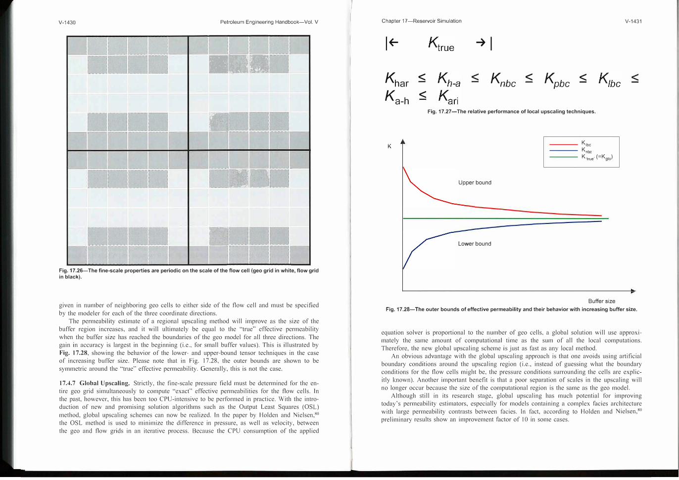
V-1430 Petroleum Engineering Handbook-Vol. V
■■■
■
■■
■
:ig. 17.26-The fine-scale properties are periodic on the scale of the flow cell (geo grid in white, flow grid m black).
given in number of neighboring geo cells to either side of the flow cell and must be specified by the modeler for each of the three coordinate directions.
The permeability estimate of a regional upscaling method will improve as the size of the buffer region increases, and it will ultimately be equal to the "true" effective permeability when the buffer size has reached the boundaries of the geo model for all three directions. The gain in accuracy is largest in the beginning (i.e., for small buffer values). This is illustrated by Fig. 17.28, showing the behavior of the lower- and upper-bound tensor techniques in the case of increasing bu ffer size. Please note that in Fig. 17.28, the outer bounds are shown to be symmetric around the "true" effective permeability. Generally, this is not the case.
17.4.7 Global Upscaling. Strictly, the fine-scale pressure field must be determined for the entire geo grid simultaneously to compute "exact" effective permeabilities for the flow cells. In the past, however, this has been too CPU-intensive to be performed in practice. With the introduction of new and promising solution algorithms such as the Output Least Squares (OSL) method, global upscaling schemes can now be realized. In the paper by Holden and Nielsen,80
the OSL method is used to minimize the difference in pressure, as well as velocity, between the geo and flow grids in an iterative process. Because the CPU consumption of the applied
I ( Chapter 17-Reservoir Simulation
I+-
K < har
Ka-h <
➔I
K < nbc K < pbc
Fig. 17.27-The relative performance of local upscaling techniques.
K
Upper bound
Lower bound
Kibe Kntc K.t,ue" (
=
Kglo)
Buffer size
V-1431
Fig. 17.28-The outer bounds of effective permeability and their behavior with increasing buffer size.
equation solver is proportional to the number of geo cells, a global solution will use approximately the same amount of computational time as the sum of all the local computations. Therefore, the new global upscaling scheme is just as fast as any local method.
An obvious advantage with the global upscaling approach is that one avoids using artificial boundary conditions around the upscaling region (i.e., instead of guessing what the boundary
�onditions for the flow cells might be, the pressure conditions surrounding the cells are explicitly known). Another important benefit is that a poor separation of scales in the upscaling will no longer occur because the size of the computational region is the same as the geo model.
Although still in its research stage, global upscaling has much potential for improving today's permeability estimators, especially for models containing a complex facies architecture with large permeability contrasts between facies. In fact, according to Holden and Nielsen 80
preliminary results show an improvement factor of IO in some cases. '
V-1440
Well conditions at
time T;
OJC 0 ro gi 0. C Ql
=
u5 EQl Cll> �t5 en Ql oiE: c:: 0 ()
OJC 0 ro gi 0. C Ql
=
u5 EQl Cll> �nmQl -> 0, C C::0
Petroleum Engineering Handbook-Vol. V
I
Initial condition
Pressure solve (Eq. A-1)
Trace streamline
1 D solver (Eq. A-8)
Map new streamline saturations to grid
I�----� -- - -� L _____ _
I
I
I
I
I I
I
I
I I
Trace gravity line
1 D solver (Eq. A-9)
I,------�------, 1 Map new gravityline I saturations to grid I�----�--- -� L _____ _
End simulation
Update time to
°T;+1 = T;+dT;
Fig. 17.31-Flow chart showing the basic algorithm for streamline-based flow simulation.
considering a vertical segregation step along gravity lines after movement along all streamlines
(Eq. 17.27). While simple in its approach, important details must be considered. In particular:
1. The algorithm is similar to an IMPES approach, in that the pressure is solved implicitly
for a new time level 11+ l assuming saturations at level n. The saturations at time n are given
by mapping back solutions from each streamline onto the 3D grid at the previous timestep.
Because of the implicit nature of the pressure solution, there is no limitation on the timestep to
reach 11+ 1. However, for compressible systems numerical convergence problems might limit the
actual size of the timestep. This is no different than in FD simulation.
2. The tracing of the streamlines using Pollock's algorithm assumes Cartesian cells.
Nonorthogonal corner-point cells require an isoparametric transformation for tracing
streamlines. 108
3. For incompressible systems, streamline will start at injection wells and end at production
wells. For compressible systems, streamline can start/end anywhere in the system, because any
Chapter 17-Reservoir Simulation V-1441
gridblock in the system might act as a source (volume expansion) or a sink (volume contrac
tion). Multiphase gravity e ffects can give rise to circulation cells for both incompressible and
compressible systems.
4. Initial launching of streamlines from wells can be proportional to the total flux at the
wells, though this will in general leave many cells in the system without a streamline passing
through them. For missed cells, tracing begins at the center of the missed cell and then traced
backward until a source is encountered. lf a cell does not have a streamline pass through it,
then it is not possible to assign an updated saturation back to that cell.
5. In practice, it is not possible to have all streamlines carry the same flux and ensure at
least one streamline per cell. Thus, streamlines do not carry the same flux. Furthermore, for
incompressible problems the flux along each streamline is a constant, while for compressible
systems it is not.
6. The tracing of streamlines using the TOF variable produces a highly irregular ID grid
along each streamline. To numerically solve the ID problem efficiently, the ID grid must be
regularized, solved using an implicit approach, or regridded in some way to allow for a more
efficient solution.
7. The tracing of the streamlines relies on an accurate solution of the velocity field. Exces
sive distortions of the grid (nonorthogonal) or a pressure solution that has not been solved to a
small enough tolerance can cause problems in tracing streamline paths.
17.5.5 The Computational Efficiency of Streamlines. One advantage of streamline simulation
over more traditional approaches is its inherent efficiency, both in terms of memory and com
putational speed. Specifically, streamline-based simulation can exhibit a near-linear scaling in
run times as a function of active cells in the model. Memory efficiency is a result of two key
aspects of the formula: streamline-based simulation is an JMPES-type method and therefore
involves only the implicit solution of pressure, and tracing of streamlines and solution of the
relevant transport problem along each streamline is done sequentially. Only one streamline
needs to be kept in memory at any given time.
Computational speed, on the other hand, is achieved because the transport problem is decou
pled from the 3D grid and instead solved along each streamline. Because transpo1i along
streamlines is ID, they can be solved efficiently. Because the number of streamlines increases
linearly with the number of active cells, and streamlines only need to be updated infrequently,
the computational time exhibits a near-linear scaling with increasing number of gridblocks
The number of global timesteps is related to how often the flow field (streamlines) requires
updating. Specifically, changing flow paths are a function of heterogeneity, mobility changes,
gravity, and changing well conditions. For many practical problems, it is the changing well
rates that introduced the greatest impact on a changing flow field and is therefore the limiting
factor in deciding on global timestep sizes. Grouping well events into semiyearly or yearly
intervals and assuming that the streamlines remain unchanged over each period is reasonable.
This is why field simulations with 30- to 40-year histories are successfully and routinely simu
lated with I -year timesteps. 84
A good example to demonstrate the efficiency of SL simulation is Model 2 of the I 0th
SPE comparative solution project. 12 The total run time, T, of any streamline simulation is ap
proximately proportional to
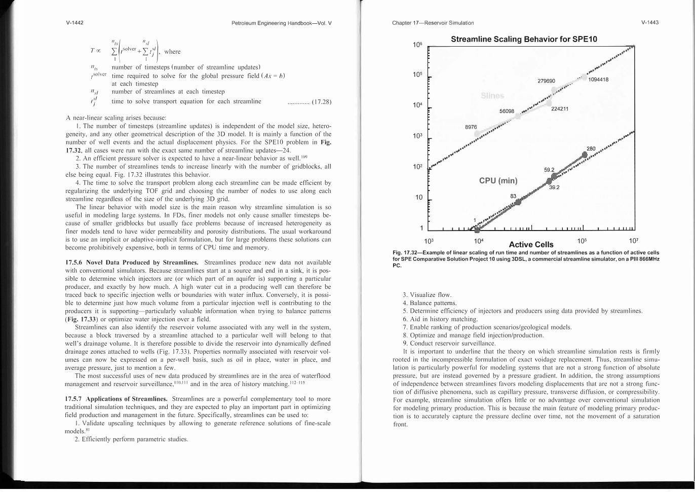
V-1442
Trx
11,s 1solver
n,'i
r''
J
Petroleum Engineering Handbook-Vol. V
111 ( 11 / )
�1
· !solver +� t)' ' where
number of timesteps (number of streamline updates) time required to solve for the global pressure field (Ax = b) at each timestep number of streamlines at each timestep time to solve transport equation for each streamline ............. (17.28)
A near-linear scaling arises because: I. The number of timesteps (streamline updates) is independent of the model size, hetero
geneity, and any other geometrical description of the 3 D model. It is mainly a function of the number of well events and the actual displacement physics. For the SPE IO problem in Fig.
17.32, all cases were run with the exact same number of streamline updates-24. 2. An efficient pressure solver is expected to have a near-linear behavior as well.109
3. The number of streamlines tends to increase linearly with the number of gridblocks, allelse being equal. Fig. 17.32 illustrates this behavior.
4. The time to solve the transport problem along each streamline can be made efficient byregularizing the underlying TOF grid and choosing the number of nodes to use along each streamline regardless of the size of the underlying 3D grid.
The linear behavior with model size is the main reason why streamline simulation is so useful in modeling large systems. In FDs, finer models not only cause smaller timesteps because of smaller gridblocks but usually face problems because of increased heterogeneity as finer models tend to have wider permeability and porosity distributions. The usual workaround is to use an implicit or adaptive-implicit formulation, but for large problems these solutions can become prohibitively expensive, both in terms of CPU time and memory.
17.5.6 Novel Data Produced by Streamlines. Streamlines produce new data not available with conventional simulators. Because streamlines start at a source and end in a sink, it is possible to determine which injectors are (or which part of an aquifer is) supporting a particular producer, and exactly by how much. A high water cut in a producing well can therefore be traced back to specific injection wells or boundaries with water influx. Conversely, it is possible to determine just how much volume from a particular injection well is contributing to the producers it is supporting-particularly valuable information when trying to balance patterns (Fig. 17.33) or optimize water injection over a field.
Streamlines can also identify the reservoir volume associated with any well in the system, because a block traversed by a streamline attached to a particular well will belong to that well's drainage volume. It is therefore possible to divide the reservoir into dynamically defined drainage zones attached to wells (Fig. 17.33). Properties normally associated with reservoir volumes can now be expressed on a per-well basis, such as oil in place, water in place, and average pressure, just to mention a few.
The most successful uses of new data produced by streamlines are in the area of waterflood management and reservoir surveillance, 1 10·111 and in the area of history matching. 1 12
-115
I 7.5.7 Applications of Streamlines. Streamlines are a powerful complementary tool to more traditional simulation techniques, and they are expected to play an important part in optimizing field production and management in the future. Specifically, streamlines can be used to:
I. Validate upscaling techniques by allowing to generate re ference solutions of fine-scalemodels.81
2. Efficiently perform parametric studies.
Chapter 17-Reservoir Simulation
1Q6
1Q5
104
103
102 ,.,,. ,.,,.,
10
103
Streamline Scaling Behavior for SPE10
56098
�-,,-·· 8976 +··+
+·· +··
+·· +""
+··
.;•" .,,4•
""'
CPU (min)
279690
.,,4•
+' •.. .....
+· ,.
1T•••
""' .....
2242.1j
104
Active Cells 105
........
+" +··
+·· .;•"
,""'
1094418
107
V-1443
Fig. 17.32-Example of linear scaling of run time and number of streamlines as a function of active cells
for SPE Comparative Solution Project 10 using 3DSL, a commercial streamline simulator, on a Pill 866MHz
PC.
3. Visualize flow.4. Balance patterns.5. Determine efficiency of injectors and producers using data provided by streamlines.6. Aid in history matching.7. Enable ranking of production scenarios/geological models.8. Optimize and manage field injection/production.9. Conduct reservoir surveillance.It is important to underline that the theory on which streamline simulation rests is firmly
rooted in the incompressible formulation of exact voidage replacement. Thus, streamline simulation is particularly powerful for modeling systems that are not a strong function of absolute pressure, but are instead governed by a pressure gradient. In addition, the strong assumptions of independence between streamlines favors modeling displacements that are not a strong function of diffusive phenomena, such as capillary pressure, transverse diffusion, or compressibility. For example, streamline simulation offers little or no advantage over conventional simulation for modeling primary production. This is because the main feature of modeling primary production is to accurately capture the pressure decline over time, not the movement of a saturation front.

V-1446 Petroleum Engineering Handbook-Vol. V
17.6.2 Modeling of Reservoir Compaction and/or Dilation. Modeling reservoir deformation
is of considerable importance in soft and/or thick reservoirs where the results of compaction
may provide an important production mechanism, cause well failures, and/or cause ground sub
sidence or heave with environmental consequences. Review of the compaction mechanics and
its consequences for field development is found in Ref. 121. Initial approach to modeling com
paction was based on modifications of reservoir models.122-
125 The common feature of such
reservoir compaction models is that the compaction is treated as a ID problem (uniaxial strain)
by assuming that (a) only vertical deformations take place, and (b) each vertical column of
blocks deforms independently. In such models, the porosity changes are calculated by modify
ing the conventional compressibility cR as a function of pressure only, in the form of
"compaction tables." The tables are based on results of uniaxial strain laboratory experiments,
and the stress problem is not solved. The compaction of the reservoir is then obtained analyti
cally assuming uniaxial deformation. The relation between reservoir compaction and surface
subsidence can be then obtained by an independent solution of a stress problem using the com
puted compaction as a boundary condition. Dilation (increase of porosity) is an important
geomechanical mechanism occurring during steam injection into unconsolidated sands. This pro
cess has been also modeled by the "compaction-dilation" tables.126 In chalk reservoirs, in
creased water saturation in waterflooding causes weakening of the rock and therefore Sw is an
additional variable in Eq. 17 .32. 127
The major drawback of the use of compaction tables is that the dependence on stress indi
cated in Eq. 17.32 must be either ignored, or the change of stress must be estimated in terms
of change in pressure. A more accurate modeling approach is to couple in some fashion the
reservoir simulator with stress-strain (geomechanics) solution. Such models typically combine
the solution of the multiphase flow in the reservoir and elastoplastic solution of the defonna
tions in a much larger domain including the reservoir, sideburden, underburden, and overbur
den. The majority of coupled models use the iterative coupling 128; the different variations and
their shortcomings are discussed next.
Coupled models have much larger computing requirements compared with a reservoir mod
el of the same reservoir, primarily for two reasons: first, the larger number of unknowns per
gridblock, and second, the stress-solution grid must be usually much larger laterally than the
reservoir grid to eliminate the effect of boundary conditions as well as extend up to surface to
provide subsidence solution. Combination of these factors leads to computing times typically of
one order of magnitude larger compared with conventional simulation, and even more if elasto
plastic solution is required for the stresses.
17.6.3 Modeling of Stress-Dependent Flow Properties. The primary flow-dependent property
is permeability, and the problems to model its dependency in Eq. 17.33 are similar to modeling
the pore-volume coupling (Eq. 17.32). However, the problem is somewhat easier because stress
dependent permeability (or transmissibility) does not affect mass-balance formulation.
Again, the traditional approach is to use tables of le vs. pressure in an uncoupled model.
However, the problem remains one of replacing the dependency on effective stress by one on
pressure only. Even in a single-phase, single-porosity gas-flow case, different assumptions
about the stress change during depletion can lead to large errors in well decline.129 Different
strategies for converting the stress-dependent data to pressure tables are based on local constrain
ment assumptions. 130
In coupled models, the permeability dependency can be usually computed explicitly on a
timestep basis, and "loose" coupling can be used. In fact, a "coupled" model that deals only
with flow properties coupling and ignores the pore-volume coupling can be run successfully
even if the stress solution is done in larger intervals of time compared to the reservoir. Such
models have been used extensively to study permeability changes in watertloods, particularly
Chapter 17-Reservoir Simulation V-1447
in fractured or jointed media. 131•132 Here, the advantage of coupled modeling is in its capability
to predict the permeability changes from the geomechanics of reopening of fractures or failure
(dilation) of joints.133 The development of anisotropy is dictated by the orientation of fractures
or faults, and requires a "full tensor" treatment of transmissibilities in the flow model. ln the
stress strain model, different methods of pseudoizing the fracture/joint networks into a continu
um are used, which include predicting permeability as a function of effective stress and/or
strain. While the need for the tensor transmissibilities in such models has been recognized, 134
in injection processes dual-porosity media can be created. Therefore, reservoir description may
be changing in time because of geomechanics; this aspect has been ignored in coupled models
to date.
The same principles can be also applied to model hydraulically induced fractures being rep
resented by dynamically changing transmissibility multipliers in the potential fracture plane. 135
The effective stress dependency (as opposed to pressure in an uncoupled model) allows captur
ing the changes of the fracture propagation pressure with time, which can be large, in particu
lar in steam injection. Another application is the prediction of production/injection-induced
slippage on faults, which can induce communication between reservoir fault blocks and/or seis
micity.
17.6.4 Types of Coupled Models. Coupled models can be either fully coupled (i.e., all un
knowns solved simultaneously) or modular (reservoir simulator and stress code). In the latter
case, different coupling strategies can be used, with consequences for running speed and accu
racy. The majority of coupled models use a conventional finite-difference reservoir simulator
coupled with a finite-element (FEM) stress simulator. However, attempts have been made to
develop fully coupled FEM codes,136 and a fully coupled geomechanics was implemented in a
commercial model using a finite-difference stress solution.137 Considering the proliferation and
sophistication of the geomechanics codes available outside the petroleum engineering, the mod
ular approach offers the best solution.119•127 Generally, the reservoir simulator is the "host" or
"master." Commercial stress simulators are, in principle, easy to couple to it (in particular if
only permeability coupling is considered).
Because of the extreme complexity and large computing requirements of coupled models,
different simplifications have been developed. The main types of models (in the order of in
creasing rigorousness, but also computing time) are as follows:
One-Way Coupling. Pressure and temperature changes are passed from the reservoir code
to the geomechanics module, but no information is passed back on timestep basis. The geome
chanics does not improve the flow solution, but the model can be useful for predictions of
well bore stability for infill drilling, fracturing pressures, and so on. Manual adjustment of "com
paction tables" is possible manually through restarts. Such manually coupled solutions 138 of the
stress problem (at intervals of time) or one-way coupling139 were often used in early coupled
modeling. The method can be satisfactory when the reservoir fluid system is highly compress
ible (i.e., in gas reservoirs), but can lead to errors when the porosity is strongly coupled to flow.
Loose Coupling. Reservoir and geomechanics modules are run sequentially on a timestep
basis, passing converged solutions of flow and stress variables to each other. Pore volumes and
permeabilities in the flow model are computed as a function of p, T, and aavg with stress vari
ables lagged a timestep. However, the relationships are "distilled" into tables similar to the
"compaction tables," but now a function of effective stress. The advantages are functional simi
larity to the uncoupled reservoirs with "compaction tables," no need for iteration during
timestep, and the possibility of updating the stress solution less frequently than the reservoir
solution. However, complex constitutive models of the solid (e.g., plasticity) may be difficult
to represent.
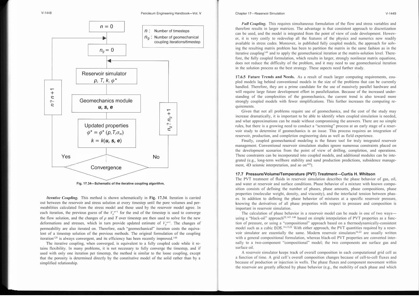
V-1448
..--+
C:
C--•
C:
Yes
n 0
Reservoir simulator
p, T, k, ¢*
Geomechanics module u,s, e
Updated properties
¢* = ¢* (p, T,am)
k = k(u, s, e)
Petroleum Engineering Handbook-Vol. V
n : Number of timesteps
n9 : Number of geomechanical
coupling iterations/timestep
No
..--+
C:
0,
C:
Fig. 17.34-Schematic of the iterative coupling algorithm.
Iterative Coupling. This method is shown schematically in Fig. 17.34. Iteration is ca1Tied out between the reservoir and stress solution at every timestep until the pore volumes and permeabilities calculated from the stress model and those used by the reservoir model agree. In each iteration, the previous guess of the V,,11• 1 for the end of the timestep is used to converge
the flow solution, and the changes of p and T over timestep are then used to solve for the new deformations and stresses, which in turn provide updated estimate of V,,11• 1• The changes of
permeability are also iterated on. Therefore, each "geomechanical" iteration costs the equivalent of a timestep solution of the previous methods. The original formulation of the coupling iteration 128 is always convergent, and its efficiency has been recently improved. 140
The iterative coupling, when converged, is equivalent to a fully coupled code while it retains flexibility. In many problems, it is not necessary to fully converge the timestep, and if used with only one iteration per timestep, the method is similar to the loose coupling, except that the porosity is determined directly by the constitutive model of the solid rather than by a simplified relationship.
Chapter 17-Reservoir Simulation V-1449
Full Coupling. This requires simultaneous formulation of the flow and stress variables and therefore results in larger matrices. The advantage is that consistent approach to discretization can be used, and the model is integrated from the point of view of code development. However, it is very costly to redevelop all the features of the physics and numerics now readily available in stress codes. Moreover, in published fully coupled models, the approach for solving the resulting matrix problem has been to partition the matrix in the same fashion as in the iterative coupling 141 and to apply the geomechanical iteration at the matrix-solution level. Therefore, the fully coupled fonnulation, which results in larger, strongly nonlinear matrix equations, does not reduce the difficulty of the problem, and it may need to use geomechanical iteration in the solution process as the best strategy. These aspects need further study.
17.6.5 Future Trends and Needs. As a result of much larger computing requirements, coupled models lag behind conventional models in the size of the problems that can be cu!Tently handled. Therefore, they are a prime candidate for the use of massively parallel hardware and will require large future development effort in parallelization. Because of the increased understanding of the complexities of the geomechanics, the cu1Tent trend is also toward more strongly coupled models with fewer simplifications. This further increases the computing requirements.
Given that not all problems require use of geomechanics, and the cost of the study may increase dramatically, it is important to be able to identify when coupled simulation is needed, and what approximations can be made without compromising the answers. There are no simple rules, but there is a growing need to conduct a "screening" process at an early stage of a reservoir study to determine if geomechanics is an issue. This process requires an integration of reservoir, production, and completion engineering data as well as field experience.
Finally, coupled geomechanical modeling is the future tool for truly integrated reservoir management. Conventional reservoir simulation studies ignore numerous constraints placed on the development scenarios from the point of view of drilling, completion, and operations. These constraints can be incorporated into coupled models, and additional modules can be integrated ( e.g., long-term well bore stability and sand production predictions, subsidence management, 4D seismic interpretation, and so on 142).
17.7 PressureNolume/Temperature (PVT) Treatment-Curtis H. Whitson
The PVT treatment of fluids in reservoir simulation describes the phase behavior of gas, oil, and water at reservoir and surface conditions. Phase behavior of a mixture with known composition consists of defining the number of phases, phase amounts, phase compositions, phase properties (molecular weight, density, and viscosity), and the interfacial tension between phases. In addition to defining the phase behavior of mixtures at a specific reservoir pressure, knowing the derivatives of all phase properties with respect to pressure and composition is important in reservoir simulation.
The calculation of phase behavior in a reservoir model can be made in one of two waysusing a "black-oil" approach22• 143-146 based on simple interpolation of PVT properties as a function of pressure, or using a "compositional" approach based on a thennodynamically-consistent model such as a cubic EOS. 14• 15 •22 With either approach, the PVT quantities required by a reservoir simulator are essentially the same. Modern reservoir simulators14•22 are usually writtenwith a general compositional formulation, whereas black-oil PVT properties are converted internally to a two-component "compositional" model; the two components are surface gas and surface oil.
A reservoir simulator keeps track of overall composition in each computational grid cell as a function of time. A grid cell's overall composition changes because of cell-to-cell fluxes and because of production or injection in wells. The phase fluxes and component movement within the reservoir are greatly affected by phase behavior ( e.g., the mobility of each phase and which
V-1450 Petroleum Engineering Handbook-Vol. V
components are carried in each phase). The surface products from wells are dependent on the phase behavior of produced wellstreams, but at conditions far removed from reservoir pressure and temperature.
In most reservoir simulators, the water phase and water component are treated in a simplified manner-namely, that the water component does not partition into the hydrocarbon phases, and the hydrocarbon components do not partition into the water phase; the term "hydrocarbon" also includes N2, CO2, and H2S. Because of relatively high CO2 solubility in water, and the potential importance of CO2 "accounting" in CO2 floods, some compositional models allow CO2 paiiitioning in the water phase.147
Conceph1ally and computationally, it is feasible to allow complete partitioning of all components in all phases in reservoir simulation. The partitioning related to the water phase and the water component could be treated with simple pressure-dependent tables, or even with an EOS model. The water-related K-values have simple composition dependence that would make EOSbased fugacity updates almost trivial. The main problem would be treating the impact of changing salinity on water-related K-values. From a practical point of view, however, modeling water-related component partitioning will have a marginal impact on reservoir performance. Hereafter, only phase behavior of nonaqueous phases will be discussed.
17.7.1 Number of Phases and Phase Type. The staiiing point for PVT calculations in a model grid cell is to detennine if the overall composition is single-phase or two-phase at the current pressure estimate. If a cell is single-phase, the phase "type" (gas or oil) may also be needed to select the proper relative permeability and capillary pressure curves. For a black-oil PVT model (i.e., any model with simple pressure-dependent K-values), dete1111ining the number of phases and phase identification is trivial.
For EOS models, two methods can be used for establishing how many phases exist: the Michelsen 148 phase stability test or a sah1ration pressure calculation. 148 The stability test is relatively "slow" because good K-value estimates are not used to initiate the calculation, whereas a saturation pressure can be quite fast because good K-value estimates are often available. A stability test is more reliable in the sense of giving a conclusive result, whereas a near-critical saturation pressure test may not be found149 or converge correctly to a nontrivial solution. Another advantage of using saturation pressure is that it gives a consistent method to define phase type for single-phase cells, something that is not provided by the stability test. The choice of which method to use depends on the tradeoff between speed and reliability. Both methods, if detecting two phases, give excellent starting K-values to initiate the two-phase flash calculation.
17.7.2 Two-Phase Flash. Having established that two phases exist in a cell, one must perform a flash calculation. The flash calculation uses the overall moles n and molar composition z; to determine the molar amounts of each phase (n
g and n
0), and the phase compositions (y; and x;).
For simple pressure-dependent K-value models, the Rachford-Rice150·151 (RR) procedure is usedto find molar amounts and compositions,
N N z;(K; - 1)L (yi - x) = L 1 + a. (K _ l ) = 0, ......................................... (17.34)i= I i= I g I
solving for a.g
= ng
I (ng
+ n0
), with X; = z; I [ 1 + a.g(K; - 1 )] and Y; = K; x;.152
For an EOS model, using the RR solution can be used, but an additional constraint must be satisfied; the fugacity of each component must be the same in each phase, 153 /g; = J
0;. Using an
initial set of K; estimates, the RR equation is solved. Resulting compositions y and x are then used to calculate fugacities }�; and J;,;• If the constraint /g; = J;,; is not satisfied for all compo-
Chapter 17-Reservoir Simulation V-1451
nents, a new set of K-values is estimated usmg some form of a successive substih1tion (SS) update K;ncw = Kiold(J;,; I}�;).
For reservoir simulation, a Newton solution of the flash equation should be much faster than SS methods. Including the equal-fugacity constraint within the set of nonlinear equations used to solve for model pressures "automatically" provides the first Newton update of the flash equation.153 Usually only one additional Newton iteration of the flash equation is needed to converge the fugacity constraints to required tolerance.
In summary, K-values alone determine the phase amounts and phase compositions (from the Rachford-Rice equation). The EOS model guarantees rigorous thennodynamic consistency through the equal-fugacity constraint, ensuring that K-values properly account for pressure and composition dependence of the phase split and component partitioning.
Having completed the flash calculation in a cell, the following information is known: phase moles, phase masses, phase densities, phase volumes (saturations), and phase compositions. The viscosity and gas/oil IFT can be calculated using compositional correlations, 152 or interpolated from pressure-dependent tables for a black-oil model. The impact of PVT properties on reservoir performance will consider individual PVT properties and their impact on individual ten11S in the flow equations.
17.7.3 Density. Phase molar amounts, ng
and nm are converted to phase volumes using phase molecular weights and densities: v
g = niff
g I P
g and V
o = nOMO I Pm where s
g = v
g I vblock and
S0
= V0
I Vblock· Saturations determine relative permeabilities, which can have a dramatic impact on phase fluxes. Typically, le,. - S", where n - 2 to 4. For n = 3, a 5% error in density results in a 15% error in le,..
For reservoirs with sufficiently high vertical permeability, gravity will often play an important role in recovery. Gravity segregation is caused by vertical fluxes driven by the potential tenns V P
g = d(p
g + p
ggz + P,gu) I dz, V p
O = d(p
O + p,,gz) I dz, and V Pw = d(p"' + p
11gz +
Pell'(,) I dz. Errors in densities have a direct impact on gravity segregation. It is actually the density difference between flowing phases that determines the magnitude of gravity segregation (i.e., !::,.p
11,0 = Pw - Pm !::,.pg0
= p0 -
Pg, and !::,.p
wg = Pw - Pg). Likewise, the condition for equilibri
um initialization V Pg
= V p0
= V p11
, = 0 results in saturation-depth distributions, which must honor input !::,.p
g� = P,
go(S
g) and !::,.p,\(,g = PmoCS11 ,) relationships.
A +5% error in oil density (e.g., 630 instead of 600 kg/m3) and a -5% in gas density (e.g., 380 instead of 400 kg/m3) results in gravity segregation potential (!::,.P
go = p0
- Pg) in error by
25% (250 instead of 200 kg/m3). Similarly, in the initialization of a water/oil system, the inadvertent use of p
11• = 62.5 lbm/ft3 instead of the correct value of 70.0 lbm/ft3 for a high-salinity
brine could easily cause a 25% error in initial oil in place for a low-penneability (large capillary transition zone), low-API oil.
In black-oil models, it is particularly easy to model densities incorrectly because of the inadvertent use of "arbitrary" surface densities. The reservoir phase densities are not input directly in a black-oil model. Instead, they are calculated using the formation volume factors (FVF) Bm B
g, and B11,, solution gas/oil and oil/gas ratios Rs and r,, and surface densities P
g"' Pos, and Pw,·, based on the relations Pg
= (pg,· + Pus rs) I B
g, p
0 = (p
0_, + R_, P
g.J I Bm and Pw = Pll's I
B11
,. Because reservoir densities are not usually tabulated as output by reservoir simulators, the user may not know how "wrong" the densities might be.
A well-hmed EOS using volume shift factors154 should always predict reservoir and surface densities within 2 to 4%, and often within I to 2%. The author's experience has found it generally unnecessary to use different volume shift factors for reservoir and surface calculations unless all densities are needed with accuracies of l to 2%. The use of either Peng-Robinson 155 or Soave-Redlich-Kwong156 EOS with volume-shift factors provides densities as good or betterthan the more-complicated ZJRK157 EOS model; in this author's opinion, the ZJRK no longer

V-1452 Petroleum Engineering Handbook-Vol. V
has a role in reservoir simulation, as supported by decreasing industrial use (almost to nonexistent) during the past 5 years.
17.7.4 Component Partitioning. The part1t1oning of components in gas and oil phases, as dictated by K-values, is important for properly describing vaporization and condensation. Vaporization is the process of "stock-tank oil" (STO) components (C6,) moving from the oil phase to
the gas phase, while condensation is the process of intennediate (C3-C 10+) components moving
from the gas phase to the oil phase. Retrograde condensation is particularly important in the depletion of gas condensate reservoirs, where in-situ retrograde condensation results in decreasing surface liquid yields.22, 152, 158
For most gas-injection projects, vaporization will play an important role. Proper modeling of vaporization usually requires a compositional model that uses a detailed description of the heavier (C7+) components, typically three to five fractions.22• 159• 160 The lightest fractions (C7 toC12) will typically vaporize 80 to I 00%, while intennediate heavies (C 13 to C20) may vaporize in varying amounts from 30 to 90%, and the heaviest components C20+ may vaporize from O to 50%. The degree of vaporization depends primarily on the local pressure and composition of displacing gas. Cook et al. 144 suggested a modification of the black-oil model that allows saturated properties to change as a function of how much injection gas has contacted a given cell, thereby allowing reasonable description of a vaporization-dominated process. Tang and Zick 16 1
propose a limited three-component compositional model that allows accurate description of developed miscibility for use in models in which grid-related dispersion may result in underpredicted conditions of miscibility using an EOS-based simulator.
In some gas-injection processes, the injection gas may be enriched (I) during injection by adding NGLs (C3 to C5 components) and/or (2) within the reservoir by multiple contacts with reservoir oil, which gradually enriches the injection gas with intermediate components C3 through C10. For either type of enrichment, the vaporization process can become extremely efficient and result in a near-miscible or miscible displacement with near-I 00% recovery of the oil. When such a displacement results, it is often associated with the development of a complex process whereby the near-miscible front consists of upstream vaporization and downstream condensation-the "condensing/vaporizing" gas drive mechanism first described by Zick. 162
For an EOS model to properly describe complex phase behavior related to vaporization, condensation, and near-miscible mechanisms, special PVT experimental data should be measured and used to tune the EOS. For immiscible processes with significant vaporization, a singlecell multicontact PVT test is useful, quantifying the degree of vaporization in terms of oil volumetric stripping and gas compositional changes. For near-miscible or miscible processes, a swelling-type test which has the following features is strongly recommended: (I) five to seven mixtures of reservoir oil and injection gas are used, with two to three mixtures being bubblepoints and two to three mixtures being dewpoints; (2) a constant composition expansion is conducted on each mixture, where saturation pressure and the oil relative volumes are measured and reported; and (3) a single equilibrium "flash" somewhat near the critical point is used for obtaining a set of equilibrium gas and oil compositions (K-values).
Proper EOS tuning of the complex phase behavior measured in such an experiment is difficult, and requires the ability to match near-critical volumetric and compositional changes. Such predictions are almost never available a priori with an EOS model that has been tuned only to simple depletion data. Small but important modifications of the heavy-end properties and binary interaction parameters are usually required to obtain a satisfactory match of near-critical PVT data provided by this special "swelling" test. A tuned EOS model that is able to match all PVT data, including near-critical phase behavior, has a good chance of properly predicting true multicontact near-miscible/miscible behavior. 152,162
Chapter 17-Reservoir Simulation V-1453
17.7.5 Viscosity. Gas viscosities are typically estimated by correlation 152 within 5 to I 0%, and they are almost never measured experimentally. Such accuracy is adequate for most applications, and gas viscosities seldom vary beyond the range of 0.02 to 0.03 cp. For gas-injection processes at high pressure or near-miscible displacements, gas viscosities can range from 0.03 to 0. 1 cp. Gas-viscosity correlations are not usually accurate for this higher range of viscosity, and errors up to 20 to 30% may be expected; compositional viscosity correlations also have the same level of accuracy.
Oil viscosities are notoriously inaccurate based on correlations, 152 at best being within IO to 30%, but often in error by 50% or more. Oil viscosities should always be measured and used to tune a viscosity model. A minimum requirement would be measurement of stock-tank oil viscosities, and nonnally live-oil viscosities are available from a differential liberation test.
For gas condensates, oil viscosities are almost never measured. This may be a serious problem if condensate blockage has a significant impact on well deliverability. 163 Condensate viscosities are difficult to measure because retrograde condensate volumes can be very small. The use of a separator condensate sample is recommended. Bring it to reservoir conditions (T
and P) for density and viscosity measurements, then tune the viscosity model to these data. This approach is feasible for any gas condensate; it is not expensive, and it is better than relying on untuned compositional viscosity correlations.
Our experience has been that the compositional viscosity correlation by Lorenz, Bray, and Clark 164 (LBC) is not predictive, and it is highly dependent on accurate density predictions. Tuning the heavy-component critical volumes and, sometimes, careful modification of the higherorder constants in the LBC equation, provide the required accuracy for gas and oil viscosities in most reservoir processes. Unfortunately, modification of the LBC correlation to match a limited number of viscosities (in a narrow range of pressure and composition typical of depletion experiments) can lead to unphysical viscosity predictions at conditions developed during a gas injection process.
The Pedersen et al. 165 compositional viscosity correlation, though more complicated and CPUintensive than the LBC correlation, has quite good predictive capabilities. The correlation is based on a corresponding states formulation in which methane viscosity is the reference compound.
17.7.6 Gas/Oil Interfacial Tension (IFT). Gas/oil IFTs may be used in a reservoir simulator 13
to modify input capillary pressures Pcga, relative penneabilities krog and k,-g, and residual oil
saturation S0,.g. As IFT decreases, Pcga decreases proportionately. Relative penneabilities and
residual oil saturation change only marginally until IFT reaches a fairly low value (e.g., I mN/ m), whereas at lower IFTs, the relative permeability-related properties change approximately as log(IFT).
Practically, IFT impact on capillary pressure is limited to fractured reservoirs 166 in whichdisplacement efficiencies may be strongly linked to the balance of gravity and capillary forces on a relatively small distance scale ( e.g., block heights of 1 to 10 m).
IFT impact on relative penneabilities and residual saturations may have an impact on some gas-injection processes, though near-miscible and miscible processes have minimal JFT dependence because they are usually dominated by the strong compositional effects (vaporization and condensation) that result in near-100% recoveries. In fact, displacements that are miscible should, by definition, be independent of the relative penneabilities and residual oil saturation.
IFT impact on near-well relative penneabilities in gas condensate reservoirs can, together with high velocities, result in large capillary numbers, which have the tendency to "straighten" relative penneabilities and improve flow perfonnance. It has been shown167• 168 in a number of recent publications that this effect can have an important impact on gas-condensate well deliv-

V-1454 Petroleum Engineering Handbook-Vol. V
erabilities. Neglecting IFT and velocity dependencies of relative permeability can lead to overly conservative prediction of well deliverability (i.e., overprediction of condensate blockage).
17. 7. 7 Black-Oil PVT Models. Black-oil PVT properties are generated in one of two ways.For low- to medium-GOR oils (< 150 Sm3/Sm3), a traditional differential liberation experiment(DLE) is used, with corTections for separator flash to calculate oil FVF B
0 and solution GOR
R.,, as well as the gas FVF Bg. 152 This approach assumes the reservoir gas contains unsubstan
tial amounts of condensate in solution, with solution oil/gas ratio r, - 0.The more common and general approach to generating black-oil PVT properties uses an
EOS model to simulate a depletion-type PVT experiment ( differential liberation, constant volume depletion, or constant composition expansion), with the equilibrium gas and equilibrium oil at each stage in the depletion being individually processed to surface conditions to provide the four black-oil properties B"' R." B
g, and r,.22• 156 For highly volatile oils, the EOS method
gives substantially different and improved black-oil properties compared with the traditional laboratory DLE/separator-corrected approach.
The conversion of black-oil PVT data (R" Ba, r." and B1,) to a compositional model 144 uses K-values of surface gas and oil pseudo "components" K
gs = (Rs + C0s) I (I + r,Cos) I R., and
Kos = r/Rs + CaJ I (1 + r,CoJ, with C0s = (RT,.c I PsJ(p
0s I M0.J The reservoir-phase densities
are calculated from Pg
= (pgs + p
0,1�J I B
g and p
0 = (p
0s + Rs Pg,) I Bm while phase molecular
w�ight� .are given by Mg
= (Mgs + r,M,,sC0
Jl(l + r,C0s) and M
0 = CR.,M
gs + M
0sC0J I (Rs+C
0J.
V1scos1t1es and gas/oil IFTs are interpolated directly from input tables. Coats et al., 22 Coats et al., 143 and Fevang et al. 145 have shown that black-oil models can be
used f�r pra_ctically any type of reservoir produced by depletion or waterflooding, including reservorrs with large compositional gradients. Some issues require special treatment for complex fluids systems, including fluid initialization and the method for generating black-oil tables. In a nutshell, the recommended procedures 145 are to generate the black-oil tables with an EOS '.n??el_ usin� the fluids with the highest saturation pressure ( e.g., at the gas/oil contact) and to mrtiahze with solution GOR (R., and r,.) vs. depth-not saturation pressure vs. depth.
A_ common problem with black-oil models is the calculation of "negative compressibility,"23
meanmg that a small pressure drop results in a reduction in total (gas + oil) volume. Another proble'.11 is . physic_al extrapolation of saturated PVT properties to saturation pressures higherthan given 111 the mput table ( e.g., caused by gas injection, gravity segregation in undersaturated reservoirs, or near-well behavior during rate reductions).
. Wl�en_ can the black-oil PVT treatment not be used? Basically, for any gas-injection processwith s1gmficant component partitioning that changes during the displacement. 145, 159 This would include processes with high-pressure vaporization using lean gas, condensation from enriched injection gas, and developed-miscibility processes such as the condensing/vaporizing mechanism. Surprisingly, a black-oil treatment is sometimes adequate even for complex gas injection problems, though it is not usually known a priori. To check the validity of a black-oil model in a gas injection project, the reservoir process should first be simulated with a compositional model, and preferably a relevant 3D model that captures all important flow characteristics.
17.7.8 Equation-of-State Models. The most common EOS used in reservoir simulation are the PR and the SRK models. Both models have two constants, a and b. Each constant must be calculated for each component based on component critical properties (Tc and Pc) and acentric factor (w).
The PR EOS has two versions-the original 1976 version 155 and the modified 1979 version 169; the latter uses a third-degree polynomial expression for the correction tenn to constant a. For some systems, the difference in equilibrium calculations for the two PR EOS models issignificant.
Chapter 17-Reservoir Simulation V-1455
The Peneloux 154 volume shift factors should always be used with two-constant EOS models to ensure accurate oil and gas densities. The volume shift factors have no impact on calculated K-values or compositions, only densities. As mentioned earlier, the ZJRK. 157 EOS is outdatedand was used before the volume-shift method was introduced in 1980, with complex correctionfunctions to constants a and b to improve liquid density predictions.
Binary interaction parameters (BIPs) kif
are important for adjusting predictions of equilibrium properties (K-values and compositions). 170 These parameters represent a correction of the form (I - k;) to the ap
1 tenn in the quadratic mixing rule for EOS constant a. BIPs can be
positive or negative; they are symmetric (ku = k
Ji); they are usually -0 for most hydrocarbonhydrocarbon pairs, except C 1 to C7+ pairs which may reach values as high as 0.25; and they are generally close to 0.1 for nonhydrocarbon (N2, CO2, H2S)-hydrocarbon pairs.
17.7.9 Three-Phase PVT Behavior. Three-phase (L l -L2-V) behavior is an occasional but serious problem for EOS-based compositional models. The third phase (L2) is usually a light liquid and typically appears at low temperatures (< 140°F) in gas-injection processes using CO2 or NOL-enriched gas. 171 Physically, three phases may actually exist, and the EOS model is correctly predicting the behavior. Sometimes a three-phase system is predicted without one physically existing; this may result for lower temperatures when the heaviest component properties are improperly modified to fit two-phase gas/oil PVT data.
For reservoir simulators, the three-phase problem is caused by the EOS formulation "allowing" only two phases. If three phases actually exist, the two-phase flash may find any of the three possible two-phase combinations: Ll-V, L2-V, or Ll-L2. These false two-phase solutions may indicate a single-phase condition, or they may actually appear as a valid solution (meeting the equal fugacity constraints). Unfortunately, the reservoir model, in a given cell during a given timestep, may flip-flop between two of the possible solutions, resulting in unstable behavior because the pressure solution is not continuous from one two-phase solution to the other. Models may have to simply give up because of repeated timestep reductions, which result from the inadequacy of the EOS two-phase model handling a three-phase condition. 172
17.7.10 Surface Phase Behavior. In compositional simulation, the surface calculations are usually made using multistage separation with an EOS model, with fixed K-values for each separator, or using so-called "gas plant" factors, which define the fraction of a wellstream component that is processed into the stock-tank oil.
For black-oil models, the surface separation is "built in" to the PVT tables. Consequently, if the surface process changes during a model run, all black-oil PVT tables must be reentered at the appropriate time. This also requires that vertical flow performance (VFP) tables be reentered because surface rate and volume ratio nodes change with the process change.
It is difficult to use traditional black-oil models for fields with various well groups that have significantly different processing facilities. 143
17.7.11 Thermal Model PVT Requirements. Additional PVT requirements for thennal processes such as steamflooding include quantifying the temperature dependence of K-values, densities, and viscosities. Water-phase behavior of liquid and steam must also be defined in tenns of pressure and temperature. Water-hydrocarbon phase behavior is still assumed to be simple, without water/hydrocarbon component partitioning.
An EOS model can be tuned to distillation data for improving the predictive capabilities of K-value dependence; otherwise, a simple correlation of the fonn K; = a; exp(-b;7) Ip may beused for distillable components. 173 Using distillation data is an indirect approach to defining Kvalue behavior, and it is used in lieu of high-temperature gas/oil/water phase-behavior experiments, which are not usually available. Oil viscosities in thennal processes may be difficult tocorrelate with a compositional correlation, so empirical correlations may be used instead.
V-1456 Petroleum Engineering Handbook-Vol. V
17.7.12 Fluid Initialization. As with rock and other petrophysical properties such as perme
ability and porosity, a reservoir simulator model must also initialize the spatial distribution of
initial fluids. For an EOS-based model, the initial molar compositions are defined, z;(x,y,z). For
a black-oil model, the initial solution gas-oil ratio R., and solution oil-gas ratio ,-,_ ratio are de
fined, R,(x,y,z) and rv(x,y,z); sometimes saturation pressures are used instead, p,,(x,y,z) and
Pd (x,y,z), but this is not recommended.26 Specifying a saturated gas-oil contact (GOC) is also
a means to initialize fluids vertically in a reservoir simulator, where solution GOR R., (and
bubblepoint) are assumed constant below the GOC, while solution OGR ,,__ decreases upwards
from the GOC to honor the model-imposed assumption that reservoir pressure equals dewpoint
pressure, p(z) = p,/..,z).
Another fluid initialization data might include temperature T(x,y,z). Some black-oil models
allow spatial variation of stock-tank oil density, )'Ar1(x,y,z), where black-oil properties are corre
lated in multidimensional tables as a function of pressure and YAP!· Across barriers such as
faults and sealing shales, discrete PVT model data may be defined, such as EOS parameters or
black-oil tables; such "discontinuous" fluid descriptions may cause physical and model incom
patibilities if fluids mix in the reservoir or at the surface.
A typical problem with initialization is that the specified fluid distribution, initial pressure
specifications, and fluid contacts lead to fluid movement when the model is turned on (without
production or injection). Initial fluid movement may be unimportant without significantly chang
ing the user-specified fluid system; serious inconsistencies may lead to time-zero flow that has
an impact on model performance.
17.8 High-Performance Computing and Reservoir Simulation-John E. Killough
The motivation for high-performance computing in reservoir simulation has always existed.
From the earliest simulation models, computing resources have been severely taxed simply be
cause the level of complexity desired by the engineer almost always exceeded the speed and
memory of the hardware. The high-speed vector processors such as the Cray of the late 1970s
and early 1980s led to orders-of-magnitude improvement in speed of computation and led to
production models of several hundred thousand cells. The relief brought by these models, unfor
tunately, was short-lived. The desire for increased physics of compositional modeling and the
introduction of geostatistically/structurally based geological models led to increases in computa
tional complexity even beyond the large-scale models of the vector processors. Tens of
millions of cells with complete reservoir parameters now became available for use by the engi
neer. Although upscaling provided a tool to dramatically reduce model sizes, the inherent
assumptions of the upscaling techniques left a strong desire by the engineer to incorporate all
of the available data in studies. The only available solution to this problem became the subdivi
sion of the model into small segments and the use of parallel computers for reservoir simula
tion. The recent introduction of fast, low-cost commodity hardware based on the INTEL
architecture has led to a revolution in higher-perfonnance computing based on clusters.
17.8.1 The Explosion of Data and the Chasm of Scale. From the earliest reservoir simulation
models of the 1960s with only a few tens of finite-difference cells, reservoir simulation had
progressed by several orders of magnitude in the early 1990s to hundreds of thousands of cells.
Unforhmately, these fine-scale models still were far from the scale of the data. This chasm of
scale was further exacerbated by the introduction of geocellular models with geostatistically
derived attributes. With these geostatistically based models, it was possible to generate geologi
cal descriptions for the reservoir simulation with literally tens of millions of finite-difference
cells. Although upscaling offered some relief to this problem, the resultant assumptions re
quired often left the engineer wondering how far from reality the resultant solutions had been
driven. If the additional degree of freedom of uncertainty of the reservoir data is added to this
Chapter 17-Reservoir Simulation V-1457
problem, then the number and size of simulations becomes unlimited. This implies that the
need for further improvements in high-performance computing will always exist for reservoir
simulation. Parallel computing offers one approach to overcome the problem of the explosion
of infonnation through the use of fine-scale models with limited or no upscaling.
17.8.2 Characteristics of High-Performance Computing. The basis of high-perfonnance com
puting is the use of specialized hardware to achieve computational speeds that are much faster
than conventional computers. This idea of "speedup" is encapsulated in what is known as
Amdahl's Law:
Speedup= I / (scalar+ special / n),
where "scalar" is the fraction of the program which is scalar and "special" is the fraction of
computations performed on specialized hardware (one minus scalar). Simply stated, Amdahl's
law indicates that if there is a piece of specialized hardware that is n times faster than the
scalar processor(s) in a computer or group of computers, it must be used a large fraction of the
time to have a significant impact on overall perfomrnnce. The earlier supercomputers primarily
used specialized hardware known as vector processors for the speedup. More recently, parallel
computers based on connecting tens to hundreds of processors have fom1ed the basis of high
performance computers. The importance of the serial or single-processor computer cannot be
overemphasized, however. The introduction of the reduced instruction set computer (RISC)
with "superscalar" performance in 1990 spelled the end of the dominance of the Cray supercom
puter in the high-perfonnance reservoir-simulation market because of a rapid decrease in the
price/perfonnance of the new hardware. Similarly, the recent introduction of low-cost, commod
ity hardware based on the INTEL chipset has led to significant improvements in price/perfor
mance. The application of this hardware to reservoir simulation has been a natural evolution in
the application of the lowest-cost, highest-performance computers to reservoir simulation.
17.8.3 The Parallel Reservoir Simulator. The earlier high-performance computing hardware
such as the Cray Computer required that modifications be made to the reservoir simulator pro
grams to efficiently use the hardware. 174•
175 The modifications known as vectorization led to
different approaches in the data organization. One of the best examples of this is given in Refs.
176 and 177, in which a compositional model's data structure is reorganized so that like phas
es in the finite-difference gridblocks of the reservoir are grouped. The notion behind parallel
reservoir simulation is similar; however, in this case, the reservoir grid is subdivided into 3D
blocks or domains. The computational work for each of the domains is then perfonned in paral
lel by a separate CPU of one of the computers in the parallel hardware. Profiles of computing
workload for a typical reservoir simulation model often show tens, if not hundreds, of subrou
tines that are involved in a substantial portion of the calculations. Because of this, major
reprogramming of reservoir simulation models is required to achieve high parallel efficiencies.
As Ref. 178 points out, there are numerous obstacles to parallelization for reservoir simulation:
recursive nature of the linear equation solver, load imbalance caused by reservoir heterogeneity
and/or physics, and diverse data structure of well and facility management routines.
Several papers 179-
189 discuss techniques that have been used to bring about efficient parallel
reservoir simulations. Each of these addresses the solutions to parallelization and, in particular,
the obstacles mentioned previously in various ways. One of these simulators uses local grid
refinement for parallelization. 179 The main concept of parallelization with local grid refinement
(LGR) is that LGR is not necessarily used to add additional cells to the model but simply to
facilitate the subdivision of the grid. With LGR, the same simulation program can be used to
perfom1 simulations either serially on a single processor or in parallel on multiple processors

V-1458 Petroleum Engineering Handbook-Vol. V
simply through data manipulation. In addition, a great deal of flexibility for domain decomposi
tion exists which can lead to enhanced load balance for parallel simulations.
Paralle
,
lization using LGR involves assigning each grid to a processor. The same processor
can be assigned to many grids or in the limit; each grid can be assigned to a separate proces
sor. Variation of processor assignment and the grid refinement can dramatically affect parallel
performance. Different preconditioners for the parallel linear equation solvers can also have a
dramatic effect on parallel efficiency. Finally, the flexibility of LGR and processor assignment
can be used to achieve improved parallel efficiency. For parallel domain decomposition, the
base grid may be totally refined into subgrids so that all gridblocks in the base grid become
inactive. Each grid is assigned to a processor so that only a portion of the model resides on a
given processor. In this manner, the simulator memory requirements become scaleable. That is,
as the number of processors is increased, the grid assigned to a given processor becomes small
er. Alternatively, only a portion of the base or root grid may be refined; the remaining
unrefined cells in the root grid are then assigned to a processor. Because of this use of local
grid refinement, only an extremely small number of global arrays are required on each processor
-for example, the pore-volume array.
The existence of horizontal wells in most modem simulations requires that no restriction be
placed on the placement of wells relative to grid and/or processor boundaries in a parallel sim
ulator. To alleviate any difficulty with this, one approach is for well infonnation to be passed
by a broadcast among all processors. 179 The overhead for broadcasting completion level infor
mation for all wells is included in the following results and appears to have little overall effect
on parallel efficiency. Tubing hydraulics calculations for a predictive well-management routine
have also been parallelized. These calculations are computationally intensive enough to support
gather/scatter-type operations. For example, in a case with 1,500 producing wells, more than
90% of the computational workload for well management was in the tubing hydraulics calcula
tions. Parallelization of only these calculations has shown a substantial improvement in parallel
efficiency for several test cases for the overall well-management routines.
I 7.8.4 The Parallel Linear-Equation Solver. A typical parallel linear solver involves compos
ite grid decomposition and is based on the work of Wallis and Nolen.190 At each level of the
composite grid, a red-black or block Jacobi ordering of the grid is used. Red-black refers to an
ordering of the grids or domains. For example, if the grids form an equal areal subdivision of
an areally square model, the red and black grids would appear as a checkerboard when viewed
from the top of the grid. For a ID or strip decomposition of the model, the red-black coloring
would appear as alternately colored stripes when viewed perpendicular to the decomposition
direction. An approximate block LU factorization approach is used for preconditioning and in
volves, for example, an L-factor for the red-black ordering as follows:
Al
A2
A3
l= A4 . ······································ (17.35)
Q I R
z B1
Qz R3
B2
Q3 R
4 B
3
Chapter 17-Reservoir Simulation V-1459
The A; blocks are ordered first and represent the red grids or domains, while the B; blocks are
the black grids and are ordered second. The diagonals of the B; submatrices are modified from
the original coefficients to maintain rowsum constraints (see Ref. 190). This approximate factor
ization leads to independent solutions on each processor for the first the red A; and then
followed by the black B; grid matrices. For the block Jacobi approach, only a single color ex
ists, and all grids at a given level are solved independently. As described in Ref. 179,
parallelization of this preconditioning can be achieved in a manner almost identical to the tech
nique used for the coefficient routines. Ref. 4 7 provides detail of a similar parallel solver
developed independently, but almost simultaneously, by Burrows, Ponting, and Wood. As de
scribed previously, each grid is assigned to a processor. These may be the same or different
processors. If all active grids lie on the same level, the composite grid solver performs all red
or black preconditioning solutions independently [i.e., either block Jacobi (all red) or red-black
orderings are used]. If grids are assigned to different levels, each grid of the same level and
same color (Jacobi being all red) is solved simultaneously, with communication being per
fonned after the entire solution of all grids on a level is completed. Factorization is performed
so that rowsum constraints are also imposed. The flexibility of this solver allows the easy im
plementation of block red-black algorithms, or, as a special case, a red-black linear decomposi
tion ("strip") decomposition could be used.
17.8.5 Parallel Computers and Message-Passing Interface. With the rapid changes in technol
ogy for parallel computing, it is difficult to provide the state-of-the-art because this appears to
change daily; however, current classification practice divides parallel computers into two dis
tinct categories: shared and distributed memory. Shared-memory systems allow all of the
memory associated with the parallel computer to be accessed by all of the processors. For
UNIX systems, the memory sizes currently can range up to several tens of billion of bytes
with hundreds of processors. For systems based on PC products, the shared-memory systems
usually are limited to a few billion bytes of storage and fewer than IO processors. (This may
change with the recently introduced 64-bit processor Itanium.) The distributed memory systems
allow access to local memory only by a small number of processors that reside on a "node" of
the parallel system. Each of the "nodes" in the distributed memory parallel system often com
municates with other nodes by a high-speed switch, although conventional ethemet communica
tions are possible for some applications. Either of these parallel computers is capable of
delivering several hundred million floating point operations per second (MFLOPS) for each
node, or several billions of floating point operations per second (GFLOPS) for applications that
can use the parallel hardware. Parallel PC hardware can be further subdivided into operating
systems: Windows- and LINUX-based systems. Current trends indicated that it is likely that
the Windows-based systems will dominate the engineer's desktop because of the wide availabil
ity of engineering/business applications available for this operating system. LINUX-based
systems will likely be limited to clusters of servers to perform computer-intensive work such
as parallel simulations.
To perfonn calculations in parallel, data must be passed in the form of messages among
processors of the parallel machine. Message-passing interface (MPI) has been primarily used
for parallelization on all classifications of parallel machines because of the wide availability
and portability of MPI. For shared-memory computers (Sun and SGI for example), other fonns
of message passing exist such as the recently popular OpenMP. There are generally three
fonns of message passing for a distributed memory system: synchronous, asynchronous, and
global operations. Synchronous message passing requires that all messages be completed before
computations can proceed. Asynchronous, on the other hand, allows some overlap of process
ing and communications. Global message-passing operations distribute data from single proces
sors to one processor, or vice-versa. Often some form of arithmetic function, such as

V-1460 Petroleum Engineering Handbook-Vol. V
summation, is perfonned as part of the global concatenation operation. These functions are par
ticularly useful for evaluation of reduction functions such as dot products, or for distribution of
data from a single node to all nodes in the parallel partition. Global communications are nor
mally optimized for a particular architecture and are much more efficient than a simple set of
send-receive operations for achieving the same results.
17.8.6 Application of Parallel Computing. The rationalization of parallel reservoir simulation
is based on two concepts: the ability to run larger models, or simply the ability to improve
turnaround time on existing models. A typical larger-size model would be considered to have
more than l million gridblocks. Results for a 1-million-cell, black-oil, implicit model show
scaling is almost perfect from 1 to 18 processors with only a small degradation up to 36 proces
sors (speedup = 32) on an SGI shared-memory parallel computer. Although this is a somewhat
idealized example, it does point out the excellent scaling possible because of low message-pass
ing overhead for a parallel simulator using domain decomposition. Results for a real-world
compositional example with 3.4 million cells have been obtained on an IBM SP parallel com
puter with I 08 processors. For this case, with 12 to 27 processors, the problem scales extreme
ly well with a speedup of a factor of 2 for slightly more than doubling the number of
processors. The scaling falls off slightly from 27 to 54 processors with only a factor of 1.7, but
from 54 to 108 processors, this scaling is maintained at a factor of 1.7. Overall, the speedup
from 12 to 108 processors was a very good factor of 5.6. [f perfect scaling on 12 processors is
assumed, this indicates a factor of 68 overall for I 07 processors for a parallel efficiency of
approximately 64%. The total elapsed time for the I 08 processor case was approximately 12
hours, indicating that overnight turnaround for this 3.4-million-cell model could be achieved.
Another example application of parallel simulation with more than 1 million gridblocks was
recently presented in a black-oil simulation study of complex water encroachment in a large
carbonate reservoir in Saudi Arabia. 189
17.8.7 The Future of High-Performance Reservoir Simulation. It is clear that the uptake of
parallel reservoir simulation has been limited by the hurdle of cost and the robustness of the
technology. The recent advances in commodity hardware based on the INTEL architecture
have provided a significant boost, however. Currently, the use of parallel INTEL-based clusters
using inexpensive high-speed switches has lowered the entry point for significant parallel simu
lation by an order of magnitude. Just as the UNIX workstation caused a revolution in reservoir
simulation, this new lost-cost hardware will likely bring parallel computing to the engineer's
desktop in the near future. The remaining hurdles for parallel simulation then are limited to
enhancing parallel simulation technology. In particular, emphasis must be placed on load bal
ancing and efficient linear equation solvers. Load balancing refers to the fact that all processors
must perfonn the same amount of work to achieve high parallel efficiency. If only a few pro
cessors perform most of the work for a parallel simulation involving large numbers of proces
sors, then poor parallel efficiency results-a case known as load imbalance. The allocation of
optimization techniques to solve the load balancing problem offers some promise.191 An area of
particular imp01iance for load balancing is the coupled surface network/reservoir simulator. For
this case, the network often dominates the simulation by almost an order of magnitude; there
fore, to achieve reasonable parallel efficiency, the imbalance caused by the serial surface
network calculations must be overcome. One approach to this is mentioned previously, the par
allelization of the tubing hydraulics calculations; however, considerable additional paralleliza
tion effort will be required, especially if more than a few processors are to be used efficiently.
Load imbalance is also brought about by complex geologies and complex locally refined grids.
It is likely that the introduction of unstructured grids and associated load balancing using tech
niques such as "Hilbert space-filling curves"192 may well lead to the solution of this problem.
Finally, the linear equation solver as the heart of the parallel simulator must be enhanced to
Chapter 17-Reservoir Simulation V-1461
provide efficient and robust solutions. Solver degradation often results from the use of large
numbers of domains (processors) or a poor choice of the decomposition geometry. 179 Although
the previous examples show good parallel performance, future models with large, implicit sys
tems must be routinely solved on large numbers of processors. Multigrid-like solvers may
show the best promise for this improvement.183,
193
17.9 Reservoir Simulation Applications-L. Kent Thomas
Reservoir simulation is a widely used tool for making decisions on the development of new
fields, the location of infill wells, and the implementation of enhanced recovery projects, lt is
the focal point of an integrated effort of geosciences, petrophysics, reservoir, production and facilities engineering, computer science, and economics. Geoscientists using seismic, well-log,
outcrop analog data and mathematical models are able to develop geological models containing
millions of cells. These models characterize complex geological features including faults, pin
chouts, shales, and channels. Simulation of the reservoir at the fine geologic scale, however, is
usually not undertaken except in limited cases. Generally, the fine-scaled geological model is
partially integrated or "upscaled" to a coarse-grid model, which is computationally more
tractable. The grid of the upscaled model is designed to capture the principal geological fea
tures of the geologic model to simulate the fluid flow. The grid may also be designed to
capture the effects of complex wells. In the upscaling process, the laboratory relative-permeabil
ity and capillary-pressure functions may be upscaled to "pseudofunctions." These pseudofunc
tions attempt to capture fluid-flow behavior that is lost because of the integration of fine-scale
geologic features in the upscaling process. Phase-behavior treatment can range from simple black
oil PVT to compositional and thermal processes.
The reservoir simulation model may either be used directly to forecast the performance of a
new reservoir or adjusted so that it reasonably models the historical behavior of an existing
reservoir and wells. This adjustment process is called history matching. Programs called "pre
processors" and "post-processors" enable the engineer to prepare data, manipulate the model,
and view results. Once a history-matched model is obtained, then forecasts are made under a
variety of operating conditions. These results are combined together with economic models to
enable the engineer to make decisions concerning the operation of the reservoir.
17.9.1 Development of the Geological Model. A sound understanding of the structural ele
ments of the reservoir and the depositional environment under which the sediments were
deposited is critical to the development of an accurate geologic model. Today, the geologic
model is frequently constructed as a numerical representation of the reservoir and adjacent
aquifer and is referred to as a static, or geocellular, model. This model provides the vehicle to
capture and combine the seismic structural interpretation and well petrophysical data in a nu
merically consistent way with known depositional characteristics. 194•195 Petrophysical properties
such as porosity, permeability, and water saturation can be distributed throughout the interwell
3D volume using various techniques, many of which rely on geostatistics. 196 Efforts are also
underway to condition these numerical, static models with production 197 and well-test198 data to
further reduce geologic uncertainty. The construction of a geocellular model represents a signif
icant collaborative effort between geoscientists, petrophysicists, and reservoir engineers.
Geocellular models today may consist of over 25 to 50 million cells on large and/or geolog
ically complex reservoirs. The ability to build static geologic models of this magnitude has
outstripped the reservoir engineer's ability to simulate an equal number of cells in a full
physics reservoir simulator (and will continue to do so). Classical development geologic efforts
have focused on defining and describing the reservoir geology using 2D maps, which depict
the most likely interpretation of the depositional environment and the variability of the reser
voir parameters between wells. These interpretations have historically been referred to as
V-1462 Petroleum Engineering Handbook-Vol. V
"deterministic" reservoir descriptions. With the advent of geocellular models and the application of such technologies as geostatistics, it is now possible for geoscientists to generate multiple reservoir descriptions for the reservoir engineer to simulate. In some cases, one of these descriptions may be selected to represent the "deterministic" model. Regardless if one or several static models are handed over for reservoir simulation, it is generally necessary to reduce the cell count to run the problem with existing reservoir simulators. Significant effort is being spent improving techniques to reduce the number of reservoir cells in the areal and vertical dimension while maintaining the essential geologic character that impacts the recovery process under consideration. This approach is referred to as upscaling, and it will be discussed in greater detail in the following section. To date, the largest reservoir simulators consist of reservoir descriptions of 2 million grid cells and are run using massively parallel processing power.
17.9.2 Upscaling Geological Model to Reservoir Flow Model. Geological models, which contain the complex structural features of large oil and gas reservoirs, commonly have tens of millions of cells. These models, which contain pinchouts, faults, and other significant information including lithology and facies distributions, are upscaled in both the vertical and areal directions to tens or hundreds of thousands of cells for reservoir simulation.199
Several upscaling methods have been developed over the last several years including analytical techniques, local flow-based methods, and global flow-based methods. Analytical methods use arithmetic, hannonic, power law, and geometric averaging to calculate effective properties for each reservoir model gridblock. Local flow-based methods calculate effective gridblock properties by performing single-phase flow simulations in each direction across the upscaled block.200 The diagonal penneability tensor is calculated by sealing the boundaries perpendicular to the applied pressure gradient. The full-penneability tensor can be calculated in a similar manner by leaving the boundaries nonnal to the imposed pressure gradient open and applying periodic boundary conditions. Global flow-based methods use pressure gradients across the entire field subject to a specific set of wells to calculate the penneability tensor. Local and global flow-based techniques can be used to compute upscaled transmissibilities directly.
17.9.3 Inclusion of Faults in Reservoir Flow Model. Faults and pinchouts of geological layers are incorporated in geological models to capture the complex geometry of many reservoirs. This infonnation is then upscaled into the reservoir model, and it results in both neighbor and non-neighbor connections across the faults and non-neighbor connections across the pinchouts. In Cartesian coordinates, the trace of a fault may need to be represented by a "stair-stepped" line, while a somewhat better representation of faults can be made with comer-point grids. PEBI grids, which will be discussed subsequently, are best suited to accurately model fault geometry.
Models for calculating the transmissibility across the fault and parallel to the fault have been developed based on fault type, displacement, geochemical deposition, and whether open joints occur along the fault.201 In general, transmissibilities across a fault can be at least an order of magnitude lower than those parallel to the fault. Inclusion of this information in a reservoir model is frequently a key parameter in reservoir description.
A recent paper describes the analysis that was performed to calculate fluid flow through conductive faults in the Khafji oil field in the Arabian Gulf.2°2 Two sandstone reservoirs separated by a thick continuous shale are both connected to the same large aquifer and had the same initial WOC. The top reservoir has edgewater drive, while the deeper reservoir is bottomwater drive. Early water breakthrough in the upper sand was dete1111ined to be a function of supplemental water influx from the aquifer of the lower sand through conductive faults.
Chapter 17-Reservoir Simulation V-1463
17.9.4 Development of Pseudofunctions for Multiphase Flow. Pseudorelative pe1111eability curves are developed for upscaled reservoir models to match multiphase fluid flow at the finegrid level. Several methods for performing these calculations have been presented in the literature.203 In the "I 0th SPE Comparative Solution Project: A Comparison of Upscaling Techniques," the fine-scale geological model was chosen to be sufficiently detailed such that it would be difficult to run the fine grid and use classical pseudoization methods. 12 Several participants, however, used some level of fine-grid simulation to develop pseudorelative penneability curves, with two of the participants adjusting the exponents of the Corey equations to effect a reasonable match. This approach can be done manually or with an automated history-matching algorithm.
17.9.5 Gridding Techniques. The maJonty of reservoir simulation studies conducted today use Cartesian or corner-point structured grids with some application of local grid refinement to evaluate infill well locations or to more accurately calculate water and/or gas coning in a well. In a structured grid, cell locations are specified using a 3D, i, j, k, indexing system. This allows for ready access either numerically or visually, using pre- and post-processing software, to multilayer well information or data and calculated results at any physical location in the reservoir model.
A more flexible approach for modeling reservoirs with complex geometries that still relies on structured gridding was presented by Jenny et al. 63 Here, a hexahedral multiblock grid is used which is unstructured globally, but maintains an i, j, le structure on each subgrid.
PEBI grids58 are now being used on a limited basis to simulate reservoirs with complex geological features that have been developed with nonconventional wells to maximize recovery.204 These grids are unstructured and are described internally in a simulator with a lD index, i, that ranges from one to the number of nonzero pore volume cells in a model. Evaluation of simulator input and results relies heavily on pre- and post-processing software that allows the user to visually look at the model and make changes during the history-matching phase of a study.
17.9.6 Simulation of Nonconventional and Intelligent Wells. Nonconventional wells are routinely used to maximize production rates and ultimate recovery in oil and gas reservoirs. Wells in this category include deviated, horizontal, horizontal and vertical multilaterals, and multilateral fishbone designs. This latter well type is especially effective in low-permeability or heavyoil reservoirs.
Simulation of nonconventional wells can be approached in several ways. First, the productivity of each perforation in a conventional model can be approximated by applying the appropriate skin and Peaceman's equation.205 Second, simulation grids can be constructed that closely follow the well path and allow a more accurate calculation of well rates.206 Another approach, which is quite appealing, is based on a semi-analytical method.207 It results in a good approximation for Pls in nonconventional wells and incorporates the near-wellbore skin because of heterogeneity in this region as well as mechanical skin. This method, which is very efficient, can also include wellbore hydraulic effects.
Nonconventional wells coupled with intelligent completions can be used to improve sweep efficiency and optimize recovery.208 One example of this technology is the use of surface-controlled, downhole-adjustable chokes, which can be used to apply different pressure drawdowns to separate zones along the well. This allows a more uniform inflow in the well and control of early water or gas breakthrough. Real-time measurements of wellbore pressures and temperatures are being made for use in conjunction with PL T tests for inflow performance analysis.
17.9. 7 Integrated Reservoir and Surface Facilities Models. Jntegration of reservoir and surface facilities simulation can result in improved production forecasts and allows optimization of

V-1464 Petroleum Engineering Handbook-Vol. V
the surface facilities structure and operating conditions. An integrated reservoir, well flow string, and surface network model of the Prudhoe Bay oil field was built and successfully applied to a facility optimization study.209 Production costs as a result of this effort were reduced by defining the optimum number of separator stages and their connections, and defining the optimum separator operating conditions and by using excess capacity in the Prudhoe Bay facilities to process production from satellite fields. Procedures for the simultaneous solution of the reservoir and surface pipeline network flow equations are described in Refs. 210 and 2 I I.
In the Ekofisk field in the Norwegian sector of the North Sea, integrated reservoir and facilities simulations have been madi!, to optimize throughput in existing surface facilities and to forecast production from planned expansion of current facilities.212 This optimization project has resulted in sustained high production of approximately 300,000 STB/D over the last several years. Another important aspect in the management of this field is the inclusion of compaction logic in the model based on both stress and water saturation changes during depletion and waterflooding.213 Treatment of geomechanical effects in stress-sensitive reservoirs has received increased attention throughout the industry in recent years.
17.9.8 Simulation of Multiple Reservoirs. Simulation of multiple fields producing into a common production facility is routinely practiced today to capture the interplay between well deliverability, water and gas injection, operating constraints, and contract rates. In the J-Block area fields, in the U.K. sector of the North Sea, an integrated reservoir study was conducted that included a gas condensate reservoir with gas cycling that was simultaneously modeled with volatile oil reservoirs.214 The fields were developed with a single platfonn and one subseamanifold completion and a combination of vertical and horizontal wells. Four separate PVT regions were used to describe the fluid behavior. The integrated model used in this study results in an efficient reservoir management tool for making development and operating decisions.
Another example of reservoir management of multiple fields with shared facilities is the Gannet cluster, located in the U.K. sector of the North Sea, which connects four fields.2 15Wells from one of the fields are directly linked to the production platform, and the other three fields are subsea tiebacks to the platform. Three of the four fields are oil fields and the fourth is a gas field. An integrated model was built to simulate the interaction of the subsurface and surface processes. The well-management objective on this project was to maximize hydrocarbon recovery while simultaneously meeting a long-tenn gas contract.
17.9.9 Use of Larger Models. The maximum practical model size has increased from tens of thousands to hundreds of thousands of cells at essentially a linear rate vs. time during the last decade. This trend has developed as a result of the dramatic increase in computer hardware speed accompanied with larger memory and cache. Both high-speed UNIX workstations and high-end PCs are used for reservoir simulation, with a close race developing between the two platforms in regard to run times. Additional advances in computing speed for megamodels have been achieved using parallel hardware along with the necessary developments in model software, discussed in a previous section. An example application of this technology was recently presented in a simulation study of complex water encroachment in a large carbonate reservoir in Saudi Arabia.1 89
17.9.10 History Matching and Production Forecasting. Once a reservoir simulation model has been constructed, the validity of the model is examined by using it to simulate the performance of a field under past operating conditions. This is usually done by specifying historical controlling rates, such as oil rate in an oil reservoir vs. time, and then making a comparison of the nonspecified performance such as GOR, WOR, and reservoir pressure with measured data. If there are significant differences between the calculated performance and the known performance of the well/reservoir system, then adjustments to the reservoir simulation model are
Chapter 17-Reservoir Simulation V-1465
made to reduce this difference. This process is called history matching. These adjustments should be made in a geologically consistent manner.198 Modification of those parameters thathave the highest degree of uncertainty will give the maximum reduction in the error. The historymatching process should be approached in a consistent manner to minimize the effort.216 Inaddition to well rates and bottomhole pressures, and reservoir pressures measured at the time the well is drilled, production logs, long-term pressure gauges, and time-lapse seismic data enable the engineer to better constrain the model during the history-matching process. Time-lapse (4D) seismic217•21 8 is becoming an integral part of the field perfonnance monitoring and historymatching. Streamline models together with reservoir simulators219·197 can be used to improvethe history-matching process, especially in waterflood operations. Tools to assist in the historymatching process consist of the use of parallel computers, sensitivity analysis, and gradient techniques.220·221
Once a history match is obtained, then forecasts of future well/reservoir performance under various operating scenarios are made. Models of multiphase flow in the wellbore and production lines are used to constrain the production rate. These models may include subsea completions222 with very long gathering lines or complex surface facilities with reinjection of produced fluids.223 Because of the uncertainty in the geological and reservoir simulation modelsfor new fields, often multiple forecasts223 with different reservoir parameters are made to determine the uncertainty in the forecasts. Multiple history-matched models based on multiple geological models,224 and experimental design225 may also be used to characterize the uncertainty in production forecasts.
Nomenclature
A B b
d=
D =
D=
f= f; =
a matrix formation volume factor, reservoir volume/surface volume right-side vector equivalent surface gas volume for a unit volume of surface oil dimension in direction of flow depth below datum, ft future time, time units fractional flow fugacity of component i
F = flow rate, volume/time unit F, F;,f;1 = see Eq. 17.2
.f� = gas-phase fractional flow, Ag
I (Ag
+ A0
)
f�' = aJg I asg
g = acceleration constant (length/length/time) or gas phase, depending on use G = phase velocity k = permeability, md
ku = binary interaction parameters k,. = relative penneability, fraction K = permeability, md K; equilibrium constant for component i K,. = relative penneability, fraction
krocl\' = relative permeability of oil at S"'0 S
g = 0, fraction
k,wro relative permeability of water at residual oil, fraction L length, feet
LI liquid type I L2 liquid type 2

V-1466 Petroleum Engineering Handbook-Vol. V
m = density, mass/unit volume M = mass, mobility, molecular weight, or preconditioner matrix depending on use n number of components or number of moles
n,., = number of streamlines 11
11. = number of timesteps N = number of active gridblocks o = oil phasep = polynomial
p1 = phase J pressure, psiP = pressure, psi
Pc = capillary pressure, psiPcgo' = dPcgo I dSg
P; vector of primary unknowns for block i P;; ith scalar element of P; q;; well production rate of component i from block i, volume/time
q11; interblock flow rate of component I from block} to block i, volume/time qx total volumetric flow rate in the x direction, volume/time Q production or injection volume r, solution gas-condensate ratio, volume/volume
Rs solution gas, scf/STB oil or nm3/nm3 oil S = saturation
S011 = (I.O-Sw-S
0,,v)l(I.O-S"'c-S
0,.w), fraction
Sorn• = residual oil saturation after water displacement S
11.c connate water saturation, fraction
s"'" 15olver
t"' T=
Tu
u =
(SIi' -S\\.c)/(1.0 -s\\'C -so,,.,), fraction time to solve for a global pressure field time to solve transport equation for each streamline time, time units or transmissibility, md·ft/cp transmissibility connecting blocks i andj, md·ft/cp pore velocity, vi¢ total velocity Darcy or superficial velocity vapor phase or volume pore volume, bbl
w water phase x - an unknown vector or concentration of a component in the liquid phase
x,y,z Cartesian coordinates X; concentration of component i in oil phase
xu = mo! fraction of component i in phase J y = an unknown vector Ji; concentration of component i in the gas phase z = gas deviation factor
Z; = overall mo! fraction of component i in a gridblock Z = depth to gridblock center, measured positive downward, ft or m a = mole fraction vapor phase /3 = see Linear Solver section, Step 6 )' = phase density expressed as psi/ft or bar/m
Chapter 17-Reservoir Simulation
i5 = f',;.p = t;.Q = /j./ =
t,;.t* = t,;.x, t;.y, & =
t;.Z = e A
µ
i5X = x1+
1 - X1
, where I is the Newton iterate index and Xis any quantity pressure difference, psi potential difference timestep maximum stable IMPES timestep gridblock dimensions Z
j-Z; dip angle of line joining cell centers, degrees phase mobility, k,. I f.l viscosity, cp
V-1467
p E
density, mass/volume or molar density, mols/volume unless noted otherwise sum
Subscripts
r = ¢ =
w =
,
w V
a
time-of-flight along a streamline porosity, fraction AoAg I (Ao + A
g)
acentric factor potential term normalized difference parameter
a cell designation a-h arithmetic-hannonic average an arithmetic average
b adjacent cell designation c component designation
eff = effective g = gas phase h = horizontal
h-a = harmonic-arithmetic averagehar = harmonic average
i = component number, index counter, or initial condition j = index counter J = phase number k = index counter
/be = linear (open sides) boundary conditions low lower bound nbc no-flow (sealed sides) boundary conditions
o oil phasep phase designation
pb periodic boundary conditions r = residual R reservo1r s surface
sc standard conditions true true upp upper bound
v = vertical w = water phase or well x = cell designation
x,y,z = Cartesian x,y,z directions

V-1468
z eff = effective in z direction
Superscripts
0 reference (in compressibility equation)
Newton iterate index
n = timestep number
References
Petroleum Engineering Handbook-Vol. V
l . The Merriam-Webster Dictiona,y, New Revised Edition, Merriam-Webster, New York City
(2004).
2. Coats, K.H.: "Reservoir Simulation," Petroleum Engineering Handbook, H.B. Bradley (ed.), SPE,
Richardson, Texas ( 1987) Chap. 48.
3. Odeh, A.S.: "Comparison of Solutions to a Three-Dimensional Black-Oil Reservoir Simulation
Problem," JPT (January 1981) 13.
4. Weinstein, H.G., Chappelear, J.E., and Nolen, J.S.: "Second Comparative Solution Project: A
Three-Phase Coning Study," JPT (March I 986) 345.
5. Kenyon, D.E. and Behie, G.A.: "Third SPE Comparative Solution Project: Gas Cycling of
Retrograde Condensate Reservoirs," JPT (August 1987) 981.
6. Aziz, K., Ramesh, A.B., and Woo, P.T.: "Fourth SPE Comparative Solution Project: Comparison
of Steam Injection Simulators," JPT (December 1987) 1576.
7. Killough, J.E. and Kossack, C.A: "Fifth Comparative Solution Project: Evaluation of Miscible
Flood Simulators," paper SPE 16000 presented at the 1987 SPE Symposium on Reservoir
Simulation, San Antonio, Texas, 1-4 February.
8. Firoozabadi, A. and Thomas, L.K.: "Sixth SPE Comparative Solution Project: Dual-Porosity
Simulators," JPT (June 1990) 7 I 0.
9. Nghiem, L., Collins, D.A., and Shanna, R.: "Seventh SPE Comparative Solution Project:
Modeling of Horizontal Wells in Reservoir Simulation," paper SPE 21221 presented at the 1991
SPE Symposium on Reservoir Simulation, Anaheim, California, 17-20 February.
IO. Quandalle, P.: "Eighth SPE Comparative Solution Project: Gridding Techniques in Reservoir
Simulation," paper SPE 25263 presented at the 1993 SPE Symposium on Reservoir Simulation,
New Orleans, 28 February-3 March.
11. Killough, J.E.: "Ninth SPE Comparative Solution Project: A Reexamination of Black-Oil
Simulation," paper SPE 2911 0 presented at the 1995 SPE Symposium on Reservoir Simulation,
San Antonio, Texas, 12-15 February.
12. Christie, M.A. and Blunt, M.J. "Tenth SPE Comparative Solution Project: A Comparison of
Upscaling Techniques," SPEREE (August 200 I) 308.
13. Coats, K.H.: "An Equation of State Compositional Model," SPEJ (October 1980) 363.
14. Young, L.C. and Stephenson, R.E.: "A Generalized Compositional Approach for Reservoir
Simulation," SPEJ (October 1983) 727.
15. Acs, G., Doleschall, S., and Farkas, E.: "General Purpose Compositional Model," SPEJ (August
1985) 543.
16. Watts, J. W.: "A Compositional Formulation of the Pressure and Saturation Equations," SP ERE
(May 1986) 243.
17. Blair, P.M. and Weinaug, C.F.: "Solution ofTwo-Phase Flow Problems Using Implicit Difference
Equations," SPEJ (December I 969) 417; Trans., AIME, 246.
18. Stone, H.L. and Garder, A.O. Jr.: "Analysis of Gas-Cap or Dissolved-Gas Drive Reservoirs,"
SPEJ(l96l) 92; Trans. , AIME, 222.
I 9. Sheldon, J.W., Harris, C.D., and Bavly, D.: "A Method for General Reservoir Behavior Simulation
on a Digital Computer," paper SPE 1521-G presented at the 1960 SPE Annual Meeting, Denver,
2-5 October.
20. Fagin, R.G. and Stewart, C.H.: "A New Approach to the Two-Dimensional Multiphase Reservoir
Simulator," SPEJ (June 1966) 175; Trans., AIME, 237.
Chapter 17-Reservoir Simulation V-1469
21. Coats, K.H.: "Reservoir Simulation: A General Model Formulation and Associated Physical/
Numerical Sources of Instability," Bounda,yand Interior Layers-Computational and Asymptotic
Methods, J.J.H. Miller (ed.), Boole Press, Dublin, Ireland ( 1980).
22. Coats, K.H., Thomas, L.K., and Pierson, R.G.: "Compositional and Black Oil Reservoir
Simulation," SPEREE (August 1998) 372.
23. Coats, K.H.: "A Note on IMPES and Some IMPES-Based Simulation Models," SPEJ (September
2000) 245.
24. MacDonald, R.C. and Coats, K.H.: "Methods for Numerical Simulation of Water and Gas
Coning," SPEJ (December 1970) 425; Trans., AIME, 249.
25. Spillette, A.G., Hillestad, J.G., and Stone, H.L.: "A High-Stability Sequential Solution Approach
to Reservoir Simulation," paper SPE 4542 presented at the 1973 SPE Annual Meeting, Las Vegas,
Nevada, 30 September-3 October.
26. Thomas, G.W. and Thurnau, D.H.: "Reservoir Simulation Using an Adaptive Implicit Method,"
SPEJ (October 1983) 759.
27. Lantz, R.B.: "Quantitative Evaluation of Numerical Diffusion (Truncation Error)," SPEJ
(September 1971) 315; Trans., AIME, 251.
28. Todd, M.R., O'Dell, P.M., and Hirasaki, G.J.: "Methods for Increased Accuracy in Numerical
Reservoir Simulators," SPEJ (December 1972) 515; Trans., AIME, 253.
29. Fung, L.S.-K., Collins, D.A., and Nghiem, L.X.: "An Adaptive-Implicit Switching Criterion
Based on Numerical Stability Analysis," SPERE (February 1989) 45.
30. Russell, T.F.: "Stability Analysis and Switching Criteria for Adaptive Implicit Methods Based on
the CFL Condition," paper SPE 18416 presented at the 1989 SPE Symposium on Reservoir
Simulation, Houston, 6-8 February.
31. Grabenstetter, J. et al.: "Stability-Based Switching Criterion for Adaptive-Implicit Compositional
Reservoir Simulation," paper SPE 21225 presented at the 1991 SPE Symposium on Reservoir
Simulation, Anaheim, California, 17-20 February.
32. Watts, J.W. and Rame, M.: "An Algebraic Approach to the Adaptive Implicit Method," paper
SPE 51900 presented at the 1999 SPE Reservoir Simulation Symposium, Houston, 14-17
February.
33. Coats, K.H.: "IMPES Stability: The CFL Limit," paper SPE 66345 presented at the 200 I SPE
Reservoir Simulation Symposium, Houston, 11-14 February.
34. Coats, K.H.: "IMP ES Stability: The Stable Step," paper SPE 69225 presented at the 200 I SPE
Reservoir Simulation Symposium, Houston, 11-14 February.
35. Young, L.C. and Russell, T.F.: "Implementation ofan Adaptive Implicit Method," paper SPE
25245 presented at the 1993 SPE Symposium on Reservoir Simulation, New Orleans, 28
February-3 March.
36. Vinsome, P.K.W.: "Orthomin, an Iterative Method for Solving Sparse Sets of Simultaneous Linear
Equations," paper SPE 5729 presented at the 1976 SPE Symposium of Numerical Reservoir
Simulation of Reservoir Performance, Los Angeles, 19-20 February.
37. Appleyard, J.R. and Cheshire, J.M.: "Nested Factorization," paper SPE 12264 presented at the
1983 SPE Reservoir Simulation Symposium, San Francisco, I 6-18 November.
38. Watts, J.W. Ill: "A Conjugate Gradient-Truncated Direct Method for the Iterative Solution of the
Reservoir Simulation Pressure Equation," SPEJ (June 1981) 345.
39. Forsyth, P.A. and Sammon, P.H.: "Local Mesh Refinement and Modeling of Faults and
Pinchouts," SPEFE (June 1986) 275.
40. Verma, S. and Aziz, K.: "A Control Volume Scheme for Flexible Grids in Reservoir Simulation,"
paper SPE 37999 presented at the 1997 SPE Reservoir Simulation Symposium, Dallas, 8-11 June.
41. Saad, Y. and Schultz, M.H.: "GMRES: A Generalized Minimal Residual Algorithm for Solving
Nonsymmetric Linear Systems," SIAM Journal on Scientific and Statistical Computing ( 1986)
856.
42. Tan, T.B.S. and Letkeman, J.P.: "Application of D4 Ordering and Minimization in an Effective
Partial Matrix Inverse Iterative Method," paper SPE I 0493 presented at the 1982 SPE Symposium
on Reservoir Simulation, New Orleans, 31 January-3 February.
43. Watts, J.W.: "An Iterative Matrix Solution Method Suitable for Anisotropic Problems," SPEJ
(March 1971)47; Trans.,AIME,251.

V-1470 Petroleum Engineering Handbook-Vol. V
44. Wallis, J.R.: "Incomplete Gaussian Elimination as a Preconditioning for Generalized Conjugate
Gradient Acceleration," paper SPE 12265 presented at the 1983 SPE Reservoir Simulation
Symposium, San Francisco, 15-18 November.
45. Behie, A. and Vinsome, P.K.W.: "Block Iterative Methods for Fully Implicit Reservoir
Simulation," SPEJ (October 1982) 658.
46. Holmes, J.A.: "Enhancements to the Strongly Coupled, Fully Implicit Well Model: Wellbore
Crossflow Modeling and Collective Well Control," paper SPE 12259 presented at the 1983 SPE
Reservoir Simulation Symposium, San Francisco, 15-18 November.
47. Burrows, R., Ponting, D., and Wood, L.: "Parallel Reservoir Simulation with Nested
Factorization," presented at the 1996 European Conference on the Mathematics of Oil Recovery,
Leoben, Austria, 3-6 September.
48. Killough, J.E. et al.: "Parallelization ofa General-Purpose Reservoir Simulator," presented at the
1996 European Conference on the Mathematics of Oil Recovery, Leoben, Austria, 3-6 September.
49. Cuthill, E. and McKee, J.: "Reducing the Bandwidth of Sparse Symmetric Matrices," Proc., 24th
National Conference of the Assoc.for Computing Machine,y, Brandon Press, Princeton, New
Jersey(l 969) 157-172.
50. D' Azevedo, E.F., Forsyth, P.A., and Tang, W.-P.: "An Automatic Ordering Method for
Incomplete Factorization Iterative Solvers," paper SPE 21226 presented at the 1991 Symposium
on Reservoir Simulation, Anaheim, California, 17-20 February.
51. D'Azevedo, E.F., Forsyth, P.A., and Tang, W.-P.: "Ordering Methods for Preconditioned
Conjugate Gradient Methods Applied to Unstructured Grid Problems," SIAM Journal of Matrix
Analysis and Applications (July 1992) 944.
52. Aziz, K. and Settari, A.: Petroleum Reservoir Simulation ( 1979) ISBN 0-9730614-0-5, reprinted
2002, Blitzprint Ltd., Calgary.
53. Rozon, B.J.: "A Generalized Finite Volume Discretization Method for Reservoir Simulation,"
paper SPE 18414 presented at the 1989 SPE Symposium on Reservoir Simulation, Houston, 6-8
February.
54. Aavatsmark, I. et al.: "MPFA for Faults and Local Refinements With Application to Field
Simulations," Proc., 2000 European Conference on the Mathematics of Oil Recovery, Baveno,
Italy, 5-8 September.
55. Forsyth, P.A.: "A Control-Volume Finite-Element Method for Local Mesh Refinement in Thermal
Reservoir Simulation," SPERE (November 1990) 561.
56. Herge, T.M., Dalen, V., and Henriquez, A.: "Generalized Transmissibilities for Distorted Grids
in Reservoir Simulation," paper SPE 15622 presented at the 1986 SPE Annual Technical
Conference and Exhibition, New Orleans, 5-8 October.
57. Young, LC.: "Rigorous Treatment of Distorted Grids in 3D," paper SPE 51899 presented at the
1999 SPE Reservoir Simulation Symposium, Houston, 14-17 February.
58. Aziz, K.: "Reservoir Simulation Grids: Opportunities and Problems," paper SPE 25233 presented
at the 1993 SPE Symposium on Reservoir Simulation, New Orleans, 28 February-3 March.
59. Aavatsmark, I., Barkve, T., and Mannseth, T.: "Control Volume Discretization Methods for 3D
Quadrilateral Grids in Inhomogeneous, Anisotropic Reservoirs," SPEJ (June 1998) 146.
60. Edwards, M.G. and Rogers, C.F.: "A Flux Continuous Scheme for the Full Tensor Pressure
Equation," Proc., 1994 European Conference on the Mathematics of Oil Recovery, Roros,
Norway, 7-10 June.
6 I. Lee, S.H., Tchelepi, H., and DeChant, L.J.: "Implementation of a Flux-Continuous Finite
Difference Method for Stratigraphic, Hexahedron Grids," paper SPE 5190 I presented at the 1999
SPE Reservoir Simulation Symposium, Houston, 14-17 February 1999.
62. Ponting, D.K.: "Comer Point Geometry in Reservoir Simulation," Proc., First European
Conference on the Mathematics of Oil Recovery, 1989.
63. Jenny, P. et al.: "Modeling Flow in Geometrically Complex Reservoirs Using Hexahedral
Multiblock Grids," SPEJ (June 2002) 149.
64. Heinemann, Z.E. and Brand, C.W.: "Gridding Techniques in Reservoir Simulation," Proc., First
Intl. Forum on Reservoir Simulation, Alpbach, Austria (1988) 339.
65. Heinemann, Z.E. et al.: "Modeling Reservoir Geometry With Irregular Grids," SPERE (May
1991) 225.
Chapter 17-Reservoir Simulation V-1471
66. Palagi, C.L. and Aziz, K.: "Use of Voroni Grid in Reservoir Simulation," paper SPE 22889
presented at the 1991 SPE Annual Technical Conference and Exhibition, Dallas, 6-9 October.
67. Gunasekera, D.L., Cox, J., and Lindsey, P.: The Generation and Application of K-Orthogonal
Grid Systems," paper SPE 37998 presented at the 1997 SPE Symposium on Reservoir Simulation,
Dallas, 9-11 June.
68. Verma, S. and Aziz, K.: "Two- and Three-Dimensional Flexible Grids for Reservoir Simulation,"
Proc., 1996 European Conference on the Mathematics of Oil Recovery, Leoben, Austria, 3-6
September.
69. Lasseter, T.J.: "A New Approach for the Efficient Construction of 3D Geological Models for
Reservoir Applications," Proc., Eighth European Conference on the Mathematics of Oil
Recovery, Freiberg, Germany (2002).
70. Warren, J.E. and Price, H.S.: "Flow in Heterogeneous Porous Media," SPEJ (September 196 I)
153; Trans., AIME, 222.
71. King, M.J. et al.: "Application of Novel Upscaling Approaches to the Magnus and Andrew
Reservoirs," paper SPE 50643 presented at the 1998 SPE European Petroleum Conference, The
Hague, 20-22 October.
72. King, M.J. and Mansfield, M.: "Flow Simulation of Geological Models," SPEREE (August 1999)
351.
73. Guerillot, D. et al.: "An Integrated Model for Computer Aided Reservoir Description: From
Outcrop Study to Fluid Flow Simulations," paper presented at the 1989 !OR Symposium,
Budapest, Hungary.
74. Samier, P.: "A Finite-Element Method for Calculating Transmissibilities," Proc., 1990 European
Conference on the Mathematics of Oil Recovery, Aries, France, 11-14 September.
75. Durlofsky, L.J. and Chung, E.Y.: "Effective Permeability of Heterogeneous Reservoir Regions,"
Proc., 1990 European Conference on the Mathematics of Oil Recovery, Aries, France, 11-14
September.
76. Durlofsky, L.J.: "Numerical Calculation of Equivalent Grid Block Permeability Tensors for
Heterogeneous Porous Media," Water Resources Research (1991) 27,699.
77. Kirkpatrick, S.: "Classical Transport in Disordered Media: Scaling and Effective-Medium
Theories," Phys. Rev. Lett. (December 1971 ).
78. Tj0lsen, C., B0e, 0., and Damsleth, E.: "Homogenisation of Absolute Permeability-Does it
Affect the Final Results?" Proc., Second Lerkendal Petroleum Engineering Workshop (1992).
79. B0e, 0.: "Analysis of an Upscaling Method Based on Conservation of Dissipation," Transport in
Porous Media ( 1994) 77, 17.
80. Holden, L. and Nielsen B.F.: Global Upscaling of Permeability in Heterogeneous Reservoirs :
The Output Least Squares (OLS) Method , Norwegian Computing Centre, November 1998.
81. Samier, P. et al.: "Applications of Streamline Simulations to Reservoir Studies," SPEREE (August
2002) 324.
82. Thiele, M.R.: "Streamline Simulation," keynote address at the 2001 Intl. Forum on Reservoir
Simulation, Schloss Fusch!, Austria, 3-7 September.
83. Lolomari, T. et al.: "The Use of Streamline Simulation in Reservoir Management: Methodology
and Case Studies," paper SPE 63157 presented at the 2000 SPE Annual Technical Conference
and Exhibition, Dallas, 1--4 October.
84. Baker, R.O. et al.: "Full-Field Modeling Using Streamline-Based Simulation: 4 Case Studies"
paper SPE 66405 presented at the 2001 SPE Reservoir Simulation Symposium, Houston, 11-14
February.
85. Thiele, M.R., Batycky, R.P., and Blunt, M.J.: "A Streamline-Based 3D Field-Scale Compositional
Reservoir Simulator," paper SPE 38889 presented at the 1997 SPE Annual Technical Conference
and Exhibition, San Antonio, Texas, 5-8 October.
86. Thiele, M.R., Batycky, R.P., and Thomas, L.K.: "Miscible WAG Simulations Using Streamlines,"
paper presented at the 2002 European Conference on the Mathematics of Oil Recovery, Freiberg,
Germany, 3-6 September.
87. Batycky, R.P., Blunt, M.J., and Thiele, M.R.: "A 3D Field Scale Streamline-Based Reservoir
Simulator," SP ERE (November 1997) 246.
V-1472 Petroleum Engineering Handbook-Vol. V
88. Emanuel, A.S.: "Development of an Analytical Streamtube Model for Estimating Stream-Drive
Perfomiance," paper SPE 21756 presented at the 1991 SPE Western Regional Meeting, Long
Beach, California, 20-22 March.89. Crane, M.J. and Blunt, M.J.: "Streamline-Based Simulation of Solute Transport," Water
Resources Research (October 1999) 35, No. I 0, 3061.
90. Di Donato, G., Huang, W., and Blunt, M.J.: "Streamline-Based Dual-Porosity Simulation of
Fractured Reservoirs," paper SPE 84036 presented at the 2003 SPE Annual Technical Conference
and Exhibition, Denver, 5-8 October.
91. Muskat, M. and Wyckoff, R.: "Theoretical Analysis ofWaterflooding Networks," Trans., AIME
(1934) 107.
92. Muskat, M.: Flow of Homogeneous Fluids, Intl. Human Resources Development Corp., Boston,
Massachusetts ( I 93 7 and 1982).
93. Fay, C.H. and Prats, M.: "The Application ofNumerical Methods to Cycling and Flooding
Problems," Proc., Third World Petroleum Congress, The Hague, 28 May-6 June (1951 ).
94. Higgins, R.V. and Leighton, A.J.: "A Computer Method to Calculate Two-Phase Flow in Any
Irregular Bounded Porous Medium," JPT (June 1962) 679.
95. Higgins, R.Y. and Leighton, A.J.: "Computer Predictions of Water Drive of Oil and Gas Mixtures
Through Irregularly Bounded Porous Media-Three Phase Flow," JPT (September 1962) I 048.
96. Bommer, M.P. and Schechter, R.S.: "Mathematical Modeling of In-Situ Uranium Leaching,"
SPEJ (December 1979) 393.
97. Martin, J.C. and Wegner, R.E.: "Numerical Solution of Multiphase, Two-Dimensional
Incompressible Flow Using Streamtube Relationships," SPEJ (October 1979) 313.
98. Lake, L.W., Johnston, J.R., and Stegemeier, G.L.: "Simulation and Performance Prediction of
Large-Scale Surfactant/Polymer Project," SPEJ (December 1981) 731.
99. Emanuel, A.S. et al.: "Reservoir Performance Prediction Methods Based on Fractal Geostatistics,"
SP ERE (August 1989) 311.
I 00. Pollock, D.W.: "Semianalytical Computation of Path Lines for Finite-Difference Models,"
Ground Water (November-December 1988) 26, No. 6, 743.
IO I. King, M.J. et al.: "Rapid Evaluation of the Impact of Heterogeneity on Miscible Gas Injection,"
paper SPE 26079 presented at the 1993 SPE Western Regional Meeting, Anchorage, 26-28 May.
102. Datta-Gupta, A. and King, M.J.: "A Semi-Analytic Approach to Tracer Flow Modeling in
Heterogeneous Permeable Media," Advances in Water Resources ( 1995) 18, No. I, 9.
l 03. Batycky, R.P.: "A Three-Dimensional Two-Phase Field Scale Streamline Simulator," PhD
dissertation, Stanford U., Stanford, California (1997).
104. Renard, G.: "A 20 Reservoir Streamtube EOR Model with Periodic Automatic Regeneration of
Streamlines," In Situ (1990) 14, No. 2, 175.I 05. Thiele, M.R. et al.: "Simulating Flow in Heterogeneous Systems Using Stream tubes and
Streamlines," SP ERE (February I 996) 5.
106. Bratvedt, F., Gimse, T., and Tegnander, C.: "Streamline Computations for Porous Media Flow
Including Gravity," Transport in Porous Media (October 1996) 25, No. I, 63.
l 07. Blunt, M.J., Liu, K., and Thiele, M.R.: "A Generalized Streamline Method to Predict Reservoir
Flow," Petroleum Geoscience (1996) 2, 256.
I 08. Prevost, M., Edwards, M.G., and Blunt, M.J.: "Streamline Tracing on Curvilinear Structured and
Unstructured Grids," SPEJ (June 2002) 139.
I 09. Thiele, M. and Batycky, R.P.: "Water Injection Optimization Using a Streamline-Based
Workflow," SPE paper 84080 presented at the 2003 SPE Annual Technical Conference and
Exhibition, Denver, 5-8 October.
110. Batycky, R.P. et al.: "Revisiting Reservoir Flood Surveillance Methods Using Streamlines," SPE
paper 95402 presented at the 2005 SPE Annual Technical Conference and Exhibition, Dallas,
9-12 October.
111. Wang, Y. and Kovscek, A.R.: "Streamline Approach for History Matching Production Data,"
SPEJ (December 2000) 353.
112. Agarwal, B. and Blunt, M.J.: "Streamline-Based Method With Full-Physics Forward Simulation
for History-Matching Performance Data of a North Sea Field," SPEJ (June 2003) 171.
113. Caers, J. et al.: "A Geostatistical Approach to Streamline-Based History Matching," SPEJ
(September 2002) 250.
Chapter 17-Reservoir Simulation V-1473
114. Fenwick, D.H. et al.: "Reconciling Prior Geologic lnfonnation With Production Data Using
Streamlines-Application to a Giant Middle-Eastern Oil Field," SPE paper 95940 presented at
the 2005 Annual Technical Conference and Exhibition, Dallas, 9-12 October.
115. Stiiben, K.: "Algebraic Multigrid (AMG): An Introduction with Applications," Multigrid. U.
Trottenberg, C.W. Oosterlee and A. Schiiller (eds.), Academic Press, New York City (2000)
appendix.
I 16. Darve, F.: Geomaterials: Constitutive Equations and Modeling, Elsevier Applied Science, New
York City ( 1990).
117. Coussy, 0.: Mechanics of Porous Continua, John Wiley and Sons, Chichester, England (1995).
118. Settari, A. and Walters, D.A.: "Advances in Coupled Geomechanical and Reservoir Modeling
With Applications to Reservoir Compaction," SPEJ (September 200 I) 334.
119. Lorenz, J.C.: "Stress Sensitive Reservoirs," JPT (January I 999) 6 I .
120. Settari, A. et al.: "Brine Disposal Into a Tight Stress Sensitive Forniation at Fracturing Conditions:
Design and Field Experience," SPEREE (April 1999) 186.
121. Settari, A.: "Reservoir Compaction," JPT (August 2002) 62.
122. Fino!, A. and Farouq Ali, S.M.: "Numerical Simulation of Oil Production With Simultaneous
Ground Subsidence," SPEJ (October 1975) 411.
123. Merle, H.A. et al.: "The Bachaquero Study-A Composite Analysis of the Behavior ofa
Compaction Drive/Solution Gas Drive Reservoir," JPT (September 1976) I I 07.
124. Rattia, A.J. and Farouq Ali, S.M.: "Effect of Formation Compaction on Steam Injection
Response," paper SPE I 0323 presented at the 1981 SPE Annual Technical Conference and
Exhibition, San Antonio, Texas, 5-7 October.
125. Chase, C.A. and Dietrich, J.K.: "Compaction Within the South Belridge Diatomite," SPERE
(November 1989) 422.
126. Beattie, C.l., Boberg, T.C., and McNab, G.S.: "Reservoir Simulation of Cyclic Steam Stimulation
in the Cold Lake Oil Sands," SPERE (1991) 200.
127. Chin, L.Y. and Thomas, L.K.: "Fully Coupled Analysis of Improved Oil Recovery by Reservoir
Compaction," paper SPE 56753 presented at the 1999 SPE Annual Technical Conference and
Exhibition, Houston, 3-6 October.
128. Settari, A. and Maurits, F.M.: "A Coupled Reservoir and Geomechanical Simulation System,"
SPEJ (September 1998) 219.
129. Settari, A. and Price, H. S.: "Simulation of Hydraulic Fracturing in Low-Permeability Reservoirs,"
SPEJ(April 1984) 141.
130. Settari, A.: "How To Approximate Effects of Geomechanics in Conventional Reservoir
Simulation" paper SPE 97155 presented at the 2005 SPE Annual Technical Conference and
Exhibition, Dallas, 9-12 October.
I 31. Heffer, K.J. et al.: "The Influence of Natural Fractures, Faults and Earth Stresses on Reservoir
Performance-Geomechanical Analysis by Numerical Modelling," Proc., Third Intl. Conference
on North Sea Oil and Gas Reservoirs, Trondheim, Norway ( 1992) 201-211.
132. Jin, M., Somerville, J., and Smart, B.G.D.: "Coupled Reservoir Simulation Applied to the
Management of Production Induced Stress-Sensitivity," paper SPE 64790 presented at the 2000
SPE International Oil and Gas Conference and Exhibition in China, Beijing, 7-10 November.
I 33. "Coupled Thermo-Hydro-Mechanical Processes of Fractured Media," Developments in
Geotechnical Engineering, 0. Stephansson, L. Jing, and S.-F. Tsang (eds.), Elsevier, New York
City (1996) 575.
134. Koutsabeloulis, N.C. and Hope, S.A.: '"Coupled' Stress/Fluid/Thermal Multiphase Reservoir
Simulation Studies Incorporating Rock Mechanics," paper SPE 47393 presented at the 1998 SPE/
ISRM Eurock 98, Trondheim, Norway, 8-10 July.
I 35. Settari, A.: "Coupled Fracture and Reservoir Modeling," Proc., Advanced Hydraulic Fracturing
Workshop, 2000 North American Rock Mechanics Conference, Seattle, Washington (2000).
136. Lewis, R.W. and Schrefler, B.A.: The Finite Element Method in the Deformation and
Consolidation of Porous Media, John Wiley and Sons, New York City ( 1987) 344.
137. Stone, T. et al.: "Fully Coupled Geomechanics in a Commercial Reservoir Simulator," paper SPE
65107 presented at the 2000 SPE European Petroleum Conference, Paris, 24---25 October.
138. Sulak, R.M., Thomas, L.K., and Baade, R.R.: "30 Reservoir Simulation ofEkofisk Compaction
Drive," JPT(October 1991) 1272.
V-1474 Petroleum Engineering Handbook-Vol. V
139. Fredrich, J.T. et al.: One-Way Coupled Reservoir-Geomechanical Modeling of the Lost Hills Oil
Field, California," Proc., 38th U.S. Rock Mechanics Symposium, Washington, DC (2001).
140. Tran, D., Settari, A., and Nghiem, L.: "New Iterative Coupling Between a Reservoir Simulator
and a Geomechanics Module," paper SPE 78192 presented at the 2002 SPE/ISRM Rock
Mechanics Conference, Irving, Texas, 20-23 October.
141. Dean, R.H : "A Poroelastic Multicomponent Reservoir Simulator," paper SPE 62806 available
from SPE, Richardson, Texas (2000).
142. Settari, A., Walters, D.A., and Behie, G.A.: "Use of Coupled Reservoir and Geomechanical
Modeling for Integrated Reservoir Analysis and Management," J. Cdn. Pet. Tech. (2001) 40, No.
12, 55.
143. Coats, B.K., Nolen, J.S., and Sherman, A.H.: "Application and Accuracy of Two Component
Characterizations of Reservoir Oils for Numerical Modeling Purposes," paper SPE 17614
presented at the 1988 SPE International Meeting on Petroleum Engineering, Tianjin, China, 1-4
November.
144. Cook, R.E., Jacoby, R.H., and Ramesh, A.B.: "A Beta-Type Reservoir Simulator for
Approximating Compositional Effects During Gas Injection," SPEJ (October 1974) 471;
Trans., AIME, 257.
145. Fevang, 0. and Whitson, C.H.: "Modeling Gas-Condensate Well Deliverability," SPERE
(November 1996) 221.
146. Spivak, A. and Dixon, T.N.: "Simulation of Gas-Condensate Reservoirs," paper SPE 4271
presented at the 1973 SPE Annual Meeting, Houston, I 0-12 January.
147. Chang, Y.-B., Coats, B.K., and Nolen, J.S.: "A Compositional Model for CO2 Floods Including
CO2 Solubility in Water," paper SPE 35164 presented at the 1996 SPE Permian Basin Oil and
Gas Recovery Conference, Midland, Texas, 27-29 March.
148. Michelsen, M.L.: "Saturation Point Calculations," Fluid Phase Equilibria (1985) 23, 181.
149. Michelsen, M.L.: "The Isothermal Flash Problem. Part I. Stability," Fluid Phase Equilibria (1982)
9, I .
150. Muskat, M. and McDowell, J.M.: "An Electrical Computer for Solving Phase Equilibrium
Problems," Trans., AIME (1949) 186,291.
151. Rach ford, H.H. and Rice, J.D.: "Procedure for Use of Electrical Digital Computers in Calculating
Flash Vaporization Hydrocarbon Equilibrium," JPT(October 1952) 19; Trans., AIME, 195.
152. Whitson, C.H. and Brule, M.R.: Phase Behavior, Monograph Series, SPE, Richardson, Texas
(2000) 20.
153. Michelsen, M.L.: "The Isothermal Flash Problem. Part II. Phase-Split Calculation," Fluid Phase
Equilibria ( 1982) 9, 21.
154. Peneloux, A., Rauzy, E., and Freze, R.: "A Consistent Correction for Redlich-Kwong-Soave
Volumes," Fluid Phase Equilibria (1982) 8, 7.
155. Peng, D.Y. and Robinson, D.B.: "A New-Constant Equation of State," Ind. Eng. Chem. Fund.
(1976) 15, No. I , 59.
156. Soave, G.: "Equilibrium Constants from a Modified Redlich-Kwong Equation of State," Chem.Eng. Sci. ( 1972) 27, No. 6, 1197.
157. Zudkevitch, D. and Joffe, J.: "Correlation and Prediction of Vapor-Liquid Equilibrium with the
Redlich-Kwong Equation of State," A/Ch£ J. ( 1970) 16, 112.
158. Whitson, C.H. and Torp, S.B.: "Evaluating Constant Volume Depletion Data," JPT(March 1983)
610; Trans., AIME, 275.
159. Cook, A.B. et al.: "The Role of Vaporization in High Percentage Oil Recovery by Pressure
Maintenance," JPT (February 1967) 245.
160. Whitson, C.H.: "Characterizing Hydrocarbon Plus Fractions," SPEJ (August 1983) 683; Trans.,
AIME, 275.
161. Tang, D.E. and Zick, A.A.: "A New Limited-Compositional Reservoir Simulator," paper SPE
25255 presented at the 1993 SPE Symposium on Reservoir Simulation, New Orleans, 28
February-3 March.
162. Zick, A.A.: "A Combined Condensing/Vaporizing Mechanism in the Displacement of Oil by
Enriched Gases," paper SPE 15493 presented at the 1986 SPE Annual Technical Conference and
Exhibition, New Orleans, 5-8 October.
Chapter 17-Reservoir Simulation V-1475
163. Fevang, 0., Singh, K., and Whitson, C.H.: "Guidelines for Choosing Compositional and Black
Oil Models for Volatile Oil and Gas-Condensate Reservoirs," paper SPE 63087 presented at the
2000 SPE Annual Technical Conference and Exhibition, Dallas, 1-4 October.
164. Lohrenz, J., Bray, B.G., and Clark, C.R.: "Calculating Viscosities of Reservoir Fluids From Their
Compositions," JPT (October 1964) 1171; Trans., AIME, 231.
165. Pedersen, K.S. and Fredenslund, A.: "An Improved Corresponding States Model for the Prediction
of Oil and Gas Viscosities and Thermal Conductivities," Chem. Eng. Sci. ( 1987) 42, 182.
166. Saidi, A.: "Twenty Years of Gas Injection History Into Well-Fractured Haft Kel Field (Iran),"
paper SPE 35309 presented at the 1996 SPE International Petroleum Conference and Exhibition,
Villahermosa, Mexico, 5-7 March.
167. Whitson, C.H., Fevang, 0., and Saevareid, A.: "Gas Condensate Relative Permeability for Well
Calculations," paper SPE 56476 presented at the 1999 SPE Annual Technical Conference and
Exhibition, Houston, 3-6 October.
168. Mott, R.E., Cable, A.S., and Spearing, M.C.: "Measurements of Relative Permeabilities for
Calculating Gas-Condensate Well Deliverability," SPEREE (December 2000) 473.
169. Robinson, D.B. and Peng, D.Y.: "The Characterization of the Heptanes and Heavier Fractions,"
Research Report 28, Gas Producers Assn., Tulsa ( 1978).
170. Katz, D.L. and Firoozabadi, A.: "Predicting Phase Behavior of Condensate/Crude-Oil Systems
Using Methane Interaction Coefficients," JPT (November 1978) 1649; Trans., AIME, 265.
171. Shelton, J.L. and Yarborough, L.: "Multiple-Phase Behavior in Porous Media During CO2 or Rich
Gas Flooding," JPT (September 1977) 1171.
172. Ngheim, L.X. and Li, Y.K.: "Effect of Phase Behavior on CO2 Displacement Efficiency at Low
Temperatures: Model Studies With an Equation of State," SP ERE (July 1986) 414.
173. Coats, K.H.: "Simulation of Steamfiooding With Distillation and Solution Gas," SPEJ (October
1976) 235.
174. Killough, J.E.: "The Use of Vector Processors in Reservoir Simulation," paper SPE 7673 presented
at the 1979 SPE Symposium on Reservoir Simulation, Denver, 1-2 February.
175. Nolen, J.S., Kuba, D.W., and Kascic, M.J. Jr.: "Application of Vector Processors to the Solution
of Finite Difference Equations," paper SPE 7675 presented at the 1979 SPE Symposium on
Reservoir Simulation, Denver, 1-2 February.
176. Killough, J.E. and Levesque, J.M.: "Reservoir Simulation and the In-house Vector Processor:
Experience for the First Year," paper SPE I 0521 presented at the 1982 SPE Symposium on
Reservoir Simulation, New Orleans, 31 January-3 February.
177. Young, L.C.: "Equation of State Compositional Modeling on Vector Processors," paper SPE
16023 presented at the 1987 SPE Symposium on Reservoir Simulation, San Antonio, Texas,
1-4 February.
178. Killough, J.E.: "ls Parallel Computing Ready for Reservoir Simulation?" paper SPE 26634
presented at the 1993 SPE Annual Technical Conference and Exhibition, Houston, 3-6 October.
179. Killough, J.E. et al.: "A General-Purpose Parallel Reservoir Simulator," presented at the 1996
European Conference on the Mathematics of Oil Recovery, Leoben, Austria, 3-6 September.
180. van Daalen, D.T. et al.: "The Parallelization of BOSIM, Shell's Black/Volatile Oil Reservoir
Simulator," Proc. of the First IMA/SP£ European Conference on the Mathematics of Oil
Recove1J1, Oxford U. ( I 990).
18 I. Killough, J.E. and Bhogeswara, R.: "Simulation of Compositional Reservoir Phenomena on a
Distributed Memory Parallel Computer," JPT (November 1991) 1368.
182. Wheeler, J.A. and Smith, R.A.: "Reservoir Simulation on a Hypercube," SP ERE ( 1990) 544.
183. Rutledge, J.M. et al.: "The Use of a Massively Parallel SIMD Computer for Reservoir
Simulation," paper SPE 21213 presented at the 1991 SPE Symposium on Reservoir Simulation,
Anaheim, California, 17-20 February.
184. Gautam S. et al.: "Parallel Computing Alters Approaches, Raises Integration Challenges in
Reservoir Modeling," Oil & Gas J. (20 May 1996) 48.
185. Tchelepi, H.A.: "Practical Use of Scale Up and Parallel Reservoir Simulation Technologies in
Field Studies," paper SPE 38886 presented at the 1997 SPE Annual Technical Conference and
Exhibition, San Antonio, Texas, 5-8 October.
186. Chien, M.C.H. et al.: "A Scalable Parallel Multi-Purpose Reservoir Simulator," paper SPE 37976
presented at the 1997 SPE Reservoir Simulation Symposium, Dallas, 8-11 June.
V-1476 Petroleum Engineering Handbook-Vol. V
187. Shiralkar, G.S. et al.: "Falcon: A Production-Quality Distributed-Memory Reservoir Simulator,"paper SPE 37975 presented at the 1997 SPE Reservoir Simulation Symposium, Dallas, 8-11 June.
188. Wang, P. et al.: "A New Generation EOS Compositional Reservoir Simulator: Part 1-Fomrnlation and Discretization," paper SPE 37979 presented at the 1997 SPE ReservoirSimulation Symposium, Dallas, 8-11 June.
189. Pavlas, E.J. Jr.: "MPP Simulation of Complex Water Encroachment in a Large CarbonateReservoir in Saudi Arabia," paper SPE 71628 presented at the 200 I SPE Annual TechnicalConference and Exhibition, New Orleans, 30 September-3 October.
190. Wallis, J.R. and Nolen, J.S.: "Efficient Linear Solution of Locally Refined Grids Using AlgebraicMultilevel Approximate Factorizations," paper SPE 25239 presented at the 1993 SPE Symposiumon Reservoir Simulation, New Orleans, 28 February-3 March.
191. Song, T.: "A Load-Balancing Technique for Reservoir Simulation Based on Dantzig'sTransportation Model," MS thesis, U. of Houston, Houston (1996).
192. Reference Manual for Zoltan, Los Alamos Natl. Laboratory, Los Alamos, New Mexico ( 1998).193. Bogeswara, R. and Killough, J.E.: "Parallel Linear Solvers for Reservoir Simulation: A Generic
Approach for Existing and Emerging Computer Architectures," paper SPE 25240 presented at the1993 SPE Symposium on Reservoir Simulation, New Orleans, 28 February-3 March.
194. Guerberoff, D. et al.: "Lateral Delineation of Sandstone Bodies Guided by Seismic andPetrophysical Data Using Geocellular Model: Canadon Seco Formation, San Jorge Basin,Argentina," paper SPE 69487 presented at the 200 I SPE Latin American and Caribbean PetroleumEngineering Conference, Buenos Aires, 25-28 March.
195. Agarwal, B. et al.: "Reservoir Characterization of Ekofisk Field: A Giant, Fractured ChalkReservoir in the Norwegian North Sea," SPEREE (December 2000) 534.
196. Caers, J., Avseth, P., and Mukerji, T.: "Geostatistical Integration of Rock Physics, SeismicAmplitudes, and Geological Models in North Sea Turbidite Systems," paper SPE 71321 presentedat the 200 I SPE Annual Technical Conference and Exhibition, New Orleans, 30 September-3October.
197. Al Qassab, H.M. et al.: "Conditioning Integrated Geological Models to Dynamic Flow Data ofGiant Saudi Arabian Reservoir," paper SPE 71319 presented at the 200 I SPE Annual TechnicalConference and Exhibition, New Orleans, 30 September-3 October.
198. Raghavan, R. et al.: "Integration of Geology, Geophysics, and Numerical Simulation in theInterpretation of a Well Test in a Fluvial Reservoir," paper SPE 62983 presented at the 2000 SPEAnnual Technical Conference and Exhibition, Dallas, 1-4 October.
199. Durlofsky, L.J.: "Upscaling and gridding of fine-scale geological models for flow simulation,"Proc., 2005 Intl. Forum on Reservoir Simulation, Stresa, Italy, 20-25 June.
200. Peaceman, D.W.: "Effective Transmissibilities of a Gridblock by Upscaling-Comparison ofDirect Methods With Renormalization," SPEJ (September 1997) 338.
20 I. Flodin, E.A. et al.: "Representation of Fault Zone Penneability in Reservoir Flow Models," paper SPE 71617 presented at the 200 I SPE Annual Technical Conference and Exhibition, New Orleans, 30 September-3 October.
202. Nishikiori, N. and Hayashida, Y.: "Investigation of Fluid Conductive Faults and Modeling ofComplex Water Influx in the Khadji Oil Field, Arabian Gulf," SPEREE (October 2000) 401.
203. Barker, J.W. and Thikcan, S.: "A Critical Review of the Use of Pseudorelative Penneabilities forUpscaling," SP ERE (May 1997) I 09.
204. Beckner, B.L. et al.: "EM power: New Reservoir Simulation System," paper SPE 68116 presentedat the 200 I SPE Middle Ease Oil Show, Bahrain, 17-20 March.
205. Peaceman, D.W.: "Interpretation of Well-Block Pressures in Numerical Reservoir Simulationwith Nonsquare Grid Blocks and Anisotropic Permeability," SPEJ (June 1983) 531.
206. Mlacnik, M.J. and Heinemann, Z.E.: "Using Well Windows in Full Field Reservoir Simulation,"SPEREE (December 2003) 275.
207. Wolfsteiner, C., Durlofsky, L.J., and Aziz, K.: "Approximate Model for Productivity ofNonconventional Wells in Heterogeneous Reservoirs," SPEJ (June 2000) 218.
208. Valvante, P.H., Durlosky, L.J., and Aziz, K.: "Semi-Analytical Modeling of the Perfonnance ofIntelligent Well Completions," paper SPE 66368 presented at the 200 I SPE Reservoir SimulationSymposium, Houston, 11-14 February.
Chapter 17-Reservoir Simulation V-1477
209. Litvak, M.L. et al.: "Integration of Prudhoe Bay Surface Pipeline Network and Full FieldReservoir Models," paper SPE 38885 presented at the 1997 SPE Annual Technical Conferenceand Exhibition, San Antonio, Texas, 5-8 October.
210. Fang, W.Y. and Lo, K.K.: "A Generalized Well-Management Scheme for Reservoir Simulation,"SPERE (May 1996) I 16.
211. Litvak, M.L. and Wang, C.H.: "Simplified Phase-Equilibrium Calculations in IntegratedReservoir and Surface-Pipeline-Network Models," SPEJ (June 2000) 236.
212. Hennansen, H. et al.: "Twenty-Five Years of Ekofisk Reservoir Management," paper SPE 38927presented at the 1997 SPE Annual Technical Conference and Exhibition, San Antonio, Texas,5-8 October.
213. Sylte, J.E. et al.: "Water Induced Compaction in the Ekofisk Field," paper SPE 56426 presentedat the 1999 SPE Annual Technical Conference and Exhibition, Houston, 3-6 October.
214. Ashton, K. et al.: "Judy/Joanne Field Development," paper SPE 49128 presented at the 1998 SPEAnnual Technical Conference and Exhibition, New Orleans, 27-30 September.
215. Pieters, J. and Por, G.J.A.: "Total System Modeling-A Tool for Effective Reservoir Managementof Multiple Fields With Shared Facilities," paper SPE 30442 presented at the 1995 SPE OffshoreEurope Conference, Aberdeen, 5-8 September.
216. Williams, M.A. and Keating, J.F.: "The Stratigraphic Method: A Structured Approach to HistoryMatching Complex Simulation Models," paper SPE 380 I 4 presented at the I 997 SPE ReservoirSimulation Symposium, Dallas, 8-11 June.
217. van Ditzhuijzen, R., Oldenziel, T., and van Kruijsdijk, C.P.J.W.: "Geological Parameterizationof a Reservoir Model for History Matching Incorporating Time-Lapse Seismic Based on a CaseStudy of the Statfjord Field," paper SPE 713 18 presented at the 200 I SPE Annual TechnicalConference and Exhibition, New Orleans, 30 September-3 October.
2 I 8. Bogan, C., Johnson, D., Litvak, M., and Stauber, D.: "Building Reservoir Models Based on 4D Seismic and Well Data in Gulf of Mexico Oil Fields," paper SPE 84370 presented at the 2003 SPE Annual Technical Conference and Exhibition, Denver, 5-8 October.
219. Milliken, W.J., Emanuel, A.S., and Chakravarty, A.: "Applications of 3D Streamline Simulationto Assist History Matching," paper SPE 63155 presented at the 2000 SPE Annual TechnicalConference and Exhibition, Dallas, 1-4 October.
220. Schulze-Riegert, R.W. et al.: "Optimization Methods for History Matching of ComplexReservoir," paper SPE 66393 presented at the 200 I SPE Reservoir Simulation Symposium,Houston, 11-14 February.
22 I. Grussaute, T. and Gouel, P.: "Computer Aided History Matching of a Real Field Case," paper SPE 50642 presented at the 1998 SPE European Petroleum Conference, The Hague, 20-22 October.
222. Zapata, V.J. et al.: "Advances in Tightly Coupled Reservoir/Wellbore/Surface-NetworkSimulation," SPEREE (April 2001) I 14.
223. Gorell, S. and Bassett, R.: "Trends in Reservoir Simulation: Big Models, Scalable Models? WillYou Please Make Up Your Mind?" paper SPE 71596 presented at the 2001 SPE Annual TechnicalConference and Exhibition, New Orleans, 30 September-3 October.
224. Zabalza-Mezghani, I., Mezghani, M., and Blanc, G.: "Constraining Reservoir Facies Models toDynamic Data-Impact of Spatial Distribution Uncertainty on Production Forecasts," paper SPE71335 presented at the 200 I SPE Annual Technical Conference and Exhibition, New Orleans,30 September-3 October.
225. Manceau, E. et al.: "Combination of Experimental Design and Joint Modeling Methods forQuantifying the Risk Associated with Deterministic and Stochastic Uncertainties-An IntegratedTest Study," paper SPE 71620 presented at the 200 I SPE Annual Technical Conference andExhibition, New Orleans, 30 September-3 October.
SI Metric Conversion Factors
bbl x 1.589 873
Cp X
dyne x
ft X
1.0*
1.0*
3.048*
E- 01 = 1113
E-03 = Pa·s
E-02 = 111N
E- 01 = 111

V-1478
ft3 X
OF
lbm x
2.831 685
(°F - 32)/1.84.535 924
*Conversion factor is exact.
E-02 = m3
=oc
E-01 = kg
Petroleum Engineering Handbook-Vol. V
Chapter 18
Estimation of Primary Reserves of Crude Oil, Natural Gas,
and Condensate Ron Harrell, SPE, Ryder Scott Co. and Chap Cronquist, SPE, Consultant
18.1 Introduction
Most exploration and production companies' assets consist of the resources and reserves owned
by that entity. Resources typically are classified as either contingent (discovered but presently
uneconomic) or undiscovered, but their quantification is outside the scope of this work. This
chapter discusses primary reserves, which are discovered quantities of hydrocarbons that can be
produced at a profit and are classified by level of uncertainty. The discussion of estimated re
serves in this chapter excludes limitations imposed by the terms of ownership.
Since publication of the first two petroleum handbooks, 1•2 the international petroleum indus
try has increased its understanding of the need to develop more reliable estimates of petroleum
reserves and to quantify the uncetiainty associated with the classifications of reserves. Further
more, the regulatory authorities of many countries, particularly of the U.S.A., have found it
necessary to accommodate the increasing internationalization of the industry and to manage
their increasing involvement and influence in the industry.
With this global expansion of the petroleum industry has come ongoing technological devel
opment that provides better tools and techniques for analyzing reservoirs and reservoir fluids as
well as greater understanding of how reservoir geology affects reservoir perfo1111ance. In devel
oping mathematical models that replicate the geologic environment, the reservoir engineer must
incorporate all available hard technical data and work closely with and use fully the experience
of multidisciplinary teams of geophysicists, geologists, petrophysicists, and other specialists.
The engineer must develop a working knowledge of the skills contributed by each member of
the reserves assessment team and apply the professional judgment of each team member to the
estimation and classification of reserves.
The estimation of reserves is more than just a periodic, statutory calculating and reporting
of company assets (although those are important functions); it is an essential element of invest
ment planning and resource management for every prudent operator. Estimating reserves begins
with identifying a drillable prospect, and it continues while the prospect is developed and
placed on production, and thereafter as warranted by well and/or reservoir performance, new
geologic data, competitor ( offset) operations, unitization, contract renegotiation, improved tech
nology, and/or changing economic conditions.3