Chapter 11 Properties of Solutionsaccountax.us/Secondary Education Chemistry Chapter 11 Properties...
113
Chapter 11 Properties of Solutions Copyright ©2017 Cengage Learning. All Rights Reserved.
Transcript of Chapter 11 Properties of Solutionsaccountax.us/Secondary Education Chemistry Chapter 11 Properties...

Chapter 11
Properties of Solutions
Copyright ©2017 Cengage Learning. All Rights Reserved.

Chapter 11 Table of Contents
Copyright ©2017 Cengage Learning. All Rights Reserved.
(11.1) Solution composition
(11.2) The energies of solution formation
(11.3) Factors affecting solubility
(11.4) The vapor pressures of solutions
(11.5) Boiling-point elevation and freezing-point depression
(11.6) Osmotic pressure
(11.7) Colligative properties of electrolyte solutions
(11.8) Colloids

Section 11.1 Solution Composition
Copyright ©2017 Cengage Learning. All Rights Reserved.
Table 11.1 - Various Types of Solutions
Copyright © Cengage Learning. All rights reserved 3

Section 11.1 Solution Composition
Copyright ©2017 Cengage Learning. All Rights Reserved.
Solution Composition
As mixtures have variable composition, relative amounts of substances in a solution must be specified
Qualitative terms - Dilute and concentrated
Molarity (M): Number of moles of solute per liter of solution
Copyright © Cengage Learning. All rights reserved 4
moles of soluteMolarity
liters of solution

Section 11.1 Solution Composition
Copyright ©2017 Cengage Learning. All Rights Reserved.
Solution Composition (Continued)
Mass percent (weight percent)
Mole fraction (χ)
Molality (m)
Copyright © Cengage Learning. All rights reserved 5
mass of soluteMass percent 100%
mass of solution
AA
A B
Mole fraction of component A = n
n n
moles of soluteMolality
kilogram of solvent

Section 11.1 Solution Composition
Copyright ©2017 Cengage Learning. All Rights Reserved.
Interactive Example 11.1 - Various Methods for Describing Solution Composition
A solution is prepared by mixing 1.00 g ethanol (C2H5OH) with 100.0 g water to give a final volume of 101 mL
Calculate the molarity, mass percent, mole fraction, and molality of ethanol in this solution

Section 11.1 Solution Composition
Copyright ©2017 Cengage Learning. All Rights Reserved.
Interactive Example 11.1 - Solution
Molarity
The moles of ethanol can be obtained from its molar mass (46.07 g/mol):
22 52 5 2 5
2 5
1 mol C H OH1.00 g C H OH 2.17 10 mol C H OH
46.07 g C H OH
1 LVolume 101 mL 0.101 L
1000 mL

Section 11.1 Solution Composition
Copyright ©2017 Cengage Learning. All Rights Reserved.
Interactive Example 11.1 - Solution (Continued 1)
Mass percent
2
2 52 5
moles of C H OH 2.17 10 molMolarity of C H OH =
liters of solution 0.101 L
2 5Molarity of C H OH = 0.215 M
2 52 5
mass of C H OHMass percent C H OH = 100%
mass of solution
2 52 5
2 2 5
1.00 g C H OH100% 0.990% C H OH
100.0 g H O + 1.00 g C H OH

Section 11.1 Solution Composition
Copyright ©2017 Cengage Learning. All Rights Reserved.
Interactive Example 11.1 - Solution (Continued 2)
Mole fraction
2 5
2 5 2
C H OH
2 5
C H OH H O
Mole fraction of C H OH =
n
n n
2
2H O 2
2
1 mol H O100.0 g H O 5.56 mol
18.0 g H O n
2 5
2
C H OH 2
2.17 10 mol
2.17 10 mol 5.56 mol
22.17 100.00389
5.58
Section 11.1 Solution Composition
Copyright ©2017 Cengage Learning. All Rights Reserved.
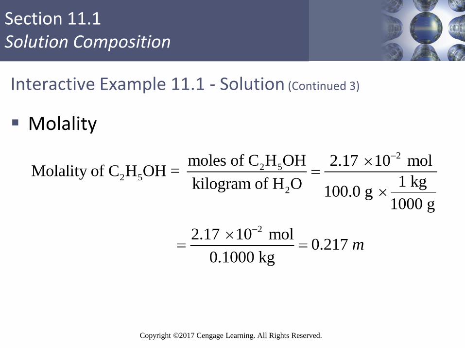
Interactive Example 11.1 - Solution (Continued 3)
Molality
2
2 52 5
2
moles of C H OH 2.17 10 molMolality of C H OH =
1 kgkilogram of H O100.0 g
1000 g
22.17 10 mol0.217
0.1000 kgm

Section 11.1 Solution Composition
Copyright ©2017 Cengage Learning. All Rights Reserved.
Critical Thinking
You are given two aqueous solutions with different ionic solutes (Solution A and Solution B)
What if you are told that Solution A has a greater concentration than Solution B by mass percent, but Solution B has a greater concentration than Solution A in terms of molality?
Is this possible? If not, explain why not
If it is possible, provide example solutes for A and B and justify your answer with calculations

Section 11.1 Solution Composition
Copyright ©2017 Cengage Learning. All Rights Reserved.
Normality (N)
Measure of concentration
Number of equivalents per liter of solution
Definition of an equivalent depends on the reaction that takes place in a solution
For acid–base reactions, the equivalent is the mass of acid or base that can accept or provide exactly 1 mole of protons
For oxidation–reduction reactions, the equivalent is the quantity of oxidizing or reducing agent that can accept or provide 1 mole of electrons

Section 11.1 Solution Composition
Copyright ©2017 Cengage Learning. All Rights Reserved.
Interactive Example 11.2 - Calculating Various Methods of Solution Composition from the Molarity
The electrolyte in automobile lead storage batteries is a 3.75 M sulfuric acid solution that has a density of 1.230 g/mL
Calculate the mass percent, molality, and normality of the sulfuric acid

Section 11.1 Solution Composition
Copyright ©2017 Cengage Learning. All Rights Reserved.
Interactive Example 11.2 - Solution
What is the density of the solution in grams per liter?
What mass of H2SO4 is present in 1.00 L of solution?
We know 1 liter of this solution contains 1230 g of the mixture of sulfuric acid and water
3g 1000 mL1.230 1.230 10 g/L
mL 1 L

Section 11.1 Solution Composition
Copyright ©2017 Cengage Learning. All Rights Reserved.
Interactive Example 11.2 - Solution (Continued 1)
Since the solution is 3.75 M, we know that 3.75 moles of H2SO4 is present per liter of solution
The number of grams of H2SO4 present is
2 4
2 4
98.0 g H SO3.75 mol 368 g H SO
1 mol

Section 11.1 Solution Composition
Copyright ©2017 Cengage Learning. All Rights Reserved.
Interactive Example 11.2 - Solution (Continued 2)
How much water is present in 1.00 L of solution?
The amount of water present in 1 liter of solution is obtained from the difference
What is the mass percent?
Since we now know the masses of the solute and solvent, we can calculate the mass percent
2 4 21230 g solution 368 g H SO = 862 g H O
Section 11.1 Solution Composition
Copyright ©2017 Cengage Learning. All Rights Reserved.
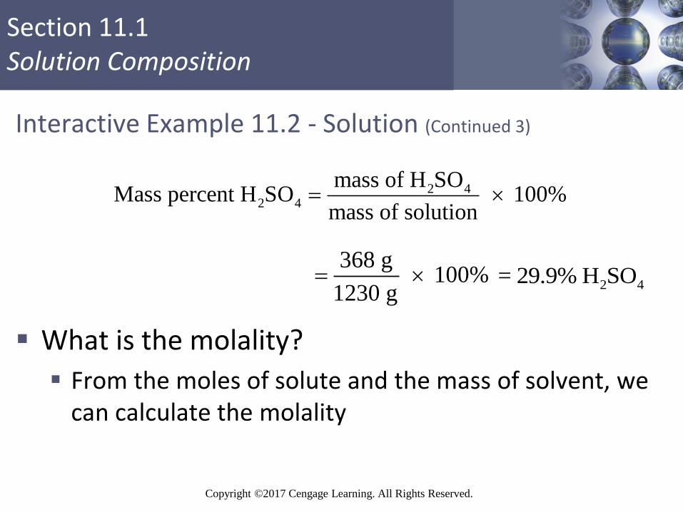
Interactive Example 11.2 - Solution (Continued 3)
What is the molality?
From the moles of solute and the mass of solvent, we can calculate the molality
2 42 4
mass of H SOMass percent H SO 100%
mass of solution
368 g 100%
1230 g
2 4= 29.9% H SO

Section 11.1 Solution Composition
Copyright ©2017 Cengage Learning. All Rights Reserved.
Interactive Example 11.2 - Solution (Continued 4)
2 42 4
2
moles H SOMolality of H SO
kilogram of H O
2 4
22
2
3.75 mol H SO4.35
1 kg H O862 g H O
1000 g H O
m

Section 11.1 Solution Composition
Copyright ©2017 Cengage Learning. All Rights Reserved.
Interactive Example 11.2 - Solution (Continued 5)
What is the normality?
Since each sulfuric acid molecule can furnish two protons, 1 mole of H2SO4 represents 2 equivalents
Thus, a solution with 3.75 moles of H2SO4 per liter contains 2×3.75 = 7.50 equivalents per liter
The normality is 7.50 N

Section 11.2 The Energies of Solution Formation
Copyright ©2017 Cengage Learning. All Rights Reserved.
Steps Involved in the Formation of a Liquid Solution
1. Expand the solute
Separate the solute into its individual components
2. Expand the solvent
Overcome intermolecular forces in the solvent to make room for the solute
3. Allow the solute and solvent to interact to form the solution
Copyright © Cengage Learning. All rights reserved 20

Section 11.2 The Energies of Solution Formation
Copyright ©2017 Cengage Learning. All Rights Reserved.
Steps Involved in the Formation of a Liquid Solution (Continued)
Steps 1 and 2 are endothermic
Forces must be overcome to expand the solute and solvent
Step 3 is often exothermic
Copyright © Cengage Learning. All rights reserved 21
Section 11.2 The Energies of Solution Formation
Copyright ©2017 Cengage Learning. All Rights Reserved.
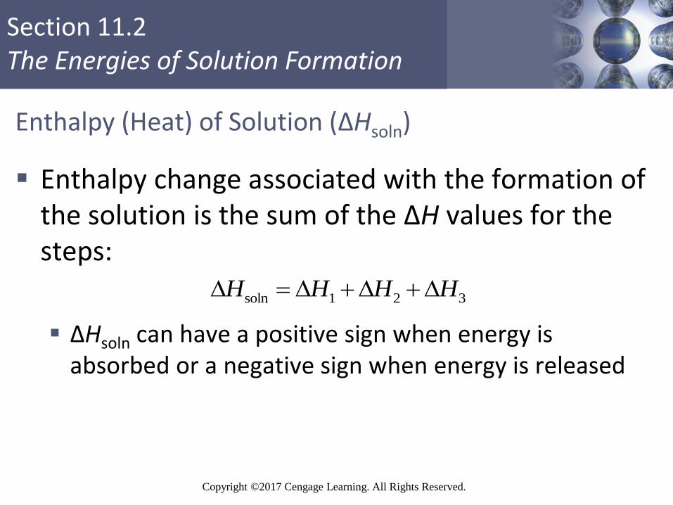
Enthalpy (Heat) of Solution (ΔHsoln)
Enthalpy change associated with the formation of the solution is the sum of the ΔH values for the steps:
ΔHsoln can have a positive sign when energy is absorbed or a negative sign when energy is released
Copyright © Cengage Learning. All rights reserved 22
soln 1 2 3H H H H

Section 11.2 The Energies of Solution Formation
Copyright ©2017 Cengage Learning. All Rights Reserved.
Figure 11.2 - The Heat of Solution
Copyright © Cengage Learning. All rights reserved 23

Section 11.2 The Energies of Solution Formation
Copyright ©2017 Cengage Learning. All Rights Reserved.
Factors That Favor a Process
Increase in probability of the mixed state when the solute and solvent are placed together
Processes that require large amounts of energy tend not to occur
Like dissolves like
Copyright © Cengage Learning. All rights reserved 24

Section 11.2 The Energies of Solution Formation
Copyright ©2017 Cengage Learning. All Rights Reserved.
Table 11.3 - The Energy Terms for Various Types of Solutes and Solvents

Section 11.2 The Energies of Solution Formation
Copyright ©2017 Cengage Learning. All Rights Reserved.
Critical Thinking
You and a friend are studying for a chemistry exam What if your friend tells you, “Since exothermic
processes are favored and the sign of the enthalpy change tells us whether or not a process is endothermic or exothermic, the sign of ΔHsoln tells us whether or not a solution will form”? How would you explain to your friend that this conclusion is
not correct? What part, if any, of what your friend says is correct?

Section 11.2 The Energies of Solution Formation
Copyright ©2017 Cengage Learning. All Rights Reserved.
Interactive Example 11.3 - Differentiating Solvent Properties
Decide whether liquid hexane (C6H14) or liquid methanol (CH3OH) is the more appropriate solvent for the substances grease (C20H42) and potassium iodide (KI)

Section 11.2 The Energies of Solution Formation
Copyright ©2017 Cengage Learning. All Rights Reserved.
Interactive Example 11.3 - Solution
Hexane is a nonpolar solvent because it contains C—H bonds
Hexane will work best for the nonpolar solute grease
Methanol has an O—H group that makes it significantly polar
Will serve as the better solvent for the ionic solid KI

Section 11.2 The Energies of Solution Formation
Copyright ©2017 Cengage Learning. All Rights Reserved.
Exercise
For each of the following pairs, predict which substance would be more soluble in water
NH3
CH3COOH

Section 11.3 Factors Affecting Solubility
Copyright ©2017 Cengage Learning. All Rights Reserved.
Structure Effects
Vitamins can be used to study the relationship among molecular structure, polarity, and solubility
Fat-soluble vitamins (A, D, E, and K) are nonpolar
Considered to be hydrophobic (water-fearing)
Can build up in the fatty tissues of the body
Water-soluble vitamins (B and C) are polar
Considered to be hydrophilic (water-loving)
Must be consumed regularly as they are excreted
Copyright © Cengage Learning. All rights reserved 30

Section 11.3 Factors Affecting Solubility
Copyright ©2017 Cengage Learning. All Rights Reserved.
Pressure Effects
Pressure increases the solubility of a gas
Henry’s law: Amount of a gas dissolved in a solution is directly proportional to the pressure of the gas above the solution
C - Concentration of the dissolved gas
k - Constant
P - Partial pressure of the gaseous solute above the solution
Copyright © Cengage Learning. All rights reserved 31
C kP

Section 11.3 Factors Affecting Solubility
Copyright ©2017 Cengage Learning. All Rights Reserved.
Figure 11.5 - Schematic Diagram That Depicts the Increase in Gas Solubility with Pressure
Copyright © Cengage Learning. All rights reserved 32

Section 11.3 Factors Affecting Solubility
Copyright ©2017 Cengage Learning. All Rights Reserved.
Interactive Example 11.4 - Calculations Using Henry’s Law
A certain soft drink is bottled so that a bottle at 25°C contains CO2 gas at a pressure of 5.0 atm over the liquid
Assuming that the partial pressure of CO2 in the atmosphere is 4.0×10⁻⁴ atm, calculate the equilibrium concentrations of CO2 in the soda both before and after the bottle is opened
The Henry’s law constant for CO2 in aqueous solution is 3.1×10⁻² mol/L · atm at 25°C

Section 11.3 Factors Affecting Solubility
Copyright ©2017 Cengage Learning. All Rights Reserved.
Interactive Example 11.4 - Solution
What is Henry’s law for CO2?
CCO2 = kCO2
PCO2
Where kCO2 = 3.1×10⁻² mol/L · atm
What is the CCO2 in the unopened bottle?
In the unopened bottle, PCO2 = 5.0 atm
2 2 2CO CO CO
2
=
= 3.1 10 mol/L atm 5.0 atm = 0.16 mol/L
C k P

Section 11.3 Factors Affecting Solubility
Copyright ©2017 Cengage Learning. All Rights Reserved.
Interactive Example 11.4 - Solution (Continued)
What is the CCO2 in the opened bottle?
In the opened bottle, the CO2 in the soda eventually reaches equilibrium with the atmospheric CO2, so PCO2
= 4.0×10⁻⁴ atm and
Note the large change in concentration of CO2
This is why soda goes “flat” after being open for a while
2 2 2
2 4
CO CO CO
5
mol = 3.1 10 4.0 10 atm
L atm
=1.2 10 mol/L
C k P

Section 11.3 Factors Affecting Solubility
Copyright ©2017 Cengage Learning. All Rights Reserved.
Temperature Effects (for Aqueous Solutions)
Solids dissolve rapidly at higher temperatures
Amount of solid that can be dissolved may increase or decrease with increasing temperature
Solubilities of some substances decrease with increasing temperature
Predicting temperature dependence of solubility is very difficult
Copyright © Cengage Learning. All rights reserved 36

Section 11.3 Factors Affecting Solubility
Copyright ©2017 Cengage Learning. All Rights Reserved.
Figure 11.7 - The Solubilities of Several Gases in Water
Copyright © Cengage Learning. All rights reserved 37

Section 11.3 Factors Affecting Solubility
Copyright ©2017 Cengage Learning. All Rights Reserved.
Temperature Effects (for Aqueous Solutions) (Continued)
Solubility of a gas in water decreases with increasing temperature
Water used for industrial cooling is returned to its natural source at higher than ambient temperatures
Causes thermal pollution
Warm water tends to float over the colder water, blocking oxygen absorption
Leads to the formation of boiler scale
Copyright © Cengage Learning. All rights reserved 38

Section 11.4 The Vapor Pressures of Solutions
Copyright ©2017 Cengage Learning. All Rights Reserved.
Figure 11.9 - An Aqueous Solution and Pure Water in a Closed Environment
Copyright © Cengage Learning. All rights reserved 39
Section 11.4 The Vapor Pressures of Solutions
Copyright ©2017 Cengage Learning. All Rights Reserved.
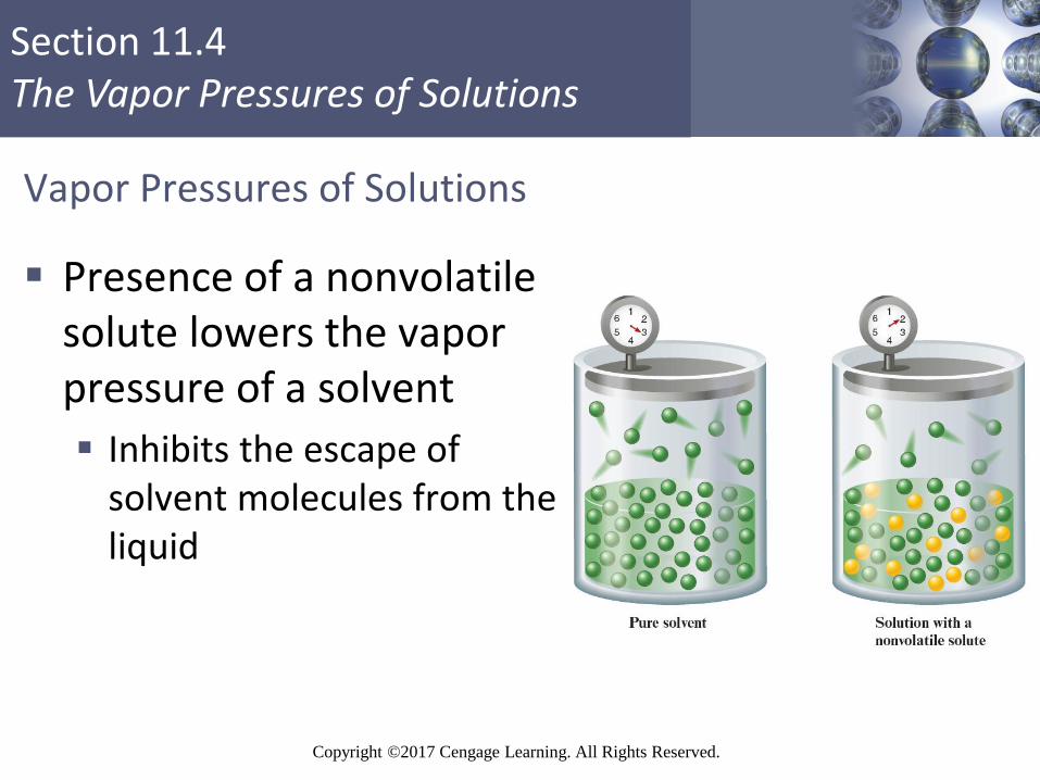
Vapor Pressures of Solutions
Presence of a nonvolatile solute lowers the vapor pressure of a solvent
Inhibits the escape of solvent molecules from the liquid
Copyright © Cengage Learning. All rights reserved 40

Section 11.4 The Vapor Pressures of Solutions
Copyright ©2017 Cengage Learning. All Rights Reserved.
Raoult's Law
Psoln - Observed vapor pressure of the solution
χsolvent - Mole fraction of the solvent
P0solvent - Vapor pressure of the pure solvent
Nonvolatile solute simply dilutes the solvent
Copyright © Cengage Learning. All rights reserved 41
0
soln solvent solventP P

Section 11.4 The Vapor Pressures of Solutions
Copyright ©2017 Cengage Learning. All Rights Reserved.
Graphical Representation of Raoult's Law
Can be represented as a linear equation of the form y = mx + b
y = Psoln
x = χsolvent
m = P0solvent
b = 0
Slope of the graph is a straight line with a slope equal to P0
solvent
Copyright © Cengage Learning. All rights reserved 42

Section 11.4 The Vapor Pressures of Solutions
Copyright ©2017 Cengage Learning. All Rights Reserved.
Figure 11.11 - Plot of Raoult's Law
Copyright © Cengage Learning. All rights reserved 43

Section 11.4 The Vapor Pressures of Solutions
Copyright ©2017 Cengage Learning. All Rights Reserved.
Interactive Example 11.5 - Calculating the Vapor Pressure of a Solution
Calculate the expected vapor pressure at 25°C for a solution prepared by dissolving 158.0 g common table sugar (sucrose, molar mass = 342.3 g/mol) in 643.5 cm3 of water
At 25°C, the density of water is 0.9971 g/cm3 and the vapor pressure is 23.76 torr

Section 11.4 The Vapor Pressures of Solutions
Copyright ©2017 Cengage Learning. All Rights Reserved.
Interactive Example 11.5 - Solution
What is Raoult’s law for this case?
To calculate the mole fraction of water in the solution, we must first determine the number of moles of sucrose and the moles of water present
2 2
0
soln H O H OP P

Section 11.4 The Vapor Pressures of Solutions
Copyright ©2017 Cengage Learning. All Rights Reserved.
Interactive Example 11.5 - Solution (Continued 1)
What are the moles of sucrose?
What are the moles of water?
To determine the moles of water present, we first convert volume to mass using the density:
3 22 23
2
0.9971 g H O643.5 cm H O 641.6 g H O
cm H O
1 mol sucroseMoles of sucrose 158.0 g sucrose 0.4616 mol sucrose
342.3 g sucrose

Section 11.4 The Vapor Pressures of Solutions
Copyright ©2017 Cengage Learning. All Rights Reserved.
Interactive Example 11.5 - Solution (Continued 2)
The number of moles of water
What is the mole fraction of water in the solution?
22 2
2
1 mol H O641.6 g H O 35.60 mol H O
18.02 g H O
2
2H O
2
mol H O 35.60 mol
mol H O + mol sucrose 35.60 mol + 0.4616 mol
35.60 mol0.9873
36.06 mol

Section 11.4 The Vapor Pressures of Solutions
Copyright ©2017 Cengage Learning. All Rights Reserved.
Interactive Example 11.5 - Solution (Continued 3)
The vapor pressure of the solution is:
The vapor pressure of water has been lowered from 23.76 torr in the pure state to 23.46 torr in the solution
The vapor pressure has been lowered by 0.30 torr
2 2
0
soln H O H OP P
0.9872 23.76 torr 23.46 torr

Section 11.4 The Vapor Pressures of Solutions
Copyright ©2017 Cengage Learning. All Rights Reserved.
Lowering of the Vapor Pressure
Helps in counting molecules
Provides a means to experimentally determine molar masses
Raoult’s law helps ascertain the number of moles of solute present in a solution
Helps characterize solutions
Provides valuable information about the nature of the solute after it dissolves

Section 11.4 The Vapor Pressures of Solutions
Copyright ©2017 Cengage Learning. All Rights Reserved.
Nonideal Solutions
Both components are volatile in liquid–liquid solutions
Contribute to the total vapor pressure
Modified Raoult’s law is applied here
PTOTAL - Total vapor pressure of a solution containing A and B
χA and χB - Mole fractions of A and B
Copyright © Cengage Learning. All rights reserved 50
0 0
TOTAL A B A A B B P P P P P

Section 11.4 The Vapor Pressures of Solutions
Copyright ©2017 Cengage Learning. All Rights Reserved.
Nonideal Solutions (Continued)
P0A and P0
B - Vapor pressures of pure A and pure B
PA and PB - Partial pressures resulting from molecules of A and of B in the vapor above the solution
Ideal solution: Liquid–liquid solution that obeys Raoult’s law
Nearly ideal behavior is observed when solute–solute, solvent–solvent, and solute–solvent interactions are similar
Copyright © Cengage Learning. All rights reserved 51

Section 11.4 The Vapor Pressures of Solutions
Copyright ©2017 Cengage Learning. All Rights Reserved.
Behavior of Various Types of Solutions
When ΔHsoln is large and negative:
Strong interactions exist between the solvent and solute
A negative deviation is expected from Raoult’s law
Both components have low escaping tendency in the solution than in pure liquids
Example - Acetone–water solution

Section 11.4 The Vapor Pressures of Solutions
Copyright ©2017 Cengage Learning. All Rights Reserved.
Behavior of Various Types of Solutions (Continued 1)
When ΔHsoln is positive (endothermic), solute–solvent interactions are weaker
Molecules in the solution have a higher tendency to escape, and there is positive deviation from Raoult’s law
Example - Solution of ethanol and hexane

Section 11.4 The Vapor Pressures of Solutions
Copyright ©2017 Cengage Learning. All Rights Reserved.
Behavior of Various Types of Solutions (Continued 2)
In a solution of very similar liquids:
ΔHsoln is close to zero
Solution closely obeys Raoult’s law
Example - Benzene and toluene

Section 11.4 The Vapor Pressures of Solutions
Copyright ©2017 Cengage Learning. All Rights Reserved.
Interactive Example 11.7 - Calculating the Vapor Pressure of a Solution Containing Two Liquids
A solution is prepared by mixing 5.81 g acetone (C3H6O, molar mass = 58.1 g/mol) and 11.9 g chloroform (HCCl3, molar mass = 119.4 g/mol)
At 35°C, this solution has a total vapor pressure of 260 torr
Is this an ideal solution?
The vapor pressures of pure acetone and pure chloroform at 35°C are 345 and 293 torr, respectively

Section 11.4 The Vapor Pressures of Solutions
Copyright ©2017 Cengage Learning. All Rights Reserved.
Interactive Example 11.7 - Solution
To decide whether this solution behaves ideally, we first calculate the expected vapor pressure using Raoult’s law:
A stands for acetone, and C stands for chloroform
The calculated value can then be compared with the observed vapor pressure
0 0
TOTAL A A C CP P P

Section 11.4 The Vapor Pressures of Solutions
Copyright ©2017 Cengage Learning. All Rights Reserved.
Interactive Example 11.7 - Solution (Continued 1)
First, we must calculate the number of moles of acetone and chloroform:
1 mol acetone5.81 g acetone 0.100 mol acetone
58.1 g acetone
1 mol chloroform11.9 g chloroform 0.100 mol chloroform
119 g chloroform

Section 11.4 The Vapor Pressures of Solutions
Copyright ©2017 Cengage Learning. All Rights Reserved.
Interactive Example 11.7 - Solution (Continued 2)
The solution contains equal numbers of moles of acetone and chloroform
χA = 0.500 and χC = 0.500
The expected vapor pressure is
Comparing this value with the observed pressure of 260 torr shows that the solution does not behave ideally
TOTAL 0.500 345 torr 0.500 293 torr 319 torrP

Section 11.4 The Vapor Pressures of Solutions
Copyright ©2017 Cengage Learning. All Rights Reserved.
Interactive Example 11.7 - Solution (Continued 3)
The observed value is lower than that expected
This negative deviation from Raoult’s law can be explained in terms of the hydrogen-bonding interaction which lowers the tendency of these molecules to escape from the solution

Section 11.5 Boiling-Point Elevation and Freezing-Point Depression
Copyright ©2017 Cengage Learning. All Rights Reserved.
Colligative Properties
Depend on the number of the solute particles in an ideal solution
Do not depend on the identity of the solute particles
Include boiling-point elevation, freezing-point depression, and osmotic pressure
Help determine:
The nature of a solute after it is dissolved in a solvent
The molar masses of substances
Copyright © Cengage Learning. All rights reserved 60

Section 11.5 Boiling-Point Elevation and Freezing-Point Depression
Copyright ©2017 Cengage Learning. All Rights Reserved.
Boiling-Point Elevation
Nonvolatile solute elevates the boiling point of the solvent
Magnitude of the boiling-point elevation depends on the concentration of the solute
Change in boiling point can be represented as follows:
ΔT - Boiling-point elevation
Kb - Molal boiling-point elevation constant
msolute - Molality of the solute
Copyright © Cengage Learning. All rights reserved 61
b soluteT K m

Section 11.5 Boiling-Point Elevation and Freezing-Point Depression
Copyright ©2017 Cengage Learning. All Rights Reserved.
Figure 11.14 - Phase Diagrams for Pure Water and for an Aqueous Solution Containing a Nonvolatile Solute
Copyright © Cengage Learning. All rights reserved 62

Section 11.5 Boiling-Point Elevation and Freezing-Point Depression
Copyright ©2017 Cengage Learning. All Rights Reserved.
Table 11.5 - Molal Boiling-Point Elevation Constants (Kb) and Freezing-Point Depression Constants (Kf) for Several Solvents
Section 11.5 Boiling-Point Elevation and Freezing-Point Depression
Copyright ©2017 Cengage Learning. All Rights Reserved.
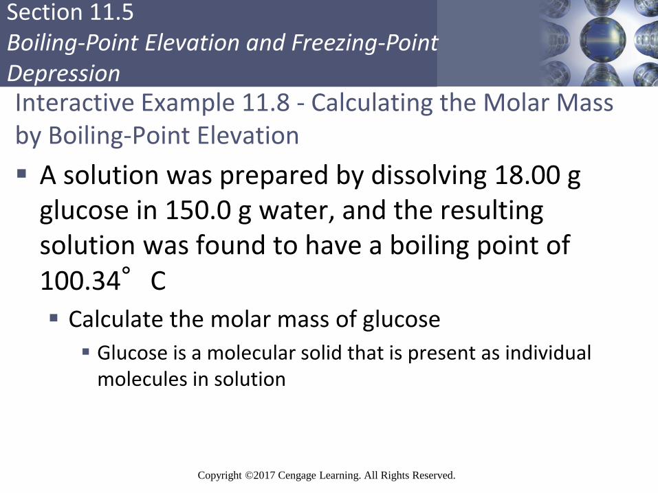
Interactive Example 11.8 - Calculating the Molar Mass by Boiling-Point Elevation
A solution was prepared by dissolving 18.00 g glucose in 150.0 g water, and the resulting solution was found to have a boiling point of 100.34°C
Calculate the molar mass of glucose
Glucose is a molecular solid that is present as individual molecules in solution

Section 11.5 Boiling-Point Elevation and Freezing-Point Depression
Copyright ©2017 Cengage Learning. All Rights Reserved.
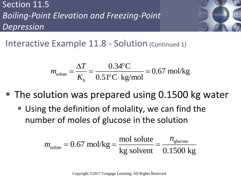
Interactive Example 11.8 - Solution
We make use of the following equation:
Where ΔT = 100.34°C – 100.00°C = 0.34°C
For water, Kb = 0.51
The molality of this solution then can be calculated by rearranging the boiling-point elevation equation
b soluteT K m
Section 11.5 Boiling-Point Elevation and Freezing-Point Depression
Copyright ©2017 Cengage Learning. All Rights Reserved.
Interactive Example 11.8 - Solution (Continued 1)
The solution was prepared using 0.1500 kg water
Using the definition of molality, we can find the number of moles of glucose in the solution
solute
b
0.34 C0.67 mol/kg
0.51 C kg/mol
Tm
K
glucose
solute
mol solute0.67 mol/kg
kg solvent 0.1500 kg
nm

Section 11.5 Boiling-Point Elevation and Freezing-Point Depression
Copyright ©2017 Cengage Learning. All Rights Reserved.
Interactive Example 11.8 - Solution (Continued 2)
Thus, 0.10 mole of glucose has a mass of 18.00 g, and 1.0 mole of glucose has a mass of 180 g (10×18.00 g)
The molar mass of glucose is 180 g/mol
glucose 0.67 mol/kg 0.1500 kg 0.10 moln

Section 11.5 Boiling-Point Elevation and Freezing-Point Depression
Copyright ©2017 Cengage Learning. All Rights Reserved.
Freezing-Point Depression
When a solute is dissolved in a solvent, the freezing point of the solution is lower than that of the pure solvent
Water in a solution has lower vapor pressure than that of pure ice
As the solution is cooled, the vapor pressure of ice and that of liquid water will become equal
Temperature at this point is below 0°C, and the freezing point has been depressed
Copyright © Cengage Learning. All rights reserved 68

Section 11.5 Boiling-Point Elevation and Freezing-Point Depression
Copyright ©2017 Cengage Learning. All Rights Reserved.
Figure 11.15 - Freezing-Point Depression: Model
Ice in equilibrium with liquid water
Ice in equilibrium with liquid water containing a dissolved
solute

Section 11.5 Boiling-Point Elevation and Freezing-Point Depression
Copyright ©2017 Cengage Learning. All Rights Reserved.
Equation for Freezing-Point Depression
ΔT - Freezing-point depression
Kf - Molal freezing-point depression constant
msolute - Molality of solute
Used to:
Ascertain molar masses
Characterize solutions
Copyright © Cengage Learning. All rights reserved 70
f soluteT K m

Section 11.5 Boiling-Point Elevation and Freezing-Point Depression
Copyright ©2017 Cengage Learning. All Rights Reserved.
Exercise
Calculate the freezing point and boiling point of an antifreeze solution that is 50.0% by mass of ethylene glycol (HOCH2CH2OH) in water
Ethylene glycol is a nonelectrolyte
Tf = 229.9°C
Tb = 108.2°C

Section 11.5 Boiling-Point Elevation and Freezing-Point Depression
Copyright ©2017 Cengage Learning. All Rights Reserved.
Interactive Example 11.10 - Determining Molar Mass by Freezing-Point Depression
A chemist is trying to identify a human hormone that controls metabolism by determining its molar mass
A sample weighing 0.546 g was dissolved in 15.0 g benzene, and the freezing-point depression was determined to be 0.240°C
Calculate the molar mass of the hormone

Section 11.5 Boiling-Point Elevation and Freezing-Point Depression
Copyright ©2017 Cengage Learning. All Rights Reserved.
Interactive Example 11.10 - Solution
Kf for benzene is 5.12°C · kg/mol, so the molality of the hormone is:
hormone
f
0.240°C
5.12°C kg/mol
Tm
K
24.69 10 mol/kg

Section 11.5 Boiling-Point Elevation and Freezing-Point Depression
Copyright ©2017 Cengage Learning. All Rights Reserved.
Interactive Example 11.10 - Solution (Continued 1)
The moles of hormone can be obtained from the definition of molality:
Or
2
solute
mol hormone4.69 10 mol/kg =
0.0150 kg benzene
m
2 4molmol hormone 4.69 10 0.0150 kg 7.04 10 mol
kg

Section 11.5 Boiling-Point Elevation and Freezing-Point Depression
Copyright ©2017 Cengage Learning. All Rights Reserved.
Interactive Example 11.10 - Solution (Continued 2)
Since 0.546 g hormone was dissolved, 7.04×10⁻⁴ mole of hormone has a mass of 0.546 g, and
Thus, the molar mass of the hormone is 776 g/mol
4
0.546 g
7.04 10 mol 1.00 mol
x
776x

Section 11.6 Osmotic Pressure
Copyright ©2017 Cengage Learning. All Rights Reserved.
Osmosis
Flow of solvent into solution through a semipermeable membrane
Semipermeable membrane: Permits solvent but not solute molecules to pass through
Osmotic pressure: Result of increased hydrostatic pressure on the solution than on the pure solvent
Caused by the difference in levels of the liquids at equilibrium
Copyright © Cengage Learning. All rights reserved 76

Section 11.6 Osmotic Pressure
Copyright ©2017 Cengage Learning. All Rights Reserved.
Figure 11.16 - Process of Osmosis

Section 11.6 Osmotic Pressure
Copyright ©2017 Cengage Learning. All Rights Reserved.
Preventing Osmosis
Apply pressure to the solution
Minimum pressure that stops the osmosis is equal to the osmotic pressure of the solution

Section 11.6 Osmotic Pressure
Copyright ©2017 Cengage Learning. All Rights Reserved.
Uses of Osmotic Pressure
Characterize solutions
Determine molar masses
A small concentration of solute produces a relatively large osmotic pressure

Section 11.6 Osmotic Pressure
Copyright ©2017 Cengage Learning. All Rights Reserved.
Understanding Osmotic Pressure
Equation that represents the dependence of osmotic pressure on solution concentration
Π - Osmotic pressure in atmospheres
M - Molarity of the solution
R - Gas law constant
T - Kelvin temperature
MRT

Section 11.6 Osmotic Pressure
Copyright ©2017 Cengage Learning. All Rights Reserved.
Critical Thinking
Consider the following model of osmotic pressure:

Section 11.6 Osmotic Pressure
Copyright ©2017 Cengage Learning. All Rights Reserved.
Critical Thinking (Continued)
What if both sides contained a different pure solvent, each with a different vapor pressure?
What would the system look like at equilibrium?
Assume the different solvent molecules are able to pass through the membrane

Section 11.6 Osmotic Pressure
Copyright ©2017 Cengage Learning. All Rights Reserved.
Interactive Example 11.11 - Determining Molar Mass from Osmotic Pressure
To determine the molar mass of a certain protein, 1.00×10⁻³ g of it was dissolved in enough water to make 1.00 mL of solution
The osmotic pressure of this solution was found to be 1.12 torr at 25.0°C
Calculate the molar mass of the protein

Section 11.6 Osmotic Pressure
Copyright ©2017 Cengage Learning. All Rights Reserved.
Interactive Example 11.11 - Solution
We use the following equation:
In this case we have:
R = 0.08206 L · atm/K · mol
T = 25.0 + 273 = 298 K
MRT
31 atm1.12 torr 1.47 10 atm
760 torr

Section 11.6 Osmotic Pressure
Copyright ©2017 Cengage Learning. All Rights Reserved.
Interactive Example 11.11 - Solution (Continued 1)
Note that the osmotic pressure must be converted to atmospheres because of the units of R
Solving for M gives
351.47 10 atm
6.01 10 mol/L0.08206 L atm/K mol 298 K
M

Section 11.6 Osmotic Pressure
Copyright ©2017 Cengage Learning. All Rights Reserved.
Interactive Example 11.11 - Solution (Continued 2)
Since 1.00×10⁻³ g protein was dissolved in 1 mL solution, the mass of protein per liter of solution is 1.00 g
The solution’s concentration is 6.01×10⁻⁵ mol/L
This concentration is produced from 1.00×10⁻³ g protein per milliliter, or 1.00 g/L
Thus 6.01×10⁻⁵ mol protein has a mass of 1.00 g

Section 11.6 Osmotic Pressure
Copyright ©2017 Cengage Learning. All Rights Reserved.
Interactive Example 11.11 - Solution (Continued 3)
The molar mass of the protein is 1.66×10⁴ g/mol
This molar mass may seem very large, but it is relatively small for a protein
5
1.00 g
6.01 10 mol 1.00 mol
x
41.66 10 g x

Section 11.6 Osmotic Pressure
Copyright ©2017 Cengage Learning. All Rights Reserved.
Dialysis
Occurs at the walls of most animal and plant cells
Membranes permit the transfer of:
Solvent molecules
Small solute molecules and ions
Application
Use of artificial kidney machines to purify blood

Section 11.6 Osmotic Pressure
Copyright ©2017 Cengage Learning. All Rights Reserved.
Isotonic, Hypertonic, and Hypotonic Solutions
Isotonic solutions: Solutions with identical osmotic pressures
Intravenously administered fluids must be isotonic with body fluids
Hypertonic solutions - Have osmotic pressure higher than that of the cell fluids
Hypotonic solutions - Have osmotic pressure lower than that of the cell fluids

Section 11.6 Osmotic Pressure
Copyright ©2017 Cengage Learning. All Rights Reserved.
Red Blood Cells (RBCs) and Osmosis
RBCs in a hypertonic solution undergo crenation
Shrivel up as water moves out of the cells

Section 11.6 Osmotic Pressure
Copyright ©2017 Cengage Learning. All Rights Reserved.
Red Blood Cells (RBCs) and Osmosis (Continued)
RBCs in a hypotonic solution undergo hemolysis
Swell up and rupture as excess water flows into the cells

Section 11.7 Colligative Properties of Electrolyte Solutions
Copyright ©2017 Cengage Learning. All Rights Reserved.
Interactive Example 11.12 - Isotonic Solutions
What concentration of sodium chloride in water is needed to produce an aqueous solution isotonic with blood (Π = 7.70 atm at 25°C)?

Section 11.7 Colligative Properties of Electrolyte Solutions
Copyright ©2017 Cengage Learning. All Rights Reserved.
Interactive Example 11.12 - Solution
We can calculate the molarity of the solute from the following equation:
This represents the total molarity of solute particles
or MRT M =RT
7.70 atm
0.315 mol/L0.08206 L atm/K mol 298 K
M

Section 11.7 Colligative Properties of Electrolyte Solutions
Copyright ©2017 Cengage Learning. All Rights Reserved.
Interactive Example 11.12 - Solution (Continued)
NaCl gives two ions per formula unit
Therefore, the concentration of NaCl needed is
0.315 0.1575 0.158
2
MM M
+NaCl Na + Cl
0.1575 M 0.1575 M 0.1575 M
0.315 M

Section 11.7 Colligative Properties of Electrolyte Solutions
Copyright ©2017 Cengage Learning. All Rights Reserved.
Reverse Osmosis
Results when a solution in contact with a pure solvent across a semipermeable membrane is subjected to an external pressure larger than its osmotic pressure
Pressure will cause a net flow of solvent from the solution to the solvent
Semipermeable membrane acts as a molecular filter
Removes solute particles

Section 11.7 Colligative Properties of Electrolyte Solutions
Copyright ©2017 Cengage Learning. All Rights Reserved.
Figure 11.20 - Reverse Osmosis

Section 11.7 Colligative Properties of Electrolyte Solutions
Copyright ©2017 Cengage Learning. All Rights Reserved.
Desalination
Removal of dissolved salts from a solution

Section 11.7 Colligative Properties of Electrolyte Solutions
Copyright ©2017 Cengage Learning. All Rights Reserved.
van’t Hoff Factor, i
Provides the relationship between the moles of solute dissolved and the moles of particles in solution
Expected value for i can be calculated for a salt by noting the number of ions per formula unit
Copyright © Cengage Learning. All rights reserved 98
moles of particles in solution
moles of solute dissolvedi

Section 11.7 Colligative Properties of Electrolyte Solutions
Copyright ©2017 Cengage Learning. All Rights Reserved.
Ion Pairing
Oppositely charged ions aggregate and behave as a single particle
Occurs in solutions
Example
Sodium and chloride ions in NaCl
Copyright © Cengage Learning. All rights reserved 99

Section 11.7 Colligative Properties of Electrolyte Solutions
Copyright ©2017 Cengage Learning. All Rights Reserved.
Ion Pairing (Continued)
Essential in concentrated solutions
As the solution becomes more dilute, ions are spread apart leading to less ion pairing
Occurs in all electrolyte solutions to some extent
Deviation of i from the expected value is the greatest when ions have multiple charges
Ion pairing is important for highly charged ions
Copyright © Cengage Learning. All rights reserved 100
Section 11.7 Colligative Properties of Electrolyte Solutions
Copyright ©2017 Cengage Learning. All Rights Reserved.
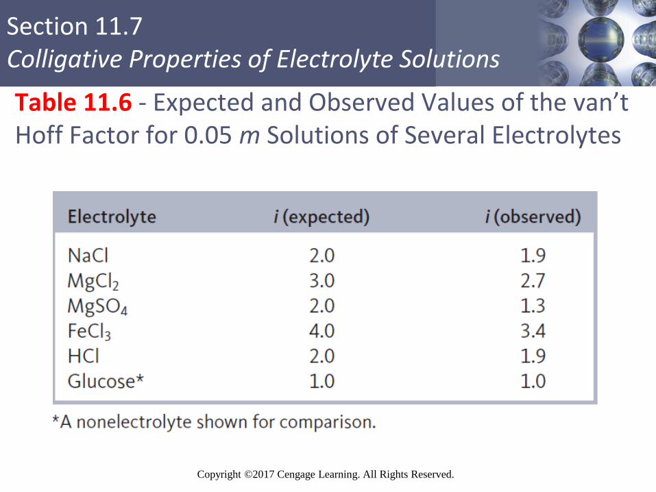
Table 11.6 - Expected and Observed Values of the van’t Hoff Factor for 0.05 m Solutions of Several Electrolytes

Section 11.7 Colligative Properties of Electrolyte Solutions
Copyright ©2017 Cengage Learning. All Rights Reserved.
Ion Pairing in Electrolyte Solutions
Colligative properties are given by including the van’t Hoff factor in the necessary equation
For changes in freezing and boiling points
K - Freezing-point depression or boiling-point elevation
constant for the solvent
For osmotic pressure
T imK
iMRT

Section 11.7 Colligative Properties of Electrolyte Solutions
Copyright ©2017 Cengage Learning. All Rights Reserved.
Interactive Example 11.13 - Osmotic Pressure
The observed osmotic pressure for a 0.10 M solution of Fe(NH4)2(SO4)2 at 25°C is 10.8 atm
Compare the expected and experimental values for i

Section 11.7 Colligative Properties of Electrolyte Solutions
Copyright ©2017 Cengage Learning. All Rights Reserved.
Interactive Example 11.13 - Solution
The ionic solid Fe(NH4)2(SO4)2 dissociates in water to produce 5 ions:
Thus, the expected value for i is 5
2H O 2+ 2
4 4 4 42 2Fe NH SO Fe + 2NH 2SO

Section 11.7 Colligative Properties of Electrolyte Solutions
Copyright ©2017 Cengage Learning. All Rights Reserved.
Interactive Example 11.13 - Solution (Continued 1)
We can obtain the experimental value for i by using the equation for osmotic pressure:
Π = 10.8 atm
M = 0.10 mol/L
R = 0.08206 L · atm/K · mol
T = 25 + 273 = 298 K
or iMRT iMRT

Section 11.7 Colligative Properties of Electrolyte Solutions
Copyright ©2017 Cengage Learning. All Rights Reserved.
Interactive Example 11.13 - Solution (Continued 2)
Substituting these values into the equation gives:
The experimental value for i is less than the expected value, presumably because of ion pairing
iMRT
10.8 atm
0.10 mol/L 0.08206 L atm/K mol 298 K
4.4i

Section 11.8 Colloids
Copyright ©2017 Cengage Learning. All Rights Reserved.
The Tyndall Effect
Scattering of light by particles
Used to distinguish between a suspension and a true solution
When a beam of intense light is projected:
The beam is visible from the side in a suspension Light is scattered by suspended particles
The light beam is invisible is in a true solution Individual ions and molecules dispersed in the solution are too small
to scatter visible light
Copyright © Cengage Learning. All rights reserved 107

Section 11.8 Colloids
Copyright ©2017 Cengage Learning. All Rights Reserved.
Figure 11.23 - The Tyndall Effect

Section 11.8 Colloids
Copyright ©2017 Cengage Learning. All Rights Reserved.
Colloidal Dispersion or Colloids
Suspension of tiny particles in some medium
Can be either single large molecules or aggregates of molecules or ions ranging in size from 1 to 1000 nm
Classified according to the states of the dispersed phase and the dispersing medium
Copyright © Cengage Learning. All rights reserved 109

Section 11.8 Colloids
Copyright ©2017 Cengage Learning. All Rights Reserved.
Table 11.7 - Types of Colloids

Section 11.8 Colloids
Copyright ©2017 Cengage Learning. All Rights Reserved.
Stabilizing Colloids
Major factor - Electrostatic repulsions
A colloid is electrically neutral
Each center particle is surrounded by a layer of positive ions, with negative ions in the outer layer
When placed in an electric field, the center attracts from the medium a layer of ions, all of the same charge
Outer layer contains ions with the same charge that repel each other

Section 11.8 Colloids
Copyright ©2017 Cengage Learning. All Rights Reserved.
Coagulation
Destruction of a colloid
Heating increases the velocities of the particles causing them to collide
Ion barriers are penetrated, and the particles can aggregate
Repetition of the process enables the particle to settle out
Adding an electrolyte neutralizes the adsorbed ion layers
Copyright © Cengage Learning. All rights reserved 112

Section 11.8 Colloids
Copyright ©2017 Cengage Learning. All Rights Reserved.
Examples of Coagulation
Colloidal clay particles in seawater coagulate due to high salt content
Removal of soot from smoke
The suspended particles are removed when smoke is passed through an electrostatic precipitator