Chapter 1 The CLP Procedure (Experimental)support.sas.com/publishing/pubcat/chaps/59309.pdf ·...

Chapter 1The CLP Procedure (Experimental)

Chapter Contents

OVERVIEW . . . . . . . . . . . . . . . . . . . . . . . . . . . . . . . . . . . 7The Constraint Satisfaction Problem. . . . . . . . . . . . . . . . . . . . . 7Techniques for Solving CSPs. . . . . . . . . . . . . . . . . . . . . . . . . 8The CLP Procedure. . . . . . . . . . . . . . . . . . . . . . . . . . . . . . 9

INTRODUCTORY EXAMPLES . . . . . . . . . . . . . . . . . . . . . . . . 11Send More Money. . . . . . . . . . . . . . . . . . . . . . . . . . . . . . .11Eight Queens. . . . . . . . . . . . . . . . . . . . . . . . . . . . . . . . . .11

SYNTAX . . . . . . . . . . . . . . . . . . . . . . . . . . . . . . . . . . . . .13Functional Summary. . . . . . . . . . . . . . . . . . . . . . . . . . . . . .14PROC CLP Statement. . . . . . . . . . . . . . . . . . . . . . . . . . . . .15ACTIVITY Statement . . . . . . . . . . . . . . . . . . . . . . . . . . . . .17ALLDIFF Statement. . . . . . . . . . . . . . . . . . . . . . . . . . . . . .18ARRAY Statement. . . . . . . . . . . . . . . . . . . . . . . . . . . . . . .19FOREACH Statement. . . . . . . . . . . . . . . . . . . . . . . . . . . . .19LINCON Statement. . . . . . . . . . . . . . . . . . . . . . . . . . . . . .19REIFY Statement . . . . . . . . . . . . . . . . . . . . . . . . . . . . . . .20REQUIRES Statement. . . . . . . . . . . . . . . . . . . . . . . . . . . . .21RESOURCE Statement. . . . . . . . . . . . . . . . . . . . . . . . . . . .21SCHEDULE Statement. . . . . . . . . . . . . . . . . . . . . . . . . . . .22VAR Statement . . . . . . . . . . . . . . . . . . . . . . . . . . . . . . . .23

DETAILS . . . . . . . . . . . . . . . . . . . . . . . . . . . . . . . . . . . . .24Modes of Operation. . . . . . . . . . . . . . . . . . . . . . . . . . . . . .24Activity Data Set. . . . . . . . . . . . . . . . . . . . . . . . . . . . . . . .24Schedule Data Set. . . . . . . . . . . . . . . . . . . . . . . . . . . . . . .26Constraint Data Set. . . . . . . . . . . . . . . . . . . . . . . . . . . . . .27Solution Data Set . . . . . . . . . . . . . . . . . . . . . . . . . . . . . . .28

REFERENCES . . . . . . . . . . . . . . . . . . . . . . . . . . . . . . . . . .29

6 � Chapter 1. The CLP Procedure (Experimental)

Chapter 1The CLP Procedure (Experimental)

Overview

The CLP procedure is a finite domain constraint programming solver for constraintsatisfaction problems (CSPs) with linear, logical, global, and scheduling constraints.In addition to having an expressive syntax for representing CSPs, the solver fea-tures powerful built-in consistency routines and constraint propagation algorithms,a choice of nondeterministic search strategies, and controls for guiding the searchmechanism that enable you to solve a diverse array of combinatorial problems.

For the most recent updates to the documentation for this experimental pro-cedure, see the Statistics and Operations Research Documentation page athttp://support.sas.com/rnd/app/doc.html.

The Constraint Satisfaction Problem

Many important problems in areas such as Artificial Intelligence (AI) and OperationsResearch (OR) can be formulated as constraint satisfaction problems. A CSP is de-fined by a finite set of variables taking values from finite domains and a finite set ofconstraints restricting the values the variables can simultaneously take.

More formally, a CSP can be defined as a triple〈X, D,C〉 where

• X = {x1, . . . , xn} is a finite set ofvariables.

• D = {D1, . . . , Dn} is a finite set ofdomains, whereDi is a finite set of possi-ble values that the variablexi can take.Di is known as thedomainof variablexi.

• C = {c1, . . . , cm} is a finite set ofconstraintsrestricting the values that thevariables can simultaneously take.

Note that the domains need not represent consecutive integers. For example, thedomain of a variable could be the set of allevennumbers in the interval [0, 100]. Adomain does not even need to be totally numeric. In fact, in a scheduling problemwith resources, the values are typically multidimensional. For example, an activitycan be considered as a variable and each element of the domain would be ann-tuplethat represents a start time for the activity as well as the resource(s) that must beassigned to the activity corresponding to the start time.

A solution to a CSP is an assignment of values to the variables in order to satisfy allthe constraints, and the problem amounts to finding solution(s), or possibly determin-ing that a solution does not exist.


The CLP procedure can be used to find one or more (and in some instances, all) so-lutions to a CSP with linear, logical, global, and scheduling constraints. The numericcomponents of all variable domains are assumed to be integers.

Techniques for Solving CSPs

Several techniques for solving CSPs are available.Kumar(1992) andTsang(1993)present a good overview of these techniques.

It should be noted that the Satisfiability problem (SAT) (Garey and Johnson1979) canbe regarded as a CSP. Consequently, most problems in this class are NP-completeproblems, and a backtracking search is an important technique for solving them(Floyd 1967). However, a backtracking approach is not very efficient due to thelate detection of conflicts; that is, it is oriented towardrecoveringfrom failures andnot avoidingthem to begin with. The search space is reduced only after detection ofa failure, and the performance of this technique drastically reduces with increasingproblem size.

Constraint Propagation

A more efficient technique is that of constraint propagation, which uses consistencytechniques to effectively prune the domains of variables. Consistency techniques arealso known as relaxation algorithms (Tsang1993) and the process is also referredto as problem reduction, domain filtering, or pruning. The research on consistencytechniques originated with the Waltz filtering algorithm (Waltz 1975). Constraintpropagation is characterized by the extent of propagation (also referred to as the levelof consistency) and the domain pruning scheme that is followed — domain prop-agation or interval propagation. In practice, interval propagation is preferred overdomain propagation due to its lower computational costs. This mechanism is dis-cussed in detail inVan Hentenryck(1989). However, constraint propagation is not acomplete solution technique and needs to be complemented by a search technique toensure success (Kumar1992).

Finite Domain Constraint Programming

Finite domain constraint programming is an effective and complete solution tech-nique that embeds incomplete constraint propagation techniques into a nondetermin-istic backtracking search mechanism, implemented as follows. Whenever a node isvisited, constraint propagation is carried out to attain a desired level of consistency. Ifthe domain of each variable reduces to a singleton set, the node represents a solutionto the CSP. If the domain of a variable becomes empty, the node is pruned. Otherwisea variable is selected, its domain distributed, and a new set of CSPs generated, eachof which is a child node of the current node. Several factors play a role in determin-ing the outcome of this mechanism, such as the extent of propagation (or level ofconsistency enforced), the variable selection strategy, and the variable assignment ordomain distribution strategy.

For example, the lack of any propagation reduces this technique to a simple gener-ate and test, whereas performing consistency on variables already selected reducesthis to chronological backtracking, one of the systematic search techniques. These

The CLP Procedure � 9

are also known as look-back schemas as they share the disadvantage of late conflictdetection. Look-ahead schemas, on the other hand, work to prevent future conflicts.Some popular examples of look-ahead strategies in increasing degree of consistencylevel are Forward Checking (FC), Partial Look Ahead (PLA), and Full Look Ahead(LA) (Kumar 1992). Forward Checking enforces consistency between the currentvariable and future variables; PLA and LA extend this even further to pairs of not yetinstantiated variables.

Two important consequences of this technique are that inconsistencies are discoveredearly on and that the current set of alternatives coherent with the existing partialsolution is dynamically maintained. These consequences are powerful enough toprune large parts of the search tree, thereby reducing the “combinatorial explosion”of the search process. However, although constraint propagation at each node resultsin fewer nodes in the search tree, the processing at each node is more expensive.The ideal scenario is to strike a balance between the extent of propagation and thesubsequent computation cost.

Variable selection is another strategy that can affect the solution process. The order inwhich variables are chosen for instantiation can have substantial impact on the com-plexity of the backtrack search. Several heuristics have been developed and analyzedfor selecting variable ordering. One of the more common ones is a dynamic heuristicbased on thefail first principle (Haralick and Elliot1980), which selects the vari-able whose domain has minimal size. Subsequent analysis of this heuristic by severalresearchers has validated this technique as providing substantial improvement for asignificant class of problems. Another popular technique is to instantiate the mostconstrained variable first. Both these strategies are based on the principle of selectingthe variable most likely to fail and to detect such failures as early as possible.

The domain distribution strategy for a selected variable is yet another area that caninfluence the performance of a backtracking search. However, good value orderingheuristics are expected to be very problem-specific (Kumar1992).

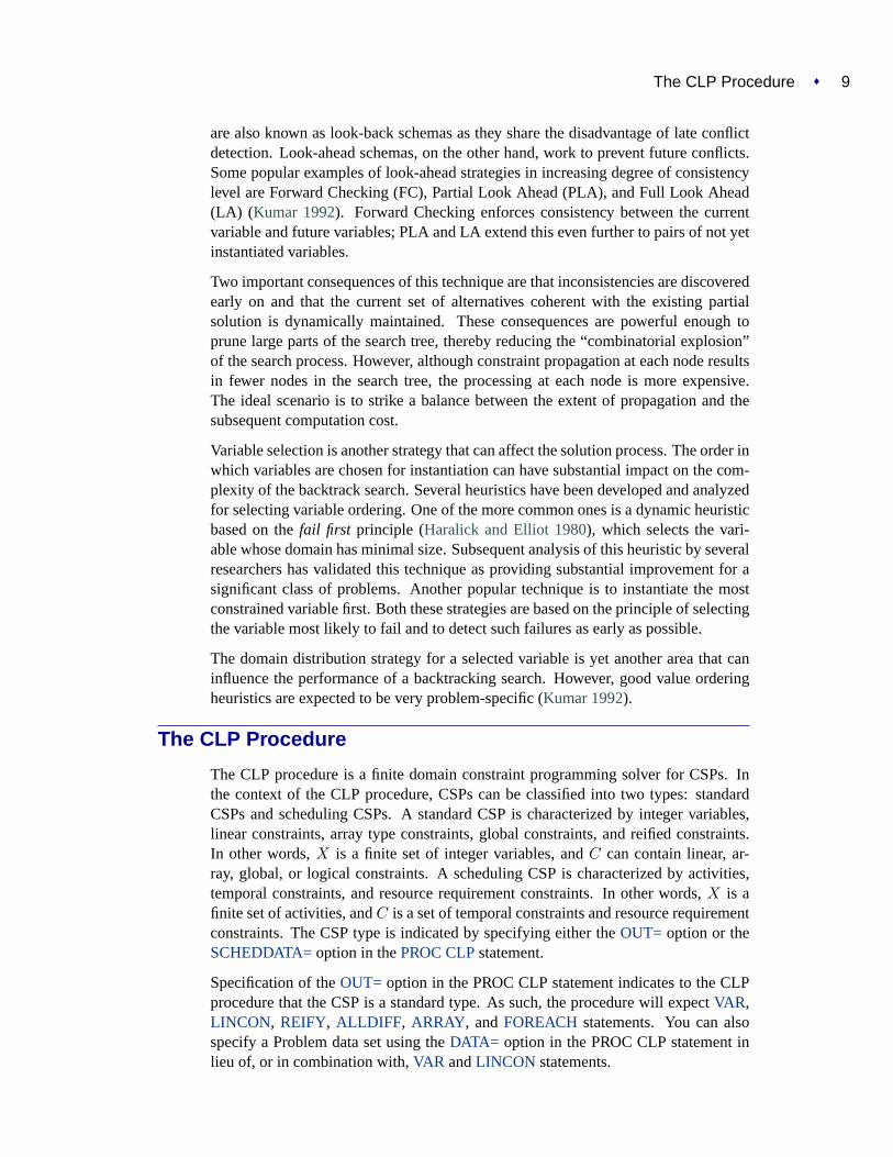
The CLP Procedure

The CLP procedure is a finite domain constraint programming solver for CSPs. Inthe context of the CLP procedure, CSPs can be classified into two types: standardCSPs and scheduling CSPs. A standard CSP is characterized by integer variables,linear constraints, array type constraints, global constraints, and reified constraints.In other words,X is a finite set of integer variables, andC can contain linear, ar-ray, global, or logical constraints. A scheduling CSP is characterized by activities,temporal constraints, and resource requirement constraints. In other words,X is afinite set of activities, andC is a set of temporal constraints and resource requirementconstraints. The CSP type is indicated by specifying either theOUT= option or theSCHEDDATA=option in thePROC CLPstatement.

Specification of theOUT= option in the PROC CLP statement indicates to the CLPprocedure that the CSP is a standard type. As such, the procedure will expectVAR,LINCON, REIFY, ALLDIFF, ARRAY, andFOREACHstatements. You can alsospecify a Problem data set using theDATA= option in the PROC CLP statement inlieu of, or in combination with,VAR andLINCON statements.


Specification of theSCHEDDATA= option in the PROC CLP statement indicates tothe CLP procedure that the CSP is a scheduling type. As such, the procedure willexpectACTIVITY , RESOURCE, REQUIRES, andSCHEDULE statements. Youcan also specify an Activity data set using theACTDATA= option in the PROC CLPstatement in lieu of, or in combination with, theACTIVITY andLINCON statements.Precedence relationships between activities must be defined using theACTDATA=data set. Resource requirements of activities must be defined using theRESOURCEandREQUIRESstatements.

The output data set contains any solutions determined by the CLP procedure. Formore information on the format and layout, see the“Details” section on page 24.

Consistency Techniques

The CLP procedure features a Full Look-Ahead algorithm for standard CSPs thatfollows a strategy of maintaining a version of Generalized Arc Consistency thatis based on the AC-3 Consistency routine (Mackworth1977). This strategy main-tains consistency between the selected variable and the unassigned variables and alsomaintains consistency between unassigned variables. For the scheduling CSPs, theCLP procedure uses a Forward Checking algorithm, an arc-consistency routine formaintaining consistency between unassigned activities, and energetic-based reason-ing methods for resource-constrained scheduling that feature the Edge Finder algo-rithm (Applegate and Cook1991). You can elect to turn off some of these consistencytechniques in the interest of performance.

Selection Strategy

A search algorithm for CSPs searches systematically through the possible assign-ments of values to variables. The order in which a variable is selected can be basedon astaticordering, which is determined before the search begins, or on adynamicordering, in which the choice of the next variable depends on the current state of thesearch. TheVARSELECT=option in the PROC CLP statement defines the variableselection strategy for a standard CSP. The default strategy is the dynamic MINR strat-egy, which selects the variable with the smallest range. TheACTSELECT=optionin theSCHEDULEstatement defines the activity selection strategy for a schedulingCSP. The default strategy is the RAND strategy, which selects an activity at randomfrom the set of activities that begin prior to the earliest early finish time. This strategywas proposed byNuijten (1994).

Assignment Strategy

Once a variable or an activity has been selected, the assignment strategy dictates thevalue that is assigned to it. For variables, the assignment strategy is specified with theVARASSIGN=option in the PROC CLP statement. The default assignment strategyselects the minimum value from the domain of the selected variable. For activities, theassignment strategy is specified with theACTASSIGN=option in theSCHEDULEstatement. The default strategy of RAND assigns the time to the earliest start time,and the resources are chosen randomly from the set of resource assignments thatsupport the selected start time.

Eight Queens � 11

Introductory Examples

The following examples illustrate the formulation and solution of two well-knownlogical puzzles in the constraint programming community using the CLP procedure.

Send More Money

The Send More Money problem consists of finding unique digits for the letters D, E,M, N, O, R, S, and Y such that S and M are different from zero (no leading zeros)and the equation

SEND + MORE = MONEY

is satisfied. The unique solution of the problem is9567 + 1085 = 10652.

UsingPROC CLP, we can solve this problem as follows:

proc clp dom=[0,9] /* Define the default domain */out=out; /* Name the output data set */

var S E N D M O R E M O N E Y;/* Declare the variables */lincon /* Linear constraints */

/* SEND + MORE = MONEY */1000*S + 100*E + 10*N + D + 1000*M + 100*O + 10*R + E=10000*M + 1000*O + 100*N + 10*E + Y,S<>0, /* No leading zeros */M<>0;

alldiff(); /* All variables have pairwise distinct values*/run;

Obs S E N D M O R Y

1 9 5 6 7 1 0 8 2

Figure 1.1. Solution to SEND + MORE = MONEY

Eight Queens

The Eight Queens problem is a special instance of theN -Queens problem where theobjective is to positionN queens on anN × N chessboard such that no two queensattack each other. The CLP procedure provides an expressive constraint for variablearrays that can be used for solving this problem very efficiently.

Since each queen must occupy a distinct row, we can model this using a variable arrayA of dimensionN , whereA[i] is the row number of the queen in columni. Sinceno two queens can be on the same row, it follows that all theA[i]’s must be pairwisedistinct.


In order to ensure that no two queens can be on the same diagonal, we must have thefollowing for all i andj:

A[j]−A[i] <> j − i

and

A[j]−A[i] <> i− j

In other words,

A[i]− i <> A[j]− j

and

A[i] + i <> A[j] + j

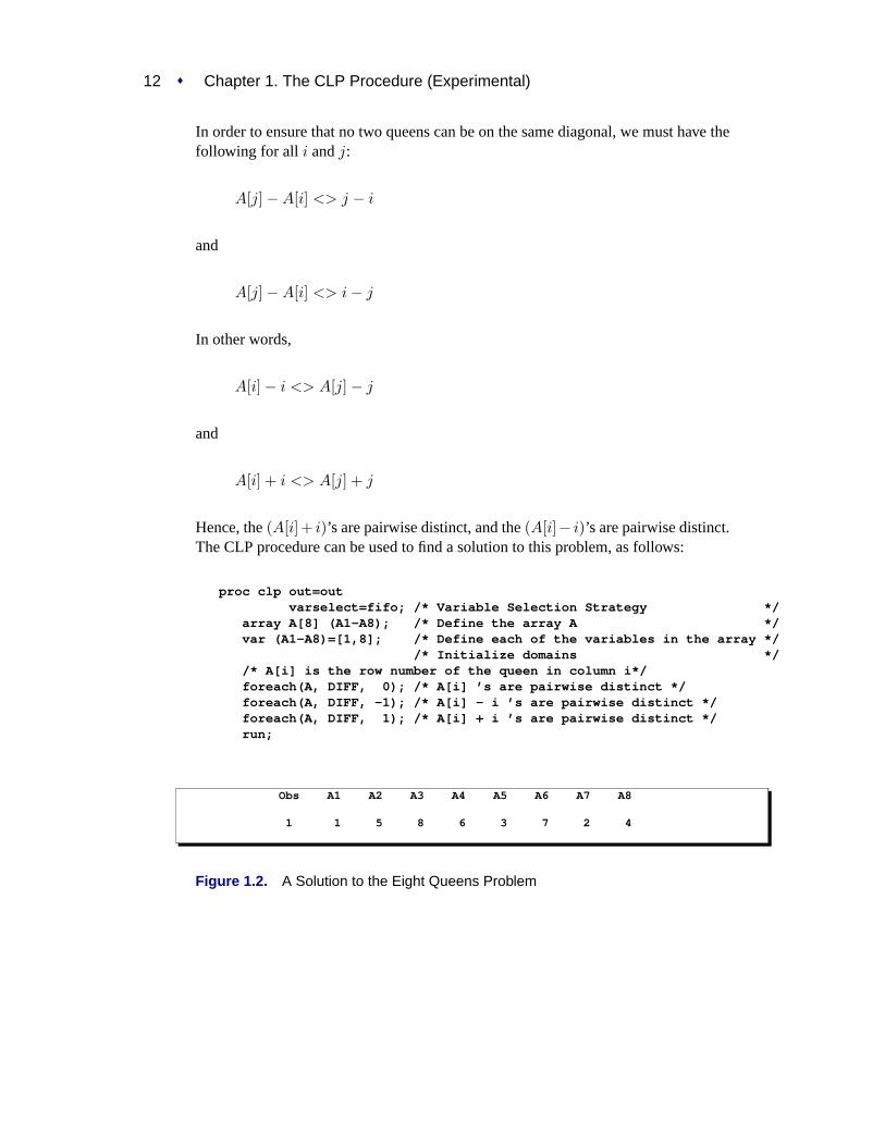
Hence, the(A[i]+ i)’s are pairwise distinct, and the(A[i]− i)’s are pairwise distinct.The CLP procedure can be used to find a solution to this problem, as follows:

proc clp out=outvarselect=fifo; /* Variable Selection Strategy */

array A[8] (A1-A8); /* Define the array A */var (A1-A8)=[1,8]; /* Define each of the variables in the array */

/* Initialize domains *//* A[i] is the row number of the queen in column i*/foreach(A, DIFF, 0); /* A[i] ’s are pairwise distinct */foreach(A, DIFF, -1); /* A[i] - i ’s are pairwise distinct */foreach(A, DIFF, 1); /* A[i] + i ’s are pairwise distinct */run;

Obs A1 A2 A3 A4 A5 A6 A7 A8

1 1 5 8 6 3 7 2 4

Figure 1.2. A Solution to the Eight Queens Problem

Syntax � 13

Figure 1.3. A Solution to the Eight Queens Problem

Syntax

The following statements are used in PROC CLP:

PROC CLP options ;ACTIVITY activity specifications ;ALLDIFF alldiff constraints ;ARRAY array specifications ;FOREACH foreach constraints ;LINCON linear constraints ;REIFY reified constraints ;REQUIRES resource requirement constraints ;RESOURCE resource specifications ;SCHEDULE schedule options ;VAR variable specifications ;


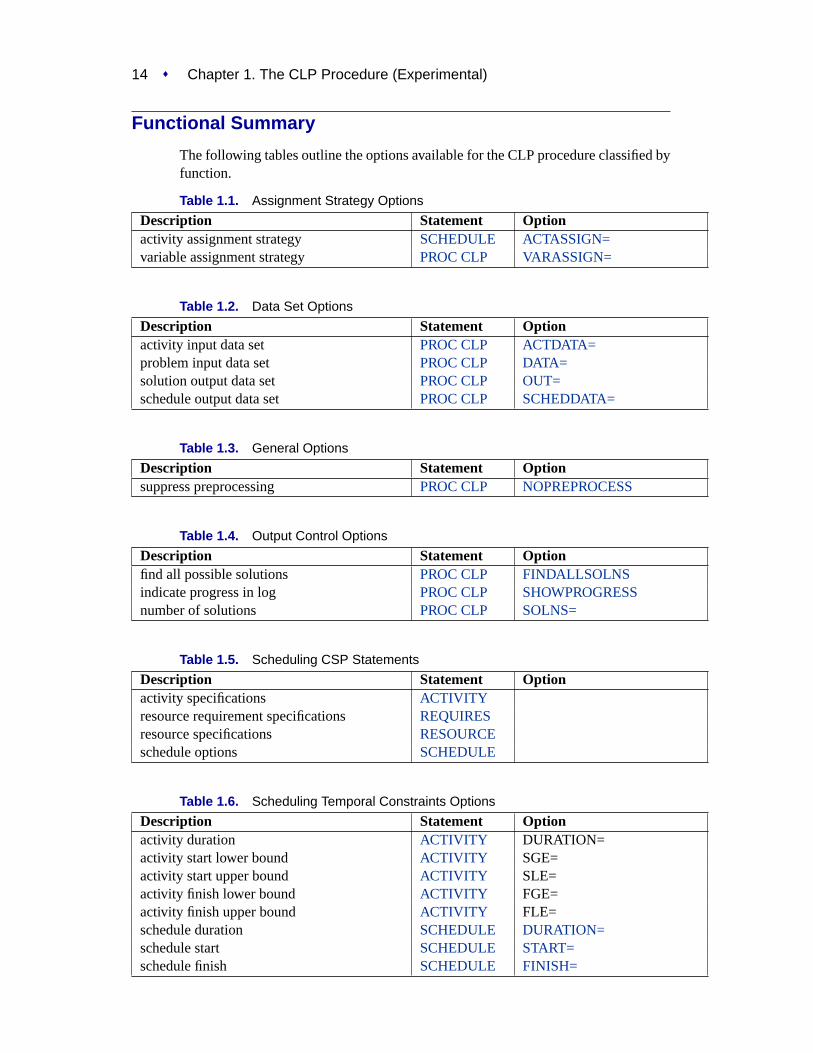
Functional Summary

The following tables outline the options available for the CLP procedure classified byfunction.

Table 1.1. Assignment Strategy Options

Description Statement Optionactivity assignment strategy SCHEDULE ACTASSIGN=variable assignment strategy PROC CLP VARASSIGN=

Table 1.2. Data Set Options

Description Statement Optionactivity input data set PROC CLP ACTDATA=problem input data set PROC CLP DATA=solution output data set PROC CLP OUT=schedule output data set PROC CLP SCHEDDATA=

Table 1.3. General Options

Description Statement Optionsuppress preprocessing PROC CLP NOPREPROCESS

Table 1.4. Output Control Options

Description Statement Optionfind all possible solutions PROC CLP FINDALLSOLNSindicate progress in log PROC CLP SHOWPROGRESSnumber of solutions PROC CLP SOLNS=

Table 1.5. Scheduling CSP Statements

Description Statement Optionactivity specifications ACTIVITYresource requirement specifications REQUIRESresource specifications RESOURCEschedule options SCHEDULE

Table 1.6. Scheduling Temporal Constraints Options

Description Statement Optionactivity duration ACTIVITY DURATION=activity start lower bound ACTIVITY SGE=activity start upper bound ACTIVITY SLE=activity finish lower bound ACTIVITY FGE=activity finish upper bound ACTIVITY FLE=schedule duration SCHEDULE DURATION=schedule start SCHEDULE START=schedule finish SCHEDULE FINISH=

PROC CLP Statement � 15

Table 1.7. Scheduling Search Control Options

Description Statement Optiondeadend multiplier PROC CLP DEM=number of allowable deadends per restart PROC CLP DEPR=number of search restarts PROC CLP RESTARTS=edge finder consistency routine SCHEDULE EF

Table 1.8. Selection Strategy Options

Description Statement Optionactivity selection strategy SCHEDULE ACTSELECT=variable selection strategy PROC CLP VARSELECT=

Table 1.9. Standard CSP Statements

Description Statement Optionalldifferent constraints ALLDIFFarray specifications ARRAYforeach constraints FOREACHlinear constraints LINCONreified constraints REIFYvariable specifications VAR

PROC CLP StatementPROC CLP options ;

The following options can appear in the PROC CLP statement.

ACTDATA= SAS-data-setACTIVITY=SAS-data-set

identifies the input data set that defines the activities and temporal constraints. Thetemporal constraints consist of time alignment type constraints and precedence typeconstraints. The format of the ACTDATA= data set is similar to the Activity data setused by the CPM procedure in SAS/OR software. The activities and time alignmentconstraints can also be directly specified using theACTIVITY statement withoutthe need for a data set. The CLP procedure enables you to define activities using acombination of the two specifications.

DATA=SAS-data-setidentifies the input data set that defines the linear constraints. The format of theDATA= data set is similar to that used by the LP procedure in SAS/OR software.The linear constraints can also be specified inline using theLINCON statement. TheCLP procedure enables you to define linear constraints using a combination of thetwo specifications. When defining linear constraints, you must define the structuralvariables using aVAR statement.

DEM=dspecifies the deadend multiplier for the CSP. The deadend multiplier is used to deter-mine the number of deadends that are permitted before triggering a complete restart


of the search technique in a scheduling environment. The number of deadends isthe product of the deadend multiplier and the number of unassigned activities. Thedefault value is 0.15. This option is valid only with theSCHEDDATA=option.

DEPR=nspecifies the number of deadends that are permitted before PROC CLP restarts orterminates the search, depending on whether or not a randomized search strategy isused. In the case of a nonrandomized strategy,n is an upper bound on the number ofallowable deadends before terminating. In the case of a randomized strategy,n is anupper bound on the number of allowable deadends before restarting the search. TheDEPR= option has priority over theDEM= option. The default value of the DEPR=option is∞.

DOMAIN=[ lb, ub]DOM=[lb, ub]

specifies the global domain of all variables to be the closed interval [lb, ub]. You canoverride the global domain for a variable with aVAR statement or theDATA= dataset.

FINDALLSOLNSALLSOLNSFASFINDALL

attempts to find all possible solutions to the CSP. When a randomized search strat-egy is used, it is possible to rediscover the same solution and end up with multipleinstances of the same solution. This is currently the case when solving scheduling-related problems. Therefore, this option is ignored when solving a scheduling-relatedproblem.

NOPREPROCESSsuppresses any preprocessing that would typically be performed for the problem.

OUT=SAS-data-setidentifies the output data set that contains the solution(s) to the CSP, if any exist. Eachobservation in the OUT= data set corresponds to a solution of the CSP. The numberof solutions generated can be controlled using theSOLNS=option in thePROC CLPstatement.

RESTARTS=nspecifies the number of restarts of the randomized search technique before terminat-ing the procedure. The default value is 3.

SCHEDDATA=SAS-data-setSCHEDULE=SAS-data-set

identifies the output data set that contains the scheduling-related solution to the CSP,if one exists. Each observation in the SCHEDDATA= data set corresponds to anactivity. The format of the schedule data set is similar to the schedule data set gener-ated by the CPM and PM procedures in SAS/OR software. The number of solutionsgenerated can be controlled using theSOLNS=option in thePROC CLPstatement.

ACTIVITY Statement � 17

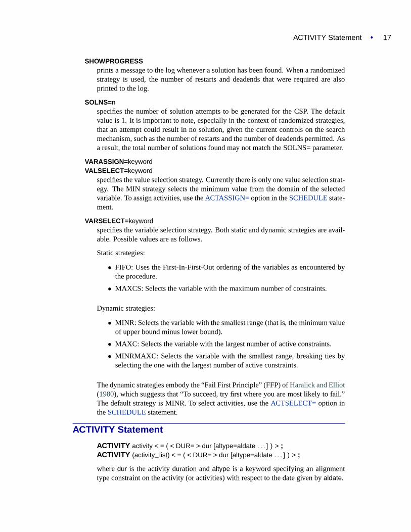
SHOWPROGRESSprints a message to the log whenever a solution has been found. When a randomizedstrategy is used, the number of restarts and deadends that were required are alsoprinted to the log.

SOLNS=nspecifies the number of solution attempts to be generated for the CSP. The defaultvalue is 1. It is important to note, especially in the context of randomized strategies,that an attempt could result in no solution, given the current controls on the searchmechanism, such as the number of restarts and the number of deadends permitted. Asa result, the total number of solutions found may not match the SOLNS= parameter.

VARASSIGN=keywordVALSELECT= keyword

specifies the value selection strategy. Currently there is only one value selection strat-egy. The MIN strategy selects the minimum value from the domain of the selectedvariable. To assign activities, use theACTASSIGN=option in theSCHEDULEstate-ment.

VARSELECT=keywordspecifies the variable selection strategy. Both static and dynamic strategies are avail-able. Possible values are as follows.

Static strategies:

• FIFO: Uses the First-In-First-Out ordering of the variables as encountered bythe procedure.

• MAXCS: Selects the variable with the maximum number of constraints.

Dynamic strategies:

• MINR: Selects the variable with the smallest range (that is, the minimum valueof upper bound minus lower bound).

• MAXC: Selects the variable with the largest number of active constraints.

• MINRMAXC: Selects the variable with the smallest range, breaking ties byselecting the one with the largest number of active constraints.

The dynamic strategies embody the “Fail First Principle” (FFP) ofHaralick and Elliot(1980), which suggests that “To succeed, try first where you are most likely to fail.”The default strategy is MINR. To select activities, use theACTSELECT=option intheSCHEDULEstatement.

ACTIVITY Statement

ACTIVITY activity < = ( < DUR= > dur [altype=aldate . . . ] ) > ;ACTIVITY (activity–list) < = ( < DUR= > dur [altype=aldate . . . ] ) > ;

wheredur is the activity duration andaltype is a keyword specifying an alignmenttype constraint on the activity (or activities) with respect to the date given byaldate.


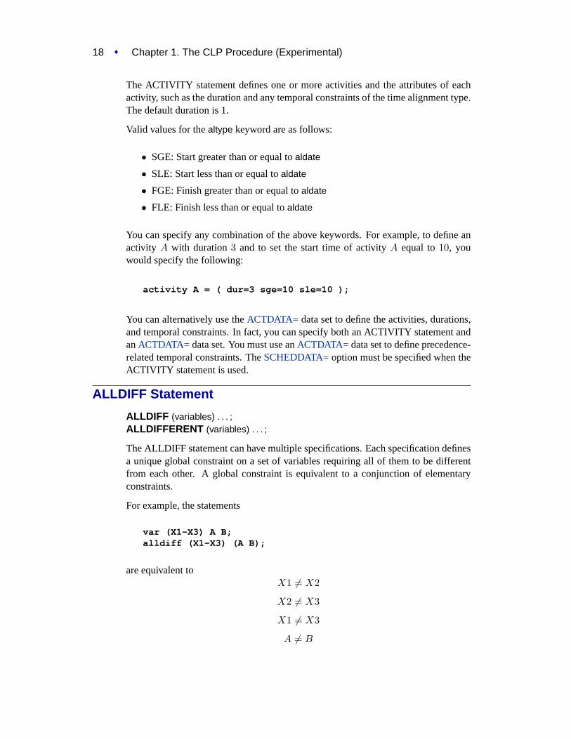
The ACTIVITY statement defines one or more activities and the attributes of eachactivity, such as the duration and any temporal constraints of the time alignment type.The default duration is 1.

Valid values for thealtype keyword are as follows:

• SGE: Start greater than or equal toaldate

• SLE: Start less than or equal toaldate

• FGE: Finish greater than or equal toaldate

• FLE: Finish less than or equal toaldate

You can specify any combination of the above keywords. For example, to define anactivity A with duration3 and to set the start time of activityA equal to10, youwould specify the following:

activity A = ( dur=3 sge=10 sle=10 );

You can alternatively use theACTDATA= data set to define the activities, durations,and temporal constraints. In fact, you can specify both an ACTIVITY statement andanACTDATA= data set. You must use anACTDATA= data set to define precedence-related temporal constraints. TheSCHEDDATA=option must be specified when theACTIVITY statement is used.

ALLDIFF Statement

ALLDIFF (variables) . . . ;ALLDIFFERENT (variables) . . . ;

The ALLDIFF statement can have multiple specifications. Each specification definesa unique global constraint on a set of variables requiring all of them to be differentfrom each other. A global constraint is equivalent to a conjunction of elementaryconstraints.

For example, the statements

var (X1-X3) A B;alldiff (X1-X3) (A B);

are equivalent toX1 6= X2

X2 6= X3

X1 6= X3

A 6= B

LINCON Statement � 19

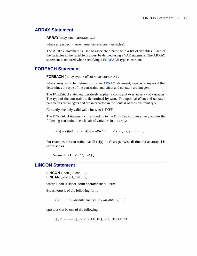
ARRAY Statement

ARRAY arrayspec [, arrayspec...];

wherearrayspec := arrayname [dimensions] (variables);

The ARRAY statement is used to associate a name with a list of variables. Each ofthe variables in the variable list must be defined using aVAR statement. The ARRAYstatement is required when specifying aFOREACHtype constraint.

FOREACH Statement

FOREACH ( array, type, <offset <, constant > > ) ;

wherearray must be defined using anARRAY statement,type is a keyword thatdetermines the type of the constraint, andoffset andconstant are integers.

The FOREACH statement iteratively applies a constraint over an array of variables.The type of the constraint is determined bytype. The optionaloffset andconstantparameters are integers and are interpreted in the context of the constraint type.

Currently, the only valid value fortype is DIFF.

The FOREACH statement corresponding to the DIFF keyword iteratively applies thefollowing constraint to each pair of variables in the array:

A[i] + offset× i 6= A[j] + offset× j ∀ i 6= j, i, j = 1, . . . ,m

For example, the constraint that all(A[i]− i)’s are pairwise distinct for an arrayA isexpressed as

foreach (A, diff, -1);

LINCON Statement

LINCON l–con [, l–con . . . ];LINEAR l–con [, l–con . . . ];

wherel–con := linear–term operator linear–term

linear–term is of the following form:

((< +|− > variable|number< ∗variable>) . . .)

operator can be one of the following:

≤, <, =,==,≥, >, <>, LE,EQ,GE,LT,GT,NE


The LINCON statement allows for a very general specification of linear constraints.In particular, it allows for specification of the following types of equality or inequalityconstraints:

n∑j=1

aijxj {≤ | < | = | ≥ | > | 6=} bi for i = 1, . . . ,m

For example, the constraint4x1 − 3x2 = 5 is expressed as

var x1 x2;lincon 4 * x1 - 3 * x2 = 5;

and the constraints10x1 − x2 ≥ 10

x1 + 5x2 6= 15

are expressed as

var x1 x2;lincon 10 <= 10 * x1 - x2,

x1 + 5 * x2 <> 15;

Note that variables can be specified on either side of an equality or inequality in aLINCON statement. Linear constraints can also be specified using theDATA= dataset. When using a LINCON statement, you must define the variables using aVARstatement.

REIFY Statement

REIFY variable : (l–con)...;

wherel–con := linear–term operator linear–term

linear–term is of the following form:

((< +|− > variable|number< ∗variable>) . . .)

operator can be one of the following:

≤, <, =,==,≥, >, <>, LE,EQ,GE,LT,GT,NE

The REIFY statement associates a binary variable with a linear constraint. The valueof the binary variable is 1 or 0 depending on whether the linear constraint is satisfiedor not, respectively. The linear constraint has been reified, and the logical variable isreferred to as the control variable. As with the other variables, the control variablemust also be defined in aVAR statement or in theDATA= data set.

RESOURCE Statement � 21

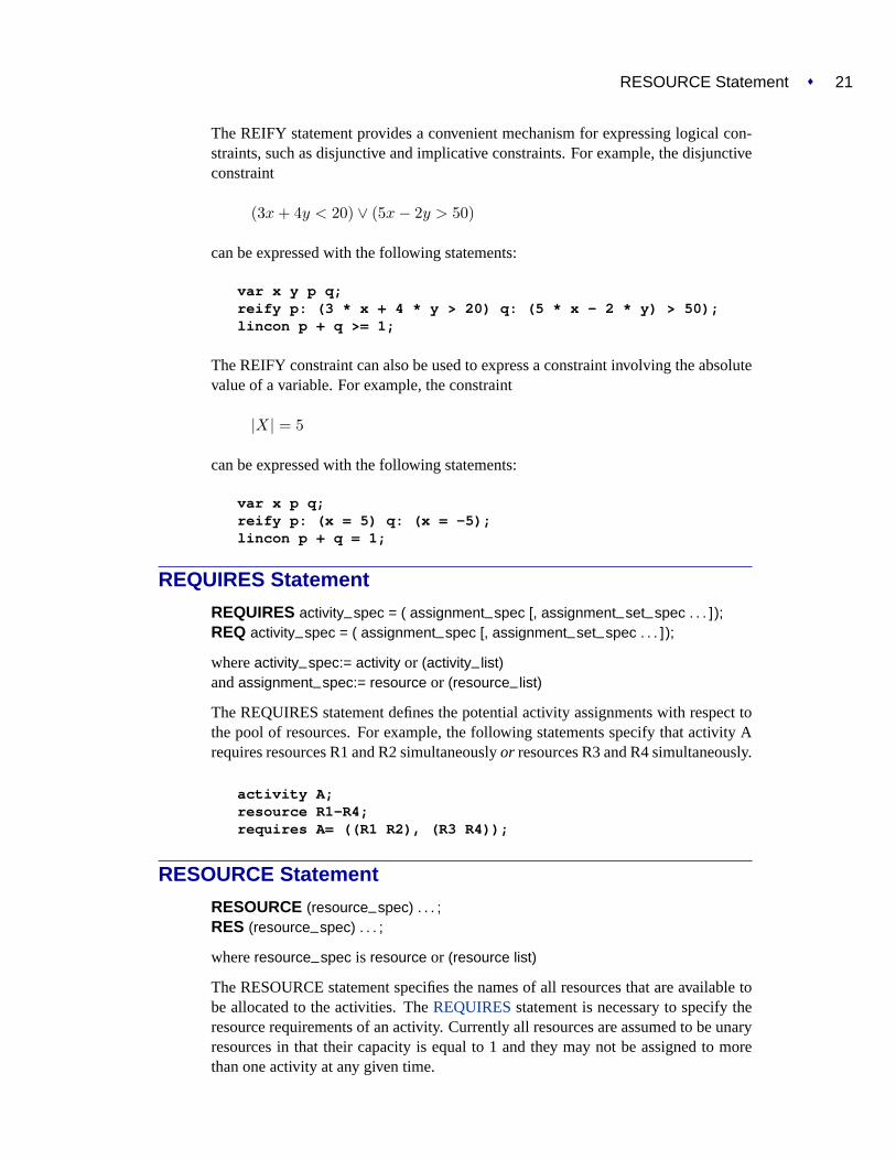
The REIFY statement provides a convenient mechanism for expressing logical con-straints, such as disjunctive and implicative constraints. For example, the disjunctiveconstraint

(3x + 4y < 20) ∨ (5x− 2y > 50)

can be expressed with the following statements:

var x y p q;reify p: (3 * x + 4 * y > 20) q: (5 * x - 2 * y) > 50);lincon p + q >= 1;

The REIFY constraint can also be used to express a constraint involving the absolutevalue of a variable. For example, the constraint

|X| = 5

can be expressed with the following statements:

var x p q;reify p: (x = 5) q: (x = -5);lincon p + q = 1;

REQUIRES Statement

REQUIRES activity–spec = ( assignment–spec [, assignment–set–spec . . . ]);REQ activity–spec = ( assignment–spec [, assignment–set–spec . . . ]);

whereactivity–spec:= activity or (activity–list)andassignment–spec:= resource or (resource–list)

The REQUIRES statement defines the potential activity assignments with respect tothe pool of resources. For example, the following statements specify that activity Arequires resources R1 and R2 simultaneouslyor resources R3 and R4 simultaneously.

activity A;resource R1-R4;requires A= ((R1 R2), (R3 R4));

RESOURCE Statement

RESOURCE (resource–spec) . . . ;RES (resource–spec) . . . ;

whereresource–spec is resource or (resource list)

The RESOURCE statement specifies the names of all resources that are available tobe allocated to the activities. TheREQUIRESstatement is necessary to specify theresource requirements of an activity. Currently all resources are assumed to be unaryresources in that their capacity is equal to 1 and they may not be assigned to morethan one activity at any given time.


SCHEDULE Statement

SCHEDULE options;

The following options can appear in the SCHEDULE statement.

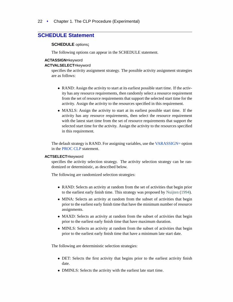
ACTASSIGN=keywordACTVALSELECT= keyword

specifies the activity assignment strategy. The possible activity assignment strategiesare as follows:

• RAND: Assign the activity to start at its earliest possible start time. If the activ-ity has any resource requirements, then randomly select a resource requirementfrom the set of resource requirements that support the selected start time for theactivity. Assign the activity to the resources specified in this requirement.

• MAXLS: Assign the activity to start at its earliest possible start time. If theactivity has any resource requirements, then select the resource requirementwith the latest start time from the set of resource requirements that support theselected start time for the activity. Assign the activity to the resources specifiedin this requirement.

The default strategy is RAND. For assigning variables, use theVARASSIGN=optionin thePROC CLPstatement.

ACTSELECT=keywordspecifies the activity selection strategy. The activity selection strategy can be ran-domized or deterministic, as described below.

The following are randomized selection strategies:

• RAND: Selects an activity at random from the set of activities that begin priorto the earliest early finish time. This strategy was proposed byNuijten (1994).

• MINA: Selects an activity at random from the subset of activities that beginprior to the earliest early finish time that have the minimum number of resourceassignments.

• MAXD: Selects an activity at random from the subset of activities that beginprior to the earliest early finish time that have maximum duration.

• MINLS: Selects an activity at random from the subset of activities that beginprior to the earliest early finish time that have a minimum late start date.

The following are deterministic selection strategies:

• DET: Selects the first activity that begins prior to the earliest activity finishdate.

• DMINLS: Selects the activity with the earliest late start time.

VAR Statement � 23

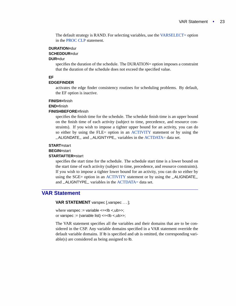
The default strategy is RAND. For selecting variables, use theVARSELECT=optionin thePROC CLPstatement.

DURATION=durSCHEDDUR=durDUR=dur

specifies the duration of the schedule. The DURATION= option imposes a constraintthat the duration of the schedule does not exceed the specified value.

EFEDGEFINDER

activates the edge finder consistency routines for scheduling problems. By default,the EF option is inactive.

FINISH=finishEND=finishFINISHBEFORE=finish

specifies the finish time for the schedule. The schedule finish time is an upper boundon the finish time of each activity (subject to time, precedence, and resource con-straints). If you wish to impose a tighter upper bound for an activity, you can doso either by using the FLE= option in anACTIVITY statement or by using the

–ALIGNDATE– and–ALIGNTYPE– variables in theACTDATA= data set.

START=startBEGIN=startSTARTAFTER=start

specifies the start time for the schedule. The schedule start time is a lower bound onthe start time of each activity (subject to time, precedence, and resource constraints).If you wish to impose a tighter lower bound for an activity, you can do so either byusing the SGE= option in anACTIVITY statement or by using the–ALIGNDATE–and–ALIGNTYPE– variables in theACTDATA= data set.

VAR Statement

VAR STATEMENT varspec [,varspec . . . ];

wherevarspec := variable <=<lb <,ub>>;or varspec := (variable list) <=<lb <,ub>>;

The VAR statement specifies all the variables and their domains that are to be con-sidered in the CSP. Any variable domains specified in a VAR statement override thedefault variable domains. Iflb is specified andub is omitted, the corresponding vari-able(s) are considered as being assigned tolb.


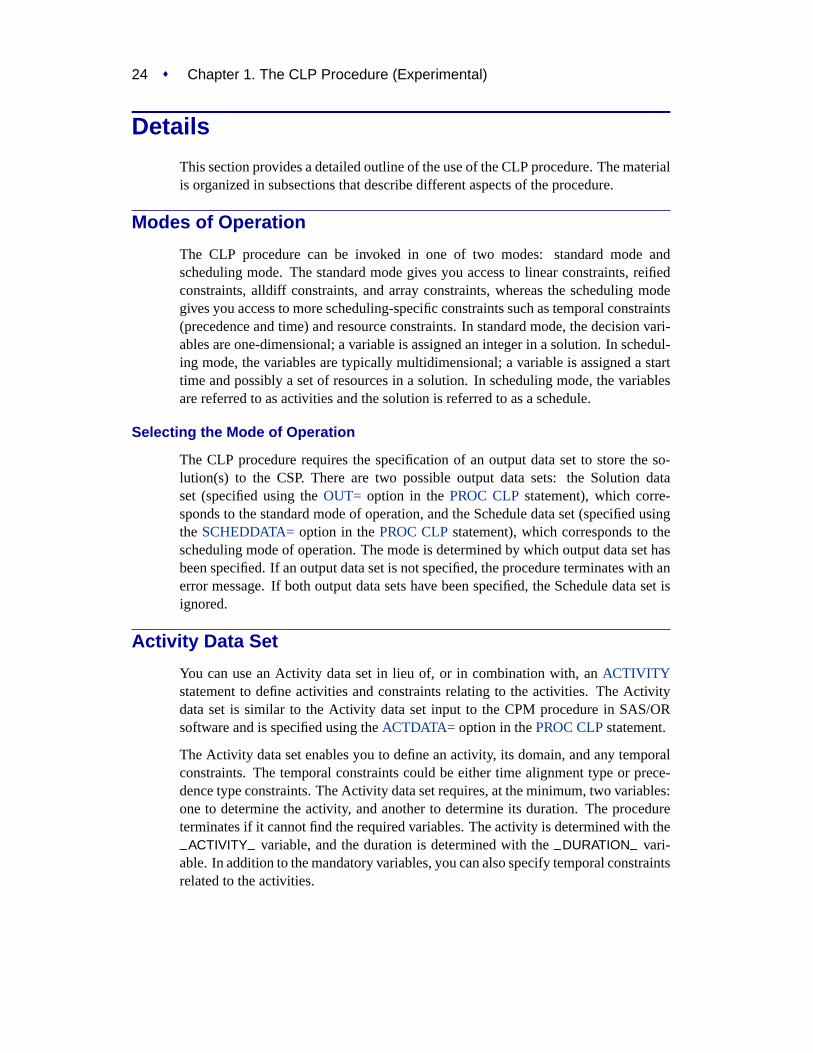
Details

This section provides a detailed outline of the use of the CLP procedure. The materialis organized in subsections that describe different aspects of the procedure.

Modes of Operation

The CLP procedure can be invoked in one of two modes: standard mode andscheduling mode. The standard mode gives you access to linear constraints, reifiedconstraints, alldiff constraints, and array constraints, whereas the scheduling modegives you access to more scheduling-specific constraints such as temporal constraints(precedence and time) and resource constraints. In standard mode, the decision vari-ables are one-dimensional; a variable is assigned an integer in a solution. In schedul-ing mode, the variables are typically multidimensional; a variable is assigned a starttime and possibly a set of resources in a solution. In scheduling mode, the variablesare referred to as activities and the solution is referred to as a schedule.

Selecting the Mode of Operation

The CLP procedure requires the specification of an output data set to store the so-lution(s) to the CSP. There are two possible output data sets: the Solution dataset (specified using theOUT= option in thePROC CLPstatement), which corre-sponds to the standard mode of operation, and the Schedule data set (specified usingthe SCHEDDATA= option in thePROC CLPstatement), which corresponds to thescheduling mode of operation. The mode is determined by which output data set hasbeen specified. If an output data set is not specified, the procedure terminates with anerror message. If both output data sets have been specified, the Schedule data set isignored.

Activity Data Set

You can use an Activity data set in lieu of, or in combination with, anACTIVITYstatement to define activities and constraints relating to the activities. The Activitydata set is similar to the Activity data set input to the CPM procedure in SAS/ORsoftware and is specified using theACTDATA= option in thePROC CLPstatement.

The Activity data set enables you to define an activity, its domain, and any temporalconstraints. The temporal constraints could be either time alignment type or prece-dence type constraints. The Activity data set requires, at the minimum, two variables:one to determine the activity, and another to determine its duration. The procedureterminates if it cannot find the required variables. The activity is determined with the

–ACTIVITY– variable, and the duration is determined with the–DURATION– vari-able. In addition to the mandatory variables, you can also specify temporal constraintsrelated to the activities.

Activity Data Set � 25

Time Alignment Constraints

The –ALIGNDATE– and–ALIGNTYPE– variables enable you to define time align-ment type constraints. The–ALIGNTYPE– variable defines the type of the alignmentconstraint for the activity named in the–ACTIVITY– variable with respect to the

–ALIGNDATE– variable. If the–ALIGNDATE– variable is not present in the Activitydata set, the–ALIGNTYPE– variable is ignored. If the–ALIGNDATE– is present butthe –ALIGNTYPE– variable is missing, the alignment type is assumed to be SGE.The–ALIGNTYPE– variable can take the values shown inTable 1.10:

Table 1.10. Valid Values for the –ALIGNTYPE– Variable

Value Type of AlignmentSEQ Start equal toSGE Start greater than or equal toSLE Start less than or equal toFEQ Finish equal toFGE Finish greater than or equal toFLE Finish less than or equal to

Precedence Constraints

The –SUCCESSOR– variable enables you to define precedence type relationshipsbetween activities using AON (Activity-On-Node) format. The–SUCCESSOR–variable must have the same type as that of the–ACTIVITY– variable. The–LAG–variable defines the lag type of the relationship. By default, all precedence relation-ships are considered to beFinish-to-Start(FS). An FS type of precedence relationshipis also referred to as astandardprecedence constraint. All other types of prece-dence relationships are considered to be nonstandard precedence constraints. The

–LAGDUR– variable specifies the lag duration. By default, the lag duration is zero.

For each (activity, successor) pair, you can define a lag type and a lag duration.Consider the pair of activities (A, B) with a lag duration given bylagdur. The in-terpretation of each of the different lag types is given inTable 1.11.

Table 1.11. Valid Values for the –LAG– Variable

Lag Type InterpretationFS Finish A + lagdur≤ Start BSS Start A + lagdur≤ Start BFF Finish A + lagdur≤ Finish BSF Start A + lagdur≤ Finish BFSE Finish A + lagdur = Start BSSE Start A + lagdur = Start BFFE Finish A + lagdur = Finish BSFE Start A + lagdur = Finish B


The first four lag types (FS, SS, FF, and SF) are also referred to asFinish-to-Start,Start-to-Start, Finish-to-Finish, andStart-to-Finish, respectively. The next four types(FSE, SSE, FFE, and SFE) are stricter versions of FS, SS, FF, and SF, respectively.The first four types impose a lower bound on the start/finish times of B, while the lastfour types force the start/finish times to be set equal to the lower bound of the domain.This enables you to force an activity to begin when its predecessor is finished. Itis relatively easy to generate infeasible scenarios with the stricter versions, so youshould only use the stricter versions if the weaker versions are not adequate for yourproblem.

Resource Constraints

The Activity data set cannot be used to define resource requirement type constraints.To define resource requirement type constraints, you must specifyRESOURCEandREQUIRESstatements.

Variables in the ACTDATA= data set

Table 1.12lists all the variables associated with the Activity data set and their inter-pretations by the CLP procedure. The table also lists for each variable its type (C forcharacter, N for numeric), the possible values it can assume, and its default value.

Table 1.12. Activity Data Set VariablesName Type Description Allowed Values Default

–ACTIVITY– C/N activity name

–DURATION– N duration 0

–SUCCESSOR– C/N successor name same type as

–ACTIVITY––ALIGNDATE– N alignment date 0

–ALIGNTYPE– C alignment type SGE, SLE, SEQ,FGE, FLE, FEQ

SGE

–LAG– C lag type FS, SS, FF, SF,FSE, SSE, FFE, SFE

FS

–LAGDUR– N lag duration 0

Schedule Data Set

In order to solve a scheduling type CSP, you need to specify a Schedule data setusing theSCHEDDATA=option in thePROC CLPstatement. The Schedule data setcontains all the solutions that have been determined by the CLP procedure.

The Schedule data set always contains the following five variables:SOLUTION,ACTIVITY, DUR, START, and FINISH. If any resources have been specified, thenthere is also a variable corresponding to each resource with the name of the variablebeing the name of the resource. TheSOLUTION variable gives the solution numberthat each observation corresponds to. TheACTIVITY variable identifies the activity,theDUR variable gives the duration of the activity, and theSTART andFINISH vari-ables give the scheduled start and finish times for the activity. If there are resourcespresent, the corresponding resource variable indicates whether or not it is being uti-lized for the activity.

Constraint Data Set � 27

For every solution found and for each activity, the Schedule data set contains anobservation that lists the assignment information for that activity.

If an Activity data set has been specified, then the formats and labels for theACTIVITYandDUR variables carry over to the Schedule data set.

Constraint Data Set

The Constraint data set defines linear constraints, variable types, and bounds on vari-able domains. You can use a Constraint data set in lieu of, or in combination with, aLINCON and/or aVAR statement in order to define linear constraints, variable types,and variable bounds. The Constraint data set is similar to the problem data set inputto the LP procedure in SAS/OR software and is specified using theDATA= option inthePROC CLPstatement.

The Constraint data set must be in dense input format. In the dense input format, amodel’s columns appear as variables in the input data set and the data set must con-tain the–TYPE– variable, the–RHS– variable, and at least one numeric variable. Inthe absence of the above requirement, the CLP procedure terminates. The–TYPE–variable is a character variable which tells the CLP procedure how to interpret eachobservation. The CLP procedure recognizes the following keywords as valid val-ues for the–TYPE– variable: EQ, LE, GE, NE, LT, GT, LOWERBD, UPPERBD,BINARY, and FIXED. An optional character variable,–ID– , can be used to nameeach row in the Constraint data set.

Linear Constraints

For the–TYPE– values EQ, LE, GE, NE, LT, GT, the corresponding observationis interpreted as a linear constraint. The–RHS– variable is a numeric variable thatcontains the right-hand-side coefficient of the linear constraint. Any numeric variableother than–RHS– is interpreted as a structural variable for the linear constraint.

Domain Bounds

The values LOWERBD and UPPERBD specify additional lower bounds and upperbounds on the variable domains. In an observation where the–TYPE– variable isequal to LOWERBD, a nonmissing value for a decision variable is considered a lowerbound for that variable. Similarly, in an observation where the–TYPE– variable isequal to UPPERBD, a nonmissing values for a decision variable is considered anupper bound for that variable. In both the above instances, it is important to note thatany specified lower or upper bounds on a variable must be consistent with the existingdomain of the variable, or the problem is deemed infeasible.

Variable Types

The keywords BINARY and FIXED are interpreted as specifying numeric types. Ifthe value of–TYPE– is BINARY for an observation, then any decision variable witha nonmissing entry for the observation is interpreted as being a binary variable withdomain {0,1}. If the value of–TYPE– is FIXED for an observation, then any decisionvariable with a nonmissing entry for the observation is interpreted as being assignedto that nonmissing value. In other words, if the value of the variableX is c in an


observation for which–TYPE– is FIXED, then the domain ofX is considered to bethe singleton{c}. It is important to note that the valuec should belong to the domainof X, or the problem is deemed infeasible.

Any numeric variable other than–RHS– is implicitly considered as appearing in aVAR statement and does not require a separate definition in aVAR statement. In theevent that a numeric variable has previously been defined in aVAR statement, anybounds that are defined in the Constraint data set are considered in addition to boundsthat may have been defined using theVAR statement.

Variables in the DATA= data set

Table 1.13lists all the variables associated with the Constraint data set and theirinterpretations by the CLP procedure. The table also lists for each variable its type (Cfor character, N for numeric), the possible values it can assume, and its default value.

Table 1.13. Constraint Data Set VariablesName Type Description Allowed Values Default

–TYPE– C observation type EQ, LE, GE, NE,LT, GT, LOWERBD,UPPERBD, BINARY,FIXED

–RHS– N right-hand-sidecoefficient

0

–ID– C observation name(optional)

Any numericvariable otherthan–RHS–

N structural variable

Solution Data Set

In order to solve a standard (nonscheduling) type CSP, you need to specify a Solutiondata set using theOUT= option in thePROC CLPstatement. The Solution data setcontains all the solutions that have been determined by the CLP procedure.

The Solution data set contains as many decision variables as have been defined inthe call to PROC CLP. Every observation in the Solution data set corresponds toa solution to the CSP. If a Problem data set has been specified, then any variableformats and variable labels from the Problem data set carry over to the Solution dataset.

References � 29

References

Applegate, D. and Cook, W. (1991), “A Computational Study of the Job ShopScheduling Problem,”ORSA Journal on Computing, 3, 149–156.

Colmerauer, A. (1990), “An Introduction to PROLOG III,”Communications of theACM, 33, 70–90.

Floyd, R. W. (1967), “Nondeterministic Algorithms,”Journal of the ACM, 14,636–644.

Garey, M. R. and Johnson, D. S. (1979),Computers and Intractability: A Guide tothe Theory of NP-Completeness, New York: W. H. Freeman & Co.

Haralick, R. M. and Elliot, G. L. (1980), “Increasing Tree Search Efficiency forConstraint Satisfaction Problems,”Artificial Intelligence, 14, 263–313.

Jaffar, J. and Lassez, J. (1987), “Constraint Logic Programming,”Conference Recordof the 14th Annual ACM Symposium in Principles of Programming Languages,Munich, 111–119.

Kumar, V. (1992), “Algorithms for Constraint-Satisfaction Problems: A Survey,”AIMagazine, 13, 32–44.

Mackworth, A. K. (1977), “Consistency in Networks of Relations,”ArtificialIntelligence, 8, 99–118.

Nemhauser, G. L. and Wolsey, L. A. (1988),Integer and Combinatorial Optimization,New York: John Wiley.

Nuijten, W. (1994), Time and Resource Constrained Scheduling, Ph.D. thesis,Eindhoven Institute of Technology.

Smith, B. M., Brailsford, S. C., Hubbard, P. M., and Williams, H. P. (1996),“The Progressive Party Problem: Integer Linear Programming and ConstraintProgramming Compared,”Constraints, 1, 119–138.

Tsang, E. (1993),Foundations of Constraint Satisfaction, London: Academic Press.

Van Hentenryck, P. (1989),Constraint Satisfaction in Logic Programming,Cambridge, MA: MIT Press.

Van Hentenryck, P., Deville, Y., and Teng, C. (1992), “A Generic Arc-ConsistencyAlgorithm and its Specializations,”Artificial Intelligence, 57, 291–321.

Waltz, D. L. (1975), “Understanding Line Drawings of Scenes with Shadows,” inP. H. Winston, ed., “The Psychology of Computer Vision,” 19–91, New York:McGraw-Hill.

Williams, H. P. and Wilson, J. M. (1998), “Connections Between Integer LinearProgramming and Constraint Logic Programming – An Overview and Introductionto the Cluster of Articles,”INFORMS Journal of Computing, 10, 261–264.

Chapter 1 The CLP Procedure (Experimental)support.sas.com/publishing/pubcat/chaps/59309.pdf ·...

Documents

Transcript of Chapter 1 The CLP Procedure (Experimental)support.sas.com/publishing/pubcat/chaps/59309.pdf ·...