The CLP Procedure - SAS
130
SAS/OR ® 14.1 User’s Guide: Constraint Programming The CLP Procedure
Transcript of The CLP Procedure - SAS

SAS/OR® 14.1 User’s Guide:Constraint ProgrammingThe CLP Procedure

This document is an individual chapter from SAS/OR® 14.1 User’s Guide: Constraint Programming.
The correct bibliographic citation for this manual is as follows: SAS Institute Inc. 2015. SAS/OR® 14.1 User’s Guide: ConstraintProgramming. Cary, NC: SAS Institute Inc.
SAS/OR® 14.1 User’s Guide: Constraint Programming
Copyright © 2015, SAS Institute Inc., Cary, NC, USA
All Rights Reserved. Produced in the United States of America.
For a hard-copy book: No part of this publication may be reproduced, stored in a retrieval system, or transmitted, in any form or byany means, electronic, mechanical, photocopying, or otherwise, without the prior written permission of the publisher, SAS InstituteInc.
For a web download or e-book: Your use of this publication shall be governed by the terms established by the vendor at the timeyou acquire this publication.
The scanning, uploading, and distribution of this book via the Internet or any other means without the permission of the publisher isillegal and punishable by law. Please purchase only authorized electronic editions and do not participate in or encourage electronicpiracy of copyrighted materials. Your support of others’ rights is appreciated.
U.S. Government License Rights; Restricted Rights: The Software and its documentation is commercial computer softwaredeveloped at private expense and is provided with RESTRICTED RIGHTS to the United States Government. Use, duplication, ordisclosure of the Software by the United States Government is subject to the license terms of this Agreement pursuant to, asapplicable, FAR 12.212, DFAR 227.7202-1(a), DFAR 227.7202-3(a), and DFAR 227.7202-4, and, to the extent required under U.S.federal law, the minimum restricted rights as set out in FAR 52.227-19 (DEC 2007). If FAR 52.227-19 is applicable, this provisionserves as notice under clause (c) thereof and no other notice is required to be affixed to the Software or documentation. TheGovernment’s rights in Software and documentation shall be only those set forth in this Agreement.
SAS Institute Inc., SAS Campus Drive, Cary, NC 27513-2414
July 2015
SAS® and all other SAS Institute Inc. product or service names are registered trademarks or trademarks of SAS Institute Inc. in theUSA and other countries. ® indicates USA registration.
Other brand and product names are trademarks of their respective companies.

Chapter 3
The CLP Procedure
ContentsOverview: CLP Procedure . . . . . . . . . . . . . . . . . . . . . . . . . . . . . . . . . . . 12
The Constraint Satisfaction Problem . . . . . . . . . . . . . . . . . . . . . . . . . . . 12Techniques for Solving CSPs . . . . . . . . . . . . . . . . . . . . . . . . . . . . . . 13The CLP Procedure . . . . . . . . . . . . . . . . . . . . . . . . . . . . . . . . . . . 15
Getting Started: CLP Procedure . . . . . . . . . . . . . . . . . . . . . . . . . . . . . . . . 16Send More Money . . . . . . . . . . . . . . . . . . . . . . . . . . . . . . . . . . . . 16Eight Queens . . . . . . . . . . . . . . . . . . . . . . . . . . . . . . . . . . . . . . . 17
Syntax: CLP Procedure . . . . . . . . . . . . . . . . . . . . . . . . . . . . . . . . . . . . . 19Functional Summary . . . . . . . . . . . . . . . . . . . . . . . . . . . . . . . . . . . 20PROC CLP Statement . . . . . . . . . . . . . . . . . . . . . . . . . . . . . . . . . . 22ACTIVITY Statement . . . . . . . . . . . . . . . . . . . . . . . . . . . . . . . . . . 26ALLDIFF Statement . . . . . . . . . . . . . . . . . . . . . . . . . . . . . . . . . . . 27ARRAY Statement . . . . . . . . . . . . . . . . . . . . . . . . . . . . . . . . . . . . 27ELEMENT Statement . . . . . . . . . . . . . . . . . . . . . . . . . . . . . . . . . . 27FOREACH Statement . . . . . . . . . . . . . . . . . . . . . . . . . . . . . . . . . . 28GCC Statement . . . . . . . . . . . . . . . . . . . . . . . . . . . . . . . . . . . . . . 29LEXICO Statement . . . . . . . . . . . . . . . . . . . . . . . . . . . . . . . . . . . 30LINCON Statement . . . . . . . . . . . . . . . . . . . . . . . . . . . . . . . . . . . 31OBJ Statement . . . . . . . . . . . . . . . . . . . . . . . . . . . . . . . . . . . . . . 32PACK Statement . . . . . . . . . . . . . . . . . . . . . . . . . . . . . . . . . . . . . 32REIFY Statement . . . . . . . . . . . . . . . . . . . . . . . . . . . . . . . . . . . . 33REQUIRES Statement . . . . . . . . . . . . . . . . . . . . . . . . . . . . . . . . . . 34RESOURCE Statement . . . . . . . . . . . . . . . . . . . . . . . . . . . . . . . . . 36SCHEDULE Statement . . . . . . . . . . . . . . . . . . . . . . . . . . . . . . . . . 36VARIABLE Statement . . . . . . . . . . . . . . . . . . . . . . . . . . . . . . . . . . 41
Details: CLP Procedure . . . . . . . . . . . . . . . . . . . . . . . . . . . . . . . . . . . . . 41Modes of Operation . . . . . . . . . . . . . . . . . . . . . . . . . . . . . . . . . . . 41Constraint Data Set . . . . . . . . . . . . . . . . . . . . . . . . . . . . . . . . . . . . 42Solution Data Set . . . . . . . . . . . . . . . . . . . . . . . . . . . . . . . . . . . . . 44Activity Data Set . . . . . . . . . . . . . . . . . . . . . . . . . . . . . . . . . . . . . 45Resource Data Set . . . . . . . . . . . . . . . . . . . . . . . . . . . . . . . . . . . . 47Schedule Data Set . . . . . . . . . . . . . . . . . . . . . . . . . . . . . . . . . . . . 48SCHEDRES= Data Set . . . . . . . . . . . . . . . . . . . . . . . . . . . . . . . . . 50SCHEDTIME= Data Set . . . . . . . . . . . . . . . . . . . . . . . . . . . . . . . . . 50Edge Finding . . . . . . . . . . . . . . . . . . . . . . . . . . . . . . . . . . . . . . . 50Macro Variable _ORCLP_ . . . . . . . . . . . . . . . . . . . . . . . . . . . . . . . . 50

12 F Chapter 3: The CLP Procedure
Macro Variable _ORCLPEAS_ . . . . . . . . . . . . . . . . . . . . . . . . . . . . . 52Macro Variable _ORCLPEVS_ . . . . . . . . . . . . . . . . . . . . . . . . . . . . . 52
Examples: CLP Procedure . . . . . . . . . . . . . . . . . . . . . . . . . . . . . . . . . . . 53Example 3.1: Logic-Based Puzzles . . . . . . . . . . . . . . . . . . . . . . . . . . . 54Example 3.2: Alphabet Blocks Problem . . . . . . . . . . . . . . . . . . . . . . . . . 64Example 3.3: Work-Shift Scheduling Problem . . . . . . . . . . . . . . . . . . . . . 66Example 3.4: A Nonlinear Optimization Problem . . . . . . . . . . . . . . . . . . . . 70Example 3.5: Car Painting Problem . . . . . . . . . . . . . . . . . . . . . . . . . . . 71Example 3.6: Scene Allocation Problem . . . . . . . . . . . . . . . . . . . . . . . . . 73Example 3.7: Car Sequencing Problem . . . . . . . . . . . . . . . . . . . . . . . . . 78Example 3.8: Round-Robin Problem . . . . . . . . . . . . . . . . . . . . . . . . . . 82Example 3.9: Resource-Constrained Scheduling with Nonstandard Temporal Constraints 85Example 3.10: Scheduling with Alternate Resources . . . . . . . . . . . . . . . . . . 94Example 3.11: 10×10 Job Shop Scheduling Problem . . . . . . . . . . . . . . . . . . 102Example 3.12: Scheduling a Major Basketball Conference . . . . . . . . . . . . . . . 105Example 3.13: Balanced Incomplete Block Design . . . . . . . . . . . . . . . . . . . 115Example 3.14: Progressive Party Problem . . . . . . . . . . . . . . . . . . . . . . . . 121Statement and Option Cross-Reference Table . . . . . . . . . . . . . . . . . . . . . . 128
References . . . . . . . . . . . . . . . . . . . . . . . . . . . . . . . . . . . . . . . . . . . 129
Overview: CLP ProcedureThe CLP procedure is a finite-domain constraint programming solver for constraint satisfaction problems(CSPs) with linear, logical, global, and scheduling constraints. In addition to having an expressive syntaxfor representing CSPs, the CLP procedure features powerful built-in consistency routines and constraintpropagation algorithms, a choice of nondeterministic search strategies, and controls for guiding the searchmechanism that enable you to solve a diverse array of combinatorial problems.
You can also solve standard constraint satisfaction problems via the constraint programming solver in PROCOPTMODEL. For more information, see the constraint programming solver chapter in SAS/OR User’s Guide:Mathematical Programming.
The Constraint Satisfaction ProblemMany important problems in areas such as artificial intelligence (AI) and operations research (OR) canbe formulated as constraint satisfaction problems. A CSP is defined by a finite set of variables that takevalues from finite domains and by a finite set of constraints that restrict the values that the variables cansimultaneously take.
More formally, a CSP can be defined as a triple hX;D;C i:
� X D fx1; : : : ; xng is a finite set of variables.

Techniques for Solving CSPs F 13
� D D fD1; : : : ;Dng is a finite set of domains, where Di is a finite set of possible values that thevariable xi can take. Di is known as the domain of variable xi .
� C D fc1; : : : ; cmg is a finite set of constraints that restrict the values that the variables can simultane-ously take.
The domains need not represent consecutive integers. For example, the domain of a variable could be the setof all even numbers in the interval [0, 100]. A domain does not even need to be totally numeric. In fact, in ascheduling problem with resources, the values are typically multidimensional. For example, an activity canbe considered as a variable, and each element of the domain would be an n-tuple that represents a start timefor the activity and one or more resources that must be assigned to the activity that corresponds to the starttime.
A solution to a CSP is an assignment of values to the variables in order to satisfy all the constraints. Theproblem amounts to finding one or more solutions, or possibly determining that a solution does not exist.
The CLP procedure can be used to find one or more (and in some instances, all) solutions to a CSP withlinear, logical, global, and scheduling constraints. The numeric components of all variable domains areassumed to be integers.
Techniques for Solving CSPsSeveral techniques for solving CSPs are available. Kumar (1992) and Tsang (1993) present a good overviewof these techniques. It should be noted that the satisfiability problem (SAT) (Garey and Johnson 1979) canbe regarded as a CSP. Consequently, most problems in this class are non-deterministic polynomial-timecomplete (NP-complete) problems, and a backtracking search mechanism is an important technique forsolving them (Floyd 1967).
One of the most popular tree search mechanisms is chronological backtracking. However, a chronologicalbacktracking approach is not very efficient due to the late detection of conflicts; that is, it is oriented towardrecovering from failures rather than avoiding them to begin with. The search space is reduced only afterdetection of a failure, and the performance of this technique is drastically reduced with increasing problemsize. Another drawback of using chronological backtracking is encountering repeated failures due to thesame reason, sometimes referred to as “thrashing.” The presence of late detection and “thrashing” has ledresearchers to develop consistency techniques that can achieve superior pruning of the search tree. Thisstrategy employs an active use, rather than a passive use, of constraints.
Constraint Propagation
A more efficient technique than backtracking is that of constraint propagation, which uses consistencytechniques to effectively prune the domains of variables. Consistency techniques are based on the idea of apriori pruning, which uses the constraint to reduce the domains of the variables. Consistency techniques arealso known as relaxation algorithms (Tsang 1993), and the process is also referred to as problem reduction,domain filtering, or pruning.
One of the earliest applications of consistency techniques was in the AI field in solving the scene labelingproblem, which required recognizing objects in three-dimensional space by interpreting two-dimensional linedrawings of the object. The Waltz filtering algorithm (Waltz 1975) analyzes line drawings by systematicallylabeling the edges and junctions while maintaining consistency between the labels.

14 F Chapter 3: The CLP Procedure
An effective consistency technique for handling resource capacity constraints is edge finding (Applegate andCook 1991). Edge-finding techniques reason about the processing order of a set of activities that requirea given resource or set of resources. Some of the earliest work related to edge finding can be attributed toCarlier and Pinson (1989), who successfully solved MT10, a well-known 10×10 job shop problem that hadremain unsolved for over 20 years (Muth and Thompson 1963).
Constraint propagation is characterized by the extent of propagation (also referred to as the level of con-sistency) and the domain pruning scheme that is followed: domain propagation or interval propagation. Inpractice, interval propagation is preferred over domain propagation because of its lower computational costs.This mechanism is discussed in detail in Van Hentenryck (1989). However, constraint propagation is not acomplete solution technique and needs to be complemented by a search technique in order to ensure success(Kumar 1992).
Finite-Domain Constraint Programming
Finite-domain constraint programming is an effective and complete solution technique that embeds incompleteconstraint propagation techniques into a nondeterministic backtracking search mechanism, implementedas follows. Whenever a node is visited, constraint propagation is carried out to attain a desired level ofconsistency. If the domain of each variable reduces to a singleton set, the node represents a solution to theCSP. If the domain of a variable becomes empty, the node is pruned. Otherwise a variable is selected, itsdomain is distributed, and a new set of CSPs is generated, each of which is a child node of the current node.Several factors play a role in determining the outcome of this mechanism, such as the extent of propagation(or level of consistency enforced), the variable selection strategy, and the variable assignment or domaindistribution strategy.
For example, the lack of any propagation reduces this technique to a simple generate-and-test, whereasperforming consistency on variables already selected reduces this to chronological backtracking, one ofthe systematic search techniques. These are also known as look-back schemas, because they share thedisadvantage of late conflict detection. Look-ahead schemas, on the other hand, work to prevent futureconflicts. Some popular examples of look-ahead strategies, in increasing degree of consistency level, areforward checking (FC), partial look ahead (PLA), and full look ahead (LA) (Kumar 1992). Forward checkingenforces consistency between the current variable and future variables; PLA and LA extend this even furtherto pairs of not yet instantiated variables.
Two important consequences of this technique are that inconsistencies are discovered early and that thecurrent set of alternatives that are coherent with the existing partial solution is dynamically maintained. Theseconsequences are powerful enough to prune large parts of the search tree, thereby reducing the “combinatorialexplosion” of the search process. However, although constraint propagation at each node results in fewernodes in the search tree, the processing at each node is more expensive. The ideal scenario is to strike abalance between the extent of propagation and the subsequent computation cost.
Variable selection is another strategy that can affect the solution process. The order in which variables arechosen for instantiation can have a substantial impact on the complexity of the backtrack search. Severalheuristics have been developed and analyzed for selecting variable ordering. One of the more common onesis a dynamic heuristic based on the fail first principle (Haralick and Elliott 1980), which selects the variablewhose domain has minimal size. Subsequent analysis of this heuristic by several researchers has validatedthis technique as providing substantial improvement for a significant class of problems. Another populartechnique is to instantiate the most constrained variable first. Both these strategies are based on the principleof selecting the variable most likely to fail and to detect such failures as early as possible.

The CLP Procedure F 15
The domain distribution strategy for a selected variable is yet another area that can influence the performanceof a backtracking search. However, good value-ordering heuristics are expected to be very problem-specific(Kumar 1992).
The CLP ProcedureThe CLP procedure is a finite-domain constraint programming solver for CSPs. In the context of the CLPprocedure, CSPs can be classified into the following two types, which are determined by specification of therelevant output data set:
� A standard CSP is characterized by integer variables, linear constraints, array-type constraints, globalconstraints, and reify constraints. In other words, X is a finite set of integer variables, and C can containlinear, array, global, or logical constraints. Specifying the OUT= option in the PROC CLP statementindicates to the CLP procedure that the CSP is a standard-type CSP. As such, the procedure expectsonly VARIABLE, ALLDIFF, ELEMENT, GCC, LEXICO, LINCON, PACK, REIFY, ARRAY, andFOREACH statements. You can also specify a Constraint data set by using the CONDATA= option inthe PROC CLP statement instead of, or in combination with, VARIABLE and LINCON statements.
� A scheduling CSP is characterized by activities, temporal constraints, and resource requirement con-straints. In other words, X is a finite set of activities, and C is a set of temporal constraints and resourcerequirement constraints. Specifying one of the SCHEDULE=, SCHEDRES=, or SCHEDTIME=options in the PROC CLP statement indicates to the CLP procedure that the CSP is a scheduling-typeCSP. As such, the procedure expects only ACTIVITY, RESOURCE, REQUIRES, and SCHEDULEstatements. You can also specify an Activity data set by using the ACTDATA= option in the PROCCLP statement instead of, or in combination with, the ACTIVITY, RESOURCE, and REQUIRESstatements. You can define activities by using the Activity data set or the ACTIVITY statement. Prece-dence relationships between activities must be defined using the ACTDATA= data set. You can defineresource requirements of activities by using the Activity data set or the RESOURCE and REQUIRESstatements.
The output data sets contain any solutions determined by the CLP procedure. For more information about theformat and layout of the output data sets, see the sections “Solution Data Set” on page 44 and “ScheduleData Set” on page 48.
Consistency Techniques
The CLP procedure features a full look-ahead algorithm for standard CSPs that follows a strategy ofmaintaining a version of generalized arc consistency that is based on the AC-3 consistency routine (Mackworth1977). This strategy maintains consistency between the selected variables and the unassigned variables andalso maintains consistency between unassigned variables. For the scheduling CSPs, the CLP procedure usesa forward-checking algorithm, an arc-consistency routine for maintaining consistency between unassignedactivities, and energetic-based reasoning methods for resource-constrained scheduling that feature the edge-finder algorithm (Applegate and Cook 1991). You can elect to turn off some of these consistency techniquesin the interest of performance.

16 F Chapter 3: The CLP Procedure
Selection Strategy
A search algorithm for CSPs searches systematically through the possible assignments of values to variables.The order in which a variable is selected can be based on a static ordering, which is determined before thesearch begins, or on a dynamic ordering, in which the choice of the next variable depends on the current stateof the search. The VARSELECT= option in the PROC CLP statement defines the variable selection strategyfor a standard CSP. The default strategy is the dynamic MINR strategy, which selects the variable withthe smallest range. The ACTSELECT= option in the SCHEDULE statement defines the activity selectionstrategy for a scheduling CSP. The default strategy is the RAND strategy, which selects an activity at randomfrom the set of activities that begin prior to the earliest early finish time. This strategy was proposed byNuijten (1994).
Assignment Strategy
After a variable or an activity has been selected, the assignment strategy dictates the value that is assignedto it. For variables, the assignment strategy is specified with the VARASSIGN= option in the PROC CLPstatement. The default assignment strategy selects the minimum value from the domain of the selectedvariable. For activities, the assignment strategy is specified with the ACTASSIGN= option in the SCHEDULEstatement. The default strategy of RAND assigns the time to the earliest start time, and the resources arechosen randomly from the set of resource assignments that support the selected start time.
Getting Started: CLP ProcedureThe following examples illustrate the use of the CLP procedure in the formulation and solution of twowell-known logical puzzles in the constraint programming community.
Send More MoneyThe Send More Money problem consists of finding unique digits for the letters D, E, M, N, O, R, S, and Ysuch that S and M are different from zero (no leading zeros) and the following equation is satisfied:
S E N D
+ M O R E
M O N E Y
You can use the CLP procedure to formulate this problem as a CSP by representing each of the letters inthe expression with an integer variable. The domain of each variable is the set of digits 0 through 9. TheVARIABLE statement identifies the variables in the problem. The DOM= option defines the default domainfor all the variables to be [0,9]. The OUT= option identifies the CSP as a standard type. The LINCONstatement defines the linear constraint SEND + MORE = MONEY, and the restrictions that S and M cannot

Eight Queens F 17
take the value zero. (Alternatively, you can simply specify the domain for S and M as [1,9] in the VARIABLEstatement.) Finally, the ALLDIFF statement is specified to enforce the condition that the assignment of digitsshould be unique. The complete representation, using the CLP procedure, is as follows:
proc clp dom=[0,9] /* Define the default domain */out=out; /* Name the output data set */
var S E N D M O R E M O N E Y; /* Declare the variables */lincon /* Linear constraints */
/* SEND + MORE = MONEY */1000*S + 100*E + 10*N + D + 1000*M + 100*O + 10*R + E=10000*M + 1000*O + 100*N + 10*E + Y,S<>0, /* No leading zeros */M<>0;
alldiff(); /* All variables have pairwise distinct values*/run;
The solution data set produced by the CLP procedure is shown in Figure 3.1.
Figure 3.1 Solution to SEND + MORE = MONEY
S E N D M O R Y
9 5 6 7 1 0 8 2
The unique solution to the problem determined by the CLP procedure is as follows:
9 5 6 7
+ 1 0 8 5
1 0 6 5 2
Eight QueensThe Eight Queens problem is a special instance of the N-Queens problem, where the objective is to positionN queens on an N×N chessboard such that no two queens attack each other. The CLP procedure provides anexpressive constraint for variable arrays that can be used for solving this problem very efficiently.
You can model this problem by using a variable array A of dimension N, where AŒi� is the row number of thequeen in column i. Since no two queens can be in the same row, it follows that all the AŒi�’s must be pairwisedistinct.
In order to ensure that no two queens can be on the same diagonal, the following should be true for all i and j:
AŒj � � AŒi� <> j � i
and
AŒj � � AŒi� <> i � j

18 F Chapter 3: The CLP Procedure
In other words,
AŒi� � i <> AŒj � � j
and
AŒi�C i <> AŒj �C j
Hence, the .AŒi �C i/’s are pairwise distinct, and the .AŒi � � i/’s are pairwise distinct.
These two conditions, in addition to the one requiring that the AŒi�’s be pairwise distinct, can be formulatedusing the FOREACH statement.
One possible such CLP formulation is presented as follows:
proc clp out=outvarselect=fifo; /* Variable Selection Strategy */
array A[8] (A1-A8); /* Define the array A */var (A1-A8)=[1,8]; /* Define each of the variables in the array */
/* Initialize domains *//* A[i] is the row number of the queen in column i*/foreach(A, DIFF, 0); /* A[i] 's are pairwise distinct */foreach(A, DIFF, -1); /* A[i] - i 's are pairwise distinct */foreach(A, DIFF, 1); /* A[i] + i 's are pairwise distinct */
run;
The ARRAY statement is required when you are using a FOREACH statement, and it defines the arrayA in terms of the eight variables A1–A8. The domain of each of these variables is explicitly specifiedin the VARIABLE statement to be the digits 1 through 8 since they represent the row number on an 8×8board. FOREACH(A, DIFF, 0) represents the constraint that the AŒi�’s are different. FOREACH(A, DIFF,–1) represents the constraint that the .AŒi � � i/’s are different, and FOREACH(A, DIFF, 1) represents theconstraint that the .AŒi � C i/’s are different. The VARSELECT= option specifies the variable selectionstrategy to be first-in-first-out, the order in which the variables are encountered by the CLP procedure.
The following statements display the solution data set shown in Figure 3.2:
proc print data=out noobs label;label A1=a A2=b A3=c A4=d
A5=e A6=f A7=g A8=h;run;
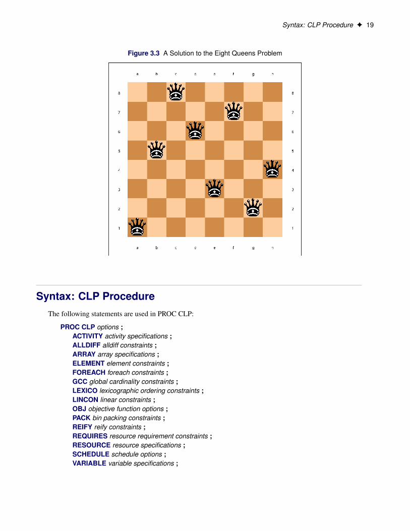
Figure 3.2 A Solution to the Eight Queens Problem
a b c d e f g h
1 5 8 6 3 7 2 4
The corresponding solution to the Eight Queens problem is displayed in Figure 3.3.
Syntax: CLP Procedure F 19
Figure 3.3 A Solution to the Eight Queens Problem
Syntax: CLP ProcedureThe following statements are used in PROC CLP:
PROC CLP options ;ACTIVITY activity specifications ;ALLDIFF alldiff constraints ;ARRAY array specifications ;ELEMENT element constraints ;FOREACH foreach constraints ;GCC global cardinality constraints ;LEXICO lexicographic ordering constraints ;LINCON linear constraints ;OBJ objective function options ;PACK bin packing constraints ;REIFY reify constraints ;REQUIRES resource requirement constraints ;RESOURCE resource specifications ;SCHEDULE schedule options ;VARIABLE variable specifications ;

20 F Chapter 3: The CLP Procedure
Functional SummaryThe statements and options available in PROC CLP are summarized by purpose in Table 3.1.
Table 3.1 Functional Summary
Description Statement Option
Assignment Strategy OptionsSpecifies the variable assignment strategy PROC CLP VARASSIGN=Specifies the activity assignment strategy SCHEDULE ACTASSIGN=
Data Set OptionsSpecifies the activity input data set PROC CLP ACTDATA=Specifies the constraint input data set PROC CLP CONDATA=Specifies the solution output data set PROC CLP OUT=Specifies the resource input data set PROC CLP RESDATA=Specifies the resource assignment data set PROC CLP SCHEDRES=Specifies the time assignment data set PROC CLP SCHEDTIME=Specifies the schedule output data set PROC CLP SCHEDULE=
Domain OptionsSpecifies the global domain of all variables PROC CLP DOMAIN=Specifies the domain for selected variables VARIABLE
General OptionsSpecifies the upper bound on time (seconds) PROC CLP MAXTIME=Suppresses preprocessing PROC CLP NOPREPROCESSPermits preprocessing PROC CLP PREPROCESSSpecifies the units of MAXTIME PROC CLP TIMETYPE=Implicitly defines Constraint data set variables PROC CLP USECONDATAVARS=
Objective Function OptionsSpecifies the lower bound for the objective OBJ LB=Specifies the tolerance for the search OBJ TOL=Specifies the upper bound for the objective OBJ UB=
Output Control OptionsFinds all possible solutions PROC CLP FINDALLSOLNSSpecifies the number of solution attempts PROC CLP MAXSOLNS=Indicates progress in log PROC CLP SHOWPROGRESS
Scheduling CSP-Related StatementsDefines activity specifications ACTIVITYDefines resource requirement specifications REQUIRESDefines resource specifications RESOURCEDefines scheduling parameters SCHEDULE

Functional Summary F 21
Table 3.1 continued
Description Statement Option
Scheduling: Resource ConstraintsSpecifies the edge-finder consistency routines SCHEDULE EDGEFINDER=Specifies the not-first edge-finder extension SCHEDULE NOTFIRST=Specifies the not-last edge-finder extension SCHEDULE NOTLAST=
Scheduling: Temporal ConstraintsSpecifies the activity duration ACTIVITY (DUR=)Specifies the activity finish lower bound ACTIVITY (FGE=)Specifies the activity finish upper bound ACTIVITY (FLE=)Specifies the activity start lower bound ACTIVITY (SGE=)Specifies the activity start upper bound ACTIVITY (SLE=)Specifies the schedule duration SCHEDULE DURATION=Specifies the schedule finish SCHEDULE FINISH=Specifies the schedule start SCHEDULE START=
Scheduling: Search Control OptionsSpecifies the dead-end multiplier PROC CLP DM=Specifies the number of allowable dead ends per restart PROC CLP DPR=Specifies the number of search restarts PROC CLP RESTARTS=
Selection Strategy OptionsSpecifies the variable selection strategy PROC CLP VARSELECT=Specifies the activity selection strategy SCHEDULE ACTSELECT=Specifies variable selection strategies for evaluation PROC CLP EVALVARSEL=Specifies activity selection strategies for evaluation SCHEDULE EVALACTSEL=Enables time limit updating for strategy evaluation PROC CLP DECRMAXTIME
Standard CSP StatementsSpecifies the all-different constraints ALLDIFFSpecifies the array specifications ARRAYSpecifies the element constraints ELEMENTSpecifies the for-each constraints FOREACHSpecifies the global cardinality constraints GCCSpecifies the lexicographic ordering constraints LEXICOSpecifies the linear constraints LINCONSpecifies the bin packing constraints PACKSpecifies the reified constraints REIFYDefines the variable specifications VARIABLE

22 F Chapter 3: The CLP Procedure
PROC CLP StatementPROC CLP options ;
The PROC CLP statement invokes the CLP procedure. You can specify options to control a variety of searchparameters that include selection strategies, assignment strategies, backtracking strategies, maximum runningtime, and number of solution attempts. You can specify the following options:
ACTDATA=SAS-data-set
ACTIVITY=SAS-data-setidentifies the input SAS data set that defines the activities and temporal constraints. The temporalconstraints consist of time-alignment-type constraints and precedence-type constraints. The formatof the ACTDATA= data set is similar to that of the Activity data set used by the CPM procedure inSAS/OR software. You can also specify the activities and time alignment constraints directly by usingthe ACTIVITY statement without the need for a data set. The CLP procedure enables you to defineactivities by using a combination of the two specifications.
CONDATA=SAS-data-setidentifies the input SAS data set that defines the constraints, variable types, and variable bounds. TheCONDATA data set provides support for linear constraints only.
You can also specify the linear constraints in-line by using the LINCON statement. The CLP procedureenables you to define constraints by using a combination of the two specifications. When definingconstraints, you must define the variables by using a VARIABLE statement or implicitly define themby specifying the USECONDATAVARS= option when using the CONDATA= data set. You can definevariable bounds by using the VARIABLE statement, and any such definitions override those defined inthe CONDATA= data set.
DECRMAXTIMEdynamically decreases the maximum solution time in effect during evaluation of the selection strategy.The DECRMAXTIME option is effective only when the EVALACTSEL= option or the EVAL-VARSEL= option is specified. Initially, the maximum solution time is the value specified by theMAXTIME= option. Whenever a solution is found with the current activity or variable selectionstrategy, the value of MAXTIME for future attempts is reduced to the current solution time. TheDECRMAXTIME option thus provides a sense of which strategy is the fastest for a given problem.However, you must use caution when comparing the strategies in the macro variable, because theresults pertain to different time limits.
By default, DECRMAXTIME is disabled; each activity or variable selection strategy is given theamount of time specified by the MAXTIME= option.
DM=mspecifies the dead-end multiplier for the scheduling CSP. The dead-end multiplier is used to determinethe number of dead ends that are permitted before triggering a complete restart of the search techniquein a scheduling environment. The number of dead ends is the product of the dead-end multiplier, m,and the number of unassigned activities. The default value is 0.15. This option is valid only with theSCHEDULE= option.

PROC CLP Statement F 23
DOMAIN=[lb, ub]DOM=[lb, ub]
specifies the global domain of all variables to be the closed interval [lb, ub]. You can override theglobal domain for a variable with a VARIABLE statement or the CONDATA= data set. The defaultdomain is [0,1].
DPR=nspecifies an upper bound on the number of dead ends that are permitted before PROC CLP restartsor terminates the search, depending on whether or not a randomized search strategy is used. In thecase of a nonrandomized strategy, n is an upper bound on the number of allowable dead ends beforeterminating. In the case of a randomized strategy, n is an upper bound on the number of allowabledead ends before restarting the search. The DPR= option has priority over the DM= option.
EVALVARSEL<=(keyword(s))>evaluates specified variable selection strategies by attempting to find a solution with each strategy. Youcan specify any combination of valid variable selection strategies in a space-delimited list enclosedin parentheses. If you do not specify a list, all available strategies are evaluated in alphabetical order,except that the default strategy is evaluated first. Descriptions of the available selection strategies areprovided in the discussion of the VARSELECT= option.
When the EVALVARSEL= option is in effect, the MAXTIME= option must also be specified. Bydefault, the value specified for the MAXTIME= option is used as the maximum solution time for eachvariable selection strategy. When the DECRMAXTIME option is specified and a solution has beenfound, the value of the MAXTIME= option is set to the solution time of the last solution.
After the CLP procedure has attempted to find a solution with a particular strategy, it proceeds to thenext strategy in the list. For this reason, the VARSELECT=, ALLSOLNS, and MAXSOLNS= optionsare ignored when the EVALVARSEL= option is in effect. All solutions found during the evaluationprocess are saved in the output data set specified by the OUT= option.
The macro variable _ORCLPEVS_ provides more information that is related to the evaluation of eachvariable selection strategy. The fastest variable selection strategy is indicated in the macro variable_ORCLP_, provided that either at least one solution is found or the problem is found to be infeasible.See “Macro Variable _ORCLP_” on page 50 for more information about the _ORCLP_ macro variable;see “Macro Variable _ORCLPEVS_” on page 52 for more information about the _ORCLPEVS_ macrovariable.
FINDALLSOLNSALLSOLNSFINDALL
attempts to find all possible solutions to the CSP. When a randomized search strategy is used, it ispossible to rediscover the same solution and end up with multiple instances of the same solution. Thisis currently the case when you are solving a scheduling CSP. Therefore, this option is ignored whenyou are solving a scheduling CSP.
MAXSOLNS=nspecifies the number of solution attempts to be generated for the CSP. The default value is 1. It isimportant to note, especially in the context of randomized strategies, that an attempt could result in nosolution, given the current controls on the search mechanism, such as the number of restarts and thenumber of dead ends permitted. As a result, the total number of solutions found might not match theMAXSOLNS= parameter.

24 F Chapter 3: The CLP Procedure
MAXTIME=nspecifies an upper bound on the number of seconds that are allocated for solving the problem. Thetype of time, either CPU time or real time, is determined by the value of the TIMETYPE= option.The default type is CPU time. The time specified by the MAXTIME= option is checked only once atthe end of each iteration. Therefore, the actual running time can be longer than that specified by theMAXTIME= option. The difference depends on how long the last iteration takes. The default value ofMAXTIME= is1. If you do not specify this option, the procedure does not stop based on the amountof time elapsed.
NOPREPROCESSsuppresses any preprocessing that would typically be performed for the problem.
OUT=SAS-data-setidentifies the output data set that contains one or more solutions to a standard CSP, if one exists. Eachobservation in the OUT= data set corresponds to a solution of the CSP. The number of solutions thatare generated can be controlled using the MAXSOLNS= option in the PROC CLP statement.
PREPROCESSpermits any preprocessing that would typically be performed for the problem.
RESDATA=SAS-data-set
RESIN=SAS-data-setidentifies the input data set that defines the resources and their attributes such as capacity and resourcepool membership. This information can be used in lieu of, or in combination with, the RESOURCEstatement.
RESTARTS=nspecifies the number of restarts of the randomized search technique before terminating the procedure.The default value is 3.
SCHEDRES=SAS-data-setidentifies the output data set that contains the solutions to scheduling CSPs. This data set contains theresource assignments of activities.
SCHEDTIME=SAS-data-setidentifies the output data set that contains the solutions to scheduling CSPs. This data set contains thetime assignments of activities.
SCHEDULE=SAS-data-set
SCHEDOUT=SAS-data-setidentifies the output data set that contains the solutions to a scheduling CSP, if any exist. This dataset contains both the time and resource assignment information. There are two types of observationsidentified by the value of the OBSTYPE variable: observation with OBSTYPE= “TIME” corresponds totime assignment, and observation with OBSTYPE= “RESOURCE” corresponds to resource assignment.The maximum number of solutions can be controlled by using the MAXSOLNS= option in the PROCCLP statement.

PROC CLP Statement F 25
SHOWPROGRESSprints a message to the log whenever a solution has been found. When a randomized strategy is used,the number of restarts and dead ends that were required are also printed to the log.
TIMETYPE=CPU j REALspecifies whether CPU time or real time is used for the MAXTIME= option and the macro variables ina PROC CLP call. The default value of this option is CPU.
USECONDATAVARS=0 j 1specifies whether the numeric variables in the CONDATA= data set, with the exception of any reservedvariables, are implicitly defined or not. A value of 1 indicates they are implicitly defined, in whichcase a VARIABLE statement is not necessary to define the variables in the data set. The default valueis 0. Currently, _RHS_ is the only reserved numeric variable.
VARASSIGN=MAX j MINspecifies the value selection strategy. Currently, there are two value selection strategies:
� MAX, which selects the maximum value from the domain of the selected variable
� MIN, which selects the minimum value from the domain of the selected variable
The default value selection strategy is MIN. To assign activities, use the ACTASSIGN= option in theSCHEDULE statement.
VARSELECT=keywordspecifies the variable selection strategy. The strategy could be static, dynamic or conflict-directed.Typically, static strategies exploit information about the initial state of the search, whereas dynamicstrategies exploit information about the current state of the search process. Conflict-directed strategiesare strategies which exploit information from previous states of the search process as well as the currentstate (Boussemart et al. 2004)
Static strategies are as follows:
� FIFO, which uses the first-in-first-out ordering of the variables as encountered by the procedure
� MAXCS, which selects the variable with the maximum number of constraints (degree)
Dynamic strategies are as follows:
� DOMDDEG, which selects the variable with the smallest ratio of domain size by dynamic degree
� DOMDEG, which selects the variable with the smallest ratio of domain size by degree
� MAXC, which selects the variable with the largest number of active constraints (dynamic degree)
� MINR, which selects the variable with the smallest range (that is, the minimum value of upperbound minus lower bound)
� MINRMAXC, which selects the variable with the smallest range, breaking ties by selecting onewith the largest number of active constraints
Conflict-directed strategies are as follows:
� DOMWDEG, which selects the variable with the smallest ratio of domain size by weighteddegree
� WDEG, which selects the variable with the largest weighted degree
26 F Chapter 3: The CLP Procedure
The dynamic strategies embody the “fail first principle” (FFP) of Haralick and Elliott (1980), whichsuggests that “To succeed, try first where you are most likely to fail.” The degree of a variable is thenumber of constraints in which the variable appears. The dynamic degree of a variable is the degree ofthe variable with respect to the current set of active constraints. Boussemart et al. (2004) introducedthe concept of weighted degree, which takes into account dead ends during searches. Weights areassociated with constraints and variables. The weight of a constraint is initially set to 1 and incrementedeach time the constraint is responsible for a dead end. The weight of a variable is equal to the sum ofthe weights of the active constraints that it is associated with. The default variable selection strategy isMINR. To set the strategy for selecting activities, use the ACTSELECT= option in the SCHEDULEstatement.
ACTIVITY StatementACTIVITY specification-1 < . . . specification-n > ;
An ACTIVITY specification can be one of the following types:
activity < = ( < DUR= > duration < altype=aldate . . . >) >
(activity_list) < = ( < DUR= > duration < altype=aldate . . . >) >
where duration is the activity duration and altype is a keyword that specifies an alignment-type constraint onthe activity (or activities) with respect to the value given by aldate.
The ACTIVITY statement defines one or more activities and the attributes of each activity, such as theduration and any temporal constraints of the time-alignment-type. The activity duration can take nonnegativeinteger values. The default duration is 0.
Valid altype keywords are as follows:
� SGE, start greater than or equal to aldate
� SLE, start less than or equal to aldate
� FGE, finish greater than or equal to aldate
� FLE, finish less than or equal to aldate
You can specify any combination of the preceding keywords. For example, to define activities A1, A2, A3,B1, and B3 with duration 3, and to set the start time of these activities equal to 10, specify the following:
activity (A1-A3 B1 B3) = ( dur=3 sge=10 sle=10 );
If an activity appears in more than one ACTIVITY statement, only the first activity definition is honored.Additional specifications are ignored.
You can alternatively use the ACTDATA= data set to define activities, durations, and temporal constraints.In fact, you can specify both an ACTIVITY statement and an ACTDATA= data set. You must use anACTDATA= data set to define precedence-related temporal constraints. One of SCHEDULE=, SCHEDRES=,or SCHEDTIME= must be specified when the ACTIVITY statement is used.
ALLDIFF Statement F 27
ALLDIFF StatementALLDIFF (variable_list-1) < . . . (variable_list-n) > ;
ALLDIFFERENT (variable_list-1) < . . . (variable_list-n) > ;
The ALLDIFF statement can have multiple specifications. Each specification defines a unique globalconstraint on a set of variables, requiring all of them to be different from each other. A global constraint isequivalent to a conjunction of elementary constraints.
For example, the statements
var (X1-X3) A B;alldiff (X1-X3) (A B);
are equivalent to
X1 ¤ X2 ANDX2 ¤ X3 ANDX1 ¤ X3 ANDA ¤ B
If the variable list is empty, the ALLDIFF constraint applies to all the variables declared in any VARIABLEstatement.
ARRAY StatementARRAY specification-1 < . . . specification-n > ;
An ARRAY specification is in a form as follows:
name[dimension](variables)
The ARRAY statement is used to associate a name with a list of variables. Each of the variables in thevariable list must be defined using a VARIABLE statement or implicitly defined using the CONDATA=data set. The ARRAY statement is required when you are specifying a constraint by using the FOREACHstatement.
ELEMENT StatementELEMENT element_constraint-1 < . . . element_constraint-n > ;
An element_constraint is specified in the following form:
(index variable, (integer list), variable)
The ELEMENT statement specifies one or more element constraints. An element constraint enables you todefine dependencies, not necessarily functional, between variables. The statement
ELEMENT.I; .L/; V /

28 F Chapter 3: The CLP Procedure
sets the variable V to be equal to the Ith element in the list L. The list of integers L D .v1; :::; vn/ is a list ofvalues that the variable V can take and are not necessarily distinct. The variable I is the index variable, andits domain is considered to be Œ1; n�. Each time the domain of I is modified, the domain of V is updated andvice versa.
An element constraint enforces the following propagation rules:
V D v, I 2 fi1; :::; img
where v is a value in the list L and i1; :::; im are all the indices in L whose value is v.
The following statements use the element constraint to implement the quadratic function y D x2:
proc clp out=clpout;var x=[1,5] y=[1,25];element (x,(1, 4, 9, 16, 25), y);
run;
An element constraint is equivalent to a conjunction of reify and linear constraints. For example, the precedingstatements are equivalent to:
proc clp out=clpout;var x=[1,5] y=[1,25] (R1-R5)=[0,1];reify R1: (x=1);reify R1: (y=1);reify R2: (x=2);reify R2: (y=4);reify R3: (x=3);reify R3: (y=9);reify R4: (x=4);reify R4: (y=16);reify R5: (x=5);reify R5: (y=25);lincon R1 + R2 + R3 + R4 + R5 = 1;
run;
Element constraints can also be used to define positional mappings between two variables. For example,suppose the function y D x2 is defined on only odd numbers in the interval Œ�5; 5�. You can model this byusing two element constraints and an artificial index variable:
element (i, ( -5, -3, -1, 1, 3, 5), x)(i, ( 25, 9, 1, 1, 9, 25), y);
The list of values L can also be specified by using a convenient syntax of the form start TO end or start TOend BY increment. For example, the previous element specification is equivalent to:
element (i, ( -5 to 5 by 2), x)(i, ( 25, 9, 1, 1, 9, 25), y);
FOREACH StatementFOREACH (array, type, < offset >) ;

GCC Statement F 29
where array must be defined by using an ARRAY statement, type is a keyword that determines the type ofthe constraint, and offset is an integer.
The FOREACH statement iteratively applies a constraint over an array of variables. The type of the constraintis determined by type. Currently, the only valid type keyword is DIFF. The optional offset parameter is aninteger and is interpreted in the context of the constraint type. The default value of offset is zero.
The FOREACH statement that corresponds to the DIFF keyword iteratively applies the following constraintto each pair of variables in the array:
variable_i C offset � i ¤ variable_j C offset � j 8 i ¤ j; i; j D 1; : : : ; array_dimension
For example, the constraint that all .AŒi � � i/’s are pairwise distinct for an array A is expressed as
foreach (A, diff, -1);
GCC StatementGCC global_cardinality_constraint-1 < . . . global_cardinality_constraint-n > ;
where global_cardinality_constraint is specified in the following form:
(variables) = ( .v1; l1; u1/ < . . . .vn; ln; un/> < DL= dl > < DU= du > )
vi is a value in the domain of one of the variables, and li and ui are the lower and upper bounds on thenumber of variables assigned to vi . The values of dl and du are the lower and upper bounds on the number ofvariables assigned to values in D outside of fv1; : : : ; vng.
The GCC statement specifies one or more global cardinality constraints. A global cardinality con-straint (GCC) is a constraint that consists of a set of variables fx1; : : : ; xng and for each value v inD D
SiD1;:::;n Dom.xi /, a pair of numbers lv and uv. A GCC is satisfied if and only if the number
of times that a value v in D is assigned to the variables x1; : : : ; xn is at least lv and at most uv.
For example, the constraint that is specified with the statements
var (x1-x6) = [1, 4];gcc(x1-x6) = ((1, 1, 2) (2, 1, 3) (3, 1, 3) (4, 2, 3));
expresses that at least one but no more than two variables in x1; : : : ; x6 can have value 1, at least one and nomore than three variables can have value 2 (or value 3), and at least two and no more than three variables canhave value 4. For example, an assignment x1 D 1; x2 D 1; x3 D 2; x4 D 3; x5 D 4, and x6 D 4 satisfies theconstraint.
If a global cardinality constraint has common lower or upper bounds for many of the values in D, the DL=and DU= options can be used to specify the common lower and upper bounds.
For example, the previous specification could also be written as
gcc(x1-x6) = ((1, 1, 2) (4, 2, 3) DL=1 DU=3);
You can also specify missing values for the lower and upper bounds. The values of dl and du are substitutedas appropriate. The previous example can also be expressed as
30 F Chapter 3: The CLP Procedure
gcc(x1-x6) = ((1, ., 2) (4, 2, .) DL=1 DU=3);
The following statements specify that each of the values in f1; : : : ; 9g can be assigned to at most one of thevariables x1; : : : ; x9:
var (x1-x9) = [1, 9];gcc(x1-x9) = (DL=0 DU=1);
Note that the preceding global cardinality constraint is equivalent to the all-different constraint that isexpressed as:
var (x1-x9) = [1, 9];alldiff(x1-x9);
If you do not specify the DL= and DU= options, the default lower and upper bound for any value in D thatdoes not appear in the .v; l; u/ format is 0 and the number of variables in the constraint, respectively.
The global cardinality constraint also provides a convenient way to define disjoint domains for a set ofvariables. For example, the following syntax limits assignment of the variables x1; : : : ; x9 to even numbersbetween 0 and 10:
var (x1-x9) = [0, 10];gcc(x1-x9) = ((1, 0, 0) (3, 0, 0) (5, 0, 0) (7, 0, 0) (9, 0, 0));
If the variable list is empty, the GCC constraint applies to all the variables declared in any VARIABLEstatement.
LEXICO StatementLEXICO lexicographic_ordering_constraint-1 < . . . lexicographic_ordering_constraint-n > ;
LEXORDER lexicographic_ordering_constraint-1 < . . . lexicographic_ordering_constraint-n > ;
where lexicographic_ordering_constraint is specified in the form
((variable-list-1) order_type (variable-list-2))
where variable-list-1 and variable-list-2 are variable lists of equal length. The keyword order_type signifiesthe type of ordering and can be one of two values: LEX_LE, which indicates lexicographically less than orequal to (�lex), or LEX_LT, which indicates lexicographically less than (<lex).
The LEXICO statement specifies one or more lexicographic constraints. The lexicographic constraint �lexand the strict lexicographic constraint <lex are defined as follows. Given two n-tuples x D .x1; : : : ; xn/ andy D .y1; : : : ; yn/, the n-tuple x is lexicographically less than or equal to y (x �lex y) if and only if�
xi D yi 8i D 1; : : : ; n�_�9j with 1 � j � n such that xi D yi 8i D 1; : : : ; j�1 and xj < yj
�The n-tuple x is lexicographically less than y (x <lex y) if and only if x �lex y and x ¤ y. Equivalently,x <lex y if and only if
9j with 1 � j � n such that xi D yi 8i D 1; : : : ; j�1 and xj < yj
Informally you can think of the lexicographic constraint �lex as sorting the n-tuples in alphabetical order.Mathematically, �lex is a partial order on a given subset of n-tuples, and <lex is a strict partial order on agiven subset of n-tuples (Brualdi 2010).

LINCON Statement F 31
For example, you can express the lexicographic constraint .x1; : : : ; x6/ �lex .y1; : : : ; y6/ by using a LEXICOstatement as follows:
lexico( (x1-x6) lex_le (y1-y6) );
The assignment x1D1, x2D2, x3D2, x4D1, x5D2, x6D5, y1D1, y2D2, y3D2, y4D1, y5D4, andy6D3 satisfies this constraint because xi D yi for i D 1; : : : ; 4 and x5 < y5. The fact that x6 > y6 isirrelevant in this ordering.
Lexicographic ordering constraints can be useful for breaking a certain kind of symmetry that arises inCSPs with matrices of decision variables. Frisch et al. (2002) introduce an optimal algorithm to establishgeneralized arc consistency (GAC) for the �lex constraint between two vectors of variables.
LINCON StatementLINCON linear_constraint-1 < . . . ,linear_constraint-n > ;
LINEAR linear_constraint-1 < . . . ,linear_constraint-n > ;
where linear_constraint has the form
linear_expression-l type linear_expression-r
where linear_expression has the form
< +|- >linear_term-1 < . . . , (+|-) linear_term-n >
where linear_term has the form
(variable | number< * variable >)
The keyword type can be one of the following:
<, <=, =, >=, >, <>, LT, LE, EQ, GE, GT, NE
The LINCON statement allows for a very general specification of linear constraints. In particular, it allowsfor specification of the following types of equality or inequality constraints:
nXjD1
aijxj f� j < j D j � j > j ¤g bi for i D 1; : : : ; m
For example, the constraint 4x1 � 3x2 D 5 can be expressed as
var x1 x2;lincon 4 * x1 - 3 * x2 = 5;
and the constraints
10x1 � x2 � 10
x1 C 5x2 ¤ 15
can be expressed as

32 F Chapter 3: The CLP Procedure
var x1 x2;lincon 10 <= 10 * x1 - x2,
x1 + 5 * x2 <> 15;
Note that variables can be specified on either side of an equality or inequality in a LINCON statement. Linearconstraints can also be specified by using the CONDATA= data set.
Regardless of the specification, you must define the variables by using a VARIABLE statement or implicitlyby specifying the USECONDATAVARS= option.
User-specified scalar values are subject to rounding based upon a platform-dependent tolerance.
OBJ StatementOBJ options ;
The OBJ statement enables you to set upper and lower bounds on the value of an objective function that isspecified in the Constraint data set. You can also use the OBJ statement to specify the tolerance used forfinding a locally optimal objective value.
If upper and lower bounds for the objective value are not specified, the CLP procedure tries to derive boundsfrom the domains of the variables that appear in the objective function. The procedure terminates with anerror message if the objective is unbounded.
You can specify the following options in the OBJ statement:
LB=mspecifies the lower bound of the objective value.
TOL=mspecifies the tolerance of the objective value. The tolerance must not be less than 1E–6, which is thedefault.
UB=mspecifies the upper bound of the objective value.
For more information about using an objective function, see the section “Objective Function” on page 43.
PACK StatementPACK bin_packing_constraint-1 < . . . bin_packing_constraint-n > ;
where bin_packing_constraint is specified by the form
( (b1 < . . . bk >) ( s1 < . . . sk >) ( l1 < . . . lm > ) )
The PACK constraint is used to assign k items to m bins, subject to the sizes of the items and the capacitiesof the bins. The item variable bi assigns a bin to the ith item so that the domain for the item variables is1 to m. Optionally, the domain for the item variables can be any contiguous set up to size m, where thesmallest member represents the first bin, the second-smallest member represents the second bin, and so on.

REIFY Statement F 33
The constant si gives the size or weight of the ith item. The value of load variable lj is determined by thetotal size of the contents of the corresponding bin.
For example, suppose there are three bins with capacities 3, 4, and 5. There are five items with sizes 4, 3,2, 2, and 1 to be assigned to these three bins. The following statements formulate the problem and find allsolutions:
proc clp out=out findallsolns;var bin1 = [0,3];var bin2 = [0,4];var bin3 = [0,5];var (item1-item5) = [1,3];pack ((item1-item5) (4,3,2,2,1) (bin1-bin3));
run;
Each row of Table 3.2 represents a solution to the problem. The number in each item column is the numberof the bin to which the corresponding item is assigned.
Table 3.2 Bin Packing Solutions
Item Variableitem1 item2 item3 item4 item52 3 3 1 12 3 1 3 12 1 3 3 33 1 2 2 3
NOTE: In specifying a PACK constraint, it can be more efficient to list the item variables in order bynonincreasing size and to specify VARSELECT=FIFO in the PROC CLP statement so that load variables areselected last.
REIFY StatementREIFY reify_constraint-1 < . . . reify_constraint-n > ;
where reify_constraint is specified in the following form:
variable : constraint
The REIFY statement associates a binary variable with a constraint. The value of the binary variable is 1 or 0depending on whether the constraint is satisfied or not, respectively. The constraint is said to be reified, andthe binary variable is referred to as the control variable. Currently, the only type of constraint that can bereified is the linear constraint, which should have the same form as linear_constraint defined in the LINCONstatement. As with the other variables, the control variable must also be defined in a VARIABLE statementor in the CONDATA= data set.
The REIFY statement provides a convenient mechanism for expressing logical constraints, such as disjunctiveand implicative constraints. For example, the disjunctive constraint
.3x C 4y < 20/ _ .5x � 2y > 50/
can be expressed with the following statements:

34 F Chapter 3: The CLP Procedure
var x y p q;reify p: (3 * x + 4 * y < 20) q: (5 * x - 2 * y > 50);lincon p + q >= 1;
The binary variables p and q reify the linear constraints
3x C 4y < 20
and
5x � 2y > 50
respectively. The following linear constraint enforces the desired disjunction:
p C q � 1
The implication constraint
.3x C 4y < 20/) .5x � 2y > 50/
can be enforced with the linear constraint
q � p � 0
The REIFY constraint can also be used to express a constraint that involves the absolute value of a variable.For example, the constraint
jX j D 5
can be expressed with the following statements:
var x p q;reify p: (x = 5) q: (x = -5);lincon p + q = 1;
REQUIRES StatementREQUIRES resource_constraint-1 < . . . resource_constraint-n > ;
where resource_constraint is specified in the following form:
activity_specification = (resource_specification) < QTY = q >
where
activity_specification: (activity | activity-1 < . . . activity-m >)
and

REQUIRES Statement F 35
resource_specification: (resource-1 < QTY = r1 > < . . . (, j OR) resource-l < QTY = rl > >)
activity_specification is a single activity or a list of activities that requires q units of the resource identified inresource_specification. resource_specification is a single resource or a list of resources, representing a choiceof resource, along with the equivalent required quantities for each resource. The default value of ri is 1. Al-ternate resource requirements are separated by a comma (,) or the keyword OR. The QTY= parameter outsidethe resource_specification acts as a multiplier to the QTY= parameters inside the resource_specification.
The REQUIRES statement defines the potential activity assignments with respect to the pool of resources. Ifan activity is not defined, the REQUIRES statement implicitly defines the activity.
You can also define resource constraints by using the Activity and Resource data sets in lieu of, or inconjunction with, the REQUIRES statement. Any resource constraints that are defined for an activity byusing a REQUIRES statement override all resource constraints for that activity that are defined by using theActivity and Resource data sets.
The following statements illustrate how you would use a REQUIRES statement to specify that activity Arequires resource R:
activity A;resource R;requires A = (R);
In order to specify that activity A requires two units of the resource R, you would add the QTY= keyword asin the following example:
requires A = (R qty=2);
In certain situations, the assignment might not be established in advance and there might be a set of possiblealternates that can satisfy the requirements of an activity. This scenario can be defined by using multipleresource-specifications separated by commas or the keyword OR. For example, if the activity A needs eithertwo units of the resource R1 or one unit of the resource R2, you could use the following statement:
requires A = (R1 qty=2, R2);
The equivalent statement using the keyword OR is
requires A = (R1 qty=2 or R2);
It is important to note that resources specified in a single resource constraint are disjunctive and notconjunctive. The activity is satisfied by exactly one of the resources rather than a combination of resources.For example, the following statement specifies that the possible resource assignment for activity A is eitherfour units of R1 or two units of R2:
requires A = (R1 qty=2 or R2) qty=2;
The preceding statement does not, for example, result in an assignment of two units of the resource R1 andone unit of R2.
In order to model conjunctive resources by using a REQUIRES statement, such as when an activity requiresmore than one resource simultaneously, you need to define multiple resource constraints. For example, ifactivity A requires both resource R1 and resource R2, you can model it as follows:

36 F Chapter 3: The CLP Procedure
requires A = (R1) A = (R2);
or
requires A = (R1);requires A = (R2);
If multiple activities have the same resource requirements, you can use an activity list for specifying theconstraints instead of having separate constraints for each activity. For example, if activities A and B requireresource R1 or resource R2, the specification
requires (A B) = (R1, R2);
is equivalent to
requires A = (R1, R2);requires B = (R1, R2);
RESOURCE StatementRESOURCE resource_specification-1 < . . . resource_specification-n > ;
where resource_specification is specified in the following form:
resource j (resource-1 < . . . resource-m >) < =(capacity) >
The RESOURCE statement specifies the names and capacities of all resources that are available to beassigned to any defined activities. For example, the following statement specifies that there are two units ofthe resource R1 and one unit of the resource R2.
resource R1=(2) R2;
The capacity of a resource can take nonnegative integer values. The default capacity is 1, which correspondsto a unary resource.
SCHEDULE StatementSCHEDULE options ;
SCHED options ;
The following options can appear in the SCHEDULE statement.
ACTASSIGN=keywordspecifies the activity assignment strategy subject to the activity selection strategy, which is specifiedby the ACTSELECT= option. After an activity has been selected, the activity assignment strategydetermines a start time and a set of resources (if applicable based on resource requirements) for theselected activity.
By default, an activity is assigned its earliest possible start time.

SCHEDULE Statement F 37
If an activity has any resource requirements, then the activity is assigned a set of resources as follows:
MAXTW selects the set of resources that supports the assigned start time and affordsthe maximum time window of availability for the activity. Ties are brokenrandomly.
RAND randomly selects a set of resources that support the selected start time for theactivity.
For example, Figure 3.4 illustrates possible start times for a single activity which requires one of theresources R1, R2, R3, R4, R5, or R6. The bars depict the possible start times that are supported byeach of the resources for the duration of the activity.
Figure 3.4 Range of Possible Start Times by Resource
Default behavior dictates that the activity is assigned its earliest possible start time of 6. Then,one of the resources that supports the selected start time (R1 and R2) is assigned. Specifically, ifACTASSIGN=RAND, the strategy randomly selects between R1 and R2. If ACTASSIGN=MAXTW,the strategy selects R2 because R1 has a smaller time window.
There is one exception to the preceding assignments. When ACTSELECT=RJRAND, an activity isassigned its latest possible start time. For the example in Figure 3.4, the activity is assigned its latestpossible start time of 13 and one of R4, R5, or R6 is assigned. Specifically, if ACTASSIGN=RAND, the

38 F Chapter 3: The CLP Procedure
strategy randomly selects between R4, R5, and R6. If ACTASSIGN=MAXTW, the strategy randomlyselects between R5 and R6 because their time windows are the same size (larger than the time windowof R4).
The default activity assignment strategy is RAND. For assigning variables, use the VARASSIGN=option in the PROC CLP statement.
ACTSELECT=keywordspecifies the activity selection strategy. The activity selection strategy can be randomized or determin-istic.
The following selection strategies use a random heuristic to break ties:
MAXD selects an activity at random from those that begin prior to the earliest early finishtime and that have maximum duration.
MINA selects an activity at random from those that begin prior to the earliest early finishtime and that have the minimum number of resource assignments.
MINLS selects an activity at random from those that begin prior to the earliest early finishtime and that have a minimum late start time.
PRIORITY selects an activity at random from those that have the highest priority.
RAND selects an activity at random from those that begin prior to the earliest early finishtime. This strategy was proposed by Nuijten (1994).
RJRAND selects an activity at random from those that finish after the latest late start time.
The following are deterministic selection strategies:
DET selects the first activity that begins prior to the earliest activity finish time.
DMINLS selects the activity with the earliest late start time.
The first activity is defined according to its appearance in the following order of precedence:
1. ACTIVITY statement
2. REQUIRES statement
3. ACTDATA= data set
The default activity selection strategy is RAND. For selecting variables, use the VARSELECT= optionin the PROC CLP statement.
DURATION=dur
SCHEDDUR=dur
DUR=durspecifies the duration of the schedule. The DURATION= option imposes a constraint that the durationof the schedule does not exceed the specified value.

SCHEDULE Statement F 39
EDGEFINDER <=eftype>
EDGE <=eftype>activates the edge-finder consistency routines for scheduling CSPs. By default, the EDGEFINDER=option is inactive. Specifying the EDGEFINDER= option determines whether an activity must be thefirst or the last to be processed from a set of activities that require a given resource or set of resourcesand prunes the domain of the activity appropriately.
Valid values for the eftype keyword are FIRST, LAST, or BOTH. Note that eftype is an optional argu-ment, and that specifying EDGEFINDER by itself is equivalent to specifying EDGEFINDER=LAST.The interpretation of each of these keywords is described as follows:
� FIRST: The edge-finder algorithm attempts to determine whether an activity must be processedfirst from a set of activities that require a given resource or set of resources and prunes its domainappropriately.
� LAST: The edge-finder algorithm attempts to determine whether an activity must be processedlast from a set of activities that require a given resource or set of resources and prunes its domainappropriately.
� BOTH: This is equivalent to specifying both FIRST and LAST. The edge-finder algorithmattempts to determine which activities must be first and which activities must be last, and updatestheir domains as necessary.
There are several extensions to the edge-finder consistency routines. These extensions are invoked byusing the NOTFIRST= and NOTLAST= options in the SCHEDULE statement. For more informationabout options that are related to edge-finder consistency routines, see the section “Edge Finding” onpage 50.
EVALACTSEL<=(keyword(s))>evaluates specified activity selection strategies by attempting to find a solution with each strategy. Youcan specify any combination of valid activity selection strategies in a space-delimited list enclosedin parentheses. If you do not specify a list, all available strategies are evaluated in alphabetical order,except that the default strategy is evaluated first. Descriptions of the available selection strategies areprovided in the discussion of the ACTSELECT= option.
When the EVALACTSEL= option is in effect, the MAXTIME= option must also be specified. Bydefault, the value specified for the MAXTIME= option is used as the maximum solution time for eachactivity selection strategy. When the DECRMAXTIME option is specified and a solution has beenfound, the value of the MAXTIME= option is set to the solution time of the last solution.
After the CLP procedure has attempted to find a solution with a particular strategy, it proceeds to thenext strategy in the list. For this reason, the ACTSELECT=, ALLSOLNS, and MAXSOLNS= optionsare ignored when the EVALACTSEL= option is in effect. All solutions found during the evaluationprocess are saved in the output data set specified by the SCHEDULE= option.
The macro variable _ORCLPEAS_ provides an evaluation of each activity selection strategy. Thefastest activity selection strategy is indicated in the macro variable _ORCLP_, provided at least onesolution is found. See “Macro Variable _ORCLP_” on page 50 for more information about the_ORCLP_ macro variable; see “Macro Variable _ORCLPEAS_” on page 52 for more informationabout the _ORCLPEAS_ macro variable.

40 F Chapter 3: The CLP Procedure
FINISH=finish
END=finish
FINISHBEFORE=finishspecifies the finish time for the schedule. The schedule finish time is an upper bound on the finish timeof each activity (subject to time, precedence, and resource constraints). If you want to impose a tighterupper bound for an activity, you can do so either by using the FLE= specification in an ACTIVITYstatement or by using the _ALIGNDATE_ and _ALIGNTYPE_ variables in the ACTDATA= data set.
NOTFIRST=level
NF=levelactivates an extension of the edge-finder consistency routines for scheduling CSPs. By default, theNOTFIRST= option is inactive. Specifying the NOTFIRST= option determines whether an activitycannot be the first to be processed from a set of activities that require a given resource or set ofresources and prunes its domain appropriately.
The argument level is numeric and indicates the level of propagation. Valid values are 1, 2, or 3,with a higher number reflecting more propagation. More propagation usually comes with a higherperformance cost; the challenge is to strike the right balance. Specifying the NOTFIRST= optionimplicitly turns on the EDGEFINDER=LAST option because the latter is a special case of the former.
The corresponding NOTLAST= option determines whether an activity cannot be the last to be processedfrom a set of activities that require a given resource or set of resources.
For more information about options that are related to edge-finder consistency routines, see the section“Edge Finding” on page 50.
NOTLAST=level
NL=levelactivates an extension of the edge-finder consistency routines for scheduling CSPs. By default, theNOTLAST= option is inactive. Specifying the NOTLAST= option determines whether an activitycannot be the last to be processed from a set of activities that require a given resource or set of resourcesand prunes its domain appropriately.
The argument level is numeric and indicates the level of propagation. Valid values are 1, 2, or 3,with a higher number reflecting more propagation. More propagation usually comes with a higherperformance cost; the challenge is to strike the right balance. Specifying the NOTLAST= optionimplicitly turns on the EDGEFINDER=FIRST option because the latter is a special case of the former.
The corresponding NOTFIRST= option determines whether an activity cannot be the first to beprocessed from a set of activities requiring a given resource or set of resources.
For more information about options that are related to edge-finder consistency routines, see the section“Edge Finding” on page 50.
START=start
BEGIN=start
STARTAFTER=startspecifies the start time for the schedule. The schedule start time is a lower bound on the start time ofeach activity (subject to time, precedence, and resource constraints). If you want to impose a tighterlower bound for an activity, you can do so either by using the SGE= specification in an ACTIVITYstatement or by using the _ALIGNDATE_ and _ALIGNTYPE_ variables in the ACTDATA= data set.

VARIABLE Statement F 41
VARIABLE StatementVARIABLE var_specification-1 < . . . var_specification-n > ;
VAR var_specification-1 < . . . var_specification-n > ;
A var_specification can be one of the following types:
variable < =[lower-bound < , upper-bound >] >
(variables) < =[lower-bound < , upper-bound >] >
The VARIABLE statement declares all variables that are to be considered in the CSP and, optionally, definestheir domains. Any variable domains defined in a VARIABLE statement override the global variable domainsthat are defined by using the DOMAIN= option in the PROC CLP statement in addition to any bounds thatare defined by using the CONDATA= data set. If lower-bound is specified and upper-bound is omitted, thecorresponding variables are considered as being assigned to lower-bound . The values of lower-bound andupper-bound can also be specified as missing, in which case the appropriate values from the DOMAIN=specification are substituted.
Details: CLP Procedure
Modes of OperationThe CLP procedure can be invoked in either of the following modes:
� The standard mode gives you access to all-different constraints, element constraints, GCC constraints,linear constraints, reify constraints, ARRAY statements, and FOREACH statements. In standard mode,the decision variables are one-dimensional; a variable is assigned an integer in a solution.
� The scheduling mode gives you access to more scheduling-specific constraints, such as temporalconstraints (precedence and time) and resource constraints. In scheduling mode, the variables aretypically multidimensional; a variable is assigned a start time and possibly a set of resources in asolution. In scheduling mode, the variables are referred to as activities, and the solution is referred toas a schedule.
Selecting the Mode of Operation
The CLP procedure requires the specification of an output data set to store one or more solutions to the CSP.There are four possible output data sets: the Solution data set (specified using the OUT= option in the PROCCLP statement), which corresponds to the standard mode of operation, and one or more Schedule data sets(specified using the SCHEDULE=, SCHEDRES=, or SCHEDTIME= options in the PROC CLP statement),which correspond to the scheduling mode of operation. The mode is determined by which output data set hasbeen specified. If an output data set is not specified, the procedure terminates with an error message. If bothtypes of output data sets have been specified, the schedule-related data sets are ignored.

42 F Chapter 3: The CLP Procedure
Constraint Data SetThe Constraint data set defines linear constraints, variable types, bounds on variable domains, and an objectivefunction. You can use a Constraint data set in lieu of, or in combination with, a LINCON or a VARIABLEstatement (or both) in order to define linear constraints, variable types, and variable bounds. You can use theConstraint data set in lieu of, or in combination with, the OBJ statement to specify an objective function. TheConstraint data set is specified by using the CONDATA= option in the PROC CLP statement.
The Constraint data set must be in dense input format. In this format, a model’s columns appear as variablesin the input data set and the data set must contain the _TYPE_ variable, at least one numeric variable, andany reserved variables. Currently, the only reserved variable is the _RHS_ variable. If this requirement is notmet, the CLP procedure terminates. The _TYPE_ variable is a character variable that tells the CLP procedurehow to interpret each observation. The CLP procedure recognizes the following keywords as valid values forthe _TYPE_ variable: EQ, LE, GE, NE, LT, GT, LOWERBD, UPPERBD, BINARY, FIXED, MAX, andMIN. An optional character variable, _ID_, can be used to name each row in the Constraint data set.
Linear Constraints
For the _TYPE_ values EQ, LE, GE, NE, LT, and GT, the corresponding observation is interpreted as alinear constraint. The _RHS_ variable is a numeric variable that contains the right-hand-side coefficient ofthe linear constraint. Any numeric variable other than _RHS_ that appears in a VARIABLE statement isinterpreted as a structural variable for the linear constraint.
The _TYPE_ values are defined as follows:
EQ (=) defines a linear equality of the form
nXjD1
aijxj D bi
LE (<=) defines a linear inequality of the form
nXjD1
aijxj � bi
GE (>=) defines a linear inequality of the form
nXjD1
aijxj � bi
NE (<>) defines a linear disequation of the form
nXjD1
aijxj ¤ bi

Constraint Data Set F 43
LT (<) defines a linear inequality of the form
nXjD1
aijxj < bi
GT (>) defines a linear inequality of the form
nXjD1
aijxj > bi
Domain Bounds
The keywords LOWERBD and UPPERBD specify additional lower bounds and upper bounds, respectively,on the variable domains. In an observation where the _TYPE_ variable is equal to LOWERBD, a nonmissingvalue for a decision variable is considered to be a lower bound for that variable. Similarly, in an observationwhere the _TYPE_ variable is equal to UPPERBD, a nonmissing value for a decision variable is consideredto be an upper bound for that variable. Note that lower and upper bounds defined in the Constraint data setare overridden by lower and upper bounds that are defined by using a VARIABLE statement.
Variable Types
The keywords BINARY and FIXED specify numeric variable types. If the value of _TYPE_ is BINARY foran observation, then any decision variable with a nonmissing entry for the observation is interpreted as beinga binary variable with domain {0,1}. If the value of _TYPE_ is FIXED for an observation, then any decisionvariable with a nonmissing entry for the observation is interpreted as being assigned to that nonmissing value.In other words, if the value of the variable X is c in an observation for which _TYPE_ is FIXED, then thedomain of X is considered to be the singleton {c}. The value c should belong to the domain of X, or theproblem is deemed infeasible.
Objective Function
The keywords MAX and MIN specify the objective function of a maximization or a minimization problem,respectively. In an observation where the _TYPE_ variable is equal to MAX or MIN, a nonmissing value fora decision variable is the coefficient of this variable in the objective function. The value specified for _RHS_is ignored in this case.
The bisection method is used to find the optimal objective value within the specified or derived lower andupper bounds. A solution is considered optimal if the difference between consecutive objective values is lessthan or equal to the tolerance. You can use the OBJ statement to specify the tolerance in addition to upperand lower bounds on the objective value. The minimum objective tolerance is 1E–6, which is the default.
When an optimal solution is found, the solution is stored in the output data set and the resulting objectivevalue is stored in the macro variable _ORCLP_. The objective value is not necessarily optimal when itis computed within a time limit specified by the MAXTIME= option. In this case, the last valid solutioncomputed within the time limit appears in the output data set. See the macro variable _ORCLP_ for moreinformation about solution status.

44 F Chapter 3: The CLP Procedure
The MAX and MIN functions are defined as follows:
MAX defines an objective function of the form
maxnX
jD1
cjxj
MIN defines an objective function of the form
minnX
jD1
cjxj
Variables in the CONDATA= Data Set
Table 3.3 lists all the variables that are associated with the Constraint data set and their interpretations by theCLP procedure. For each variable, the table also lists its type (C for character, N for numeric), the possiblevalues it can assume, and its default value.
Table 3.3 Constraint Data Set Variables
Name Type Description Allowed Values Default
_TYPE_ C Observation type EQ, LE, GE, NE,LT, GT, LOWERBD,UPPERBD, BINARY,FIXED, MAX, MIN
_RHS_ N Right-hand-sidecoefficient
0
_ID_ C Observation name(optional)
Any numericvariable otherthan _RHS_
N Structural variable
Solution Data SetIn order to solve a standard (nonscheduling) type CSP, you need to specify a Solution data set by using theOUT= option in the PROC CLP statement. The Solution data set contains all the solutions that have beendetermined by the CLP procedure. You can specify an upper bound on the number of solutions by using theMAXSOLNS= option in the PROC CLP statement. If you prefer that PROC CLP determine all possiblesolutions instead, you can specify the FINDALLSOLNS option in the PROC CLP statement.
The Solution data set contains as many decision variables as have been defined in the CLP procedureinvocation. Every observation in the Solution data set corresponds to a solution to the CSP. If a Constraintdata set has been specified, then any variable formats and variable labels from the Constraint data set carryover to the Solution data set.

Activity Data Set F 45
Activity Data SetYou can use an Activity data set in lieu of, or in combination with, an ACTIVITY statement to define activitiesand constraints that relate to the activities. The Activity data set is similar to the Activity data set of the CPMprocedure in SAS/OR software and is specified by using the ACTDATA= option in the PROC CLP statement.
The Activity data set enables you to define an activity, its domain, temporal constraints, resource constraints,and priority. The temporal constraints can be either time-alignment-type or precedence-type constraints. TheActivity data set requires at least two variables: one to determine the activity, and another to determine itsduration. The procedure terminates if it cannot find the required variables. The activity is determined withthe _ACTIVITY_ variable, which must be character, and the duration is determined with the _DURATION_variable, which must be numeric. You can define temporal constraints, resource constraints, and priority byincluding additional variables.
Time Alignment Constraints
The _ALIGNDATE_ and _ALIGNTYPE_ variables enable you to define time-alignment-type constraints.The _ALIGNTYPE_ variable defines the type of the alignment constraint for the activity that is named inthe _ACTIVITY_ variable with respect to the _ALIGNDATE_ variable. If the _ALIGNDATE_ variable is notpresent in the Activity data set, the _ALIGNTYPE_ variable is ignored. Similarly, _ALIGNDATE_ is ignoredwhen _ALIGNTYPE_ is not present. The _ALIGNDATE_ variable can take nonnegative integer values. The_ALIGNTYPE_ variable can take the values shown in Table 3.4.
Table 3.4 Valid Values for the _ALIGNTYPE_ Variable
Value Type of Alignment
SEQ Start equal toSGE Start greater than or equal toSLE Start less than or equal toFEQ Finish equal toFGE Finish greater than or equal toFLE Finish less than or equal to
Precedence Constraints
The _SUCCESSOR_ variable enables you to define precedence-type relationships between activities by usingAON (activity-on-node) format. The _SUCCESSOR_ variable is a character variable. The _LAG_ variabledefines the lag type of the relationship. By default, all precedence relationships are considered to be finish-to-start (FS). An FS type of precedence relationship is also referred to as a standard precedence constraint.All other types of precedence relationships are considered to be nonstandard precedence constraints. The_LAGDUR_ variable specifies the lag duration. By default, the lag duration is zero.
For each (activity, successor) pair, you can define a lag type and a lag duration. Consider a pair of activities(A, B) with a lag duration represented by lagdur in Table 3.5. The interpretation of each of the different lagtypes is given in Table 3.5.

46 F Chapter 3: The CLP Procedure
Table 3.5 Valid Values for the _LAG_ Variable
Lag Type Interpretation
FS Finish A + lagdur � Start BSS Start A + lagdur � Start BFF Finish A + lagdur � Finish BSF Start A + lagdur � Finish BFSE Finish A + lagdur = Start BSSE Start A + lagdur = Start BFFE Finish A + lagdur = Finish BSFE Start A + lagdur = Finish B
The first four lag types (FS, SS, FF, and SF) are also referred to as finish-to-start, start-to-start, finish-to-finish,and start-to-finish, respectively. The next four types (FSE, SSE, FFE, and SFE) are stricter versions of FS,SS, FF, and SF, respectively. The first four types impose a lower bound on the start and finish times of B,while the last four types force the start and finish times to be set equal to the lower bound of the domain. Thelast four types enable you to force an activity to begin when its predecessor is finished. It is relatively easyto generate infeasible scenarios with the stricter versions, so you should use the stricter versions only if theweaker versions are not adequate for your problem.
Resource Constraints
The _RESOURCE_ and _QTY_ variables enable you to define resource constraints for activities. The_RESOURCE_ variable is a character variable that identifies the resource or resource pool. The _QTY_variable is a numeric variable that identifies the number of units required. If the requirement is for a resourcepool, you need to use the Resource data set to identify the pool members. See the section “Resource DataSet” on page 47 for more information.
For example, the following observations specify that activity A1 needs one unit of resource R1 and two unitsof resource R2:
_ACTIVITY_ _RESOURCE_ _QTY_
A1 R1 1A1 R2 2
Activity Priority
The _PRIORITY_ variable enables you to specify an activity’s priority for use with the PRIORITY selectionstrategy of the ACTSELECT= option. The _PRIORITY_ variable can take any integer value. Lower numbersindicate higher priorities; a missing value is treated as C1. If the ACTSELECT=PRIORITY option isspecified without the _PRIORITY_ variable, all activities are assumed to have equal priorities.
Variables in the ACTDATA= Data Set
Table 3.6 lists all the variables that are associated with the ACTDATA= data set and their interpretations bythe CLP procedure. For each variable, the table also lists its type (C for character, N for numeric), its possiblevalues, and its default value.

Resource Data Set F 47
Table 3.6 Activity Data Set Variables
Name Type Description Allowed Values Default
_ACTIVITY_ C Activity name_DURATION_ N Duration Nonnegative integers 0_SUCCESSOR_ C Successor name_LAG_ C Lag type FS, SS, FF, SF,
FSE, SSE, FFE, SFEFS
_LAGDUR_ N Lag duration 0_ALIGNDATE_ N Alignment date_ALIGNTYPE_ C Alignment type SGE, SLE, SEQ,
FGE, FLE, FEQ_RESOURCE_ C Resource name_QTY_ N Resource quantity Nonnegative integers 1_PRIORITY_ N Activity priority Integers C1
Resource Data SetThe Resource data set is used in conjunction with the ACTDATA= data set to define resources, resourcecapacities, and alternate resources. The Resource data set contains at most four variables: _RESOURCE_,_CAPACITY_, _POOL_, and _SUBQTY_. The Resource data set is specified by using the RESDATA=option in the PROC CLP statement.
The _RESOURCE_ variable is a required character variable that defines resources. The _CAPACITY_variable is a numeric variable that defines the capacity of the resource; it takes only nonnegative integervalues. In the absence of alternate resources, the _RESOURCE_ and _CAPACITY_ variables are the onlyvariables that you need in a data set to define resources and their capacities.
The following Resource data set defines resource R1 with capacity 2 and resource R2 with capacity 4:
_RESOURCE_ _CAPACITY_
R1 2R2 4
Now suppose that you have an activity whose resource requirements can be satisfied by any one of a givenset of resources. The Activity data set does not directly allow for a disjunctive specification. In order toprovide a disjunctive specification, you need to specify an abstract resource, referred to as a resource pool,in the _RESOURCE_ variable and use the _POOL_ and _SUBQTY_ variables in the Resource data set toidentify the resources that can be substituted for this resource pool. The _POOL_ variable is a charactervariable that identifies a resource pool to which the _RESOURCE_ variable belongs. The _SUBQTY_variable is a numeric variable that identifies the number of units of _RESOURCE_ that can substitute for oneunit of the resource pool. The _SUBQTY_ variable takes only nonnegative integer values. Each resourcepool corresponds to as many observations in the Resource data set as there are members in the pool. A_RESOURCE_ can have membership in more than one resource pool. The resource and resource pool aredistinct entities in the Resource data set; that is, a _RESOURCE_ cannot have the same name as a _POOL_in the Resource data set and vice versa.

48 F Chapter 3: The CLP Procedure
For example, consider the following Activity data set:
Obs _ACTIVITY_ _DURATION_ _RESOURCE_
1 A 1 R12 B 2 RP13 C 1 RP2
and Resource data set:
Obs _RESOURCE_ _CAPACITY_ _POOL_ _SUBQTY_
1 R1 2 RP1 12 R2 1 RP1 13 R1 2 RP2 24 R2 1 RP2 1
Activity A requires the resource R1. Activity B requires the resource RP1, which is identified as a resourcepool in the Resource data set with members R1 and R2. Since the value of _SUBQTY_ is 1 for both resources,activity B can be satisfied with one unit of R1 or one unit of R2. Observations 3 and 4 in the Resourcedata set define resource pool RP2. Activity C requires resource pool RP2, which translates to requiring twounits of R1 or one unit of R2 (since the value of _SUBQTY_ is 2 in observation 3 of the Resource data set).Resource substitution is not a sharable substitution; it is all or nothing. For example, if activity A requirestwo units of RP1 instead, the substitution is two units of R1 or two units of R2. The requirement cannot besatisfied using one unit of R1 and one unit of R2.
Variables in the RESDATA= Data Set
Table 3.7 lists all the variables that are associated with the RESDATA= data set and their interpretations bythe CLP procedure. For each variable, the table also lists its type (C for character, N for numeric), its possiblevalues, and its default value.
Table 3.7 Resource Data Set Variables
Name Type Description Allowed Values Default
_RESOURCE_ C Resource name_CAPACITY_ N Resource capacity Nonnegative in-
tegers1
_POOL_ C Resource pool name_SUBQTY_ N Number of units of resource that
can substitute for one unit of theresource pool
Nonnegative in-tegers
1
Schedule Data SetIn order to solve a scheduling type CSP, you need to specify one or more schedule-related output data setsby using one or more of the SCHEDULE=, SCHEDTIME=, or SCHEDRES= options in the PROC CLPstatement.

Schedule Data Set F 49
The Schedule data set is specified with the SCHEDULE= option in the PROC CLP statement and is the onlydata set that contains both time and resource assignment information for each activity.
The SCHEDULE= data set always contains the following five variables: SOLUTION, ACTIVITY, DURA-TION, START, and FINISH. The SOLUTION variable gives the solution number to which each observationcorresponds. The ACTIVITY variable identifies each activity. The DURATION variable gives the duration ofthe activity. The START and FINISH variables give the scheduled start and finish times for the activity. Thereis one observation that contains the time assignment information for each activity that corresponds to thesevariables.
If any resources have been specified, the data set contains three more variables: OBSTYPE, RESOURCE,and QTY. The value of the OBSTYPE variable indicates whether an observation represents time assignmentinformation or resource assignment information. Observations that correspond to OBSTYPE=“TIME”provide time assignment information, and observations that correspond to OBSTYPE=“RESOURCE” provideresource assignment information. The RESOURCE variable and the QTY variable constitute the resourceassignment information and identify the resource and quantity, respectively, of the resource that is assignedto each activity.
The values of RESOURCE and QTY are missing for time assignment observations, and the values ofDURATION, START, and FINISH are missing for resource assignment observations.
If an Activity data set has been specified, the formats and labels for the _ACTIVITY_ and _DURATION_variables carry over to the ACTIVITY and DURATION variables, respectively, in the Schedule data set.
In addition to or in lieu of the SCHEDULE= data set, there are two other schedule-related data sets thattogether represent a logical partitioning of the Schedule data set with no loss of data. The SCHEDTIME=data set contains the time assignment information, and the SCHEDRES= data set contains the resourceassignment information.
Variables in the SCHEDULE= Data Set
Table 3.8 lists all the variables that are associated with the SCHEDULE= data set and their interpretations bythe CLP procedure. For each variable, the table also lists its type (C for character, N for numeric), and itspossible values.
Table 3.8 Schedule Data Set Variables
Name Type Description Values
SOLUTION N Solution number Positive integersOBSTYPE C Observation type TIME, RESOURCEACTIVITY C Activity nameDURATION N Duration Nonnegative integers, missing when
OBSTYPE=“RESOURCE”START N Start time Missing when OBSTYPE=“RESOURCE”FINISH N Finish time Missing when OBSTYPE=“RESOURCE”RESOURCE C Resource name Missing when OBSTYPE=“TIME”QTY N Resource quantity Nonnegative integers, missing when
OBSTYPE=“TIME”

50 F Chapter 3: The CLP Procedure
SCHEDRES= Data SetThe SCHEDRES= data set contains the resource assignments for each activity. There are four variables:SOLUTION, ACTIVITY, RESOURCE, and QTY, which are identical to the same variables in the SCHEDULE=data set. The observations correspond to the subset of observations in the SCHEDULE= data set withOBSTYPE=“RESOURCE.”
SCHEDTIME= Data SetThe SCHEDTIME= data set contains the time assignments for each activity. There are five variables:SOLUTION, ACTIVITY, DURATION, START, and FINISH, which are identical to the same variables in theSCHEDULE= data set. The observations correspond to the subset of observations in the SCHEDULE= dataset with OBSTYPE=“TIME.”
Edge FindingEdge-finding (EF) techniques are effective propagation techniques for resource capacity constraints thatreason about the processing order of a set of activities that require a given resource or set of resources. Someof the typical ordering relationships that EF techniques can determine are whether an activity can, cannot, ormust execute before (or after) a set of activities that require the same resource or set of resources. This inturn determines new time bounds on the start and finish times. Carlier and Pinson (1989) are responsiblefor some of the earliest work in this area, which resulted in solving MT10, a 10×10 job shop problem thathad remained unsolved for over 20 years (Muth and Thompson 1963). Since then, there have been severalvariations and extensions of this work (Carlier and Pinson 1990; Applegate and Cook 1991; Nuijten 1994;Baptiste and Le Pape 1996).
You invoke the edge-finding consistency routines by specifying the EDGEFINDER= or EDGE= option in theSCHEDULE statement. Specifying EDGEFINDER=FIRST computes an upper bound on the activity finishtime by detecting whether a given activity must be processed first from a set of activities that require thesame resource or set of resources. Specifying EDGEFINDER=LAST computes a lower bound on the activitystart time by detecting whether a given activity must be processed last from a set of activities that requirethe same resource or set of resources. Specifying EDGEFINDER=BOTH is equivalent to specifying bothEDGEFINDER=FIRST and EDGEFINDER=LAST.
An extension of the edge-finding consistency routines is determining whether an activity cannot be the firstto be processed or whether an activity cannot be the last to be processed from a given set of activities thatrequire the same resource or set of resources. The NOTFIRST= or NF= option in the SCHEDULE statementdetermines whether an activity must not be the first to be processed. In similar fashion, the NOTLAST= orNL= option in the SCHEDULE statement determines whether an activity must not be the last to be processed.
Macro Variable _ORCLP_The CLP procedure defines a macro variable named _ORCLP_. This variable contains a character stringthat indicates the status of the CLP procedure upon termination. The various terms of the macro variable areinterpreted as follows.

Macro Variable _ORCLP_ F 51
STATUSindicates the procedure status at termination. It can take one of the following values:
OK The procedure terminated successfully.
DATA_ERROR An input data error occurred.
IO_ERROR A problem in reading or writing data occurred.
MEMORY_ERROR Insufficient memory is allocated to the procedure.
SEMANTIC_ERROR The use of semantic action is incorrect.
SYNTAX_ERROR The use of syntax is incorrect.
ERROR The status cannot be classified into any of the preceding categories.
If PROC CLP terminates normally or if an I/O error is detected while the procedure is closing a data set, thefollowing terms are added to the macro variable.
SOLUTION_STATUSindicates the solution status at termination. It can take one of the following values:
ALL_SOLUTIONS All solutions are found.
INFEASIBLE The problem is infeasible.
OPTIMAL The solution is optimal.
SOLN_LIMIT_REACHED The required number of solutions specified with theMAXSOLN= option is reached.
TIME_LIMIT_REACHED The execution time limit specified with the MAXTIME= optionis reached.
RESTART_LIMIT_REACHED The number of restarts specified with the RESTARTS= optionis reached.
EVALUATION_COMPLETE The evaluation process is finished. This solution status appearsonly when the EVALACTSEL= option or the EVALVARSEL=option is specified.
ABORT The procedure is stopped by the user before any other stopcriterion is reached.
SOLUTIONS_FOUNDindicates the number of solutions that are found. This term is not applicable ifSOLUTION_STATUS=INFEASIBLE.
MIN_MAKESPANindicates the minimal makespan of the solutions that are found. The makespan is the maximum of theactivity finish times or the completion time of the last job to leave the system. This term is applicableonly to scheduling problems that have at least one solution.

52 F Chapter 3: The CLP Procedure
SOLUTION_TIMEindicates the time taken to solve the problem. By default, the time reported is CPU time; see theTIMETYPE= option for more information.
VARSELTYPEindicates the fastest variable selection strategy. This term appears only when the EVALVARSEL=option is active and either at least one solution is found or the problem is found to be infeasible.
ACTSELTYPEindicates the fastest activity selection strategy. This term appears only when the EVALACTSEL=option is active and at least one solution is found.
OBJECTIVEindicates the objective value. This term appears only when an objective function is specified and atleast one solution is found.
Macro Variable _ORCLPEAS_When you specify the EVALACTSEL= option to evaluate activity selection strategies for a schedulingproblem, the CLP procedure defines a macro variable named _ORCLPEAS_. This variable contains acharacter string that describes the solution attempt made with each selection strategy. The macro variablecontains four terms for each selection strategy that is evaluated; these terms are interpreted as follows:
ACTSELTYPEindicates the activity selection strategy being evaluated.
EVAL_TIMEindicates the amount of time taken to evaluate the activity selection strategy. By default, the timereported is CPU time; see the TIMETYPE= option for more information.
SOLUTIONindicates the index of the solution in the output data set, provided that a solution has been found.Otherwise, SOLUTION=NOT_FOUND.
REASONindicates the reason a solution was not found. The reason can be either TIME_LIMIT_REACHED orRESTART_LIMIT_REACHED. This term is included only when SOLUTION=NOT_FOUND.
MAX_ACTSELindicates the maximum number of activities selected within the evaluation time.
Macro Variable _ORCLPEVS_When you specify the EVALVARSEL= option to evaluate variable selection strategies for a nonschedulingproblem, the CLP procedure defines a macro variable named _ORCLPEVS_. This variable contains acharacter string that describes the solution attempt made with each selection strategy. The macro variablecontains four terms for each selection strategy that is evaluated as follows:

Examples: CLP Procedure F 53
VARSELTYPEindicates the variable selection strategy being evaluated.
EVAL_TIMEindicates the amount of time taken to evaluate the variable selection strategy. By default, the timereported is CPU time; see the TIMETYPE= option for more information.
SOLUTIONindicates the index of the solution if a solution is found. Otherwise, SOLUTION=INFEASIBLE if theproblem is found to be infeasible, or SOLUTION=NOT_FOUND.
MAX_VARSELindicates the maximum number of variables selected within the evaluation time.s
Examples: CLP ProcedureThis section contains several examples that illustrate the capabilities of the different logical constraints andshowcase a variety of problems that the CLP procedure can solve. The following examples feature a standardconstraint satisfaction problem (CSP):
� “Example 3.1: Logic-Based Puzzles” illustrates the capabilities of the ALLDIFFERENT constraintin solving a popular logical puzzle, the Sudoku. This example also contains a variant of Sudoku thatillustrates the capabilities of the GCC constraint. Finally, a Magic Square puzzle demonstrates the useof the EVALVARSEL= option.
� “Example 3.2: Alphabet Blocks Problem” illustrates how to use the GCC constraint to solve thealphabet blocks problem, a popular combinatorial problem.
� “Example 3.3: Work-Shift Scheduling Problem” illustrates the capabilities of the ELEMENT constraintin modeling the cost information in a work-shift scheduling problem in order to find a minimum costschedule.
� “Example 3.4: A Nonlinear Optimization Problem” illustrates how to use the ELEMENT constraint torepresent nonlinear functions and nonstandard variable domains, including noncontiguous domains.This example also demonstrates how to specify an objective function in the Constraint data set.
� “Example 3.5: Car Painting Problem” involves limited sequencing of cars in an assembly process inorder to minimize the number of paint purgings; it features the REIFY constraint.
� “Example 3.6: Scene Allocation Problem” illustrates how to schedule the shooting of different moviescenes in order to minimize production costs. This problem uses the GCC and LINEAR constraints.
� “Example 3.7: Car Sequencing Problem” relates to sequencing the cars on an assembly line withworkstations for installing specific options subject to the demand constraints for each set of optionsand the capacity constraints of each workstation.
� “Example 3.13: Balanced Incomplete Block Design” illustrates how to use the LEXICO constraint tobreak symmetries in generating balanced incomplete block designs (BIBDs), a standard combinatorialproblem from design theory.

54 F Chapter 3: The CLP Procedure
� “Example 3.14: Progressive Party Problem” illustrates how to use the PACK constraint to solve theprogressive party problem, a well-known constraint programming problem in which crews of varioussizes must be assigned to boats of various capacities for several rounds of parties.
The following examples feature scheduling CSPs and use the scheduling constraints in the CLP procedure:
� “Example 3.8: Round-Robin Problem” illustrates solving a single round-robin tournament.
� “Example 3.9: Resource-Constrained Scheduling with Nonstandard Temporal Constraints” illustratesnonstandard precedence constraints in scheduling the construction of a bridge.
� “Example 3.10: Scheduling with Alternate Resources” illustrates a job-scheduling problem withalternate resources. An optimal solution is determined by activating the edge-finding consistencytechniques for this example.
� “Example 3.11: 10×10 Job Shop Scheduling Problem” illustrates a well-known 10×10 job shopscheduling problem and features edge-finding along with the edge-finding extensions “not first” and“not last” in order to determine optimality.
It is often possible to formulate a problem both as a standard CSP and also as a scheduling CSP. Dependingon the nature of the constraints, it might even be more advantageous to formulate a scheduling problem as astandard CSP and vice versa:
� “Example 3.12: Scheduling a Major Basketball Conference” illustrates this concept by modeling theproblem of scheduling a major basketball conference as a standard CSP. The ELEMENT constraintplays a key role in this particular example.
Example 3.1: Logic-Based PuzzlesThere are many logic-based puzzles that can be formulated as CSPs. Several such instances are shown in thisexample.
Sudoku
Sudoku is a logic-based, combinatorial number-placement puzzle played on a partially filled 9×9 grid. Theobjective is to fill the grid with the digits 1 to 9, so that each column, each row, and each of the nine 3×3blocks contain only one of each digit. Figure 3.1.1 shows an example of a Sudoku grid.

Example 3.1: Logic-Based Puzzles F 55
Output 3.1.1 An Example of an Unsolved Sudoku Grid
This example illustrates the use of the ALLDIFFERENT constraint to solve the preceding Sudoku problem.
The data set indata contains the partially filled values for the grid and is used to create the set of macrovariables Cij .i D 1 : : : 9; j D 1 : : : 9/, where Cij is the value of cell .i; j / in the grid when specified, andmissing otherwise.
data indata;input C1-C9;datalines;
. . 5 . . 7 . . 1
. 7 . . 9 . . 3 .
. . . 6 . . . . .
. . 3 . . 1 . . 5
. 9 . . 8 . . 2 .1 . . 2 . . 4 . .. . 2 . . 6 . . 9. . . . 4 . . 8 .8 . . 1 . . 5 . .;
%macro store_initial_values;/* store initial values into macro variable C_i_j */data _null_;
set indata;array C{9};do j = 1 to 9;
i = _N_;call symput(compress('C_'||put(i,best.)||'_'||put(j,best.)),
put(C[j],best.));end;
run;%mend store_initial_values;
%store_initial_values;

56 F Chapter 3: The CLP Procedure
Let the variableXij .i D 1 : : : 9; j D 1 : : : 9/ represent the value of cell .i; j / in the grid. The domain of eachof these variables is Œ1; 9�. Three sets of all-different constraints are used to set the required rules for each row,each column, and each of the 3×3 blocks. The constraint ALLDIFF(Xi1�Xi9) forces all values in row i to bedifferent, the constraint ALLDIFF(X1j �X9j ) forces all values in column j to be different, and the constraintALLDIFF(Xij ) ..i D 1; 2; 3I j D 1; 2; 3/; .i D 1; 2; 3I j D 4; 5; 6/; : : : ; .i D 7; 8; 9I j D 7; 8; 9// forcesall values in each block to be different.
The following statements solve the Sudoku puzzle:
%macro solve;proc clp out=outdata;
/* Declare variables *//* Nine row constraints */%do i = 1 %to 9;
var (X_&i._1-X_&i._9) = [1,9];alldiff(X_&i._1-X_&i._9);
%end;
/* Nine column constraints */%do j = 1 %to 9;
alldiff(%do i = 1 %to 9;
X_&i._&j%end;);
%end;
/* Nine 3x3 block constraints */%do s = 0 %to 2;
%do t = 0 %to 2;alldiff(%do i = 3*&s + 1 %to 3*&s + 3;
%do j = 3*&t + 1 %to 3*&t + 3;X_&i._&j
%end;%end;);
%end;%end;
/* Initialize variables to cell values *//* X_i_j = C_i_j if C_i_j is non-missing */%do i = 1 %to 9;
%do j = 1 %to 9;%if &&C_&i._&j ne . %then %do;
lincon X_&i._&j = &&C_&i._&j;%end;
%end;%end;
run;%put &_ORCLP_;
%mend solve;
%solve

Example 3.1: Logic-Based Puzzles F 57
Output 3.1.2 shows the solution.
Output 3.1.2 Solution of the Sudoku Grid
The basic structure of the classical Sudoku problem can easily be extended to formulate more complexpuzzles. One such example is the Pi Day Sudoku puzzle.
Pi Day Sudoku
Pi Day is a celebration of the number � that occurs every March 14. In honor of Pi Day, Brainfreeze Puzzles(Riley and Taalman 2008) celebrates this day with a special 12×12 grid Sudoku puzzle. The 2008 Pi DaySudoku puzzle is shown in Figure 3.1.3.
Output 3.1.3 Pi Day Sudoku 2008

58 F Chapter 3: The CLP Procedure
The rules of this puzzle are a little different from the standard Sudoku. First, the blocks in this puzzle arejigsaw regions rather than 3×3 blocks. Each jigsaw region consists of 12 contiguous cells. Second, the first12 digits of � are used instead of the digits 1–9. Each row, column, and jigsaw region contains the first 12digits of � (3 1 4 1 5 9 2 6 5 3 5 8) in some order. In particular, there are two 1s, two 3s, three 5s, no 7s, andone 2, 4, 6, 8, and 9.
The data set raw contains the partially filled values for the grid and, similar to the Sudoku problem, is used tocreate the set of macro variables Cij .i D 1; : : : ; 12; j D 1; : : : ; 12/ where Cij is the value of cell .i; j / inthe grid when specified, and missing otherwise.
data raw;input C1-C12;datalines;
3 . . 1 5 4 . . 1 . 9 5. 1 . . 3 . . . . 1 3 6. . 4 . . 3 . 8 . . 2 .5 . . 1 . . 9 2 5 . . 1. 9 . . 5 . . 5 . . . .5 8 1 . . 9 . . 3 . 6 .. 5 . 8 . . 2 . . 5 5 3. . . . 5 . . 6 . . 1 .2 . . 5 1 5 . . 5 . . 9. 6 . . 4 . 1 . . 3 . .1 5 1 . . . . 5 . . 5 .5 5 . 4 . . 3 1 6 . . 8;
%macro cdata;/* store each pre-filled value into macro variable C_i_j */data _null_;
set raw;array C{12};do j = 1 to 12;
i = _N_;call symput(compress('C_'||put(i,best.)||'_'||put(j,best.)),
put(C[j],best.));end;
run;%mend cdata;%cdata;

Example 3.1: Logic-Based Puzzles F 59
As in the Sudoku problem, let the variable Xij represent the value of the cell that corresponds to row i andcolumn j. The domain of each of these variables is Œ1; 9�.
For each row, column, and jigsaw region, a GCC statement is specified to enforce the condition that it containexactly the first twelve digits of � .
In particular, the variables in row r, r D 1; : : : ; 12 are Xr1; : : : ; Xr12. The SAS macro %CONS_ROW(R)enforces the GCC constraint that row r contain exactly two 1s, two 3s, three 5s, no 7s, and one of each of theother values:
%macro cons_row(r);/* Row r must contain two 1's, two 3's, three 5's, no 7's, *//* and one for each of other values from 1 to 9. */gcc(X_&r._1-X_&r._12) =
( (1, 2, 2) (3, 2, 2) (5, 3, 3) (7, 0, 0) DL=1 DU=1 );%mend cons_row;
The variables in column c are X1c ; : : : ; X12c . The SAS macro %CONS_COL(C) enforces a similar GCCconstraint for each column c.
%macro cons_col(c);/* Column c must contain two 1's, two 3's, three 5's, *//* no 7's, and one for each of other values from 1 to 9. */gcc( %do r = 1 %to 12;
X_&r._&c.%end;) = ((1, 2, 2) (3, 2, 2) (5, 3, 3) (7, 0, 0) DL=1 DU=1);
%mend cons_col;
Generalizing this concept further, the SAS macro %CONS_REGION(VARS) enforces the GCC constraintfor the jigsaw region that is defined by the macro variable VARS.
%macro cons_region(vars);/* Jigsaw region that contains &vars must contain two 1's, *//* two 3's, three 5's, no 7's, and one for each of other *//* values from 1 to 9. */gcc(&vars.) = ((1, 2, 2) (3, 2, 2) (5, 3, 3) (7, 0, 0) DL=1 DU=1);
%mend cons_region;

60 F Chapter 3: The CLP Procedure
The following SAS statements incorporate the preceding macros to define the GCC constraints in order tofind all solutions of the Pi Day Sudoku 2008 puzzle:
%macro pds(solns=allsolns,varsel=MINR,maxt=900);
proc clp out=pdsout &solnsvarselect=&varsel /* Variable selection strategy */maxtime=&maxt; /* Time limit */
/* Variable X_i_j represents the grid of ith row and jth column. */var (
%do i = 1 %to 12;X_&i._1 - X_&i._12
%end;) = [1,9];
/* X_i_j = C_i_j if C_i_j is non-missing */%do i = 1 %to 12;
%do j = 1 %to 12;%if &&C_&i._&j ne . %then %do;
lincon X_&i._&j = &&C_&i._&j;%end;
%end;%end;
/* 12 Row constraints: */%do r = 1 %to 12;
%cons_row(&r);%end;
/* 12 Column constraints: */%do c = 1 %to 12;
%cons_col(&c);%end;
/* 12 Jigsaw region constraints: *//* Each jigsaw region is defined by the macro variable &vars. */
/* Region 1: */%let vars = X_1_1 - X_1_3 X_2_1 - X_2_3
X_3_1 X_3_2 X_4_1 X_4_2 X_5_1 X_5_2;%cons_region(&vars.);
/* Region 2: */%let vars = X_1_4 - X_1_9 X_2_4 - X_2_9;%cons_region(&vars.);
/* Region 3: */%let vars = X_1_10 - X_1_12 X_2_10 - X_2_12
X_3_11 X_3_12 X_4_11 X_4_12 X_5_11 X_5_12;%cons_region(&vars.);
/* Region 4: */%let vars = X_3_3 - X_3_6 X_4_3 - X_4_6 X_5_3 - X_5_6;

Example 3.1: Logic-Based Puzzles F 61
%cons_region(&vars.);
/* Region 5: */%let vars = X_3_7 - X_3_10 X_4_7 - X_4_10 X_5_7 - X_5_10;%cons_region(&vars.);
/* Region 6: */%let vars = X_6_1 - X_6_3 X_7_1 - X_7_3
X_8_1 - X_8_3 X_9_1 - X_9_3;%cons_region(&vars.);
/* Region 7: */%let vars = X_6_4 X_6_5 X_7_4 X_7_5 X_8_4 X_8_5
X_9_4 X_9_5 X_10_4 X_10_5 X_11_4 X_11_5;%cons_region(&vars.);
/* Region 8: */%let vars = X_6_6 X_6_7 X_7_6 X_7_7 X_8_6 X_8_7
X_9_6 X_9_7 X_10_6 X_10_7 X_11_6 X_11_7;%cons_region(&vars.);
/* Region 9: */%let vars = X_6_8 X_6_9 X_7_8 X_7_9 X_8_8 X_8_9
X_9_8 X_9_9 X_10_8 X_10_9 X_11_8 X_11_9;%cons_region(&vars.);
/* Region 10: */%let vars = X_6_10 - X_6_12 X_7_10 - X_7_12
X_8_10 - X_8_12 X_9_10 - X_9_12;%cons_region(&vars.);
/* Region 11: */%let vars = X_10_1 - X_10_3 X_11_1 - X_11_3 X_12_1 - X_12_6;%cons_region(&vars.);
/* Region 12: */%let vars = X_10_10 - X_10_12 X_11_10 - X_11_12 X_12_7 - X_12_12;%cons_region(&vars.);
run;
%put &_ORCLP_;
%mend pds;
%pds;

62 F Chapter 3: The CLP Procedure
The only solution of the 2008 Pi Day Sudoku puzzle is shown in Output 3.1.4.
Output 3.1.4 Solution to Pi Day Sudoku 2008
Pi Day Sudoku 2008Pi Day Sudoku 2008
Obs C1 C2 C3 C4 C5 C6 C7 C8 C9 C10 C11 C12
1 3 2 5 1 5 4 6 3 1 8 9 5
2 4 1 5 2 3 8 5 9 5 1 3 6
3 6 1 4 5 9 3 5 8 3 1 2 5
4 5 3 3 1 8 5 9 2 5 6 4 1
5 8 9 2 6 5 1 1 5 4 3 3 5
6 5 8 1 5 2 9 4 3 3 5 6 1
7 1 5 3 8 1 6 2 4 9 5 5 3
8 9 4 5 3 5 1 5 6 8 2 1 3
9 2 3 6 5 1 5 3 1 5 4 8 9
10 3 6 8 9 4 5 1 5 1 3 5 2
11 1 5 1 3 6 3 8 5 2 9 5 4
12 5 5 9 4 3 2 3 1 6 5 1 8
The corresponding completed grid is shown in Figure 3.1.5.
Output 3.1.5 Solution to Pi Day Sudoku 2008
Magic Square
A magic square is an arrangement of the distinct positive integers from 1 to n2 in an n�nmatrix such that thesum of the numbers of any row, any column, or any main diagonal is the same number, known as the magicconstant. The magic constant of a normal magic square depends only on n and has the value n.n2 C 1/=2:
This example illustrates the use of the EVALVARSEL= option to solve a magic square of size seven. Whenthe EVALVARSEL option is specified without a keyword list, the CLP procedure evaluates each of the

Example 3.1: Logic-Based Puzzles F 63
available variable selection strategies for the amount of time specified by the MAXTIME= option. In thisexample, MINRMAXC and DOMDDEG are the variable selection strategies that find a solution within threeseconds. The macro variable _ORCLPEVS_ contains the results for each selection strategy.
%macro magic(n);%put n = &n;/* magic constant */%let sum = %eval((&n*(&n*&n+1))/2);proc clp out=magic&n evalvarsel maxtime=3;
/* X_i_j = entry (i,j) */%do i = 1 %to &n;
var (X_&i._1-X_&i._&n) = [1,%eval(&n*&n)];%end;/* row sums */%do i = 1 %to &n;
lincon 0%do j = 1 %to &n;
+ X_&i._&j%end;= ∑
%end;/* column sums */%do j = 1 %to &n;
lincon 0%do i = 1 %to &n;
+ X_&i._&j%end;= ∑
%end;/* diagonal: upper left to lower right */lincon 0%do i = 1 %to &n;
+ X_&i._&i%end;= ∑/* diagonal: upper right to lower left */lincon 0%do i = 1 %to &n;
+ X_%eval(&n+1-&i)_&i%end;= ∑/* symmetry-breaking */lincon X_1_1 + 1 <= X_&n._1;lincon X_1_1 + 1 <= X_&n._&n;lincon X_1_&n + 1 <= X_&n._1;
alldiff();run;%put &_ORCLP_;%put &_ORCLPEVS_;
%mend magic;
%magic(7);

64 F Chapter 3: The CLP Procedure
The solution is displayed in Output 3.1.6.
Output 3.1.6 Solution of the Magic Square
Example 3.2: Alphabet Blocks ProblemThis example illustrates usage of the global cardinality constraint (GCC). The alphabet blocks problemconsists of finding an arrangement of letters on four alphabet blocks. Each alphabet block has a single letteron each of its six sides. Collectively, the four blocks contain every letter of the alphabet except Q and Z. Byarranging the blocks in various ways, the following words should be spelled out: BAKE, ONYX, ECHO,OVAL, GIRD, SMUG, JUMP, TORN, LUCK, VINY, LUSH, and WRAP.
You can formulate this problem as a CSP by representing each of the 24 letters with an integer variable. Thedomain of each variable is the set f1; 2; 3; 4g that represents block1 through block4. The assignment ‘A D 1’indicates that the letter ‘A’ is on a side of block1. Each block has six sides; hence each value v in f1; 2; 3; 4ghas to be assigned to exactly six variables so that each side of a block has a letter on it. This restriction canbe formulated as a global cardinality constraint over all 24 variables with common lower and upper boundsset equal to six.
Moreover, in order to spell all of the words listed previously, the four letters in each of the 12 words haveto be on different blocks. Another GCC statement that specifies 12 global cardinality constraints is used toenforce these conditions. You can also formulate these restrictions with 12 all-different constraints. Finally,four linear constraints (as specified with LINCON statements) are used to break the symmetries that blocksare interchangeable. These constraints preset the blocks that contain the letters ‘B’, ‘A’, ‘K’, and ‘E’ asblock1, block2, block3, and block4, respectively.

Example 3.2: Alphabet Blocks Problem F 65
The complete representation of the problem is as follows:
proc clp out=out;/* Each letter except Q and Z is represented with a variable. *//* The domain of each variable is the set of 4 blocks, *//* or {1, 2, 3, 4} for short. */var (A B C D E F G H I J K L M N O P R S T U V W X Y) = [1,4];
/* There are exactly 6 letters on each alphabet block */gcc (A B C D E F G H I J K L M N O P R S T U V W X Y) = (
(1, 6, 6)(2, 6, 6)(3, 6, 6)(4, 6, 6) );
/* Note 1: Since lv=uv=6 for all v=1,...,4; the above globalcardinality constraint can also specified as:
gcc (A B C D E F G H I J K L M N O P R S T U V W X Y) =(DL=6 DU=6);
*//* The letters in each word must be on different blocks. */gcc (B A K E) = (DL=0 DU=1)
(O N Y X) = (DL=0 DU=1)(E C H O) = (DL=0 DU=1)(O V A L) = (DL=0 DU=1)(G I R D) = (DL=0 DU=1)(S M U G) = (DL=0 DU=1)(J U M P) = (DL=0 DU=1)(T O R N) = (DL=0 DU=1)(L U C K) = (DL=0 DU=1)(V I N Y) = (DL=0 DU=1)(L U S H) = (DL=0 DU=1)(W R A P) = (DL=0 DU=1);
/* Note 2: These restrictions can also be enforced by ALLDIFF constraints:alldiff (B A K E) (O N Y X) (E C H O) (O V A L)
(G I R D) (S M U G) (J U M P) (T O R N)(L U C K) (V I N Y) (L U S H) (W R A P);
*/
/* Breaking the symmetry that blocks can be interchanged by settingthe block that contains the letter B as block1, the block thatcontains the letter A as block2, etc. */
lincon B = 1;lincon A = 2;lincon K = 3;lincon E = 4;
run;
The solution to this problem is shown in Output 3.2.1.

66 F Chapter 3: The CLP Procedure
Output 3.2.1 Solution to Alphabet Blocks Problem
Solution to Alphabet Blocks ProblemSolution to Alphabet Blocks Problem
Block Side1 Side2 Side3 Side4 Side5 Side6
1 B F I O U W
2 A C D J N S
3 H K M R V X
4 E G L P T Y
Example 3.3: Work-Shift Scheduling ProblemThis example illustrates the use of the GCC constraint in finding a feasible solution to a work-shift schedulingproblem and then using the element constraint to incorporate cost information in order to find a minimumcost schedule.
Six workers (Alan, Bob, John, Mike, Scott, and Ted) are to be assigned to three working shifts. The first shiftneeds at least one and at most four people; the second shift needs at least two and at most three people; andthe third shift needs exactly two people. Alan does not work on the first shift; Bob works only on the thirdshift. The others can work any shift. The objective is to find a feasible assignment for this problem.
You can model the minimum and maximum shift requirements with a GCC constraint and formulate theproblem as a standard CSP. The variables W1–W6 identify the shift to be assigned to each of the six workers:Alan, Bob, John, Mike, Scott, and Ted.
proc clp out=clpout;/* Six workers (Alan, Bob, John, Mike, Scott and Ted)
are to be assigned to 3 working shifts. */var (W1-W6) = [1,3];
/* The first shift needs at least 1 and at most 4 people;the second shift needs at least 2 and at most 3 people;and the third shift needs exactly 2 people. */
gcc (W1-W6) = ( ( 1, 1, 4) ( 2, 2, 3) ( 3, 2, 2) );
/* Alan doesn't work on the first shift. */lincon W1 <> 1;
/* Bob works only on the third shift. */lincon W2 = 3;
run;
The resulting assignment is shown in Output 3.3.1.
Output 3.3.1 Solution to Work-Shift Scheduling Problem
Solution to Work-Shift Scheduling ProblemSolution to Work-Shift Scheduling Problem
Obs W1 W2 W3 W4 W5 W6
1 2 3 1 1 2 3

Example 3.3: Work-Shift Scheduling Problem F 67
A Gantt chart of the corresponding schedule is displayed in Output 3.3.2.
Output 3.3.2 Work-Shift Schedule
Now suppose that every work-shift assignment has a cost associated with it and that the objective of interestis to determine the schedule with minimum cost.
The costs of assigning the workers to the different shifts are given in Table 3.9. A dash “-” in position .i; j /indicates that worker i cannot work on shift j.
Table 3.9 Costs of Assigning Workers to Shifts
Shift 1 Shift 2 Shift 3Alan - 12 10Bob - - 6John 16 8 12Mike 10 6 8Scott 6 6 8Ted 12 4 4
Based on the cost structure in Table 3.9, the schedule derived previously has a cost of 54. The objective nowis to determine the optimal schedule—one that results in the minimum cost.
Let the variable Ci represent the cost of assigning worker i to a shift. This variable is shift-dependent andis given a high value (for example, 100) if the worker cannot be assigned to a shift. The costs can also beinterpreted as preferences if desired. You can use an element constraint to associate the cost Ci with the shift

68 F Chapter 3: The CLP Procedure
assignment for each worker. For example, C1, the cost of assigning Alan to a shift, can be determined by theconstraint ELEMENT(W1; .100; 12; 10/; C1).
By adding a linear constraintPn
iD1 Ci � obj , you can limit the solutions to feasible schedules that cost nomore than obj.
You can then create a SAS macro %CALLCLP with obj as a parameter that can be called iteratively from asearch routine to find an optimal solution. The SAS macro %MINCOST(lb,ub) uses a bisection search to findthe minimum cost schedule among all schedules that cost between lb and ub. Although a value of ub = 100 isused in this example, it would suffice to use ub = 54, the cost of the feasible schedule determined earlier.
%macro callclp(obj);%put The objective value is: &obj..;proc clp out=clpout;
/* Six workers (Alan, Bob, John, Mike, Scott and Ted)are to be assigned to 3 working shifts. */
var (W1-W6) = [1,3];var (C1-C6) = [1,100];
/* The first shift needs at least 1 and at most 4 people;the second shift needs at least 2 and at most 3 people;and the third shift needs exactly 2 people. */
gcc (W1-W6) = ( ( 1, 1, 4) ( 2, 2, 3) ( 3, 2, 2) );
/* Alan doesn't work on the first shift. */lincon W1 <> 1;
/* Bob works only on the third shift. */lincon W2 = 3;
/* Specify the costs of assigning the workers to the shifts.Use 100 (a large number) to indicate an assignmentthat is not possible.*/
element (W1, (100, 12, 10), C1);element (W2, (100, 100, 6), C2);element (W3, ( 16, 8, 12), C3);element (W4, ( 10, 6, 8), C4);element (W5, ( 6, 6, 8), C5);element (W6, ( 12, 4, 4), C6);
/* The total cost should be no more than the given objective value. */lincon C1 + C2 + C3 + C4 + C5 + C6 <= &obj;
run;
/* when a solution is found, *//* &_ORCLP_ contains the string SOLUTIONS_FOUND=1 */%if %index(&_ORCLP_, SOLUTIONS_FOUND=1) %then %let clpreturn=SUCCESSFUL;
%mend;
/* Bisection search method to determine the optimal objective value */%macro mincost(lb, ub);
%do %while (&lb<&ub-1);%put Currently lb=&lb, ub=&ub..;

Example 3.3: Work-Shift Scheduling Problem F 69
%let newobj=%eval((&lb+&ub)/2);%let clpreturn=NOTFOUND;%callclp(&newobj);%if &clpreturn=SUCCESSFUL %then %let ub=&newobj;%else %let lb=&newobj;
%end;
%callclp(&ub);
%put Minimum possible objective value within given range is &ub.;%put Any value less than &ub makes the problem infeasible. ;
proc print;run;
%mend;
/* Find the minimum objective value between 1 and 100. */%mincost(lb=1, ub=100);
The cost of the optimal schedule, which corresponds to the solution shown in the following output, is 40.
Solution to Optimal Work-Shift Scheduling ProblemSolution to Optimal Work-Shift Scheduling Problem
Obs W1 W2 W3 W4 W5 W6 C1 C2 C3 C4 C5 C6
1 3 3 2 2 1 2 10 6 8 6 6 4
The minimum cost schedule is displayed in the Gantt chart in Output 3.3.3.
Output 3.3.3 Work-Shift Schedule with Minimum Cost

70 F Chapter 3: The CLP Procedure
Example 3.4: A Nonlinear Optimization ProblemThis example illustrates how you can use the element constraint to represent almost any function between twovariables in addition to representing nonstandard domains. Consider the following nonlinear optimizationproblem:
maximize f .x/ D x31 C 5x2 � 2
x3
subject to�
x1 � :5x2 C x23 � 50
mod.x1; 4/ C :25x2 � 1:5
x1 W integers in Œ�5; 5�; x2 W odd integers in Œ�5; 9�; x3 W integers in Œ1; 10�:
You can use the CLP procedure to solve this problem by introducing four artificial variables y1–y4 torepresent each of the nonlinear terms. Let y1 D x3
1 , y2 D 2x3 , y3 D x23 , and y4 D mod.x1; 4/. Since
the domains of x1 and x2 are not consecutive integers that start from 1, you can use element constraints torepresent their domains by using index variables z1 and z2, respectively. For example, either of the followingtwo ELEMENT constraints specifies that the domain of x2 is the set of odd integers in Œ�5; 9�:
element(z2,(-5,-3,-1,1,3,5,7,9),x2)element(z2,(-5 to 9 by 2),x2)
Any functional dependencies on x1 or x2 can now be defined using z1 or z2, respectively, as the indexvariable in an element constraint. Since the domain of x3 is Œ1; 10�, you can directly use x3 as the indexvariable in an element constraint to define dependencies on x3.
For example, the following constraint specifies the function y1 D x31 , x1 2 Œ�5; 5�
element(z1,(-125,-64,-27,-8,-1,0,1,8,27,64,125),y1)
You can solve the problem in one of the following two ways. The first way is to follow the approach ofExample 3.3 by expressing the objective function as a linear constraint f .x/ � obj . Then, you can createa SAS macro %CALLCLP with parameter obj and call it iteratively to determine the optimal value of theobjective function.
The second way is to define the objective function in the Constraint data set, as demonstrated in the followingstatements. The data set objdata specifies that the objective function x3
1 C 5x2 � 2x3 is to be maximized.
data objdata;input y1 x2 y2 _TYPE_ $ _RHS_;
/* Objective function: x1^3 + 5 * x2 - 2^x3 */datalines;
1 5 -1 MAX .;
proc clp condata=objdata out=clpout;var x1=[-5, 5] x2=[-5, 9] x3=[1, 10] (y1-y4) (z1-z2);
/* Use element constraint to represent non-contiguous domains *//* and nonlinear functions. */element

Example 3.5: Car Painting Problem F 71
/* Domain of x1 is [-5,5] */(z1, ( -5 to 5), x1)
/* Functional Dependencies on x1 *//* y1 = x1^3 */(z1, (-125, -64, -27, -8, -1, 0, 1, 8, 27, 64, 125), y1)/* y4 = mod(x1, 4) */(z1, ( -1, 0, -3, -2, -1, 0, 1, 2, 3, 0, 1), y4)
/* Domain of x2 is the set of odd numbers in [-5, 9] */(z2, (-5 to 9 by 2), x2)
/* Functional Dependencies on x3 *//* y2 = 2^x3 */(x3, (2, 4, 8, 16, 32, 64, 128, 256, 512, 1024), y2)/* y3 = x3^2 */(x3, (1, 4, 9, 16, 25, 36, 49, 64, 81, 100), y3);
lincon/* x1 - .5 * x2 + x3^2 <=50 */x1 - .5 * x2 + y3 <= 50,
/* mod(x1, 4) + .25 * x2 >= 1.5 */y4 + .25 * x2 >= 1.5;
run;%put &_ORCLP_;proc print data=clpout; run;
Output 3.4.1 shows the solution that corresponds to the optimal objective value of 168.
Output 3.4.1 Nonlinear Optimization Problem Solution
Obs x1 x2 x3 y1 y2 y3 y4 z1 z2
1 5 9 1 125 2 1 1 11 8
Example 3.5: Car Painting ProblemThe car painting process is an important part of the automobile manufacturing industry. Purging (the act ofchanging colors in the assembly process) is expensive due to the added cost of wasted paint and solventsinvolved with each color change in addition to the extra time required for the purging process. The objectivein the car painting problem is to sequence the cars in the assembly in order to minimize paint changeover(Sokol 2002; Trick 2004).
There are 10 cars in a sequence. The order for assembly is 1, 2, ..., 10. A car must be painted within threepositions of its assembly order. For example, car 5 can be painted in positions 2 through 8 inclusive. Cars 1,5, and 9 are red; 2, 6, and 10 are blue; 3 and 7 green; and 4 and 8 are yellow. The initial sequence 1, 2, ..., 10corresponds to the color pattern RBGYRBGYRB and has nine purgings. The objective is to find a solutionthat minimizes the number of purgings.
This problem can be formulated as a CSP as follows. The variables Si and Ci represent the ID and color,respectively, of the car in slot i. An element constraint relates the car ID to its color. An all-different constraintensures that every slot is associated with a unique car ID. Two linear constraints represent the constraint that
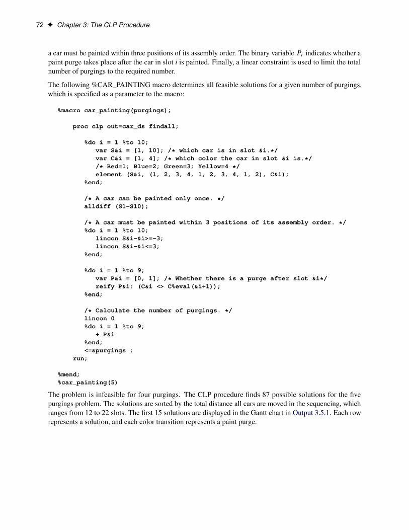
72 F Chapter 3: The CLP Procedure
a car must be painted within three positions of its assembly order. The binary variable Pi indicates whether apaint purge takes place after the car in slot i is painted. Finally, a linear constraint is used to limit the totalnumber of purgings to the required number.
The following %CAR_PAINTING macro determines all feasible solutions for a given number of purgings,which is specified as a parameter to the macro:
%macro car_painting(purgings);
proc clp out=car_ds findall;
%do i = 1 %to 10;var S&i = [1, 10]; /* which car is in slot &i.*/var C&i = [1, 4]; /* which color the car in slot &i is.*//* Red=1; Blue=2; Green=3; Yellow=4 */element (S&i, (1, 2, 3, 4, 1, 2, 3, 4, 1, 2), C&i);
%end;
/* A car can be painted only once. */alldiff (S1-S10);
/* A car must be painted within 3 positions of its assembly order. */%do i = 1 %to 10;
lincon S&i-&i>=-3;lincon S&i-&i<=3;
%end;
%do i = 1 %to 9;var P&i = [0, 1]; /* Whether there is a purge after slot &i*/reify P&i: (C&i <> C%eval(&i+1));
%end;
/* Calculate the number of purgings. */lincon 0%do i = 1 %to 9;
+ P&i%end;<=&purgings ;
run;
%mend;%car_painting(5)
The problem is infeasible for four purgings. The CLP procedure finds 87 possible solutions for the fivepurgings problem. The solutions are sorted by the total distance all cars are moved in the sequencing, whichranges from 12 to 22 slots. The first 15 solutions are displayed in the Gantt chart in Output 3.5.1. Each rowrepresents a solution, and each color transition represents a paint purge.

Example 3.6: Scene Allocation Problem F 73
Output 3.5.1 Car Painting Schedule with Five Purgings
Example 3.6: Scene Allocation ProblemThe scene allocation problem consists of deciding when to shoot each scene of a movie in order to minimizethe total production cost (Van Hentenryck 2002). Each scene involves a number of actors, and at most fivescenes a day can be shot. All actors who appear in a scene must be present on the day the scene is shot. Eachactor has a daily rate for each day spent in the studio, regardless of the number of scenes in which he or sheappears on that day. The goal is to minimize the production costs of the studio.
The actor names, daily fees, and the scenes they appear are given in the SCENE data set shown in Output 3.6.1.The variables S_Var1, . . . , S_Var9 indicate the scenes in which the actor appears. For example, the first

74 F Chapter 3: The CLP Procedure
observation indicates that Patt’s daily fee is 26,481 and that Patt appears in scenes 2, 5, 7, 10, 11, 13, 15, and17.
Output 3.6.1 The Scene Data Set
Obs Number Actor DailyFee S_Var1 S_Var2 S_Var3 S_Var4 S_Var5 S_Var6 S_Var7 S_Var8 S_Var9
1 1 Patt 26481 2 5 7 10 11 13 15 17 .
2 2 Casta 25043 4 7 9 10 13 16 19 . .
3 3 Scolaro 30310 3 6 9 10 14 16 17 18 .
4 4 Murphy 4085 2 8 12 13 15 . . . .
5 5 Brown 7562 2 3 12 17 . . . . .
6 6 Hacket 9381 1 2 12 13 18 . . . .
7 7 Anderson 8770 5 6 14 . . . . . .
8 8 McDougal 5788 3 5 6 9 10 12 15 16 18
9 9 Mercer 7423 3 4 5 8 9 16 . . .
10 10 Spring 3303 5 6 . . . . . . .
11 11 Thompson 9593 6 9 12 15 18 . . . .
There are 19 scenes and at most five scenes can be filmed in one day, so at least four days are needed toschedule all the scenes (d19
5e D 4). Let Sj_k be a binary variable that equals 1 if scene j is shot on day k.
Let Ai_k be another binary variable that equals 1 if actor i is present on day k. The variable Namei is thename of the ith actor; Costi is the daily cost of the ith actor. Ai_Sj D 1 if actor i appears in scene j, and 0otherwise.
The objective function representing the total production cost is given by
min11X
iD1
4XkD1
Costi � Ai_k
The %SCENE macro first reads the data set scene and produces three sets of macro variables: Namei , Costi ,and Ai_Sj . The data set cost is created next to specify the objective function. Finally, the CLP procedure isinvoked. There are two sets of GCC constraints in the CLP call: one to make sure each scene is shot exactlyonce, and one to limit the number of scenes shot per day to be at least four and at most five. There are twosets of LINCON constraints: one to indicate that an actor must be present if any of his or her scenes are shotthat day, and one for breaking symmetries to improve efficiency. Additionally, an OBJ statement specifiesupper and lower bounds on the objective function to be minimized.
%macro scene;/* Ai_Sj=1 if actor i appears in scene j *//* Ai_Sj=0 otherwise *//* Initialize to 0 */%do i=1 %to 11; /* 11 actors */
%do j=1 %to 19; /* 19 scenes */%let A&i._S&j=0;
%end;%end;
data scene_cost;set scene;keep DailyFee A;

Example 3.6: Scene Allocation Problem F 75
retain DailyFee A;do day=1 to 4;
A='A'||left(strip(_N_))||'_'||left(strip(day));output;
end;call symput("Name"||strip(_n_), Actor); /* read actor name */call symput("Cost"||strip(_n_), DailyFee); /* read actor cost *//* read whether an actor appears in a scene */%do i=1 %to 9; /* 9 scene variables in the data set */
if S_Var&i > 0 thencall symput("A"||strip(_n_)||"_S"||strip(S_Var&i), 1);
%end;run;/* Create constraint data set which defines the objective function */proc transpose data=scene_cost out=cost(drop=_name_);
var DailyFee;id A;
run;data cost;
set cost;_TYPE_='MIN';_RHS_=.;
run;
/* Find the minimum objective value. */proc clp condata=cost out=out varselect=maxc;
/* Set lower and upper bounds for the objective value *//* Lower bound: every actor appears on one day. *//* Upper bound: every actor appears on all four days. */obj lb=137739 ub=550956;
/* Declare variables. */%do k=1 %to 4; /* 4 days */%do j=1 %to 19; /* 19 scenes */
var S&j._&k=[0,1]; /* Indicates if scene j is shot on day k. */%end;%do i=1 %to 11; /* 11 actors */
var A&i._&k=[0,1]; /* Indicates if actor i is present on day k.*/%end;%end;
/* Every scene is shot exactly once.*/%do j=1 %to 19;
gcc (%do k=1 %to 4;
S&j._&k%end;)=( (1, 1, 1) );
%end;
/* At least 4 and at most 5 scenes are shot per day. */%do k=1 %to 4;
gcc (%do j=1 %to 19;

76 F Chapter 3: The CLP Procedure
S&j._&k%end;)=( (1, 4, 5) );
%end;
/* Actors for a scene must be present on day of shooting.*/%do k=1 %to 4;
%do j=1 %to 19;%do i=1 %to 11;
%if (&&A&i._S&j>0) %then %do;lincon S&j._&k <= A&i._&k;
%end;%end;
%end;%end;
/* Symmetry breaking constraints. Without loss of any generality, we *//* can assume Scene1 to be shot on day 1, Scene2 to be shot on day 1 *//* or day 2, and Scene3 to be shot on either day 1, day 2 or day 3. */lincon S1_1 = 1, S1_2 = 0, S1_3 = 0, S1_4 = 0,
S2_3 = 0, S2_4 = 0, S3_4 = 0;
/* If Scene2 is shot on day 1, *//* then Scene3 can be shot on day 1 or day 2. */lincon S2_1 + S3_3 <= 1;
run;%put &_ORCLP_;
%mend scene;
The optimal production cost is 334,144, as reported in the _ORCLP_ macro variable. The correspondingactor schedules and scene schedules are displayed in Output 3.6.2 and Output 3.6.3, respectively.

Example 3.6: Scene Allocation Problem F 77
Output 3.6.2 Scene Allocation Problem: Actor Schedules
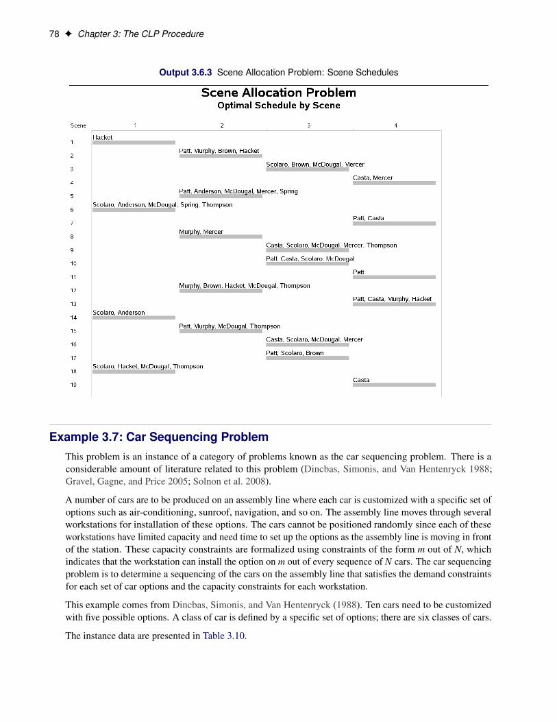
78 F Chapter 3: The CLP Procedure
Output 3.6.3 Scene Allocation Problem: Scene Schedules
Example 3.7: Car Sequencing ProblemThis problem is an instance of a category of problems known as the car sequencing problem. There is aconsiderable amount of literature related to this problem (Dincbas, Simonis, and Van Hentenryck 1988;Gravel, Gagne, and Price 2005; Solnon et al. 2008).
A number of cars are to be produced on an assembly line where each car is customized with a specific set ofoptions such as air-conditioning, sunroof, navigation, and so on. The assembly line moves through severalworkstations for installation of these options. The cars cannot be positioned randomly since each of theseworkstations have limited capacity and need time to set up the options as the assembly line is moving in frontof the station. These capacity constraints are formalized using constraints of the form m out of N, whichindicates that the workstation can install the option on m out of every sequence of N cars. The car sequencingproblem is to determine a sequencing of the cars on the assembly line that satisfies the demand constraintsfor each set of car options and the capacity constraints for each workstation.
This example comes from Dincbas, Simonis, and Van Hentenryck (1988). Ten cars need to be customizedwith five possible options. A class of car is defined by a specific set of options; there are six classes of cars.
The instance data are presented in Table 3.10.

Example 3.7: Car Sequencing Problem F 79
Table 3.10 The Instance Data
Option Capacity Car ClassName Type m/N 1 2 3 4 5 6
Option 1 1 1/2 1 0 0 0 1 1Option 2 2 2/3 0 0 1 1 0 1Option 3 3 1/3 1 0 0 0 1 0Option 4 4 2/5 1 1 0 1 0 0Option 5 5 1/5 0 0 1 0 0 0
Number of Cars 1 1 2 2 2 2
For example, car class 4 requires installation of option 2 and option 4, and two cars of this class are required.The workstation for option 2 can process only two out of every sequence of three cars. The workstation foroption 4 has even less capacity—two out of every five cars.
The instance data for this problem is used to create a SAS data set, which in turn is processed to generate theSAS macro variables shown in Table 3.11 that are used in the CLP procedure. The assembly line is treated asa sequence of slots, and each car must be allocated to a single slot.
Table 3.11 SAS Macro Variables
Macro Variable Description Value
Ncars Number of cars (slots) 10
Nops Number of options 5
Nclss Number of classes 6
Max_1–Max_5 For each option, the maximum num-ber of cars with that option in a block
1 2 1 2 1
Blsz_1–Blsz_5 For each option, the block size towhich the maximum number refers
2 3 3 5 5
class_1–class_6 Index number of each class 1 2 3 4 5 6
cars_cls_1–cars_cls_6 Number of cars in each class 1 1 2 2 2 2
list_1–list_5 Class indicator list for each option;for example, classes 1, 5, and 6 thatrequire option 1 (list_1)
list_1=1,0,0,0,1,1list_2=0,0,1,1,0,1list_3=1,0,0,0,1,0list_4=1,1,0,1,0,0list_5=0,0,1,0,0,0
cars_opts_1–cars_opts_5 Number of cars for each option(cars_opts_1 represents the numberof cars that require option 1)
5 6 3 4 2
The decision variables for this problem are shown in Table 3.12.

80 F Chapter 3: The CLP Procedure
Table 3.12 The Decision Variables
Variable Definition Description
S_1–S_10=[1,6] S_i is the class of cars as-signed to slot i.
O_1_1–O_1_5=[0,1]. . . O_10_1–O_10_5=[0,1]
O_i_j=1 if the class assignedto slot i needs option j.
In the following SAS statements, the workstation capacity constraints are expressed using a set of linearconstraints for each workstation. The demand constraints for each car class are expressed using a single GCCconstraint. The relationships between slot variables and option variables are expressed using an elementconstraint for each option variable. Finally, a set of redundant constraints are introduced to improve theefficiency of propagation. The idea behind the redundant constraint is the following realization: if theworkstation for option j has capacity r out of s, then at most r cars in the sequence .n� sC1/; : : : ; n can haveoption j where n is the total number of cars. Consequently at least nj � r cars in the sequence 1; : : : ; n � smust have option j, where nj is the number of cars with option j. Generalizing this further, at least nj � k � r
cars in the sequence 1; : : : ; .n � k � s/ must have option j, k D 1; : : : ; bn=sc.
%macro car_sequencing(outdata);
proc clp out=&outdata varselect=minrmaxc findall;
/* Declare Variables */var
/* Slot variables: Si - class of car assigned to Slot i */%do i = 1 %to &Ncars;
S_&i = [1, &Nclss]%end;
/* Option variables: Oij- indicates if class assigned to Sloti needs Option j */
%do i = 1 %to &Ncars;%do j = 1 %to &Nops;
O_&i._&j = [0, 1]%end;
%end;;
/* Capacity Constraints: for each option j *//* Installed in at most Max_j cars out of every sequence of BlSz_j cars */%do j = 1 %to &Nops;
%do i = 0 %to %eval(&Ncars-&&BlSz_&j);lincon 0%do k=1 %to &&BlSz_&j;
+ O_%eval(&i+&k)_&j%end;<=&&Max_&j;
%end;%end;
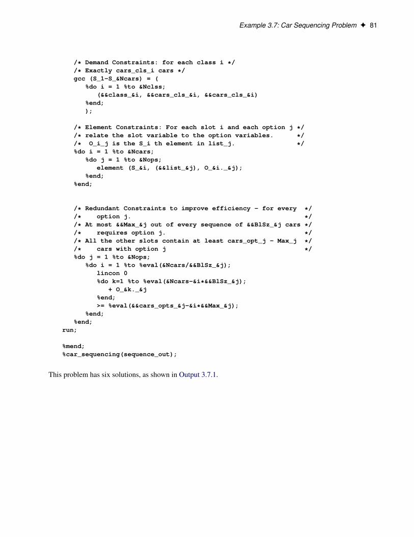
Example 3.7: Car Sequencing Problem F 81
/* Demand Constraints: for each class i *//* Exactly cars_cls_i cars */gcc (S_1-S_&Ncars) = (
%do i = 1 %to &Nclss;(&&class_&i, &&cars_cls_&i, &&cars_cls_&i)
%end;);
/* Element Constraints: For each slot i and each option j *//* relate the slot variable to the option variables. *//* O_i_j is the S_i th element in list_j. */%do i = 1 %to &Ncars;
%do j = 1 %to &Nops;element (S_&i, (&&list_&j), O_&i._&j);
%end;%end;
/* Redundant Constraints to improve efficiency - for every *//* option j. *//* At most &&Max_&j out of every sequence of &&BlSz_&j cars *//* requires option j. *//* All the other slots contain at least cars_opt_j - Max_j *//* cars with option j */%do j = 1 %to &Nops;
%do i = 1 %to %eval(&Ncars/&&BlSz_&j);lincon 0%do k=1 %to %eval(&Ncars-&i*&&BlSz_&j);
+ O_&k._&j%end;>= %eval(&&cars_opts_&j-&i*&&Max_&j);
%end;%end;
run;
%mend;%car_sequencing(sequence_out);
This problem has six solutions, as shown in Output 3.7.1.

82 F Chapter 3: The CLP Procedure
Output 3.7.1 Car Sequencing
Example 3.8: Round-Robin ProblemRound-robin tournaments (and variations of them) are a popular format in the scheduling of many sportsleague tournaments. In a single round-robin tournament, each team plays every other team just once. In adouble round-robin (DRR) tournament, each team plays every other team twice: once at home and onceaway.
This particular example deals with a single round-robin tournament by modeling it as a scheduling CSP.A special case of a double round-robin tournament can be found in Example 3.12, “Scheduling a MajorBasketball Conference” and features a different modeling approach.
Consider 14 teams that participate in a single round-robin tournament. Four rooms are provided for thetournament. Thus,
�142
�D 91 games and d91
4e D 23 time slots (rounds) need to be scheduled. Since each
game requires two teams, a room, and an available time slot, you can regard each game as an activity, the twoteams and the room as resources required by the activity, and the time slot as defined by the start and finishtimes of the activity.
In other words, you can treat this as a scheduling CSP with activities ACT_i_j where i < j , and resourcesTEAM1 through TEAM14 and ROOM1 through ROOM4. For a given i and j, activity ACT_i_j requires theresources TEAMi, TEAMj, and one of ROOM1 through ROOM4. The resulting start time for activity A_i_jis the time slot for the game between TEAMi and TEAMj and the assigned ROOM is the venue for the game.

Example 3.8: Round-Robin Problem F 83
The following SAS macro, %ROUND_ROBIN, uses the CLP procedure to solve this problem. The%ROUND_ROBIN macro uses the number of teams as a parameter.
The ACTDATA= data set defines all activities ACT_i_j with duration one. The RESOURCE statementdeclares the TEAM and ROOM resources. The REQUIRES statement defines the resource requirements foreach activity ACT_i_j. The SCHEDULE statement defines the activity selection strategy as MINLS, whichselects an activity with minimum late start time from the set of activities that begin prior to the earliest earlyfinish time.
%macro round_robin(nteams);
%let nrounds = %eval(%sysfunc(ceil((&nteams * (&nteams - 1)/2)/4)));
data actdata;do i = 1 to &nteams - 1;
do j = i + 1 to &nteams;_activity_ = compress('ACT_'||put(i,best.)||'_'||put(j,best.));_duration_ = 1;output;
end;end;
run;
proc clp actdata = actdata schedule = schedule;schedule finish = &nrounds actselect=minls;resource (TEAM1-TEAM&nteams);resource (ROOM1-ROOM4);requires
%do i = 1 %to &nteams - 1;%do j = &i + 1 %to &nteams;
ACT_&i._&j = ( TEAM&i )ACT_&i._&j = ( TEAM&j )ACT_&i._&j = ( ROOM1, ROOM2, ROOM3, ROOM4)
%end;%end;
;run;
proc sort data=schedule;by start finish;
run;
%mend round_robin;
%round_robin(14);
The resulting team schedule is displayed in Output 3.8.1. The vertical axis lists the teams, and the horizontalaxis indicates the time slot of each game. The color of the bar indicates the room the game is played in, whilethe text above each bar identifies the opponent.

84 F Chapter 3: The CLP Procedure
Output 3.8.1 Round Robin Team Schedule
Another view of the complete schedule is the room schedule, which is shown in Output 3.8.2. The verticalaxis lists each room, and the horizontal axis indicates the time slot of each game. The numbers inside eachbar identify the team pairings for the corresponding room and time slot.

Example 3.9: Resource-Constrained Scheduling with Nonstandard Temporal Constraints F 85
Output 3.8.2 Round Robin Room Schedule
Example 3.9: Resource-Constrained Scheduling with Nonstandard TemporalConstraints
This example illustrates a real-life scheduling problem and is used as a benchmark problem in the constraintprogramming community. The problem is to schedule the construction of a five-segment bridge. (SeeOutput 3.9.1.) It comes from a Ph.D. dissertation on scheduling problems (Bartusch 1983).

86 F Chapter 3: The CLP Procedure
Output 3.9.1 The Bridge Problem
The project consists of 44 tasks and a set of constraints that relate these tasks. Table 3.13 displays the activityinformation, standard precedence constraints, and resource constraints. The sharing of a unary resource bymultiple activities results in the resource constraints being disjunctive in nature.
Table 3.13 Data for Bridge Construction
Activity Description Duration Predecessors Resource
pa Beginning of project 0a1 Bxcavation (abutment 1) 4 pa Excavatora2 Bxcavation (pillar 1) 2 pa Excavatora3 Bxcavation (pillar 2) 2 pa Excavatora4 Excavation (pillar 3) 2 pa Excavatora5 Excavation (pillar 4) 2 pa Excavatora6 Excavation (abutment 2) 5 pa Excavatorp1 Foundation piles 2 20 a3 Pile driverp2 Foundation piles 3 13 a4 Pile driverue Erection of temporary housing 10 pas1 Formwork (abutment 1) 8 a1 Carpentrys2 Formwork (pillar 1) 4 a2 Carpentry
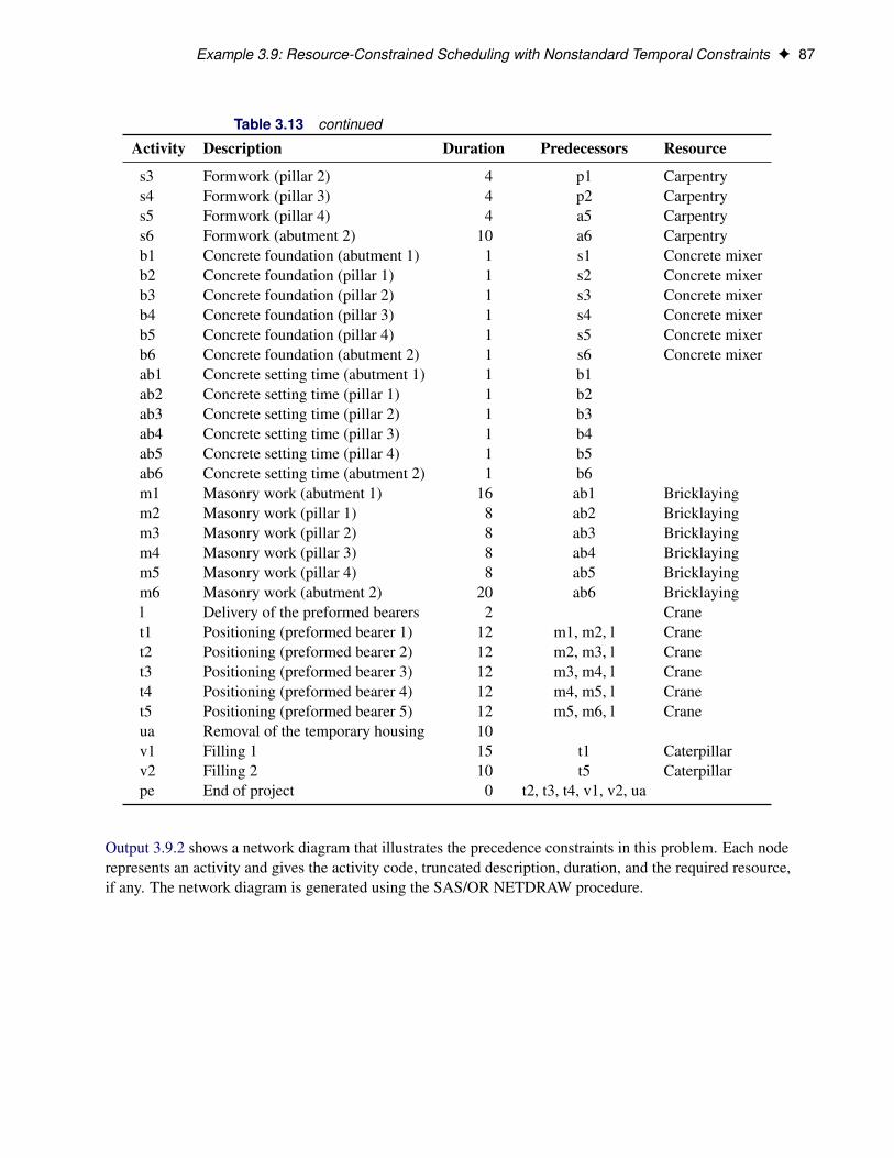
Example 3.9: Resource-Constrained Scheduling with Nonstandard Temporal Constraints F 87
Table 3.13 continued
Activity Description Duration Predecessors Resource
s3 Formwork (pillar 2) 4 p1 Carpentrys4 Formwork (pillar 3) 4 p2 Carpentrys5 Formwork (pillar 4) 4 a5 Carpentrys6 Formwork (abutment 2) 10 a6 Carpentryb1 Concrete foundation (abutment 1) 1 s1 Concrete mixerb2 Concrete foundation (pillar 1) 1 s2 Concrete mixerb3 Concrete foundation (pillar 2) 1 s3 Concrete mixerb4 Concrete foundation (pillar 3) 1 s4 Concrete mixerb5 Concrete foundation (pillar 4) 1 s5 Concrete mixerb6 Concrete foundation (abutment 2) 1 s6 Concrete mixerab1 Concrete setting time (abutment 1) 1 b1ab2 Concrete setting time (pillar 1) 1 b2ab3 Concrete setting time (pillar 2) 1 b3ab4 Concrete setting time (pillar 3) 1 b4ab5 Concrete setting time (pillar 4) 1 b5ab6 Concrete setting time (abutment 2) 1 b6m1 Masonry work (abutment 1) 16 ab1 Bricklayingm2 Masonry work (pillar 1) 8 ab2 Bricklayingm3 Masonry work (pillar 2) 8 ab3 Bricklayingm4 Masonry work (pillar 3) 8 ab4 Bricklayingm5 Masonry work (pillar 4) 8 ab5 Bricklayingm6 Masonry work (abutment 2) 20 ab6 Bricklayingl Delivery of the preformed bearers 2 Cranet1 Positioning (preformed bearer 1) 12 m1, m2, l Cranet2 Positioning (preformed bearer 2) 12 m2, m3, l Cranet3 Positioning (preformed bearer 3) 12 m3, m4, l Cranet4 Positioning (preformed bearer 4) 12 m4, m5, l Cranet5 Positioning (preformed bearer 5) 12 m5, m6, l Craneua Removal of the temporary housing 10v1 Filling 1 15 t1 Caterpillarv2 Filling 2 10 t5 Caterpillarpe End of project 0 t2, t3, t4, v1, v2, ua
Output 3.9.2 shows a network diagram that illustrates the precedence constraints in this problem. Each noderepresents an activity and gives the activity code, truncated description, duration, and the required resource,if any. The network diagram is generated using the SAS/OR NETDRAW procedure.

88 F Chapter 3: The CLP Procedure
Output 3.9.2 Network Diagram for the Bridge Construction Project
Brid
ge C
onst
ruct
ion
Pro
ject
pabe
ginn
in0ua
rem
oval
10l
deliv
ery
2cr
ane
ueer
ectio
n10a5
exca
vati
2ex
cava
to
a4ex
cava
ti2
exca
vato
a6ex
cava
ti5
exca
vato
a3ex
cava
ti2
exca
vato
a2ex
cava
ti2
exca
vato
a1ex
cava
ti4
exca
vato
s5fo
rmw
ork
4ca
rpen
tr
p2fo
unda
ti13
pile
dri
s6fo
rmw
ork
10ca
rpen
tr
p1fo
unda
ti20
pile
dri
s2fo
rmw
ork
4ca
rpen
tr
s1fo
rmw
ork
8ca
rpen
tr
b5co
ncre
te1
conc
rete
s4fo
rmw
ork
4ca
rpen
tr
b6co
ncre
te1
conc
rete
s3fo
rmw
ork
4ca
rpen
tr
b2co
ncre
te1
conc
rete
b1co
ncre
te1
conc
rete
ab5
conc
rete
1b4co
ncre
te1
conc
rete
ab6
conc
rete
1b3co
ncre
te1
conc
rete
ab2
conc
rete
1ab1
conc
rete
1
m5
mas
onry
8
bric
klay
ab4
conc
rete
1m6
mas
onry
20
bric
klay
ab3
conc
rete
1m2
mas
onry
8
bric
klay
m1
mas
onry
16
bric
klay
m4
mas
onry
8
bric
klay
t5po
sitio
n12
cran
e
m3
mas
onry
8
bric
klay
t1po
sitio
n12
cran
e
t4po
sitio
n12
cran
e
t3po
sitio
n12
cran
e
v2fil
ling
10ca
terp
il
t2po
sitio
n12
cran
e
v1fil
ling
15ca
terp
il
peen
d of
p0

Example 3.9: Resource-Constrained Scheduling with Nonstandard Temporal Constraints F 89
The following constraints are in addition to the standard precedence constraints:
1. The time between the completion of a particular formwork and the completion of its correspondingconcrete foundation is at most four days:
f .si/ � f .bi/ � 4; i D 1; � � � ; 6
2. There are at most three days between the end of a particular excavation (or foundation piles) and thebeginning of the corresponding formwork:
f .ai/ � s.si/ � 3; i D 1; 2; 5; 6
and
f .p1/ � s.s3/ � 3
f .p2/ � s.s4/ � 3
3. The formworks must start at least six days after the beginning of the erection of the temporary housing:
s.si/ � s.ue/C 6; i D 1; � � � ; 6
4. The removal of the temporary housing can start at most two days before the end of the last masonrywork:
s.ua/ � f .mi/ � 2; i D 1; � � � ; 6
5. The delivery of the preformed bearers occurs exactly 30 days after the beginning of the project:
s.l/ D s.pa/C 30
The following DATA step defines the data set bridge, which encapsulates all of the precedence constraintsand also indicates the resources that are required by each activity. Note the use of the reserved variables_ACTIVITY_, _SUCCESSOR_, _LAG_, and _LAGDUR_ to define the activity and precedence relationships.The list of reserved variables can be found in Table 3.6. The latter two variables are required for thenonstandard precedence constraints listed previously.

90 F Chapter 3: The CLP Procedure
data bridge;format _ACTIVITY_ $3. _DESC_ $34. _RESOURCE_ $14.
_SUCCESSOR_ $3. _LAG_ $3. ;input _ACTIVITY_ & _DESC_ & _DURATION_ _RESOURCE_ &
_SUCCESSOR_ & _LAG_ & _LAGDUR_;_QTY_ = 1;datalines;
a1 excavation (abutment 1) 4 excavator s1 . .a2 excavation (pillar 1) 2 excavator s2 . .a3 excavation (pillar 2) 2 excavator p1 . .a4 excavation (pillar 3) 2 excavator p2 . .a5 excavation (pillar 4) 2 excavator s5 . .a6 excavation (abutment 2) 5 excavator s6 . .ab1 concrete setting time (abutment 1) 1 . m1 . .ab2 concrete setting time (pillar 1) 1 . m2 . .ab3 concrete setting time (pillar 2) 1 . m3 . .ab4 concrete setting time (pillar 3) 1 . m4 . .ab5 concrete setting time (pillar 4) 1 . m5 . .ab6 concrete setting time (abutment 2) 1 . m6 . .b1 concrete foundation (abutment 1) 1 concrete mixer ab1 . .b1 concrete foundation (abutment 1) 1 concrete mixer s1 ff -4b2 concrete foundation (pillar 1) 1 concrete mixer ab2 . .b2 concrete foundation (pillar 1) 1 concrete mixer s2 ff -4b3 concrete foundation (pillar 2) 1 concrete mixer ab3 . .b3 concrete foundation (pillar 2) 1 concrete mixer s3 ff -4b4 concrete foundation (pillar 3) 1 concrete mixer ab4 . .b4 concrete foundation (pillar 3) 1 concrete mixer s4 ff -4b5 concrete foundation (pillar 4) 1 concrete mixer ab5 . .b5 concrete foundation (pillar 4) 1 concrete mixer s5 ff -4b6 concrete foundation (abutment 2) 1 concrete mixer ab6 . .b6 concrete foundation (abutment 2) 1 concrete mixer s6 ff -4l delivery of the preformed bearers 2 crane t1 . .l delivery of the preformed bearers 2 crane t2 . .l delivery of the preformed bearers 2 crane t3 . .l delivery of the preformed bearers 2 crane t4 . .l delivery of the preformed bearers 2 crane t5 . .m1 masonry work (abutment 1) 16 bricklaying t1 . .m1 masonry work (abutment 1) 16 bricklaying ua fs -2m2 masonry work (pillar 1) 8 bricklaying t1 . .m2 masonry work (pillar 1) 8 bricklaying t2 . .m2 masonry work (pillar 1) 8 bricklaying ua fs -2m3 masonry work (pillar 2) 8 bricklaying t2 . .m3 masonry work (pillar 2) 8 bricklaying t3 . .m3 masonry work (pillar 2) 8 bricklaying ua fs -2m4 masonry work (pillar 3) 8 bricklaying t3 . .m4 masonry work (pillar 3) 8 bricklaying t4 . .m4 masonry work (pillar 3) 8 bricklaying ua fs -2m5 masonry work (pillar 4) 8 bricklaying t4 . .m5 masonry work (pillar 4) 8 bricklaying t5 . .m5 masonry work (pillar 4) 8 bricklaying ua fs -2m6 masonry work (abutment 2) 20 bricklaying t5 . .m6 masonry work (abutment 2) 20 bricklaying ua fs -2p1 foundation piles 2 20 pile driver s3 . .

Example 3.9: Resource-Constrained Scheduling with Nonstandard Temporal Constraints F 91
p2 foundation piles 3 13 pile driver s4 . .pa beginning of project 0 . a1 . .pa beginning of project 0 . a2 . .pa beginning of project 0 . a3 . .pa beginning of project 0 . a4 . .pa beginning of project 0 . a5 . .pa beginning of project 0 . a6 . .pa beginning of project 0 . l fse 30pa beginning of project 0 . ue . .pe end of project 0 . . . .s1 formwork (abutment 1) 8 carpentry b1 . .s1 formwork (abutment 1) 8 carpentry a1 sf -3s2 formwork (pillar 1) 4 carpentry b2 . .s2 formwork (pillar 1) 4 carpentry a2 sf -3s3 formwork (pillar 2) 4 carpentry b3 . .s3 formwork (pillar 2) 4 carpentry p1 sf -3s4 formwork (pillar 3) 4 carpentry b4 . .s4 formwork (pillar 3) 4 carpentry p2 sf -3s5 formwork (pillar 4) 4 carpentry b5 . .s5 formwork (pillar 4) 4 carpentry a5 sf -3s6 formwork (abutment 2) 10 carpentry b6 . .s6 formwork (abutment 2) 10 carpentry a6 sf -3t1 positioning (preformed bearer 1) 12 crane v1 . .t2 positioning (preformed bearer 2) 12 crane pe . .t3 positioning (preformed bearer 3) 12 crane pe . .t4 positioning (preformed bearer 4) 12 crane pe . .t5 positioning (preformed bearer 5) 12 crane v2 . .ua removal of the temporary housing 10 . pe . .ue erection of temporary housing 10 . . . .ue erection of temporary housing 10 . s1 ss 6ue erection of temporary housing 10 . s2 ss 6ue erection of temporary housing 10 . s3 ss 6ue erection of temporary housing 10 . s4 ss 6ue erection of temporary housing 10 . s5 ss 6ue erection of temporary housing 10 . s6 ss 6v1 filling 1 15 caterpillar pe . .v2 filling 2 10 caterpillar pe . .;
The CLP procedure is then invoked by using the following statements with the SCHEDTIME= option.
/* invoke PROC CLP */proc clp actdata=bridge schedtime=schedtime_bridge;
schedule finish=104;run;
The FINISH= option is specified to find a solution in 104 days, which also happens to be the optimalmakespan.

92 F Chapter 3: The CLP Procedure
The schedtime_bridge data set contains the activity start and finish times as computed by the CLP procedure.Since an activity gets assigned to at most one resource, it is possible to represent the complete scheduleinformation more concisely by merging the schedtime_bridge data set with the bridge_info data set, as shownin the following statements.
/* Create Consolidated Schedule */proc sql;
create table bridge_info asselect distinct _ACTIVITY_ as ACTIVITY format $3. length 3,_DESC_ as DESCRIPTION, _RESOURCE_ as RESOURCE from bridge;
proc sort data=schedtime_bridge;by ACTIVITY;
run;
data schedtime_bridge;merge bridge_info schedtime_bridge;by ACTIVITY;
run;
proc sort data=schedtime_bridge;by START FINISH;
run;
proc print data=schedtime_bridge noobs width=min;;title 'Bridge Construction Schedule';
run;
Output 3.9.3 shows the resulting merged data set.

Example 3.9: Resource-Constrained Scheduling with Nonstandard Temporal Constraints F 93
Output 3.9.3 Bridge Construction Schedule
Bridge Construction ScheduleBridge Construction Schedule
ACTIVITY DESCRIPTION RESOURCE SOLUTION DURATION START FINISH
pa beginning of project 1 0 0 0
a4 excavation (pillar 3) excavator 1 2 0 2
ue erection of temporary housing 1 10 0 10
a5 excavation (pillar 4) excavator 1 2 2 4
p2 foundation piles 3 pile driver 1 13 2 15
a2 excavation (pillar 1) excavator 1 2 5 7
s5 formwork (pillar 4) carpentry 1 4 6 10
a3 excavation (pillar 2) excavator 1 2 7 9
b5 concrete foundation (pillar 4) concrete mixer 1 1 10 11
s2 formwork (pillar 1) carpentry 1 4 10 14
ab5 concrete setting time (pillar 4) 1 1 11 12
a1 excavation (abutment 1) excavator 1 4 12 16
m5 masonry work (pillar 4) bricklaying 1 8 12 20
b2 concrete foundation (pillar 1) concrete mixer 1 1 14 15
ab2 concrete setting time (pillar 1) 1 1 15 16
s4 formwork (pillar 3) carpentry 1 4 15 19
p1 foundation piles 2 pile driver 1 20 15 35
b4 concrete foundation (pillar 3) concrete mixer 1 1 19 20
a6 excavation (abutment 2) excavator 1 5 19 24
s1 formwork (abutment 1) carpentry 1 8 19 27
ab4 concrete setting time (pillar 3) 1 1 20 21
m2 masonry work (pillar 1) bricklaying 1 8 20 28
b1 concrete foundation (abutment 1) concrete mixer 1 1 27 28
s6 formwork (abutment 2) carpentry 1 10 27 37
ab1 concrete setting time (abutment 1) 1 1 28 29
m4 masonry work (pillar 3) bricklaying 1 8 28 36
l delivery of the preformed bearers crane 1 2 30 32
t4 positioning (preformed bearer 4) crane 1 12 36 48
m1 masonry work (abutment 1) bricklaying 1 16 36 52
b6 concrete foundation (abutment 2) concrete mixer 1 1 37 38
s3 formwork (pillar 2) carpentry 1 4 37 41
ab6 concrete setting time (abutment 2) 1 1 38 39
b3 concrete foundation (pillar 2) concrete mixer 1 1 41 42
ab3 concrete setting time (pillar 2) 1 1 42 43
m3 masonry work (pillar 2) bricklaying 1 8 52 60
t1 positioning (preformed bearer 1) crane 1 12 52 64
m6 masonry work (abutment 2) bricklaying 1 20 60 80
t2 positioning (preformed bearer 2) crane 1 12 64 76
v1 filling 1 caterpillar 1 15 64 79
ua removal of the temporary housing 1 10 78 88
t5 positioning (preformed bearer 5) crane 1 12 80 92
v2 filling 2 caterpillar 1 10 92 102
t3 positioning (preformed bearer 3) crane 1 12 92 104
pe end of project 1 0 104 104

94 F Chapter 3: The CLP Procedure
A Gantt chart of the schedule in Output 3.9.3, produced using the SAS/OR GANTT procedure, is displayedin Output 3.9.4. Each activity bar is color coded according to the resource associated with it. The legendidentifies the name of the resource that is associated with each color.
Example 3.10: Scheduling with Alternate ResourcesThis example shows an interesting job shop scheduling problem that illustrates the use of alternative resources.There are 90 jobs (J1–J90), each taking either one or two days, that need to be processed on one of tenmachines (M0–M9). Not every machine can process every job. In addition, certain jobs also require one ofseven operators (OP0–OP6). As with the machines, not every operator can be assigned to every job. Thereare no explicit precedence relationships in this example.
The machine and operator requirements for each job are shown in Output 3.10.1. Each row in the graphdefines a resource requirement for up to three jobs that are identified in the columns Jb1–Jb3 to the left ofthe chart. The horizontal axis of the chart represents the resources and is split into two regions by a verticalline. The resources to the left of the divider are the machines, Mach0–Mach9, and the resources to the rightof the divider are the operators, Oper0–Oper6. For each row on the chart, a bar on the chart represents apotential requirement for the corresponding resource listed above.
Each of the jobs listed in columns Jb1–Jb3 can be processed on one of the machines in Mach0–Mach9 andrequires the assistance of one of the operators in Oper0–Oper6 while being processed. An eligible resourceis represented by a bar, and the length of the bar indicates the duration of the job.
For example, row five specifies that job number 7 can be processed on machine 6, 7, or 8 and additionallyrequires either operator 5 or operator 6 in order to be processed. The next row indicates that jobs 8 and 9 canalso be processed on the same set of machines. However, they do not require any operator assistance.

Example 3.10: Scheduling with Alternate Resources F 95
Output 3.9.4 Gantt Chart for the Bridge Construction Project
PR
OC
CLP
- S
olut
ion
to B
ridge
Pro
blem
:104
day
s (o
ptim
al)
N/A
bri
ckla
ying
car
pent
ry
cat
erpi
llar
con
cret
e m
ixer
cra
ne
exc
avat
or
pile
dri
ver
Res
ourc
e U
sed
05
10
15
20
25
30
35
40
45
50
55
60
65
70
75
80
85
90
95
10
01
05
Act
Sta
rtF
inis
h
pa
0
0a
4
02
ue
0
10
a5
2
4p
2
21
5a
2
57
s5
6
10
a3
7
9b
5
10
11
s2
1
01
4a
b5
11
12
a1
1
21
6m
5
12
20
b2
1
41
5a
b2
15
16
s4
1
51
9p
1
15
35
b4
1
92
0a
6
19
24
s1
1
92
7a
b4
20
21
m2
2
02
8b
1
27
28
s6
2
73
7a
b1
28
29
m4
2
83
6l
30
32
t4
36
48
m1
3
65
2b
6
37
38
s3
3
74
1a
b6
38
39
b3
4
14
2a
b3
42
43
m3
5
26
0t1
5
26
4m
6
60
80
t2
64
76
v1
64
79
ua
7
88
8t5
8
09
2v2
9
21
02
t3
92
10
4p
e
10
41
04

96 F Chapter 3: The CLP Procedure
Output 3.10.1 Machine and Operator Requirements

Example 3.10: Scheduling with Alternate Resources F 97
The CLP procedure is invoked by using the following statements with FINISH=12 in the SCHEDULEstatement to obtain a 12-day solution that is also known to be optimal. In order to obtain the optimal solution,it is necessary to invoke the edge-finding consistency routines, which are activated with the EDGEFINDERoption in the SCHEDULE statement. The activity selection strategy is specified as DMINLS, which selectsthe activity with the earliest late start time. Activities with identical resource requirements are groupedtogether in the REQUIRES statement.
proc clp dom=[0,12] restarts=500 dpr=6 showprogressschedtime=schedtime_altres schedres=schedres_altres;schedule start=0 finish=12 actselect=dminls edgefinder;
activity (J1-J20 J24-J30 J34-J40 J48-J50 J54-J60J68-J70 J74-J80 J85-J90) = (1) /* one day jobs */(J21-J23 J31-J33 J41-J47 J51-J53 J61-J67J71-J73 J81-J84) = (2); /* two day jobs */
resource (M0-M9) (OP0-OP6);
requires/* machine requirements */(J85) = (M0)(J1 J20 J21 J22 J38 J39 J45 J46 J65 J66) = (M0, M1)(J19 J2 J58 J59 J60 J78 J79 J80) = (M0, M1, M2)(J86) = (M1)(J11) = (M1, M2)(J3) = (M1, M2, M3)(J23 J40 J87) = (M2)(J47 J48 J67 J68) = (M2, M3)(J30 J31 J88) = (M3)(J17 J18 J51 J52 J72 J73) = (M3, M4)(J4 J5 J6) = (M3, M4, M5)(J89) = (M4)(J28 J29 J32 J33 J49 J50 J69) = (M4, M5)(J70 J71 J90) = (M5)(J15 J16 J53 J54) = (M5, M6)(J26 J27 J34 J35 J41 J42 J61 J62 J74 J75 J81 J82) = (M6, M7)(J7 J8 J9) = (M6, M7, M8)(J10 J12 J13 J14 J55 J56 J57) = (M7, M8, M9)(J24 J25 J36 J37 J43 J44 J63 J64 J76 J77 J83 J84) = (M8, M9)/* operator requirements */(J53 J88) = (OP0)(J38 J39 J49 J50 J69 J70) = (OP0, OP1)(J1 J2 J21 J22 J23 J3 J71 J72 J73) = (OP0, OP1, OP2)(J11 J12 J13 J14) = (OP0, OP1, OP2, OP3)(J89) = (OP1)(J51 J52) = (OP1, OP2)(J40 J90) = (OP2)(J47 J48 J67 J68) = (OP2, OP3)(J4 J5 J6) = (OP2, OP3, OP4, OP5)(J85) = (OP3)(J29 J30 J31 J32 J58 J59 J78 J79) = (OP3, OP4)(J86) = (OP4)

98 F Chapter 3: The CLP Procedure
(J45 J46 J65 J66) = (OP4, OP5)(J15 J16 J17) = (OP4, OP5, OP6)(J87) = (OP5)(J27 J28 J33 J34 J60 J61 J7 J74 J80 J81) = (OP5, OP6)(J41 J54) = (OP6);
run;
The resulting schedule is shown in a series of Gantt charts that are displayed in Output 3.10.2 and Out-put 3.10.3. In each of these Gantt charts, the vertical axis lists the different jobs, the horizontal bar representsthe start and finish times for each of the jobs, and the text above each bar identifies the machine that thejob is being processed on. Output 3.10.2 displays the schedule for the operator-assisted tasks (one for eachoperator), while Output 3.10.3 shows the schedule for automated tasks (that is, those tasks that do not requireoperator intervention).
Output 3.10.2 Operator-Assisted Jobs Schedule

Example 3.10: Scheduling with Alternate Resources F 99
Output 3.10.2 continued

100 F Chapter 3: The CLP Procedure
Output 3.10.2 continued

Example 3.10: Scheduling with Alternate Resources F 101
Output 3.10.3 Automated Jobs Schedule
A more interesting Gantt chart is that of the resource schedule by machine, as shown in Output 3.10.4. Thischart displays the schedule for each machine. Every row corresponds to a machine. Every bar on each rowconsists of multiple segments, and every segment represents a job that is processed on the machine. Eachsegment is also coded according to the operator assigned to it. The mapping of the coding is indicated in thelegend. It is evident that the schedule is optimal since none of the machines or operators are idle at any timeduring the schedule.

102 F Chapter 3: The CLP Procedure
Output 3.10.4 Machine Schedule
Example 3.11: 10×10 Job Shop Scheduling ProblemThis example is a job shop scheduling problem from Lawrence (1984). This test is also known as LA19in the literature, and its optimal makespan is known to be 842 (Applegate and Cook 1991). There are 10jobs (J1–J10) and 10 machines (M0–M9). Every job must be processed on each of the 10 machines in apredefined sequence. The objective is to minimize the completion time of the last job to be processed, knownas the makespan. The jobs are described in the data set raw by using the following statements.
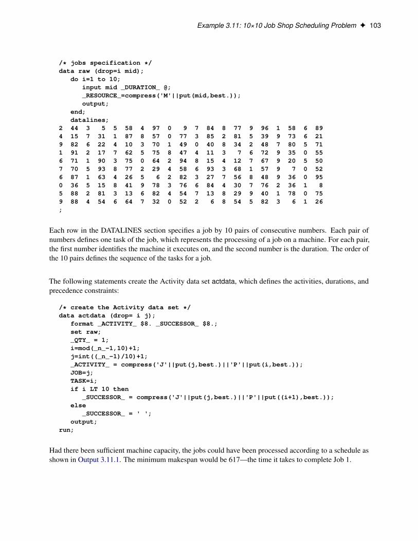
Example 3.11: 10×10 Job Shop Scheduling Problem F 103
/* jobs specification */data raw (drop=i mid);
do i=1 to 10;input mid _DURATION_ @;_RESOURCE_=compress('M'||put(mid,best.));output;
end;datalines;
2 44 3 5 5 58 4 97 0 9 7 84 8 77 9 96 1 58 6 894 15 7 31 1 87 8 57 0 77 3 85 2 81 5 39 9 73 6 219 82 6 22 4 10 3 70 1 49 0 40 8 34 2 48 7 80 5 711 91 2 17 7 62 5 75 8 47 4 11 3 7 6 72 9 35 0 556 71 1 90 3 75 0 64 2 94 8 15 4 12 7 67 9 20 5 507 70 5 93 8 77 2 29 4 58 6 93 3 68 1 57 9 7 0 526 87 1 63 4 26 5 6 2 82 3 27 7 56 8 48 9 36 0 950 36 5 15 8 41 9 78 3 76 6 84 4 30 7 76 2 36 1 85 88 2 81 3 13 6 82 4 54 7 13 8 29 9 40 1 78 0 759 88 4 54 6 64 7 32 0 52 2 6 8 54 5 82 3 6 1 26;
Each row in the DATALINES section specifies a job by 10 pairs of consecutive numbers. Each pair ofnumbers defines one task of the job, which represents the processing of a job on a machine. For each pair,the first number identifies the machine it executes on, and the second number is the duration. The order ofthe 10 pairs defines the sequence of the tasks for a job.
The following statements create the Activity data set actdata, which defines the activities, durations, andprecedence constraints:
/* create the Activity data set */data actdata (drop= i j);
format _ACTIVITY_ $8. _SUCCESSOR_ $8.;set raw;_QTY_ = 1;i=mod(_n_-1,10)+1;j=int((_n_-1)/10)+1;_ACTIVITY_ = compress('J'||put(j,best.)||'P'||put(i,best.));JOB=j;TASK=i;if i LT 10 then
_SUCCESSOR_ = compress('J'||put(j,best.)||'P'||put((i+1),best.));else
_SUCCESSOR_ = ' ';output;
run;
Had there been sufficient machine capacity, the jobs could have been processed according to a schedule asshown in Output 3.11.1. The minimum makespan would be 617—the time it takes to complete Job 1.

104 F Chapter 3: The CLP Procedure
Output 3.11.1 Gantt Chart: Schedule for the Unconstrained Problem
This schedule is infeasible when there is only a single instance of each machine. For example, at time period20, the schedule requires two instances of each of the machines M6, M7, and M9.
In order to solve the resource-constrained schedule, the CLP procedure is invoked by using the followingstatements:
proc clp domain=[0,842]actdata=actdataschedout=sched_jobshopdpr=50restarts=150showprogress;
schedule finish=842 edgefinder nf=1 nl=1;run;
The edge-finder algorithm is activated with the EDGEFINDER option in the SCHEDULE statement. Inaddition, the edge-finding extensions for detecting whether a job cannot be the first or cannot be the lastto be processed on a particular machine are invoked with the NF= and NL= options, respectively, in theSCHEDULE statement. The default activity selection and activity assignment strategies are used. A restartheuristic is used as the look-back method to handle recovery from failures. The DPR= option specifies that a

Example 3.12: Scheduling a Major Basketball Conference F 105
total restart be performed after encountering 50 failures, and the RESTARTS= option limits the number ofrestarts to 150.
The resulting 842-time-period schedule is displayed in Output 3.11.2. Each row represents a job. Eachsegment represents a task (the processing of a job on a machine), which is also coded according to theexecuting machine. The mapping of the coding is indicated in the legend. Note that no machine is used bymore than one job at any point in time.
Output 3.11.2 Gantt Chart: Optimal Resource-Constrained Schedule
Example 3.12: Scheduling a Major Basketball ConferenceExample 1.8 illustrated how you could use the CLP procedure to solve a single round-robin problem bymodeling it as a scheduling CSP. This example illustrates an alternate way of modeling and solving awell-known double round-robin problem using the CLP procedure. This example is based on the workof Nemhauser and Trick (1998) and deals with scheduling the Atlantic Coast Conference (ACC) Men’sBasketball games for the 1997–1998 season.
A temporally dense double round-robin (DDRR) for n teams is a double round-robin in which the n.n � 1/games are played over a minimal number of dates or time slots. If n is even, the number of slots is 2.n � 1/and each team plays in every time slot. If n is odd, the number of slots is 2n and .n � 1/ teams play in eachtime slot. In the latter case, each time slot has a team with a bye, and each team has two byes for the season.

106 F Chapter 3: The CLP Procedure
The Atlantic Coast Conference (ACC) 1997–1998 men’s basketball scheduling problem as described inNemhauser and Trick (1998) and Henz (2001) is a DDRR that consists of the following nine teams with theirabbreviated team name and team number shown in parentheses: Clemson (Clem 1), Duke (Duke 2), FloridaState (FSU 3), Georgia Tech (GT 4), Maryland (UMD 5), University of North Carolina (UNC 6), NC State(NCSU 7), Virginia (UVA 8), and Wake Forest (Wake 9).
The general objective is to schedule the DDRR to span the months of January and February and possiblyinclude a game in December or March or both. In general, each team plays twice a week—typicallyWednesday and Saturday. Although the actual day might differ, these two time slots are referred to as the“weekday slot” and the “weekend slot.” Since there are an odd number of teams, there is a team with a bye ineach slot and four games in each slot, resulting in a schedule that requires 18 time slots or nine weeks. Thelast time slot must be a weekend slot, which implies the first slot is a weekday slot. The first slot, denoted slot1, corresponds to the last weekday slot of December 1997, and the final slot, slot 18, corresponds to the firstweekend slot of March 1998. Each team plays eight home games and eight away games, and has two byes.
In addition there are several other constraints that must be satisfied. This example uses the following criteriaemployed by Nemhauser and Trick (1998) as presented by Henz (2001).
1. Mirroring: The dates are grouped into pairs .r1; r2/, such that each team gets to play against thesame team in dates r1 and r2 . Such a grouping is called a mirroring scheme. A separation of nineslots can be achieved by mirroring a round-robin schedule; while this separation is desirable, it is notpossible for this problem.
Nemhauser and Trick fix the mirroring scheme to
m D .1; 8/; .2; 9/; .3; 12/; .4; 13/; .5; 14/; .6; 15/; .7; 16/; .10; 17/; .11; 18/
in order to satisfy the constraints that UNC and Duke play in time slots 11 and 18. (See criterion 9.)
2. Initial and final home and away games: Every team must play at home on at least one of the firstthree dates. Every team must play at home on at least one of the last three dates. No team can playaway on both of the last two dates.
3. Home/away/bye pattern: No team can have more than two away games in a row. No team can havemore than two home games in a row. No team can have more than three away games or byes in a row.No team can have more than four home games or byes in a row.
4. Weekend pattern: Of the nine weekends, each team plays four at home, four away, and has one bye.
5. First weekends: Each team must have home games or byes on at least two of the first five weekends.
6. Rival matches: Every team except FSU has a traditional rival. The rival pairs are Clem-GT, Duke-UNC, UMD-UVA, and NCSU-Wake. In the last date, every team except FSU plays against its rival,unless it plays against FSU or has a bye.
7. Popular matches in February: The following pairings must occur at least once in dates 11 to 18:Duke-GT, Duke-Wake, GT-UNC, UNC-Wake.
8. Opponent sequence: No team plays in two consecutive away dates against Duke and UNC. No teamplays in three consecutive dates against Duke, UNC, and Wake (independent of the home or awaystatus).

Example 3.12: Scheduling a Major Basketball Conference F 107
9. Idiosyncrasies: UNC plays its rival Duke in the last date and in date 11. UNC plays Clem in thesecond date. Duke has a bye in date 16. Wake does not play home in date 17. Wake has a bye in thefirst date. Clem, Duke, UMD and Wake do not play away in the last date. Clem, FSU, and GT do notplay away in the first date. Neither FSU nor NCSU has a bye in last date. UNC does not have a bye inthe first date.
Previous work for solving round-robin problems, including that of Nemhauser and Trick (1998) and Henz(2001), have used a general three-phase framework for finding good schedules.
1. pattern generation
2. pattern set generation
3. timetable generation
A pattern is a valid sequence of home, away, and bye games for a given team for the entire season. Forexample, the following is a valid pattern:
A H B A H H A H A A H B H A A H H A
For this example, patterns that satisfy criterion 1 through criterion 5 and some constraints in criterion 9 aregenerated using the CLP procedure with the SAS macro %PATTERNS.
/****************************************************************//* First, find all possible patterns. Consider only time *//* constraints at this point. A pattern should be suitable *//* for any team. Do not consider individual teams yet. *//****************************************************************/%macro patterns();
proc clp out=all_patterns findall;/* For date 1 to 18. */%do j = 1 %to 18;
var h&j = [0, 1]; /* home */var a&j = [0, 1]; /* away */var b&j = [0, 1]; /* bye */
/* A team is either home, away, or bye. */lincon h&j + a&j + b&j=1;
%end;
/*------------------------------------------------------------*//* Criterion 1 - Mirroring Scheme *//*------------------------------------------------------------*//* The dates are grouped into pairs (j, j1), such that each *//* team plays the same opponent on dates j and j1. *//* A home game on date j will be an away game on date j1 */%do j = 1 %to 18;
%do j1 = %eval(&j+1) %to 18;%if ( &j=1 and &j1=8 ) or ( &j=2 and &j1=9 ) or
( &j=3 and &j1=12 ) or ( &j=4 and &j1=13 ) or( &j=5 and &j1=14 ) or ( &j=6 and &j1=15 ) or

108 F Chapter 3: The CLP Procedure
( &j=7 and &j1=16 ) or ( &j=10 and &j1=17 ) or( &j=11 and &j1=18 ) %thenlincon h&j = a&j1, a&j = h&j1, b&j = b&j1;;
%end;%end;
/*------------------------------------------------------------*//* Criterion 2 - Initial and Final Home and Away Games *//*------------------------------------------------------------*//* Every team must play home on at least one of the first three dates. */lincon h1 + h2 + h3 >= 1;
/* Every team must play home on at least one of the last three dates. */lincon h16 + h17 + h18 >= 1;
/* No team can play away on both last two dates. */lincon a17 + a18 < 2;
/*------------------------------------------------------------*//* Criterion 3 - Home/Away/Bye Pattern *//*------------------------------------------------------------*/%do j = 1 %to 16;
/* No team can have more than two away matches in a row.*/lincon a&j + a%eval(&j+1) + a%eval(&j+2) < 3;/* No team can have more than two home matches in a row.*/lincon h&j + h%eval(&j+1) + h%eval(&j+2) < 3;
%end;
/* No team can have more than three away matches or byes in a row.*/%do j = 1 %to 15;
lincon a&j + b&j + a%eval(&j+1) + b%eval(&j+1) + a%eval(&j+2)+ b%eval(&j+2) + a%eval(&j+3) + b%eval(&j+3) < 4;
%end;
/* No team can have more than four home matches or byes in a row.*/%do j = 1 %to 14;
lincon h&j + b&j + h%eval(&j+1) + b%eval(&j+1) + h%eval(&j+2)+ b%eval(&j+2) + h%eval(&j+3) + b%eval(&j+3) + h%eval(&j+4)+ b%eval(&j+4) < 5;
%end;
/*------------------------------------------------------------*//* Criterion 4 - Weekend Pattern *//*------------------------------------------------------------*//* Each team plays four weekends at home. */lincon 0 %do j = 2 %to 18 %by 2; +h&j %end; =4;/* Each team plays four weekends away. */lincon 0 %do j = 2 %to 18 %by 2; +a&j %end; =4;/* Each team has 1 weekend with a bye */lincon 0 %do j = 2 %to 18 %by 2; +b&j %end; =1;
/*------------------------------------------------------------*//* Criterion 5 - First Weekends *//*------------------------------------------------------------*/

Example 3.12: Scheduling a Major Basketball Conference F 109
/* Each team must have home games or byes on at least two *//* of the first five weekends. */lincon 0 %do j = 2 %to 10 %by 2; + h&j + b&j %end; >=2;
/*------------------------------------------------------------*//* Criterion 9 - (Partial) *//*------------------------------------------------------------*//* The team with a bye in date 1 does not play away on the *//* last date or home in date 17 (Wake) *//* The team with a bye in date 16 does not play away in *//* date 18 (Duke) */lincon b1 + a18 < 2, b1 + h17 < 2, b16 + a18 < 2;
run;
%mend;
%patterns;
The %PATTERNS macro generates 38 patterns. The next step is to find a subset of patterns with cardinalityequal to the number of teams that would collectively support a potential assignment to all of the teams. Forexample, each of the 18 time slots must correspond to four home games, four away games, and one bye.Furthermore, pairs of patterns that do not support a potential meeting date between the two correspondingteams are excluded. The following %PATTERN_SETS macro uses the CLP procedure with the precedingconstraints to generate 17 possible pattern sets.
/*****************************************************************//* Determine all possible "pattern sets" considering only time *//* constraints. *//* Individual teams are not considered at this stage. *//* xi - binary variable indicates pattern i is in pattern set *//*****************************************************************/
%macro pattern_sets();
data _null_;set all_patterns;%do i=1 %to 38;
if _n_=&i then do;%do j=1 %to 18;
call symput("h&i._&j", put(h&j,best.));call symput("a&i._&j", put(a&j,best.));call symput("b&i._&j", put(b&j,best.));
%end;end;
%end;run;
proc clp out=pattern_sets findall;/* xi=1 if pattern i belongs to pattern set */var (x1-x38)= [0, 1];
/* Exactly nine patterns per patterns set */

110 F Chapter 3: The CLP Procedure
lincon 0 %do i = 1 %to 38; + x&i %end;=9;
/* time slot constraints */%do j = 1 %to 18;
/* Four home games per time slot */lincon 0 %do i = 1 %to 38; + &&h&i._&j*x&i %end; =4;/* Four away games per time slot */lincon 0 %do i = 1 %to 38; + &&a&i._&j*x&i %end; =4;/* One bye per time slot */lincon 0 %do i = 1 %to 38; + &&b&i._&j*x&i %end; =1;
%end;
/* Exclude pattern pairs that do not support a meeting date */%do i = 1 %to 38;
%do i1 = %eval(&i+1) %to 38;%let count=0;%do j=1 %to 18;
%if ( (&&h&i._&j=0 or &&a&i1._&j=0) and(&&a&i._&j=0 or &&h&i1._&j=0)) %then %do;
%let count=%eval(&count+1);%end;
%end;%if (&count=18) %then %do;
lincon x&i+x&i1<=1;%end;
%end;%end;
run;
%mend;
%pattern_sets;
The %PATTERN_SETS macro generates 17 pattern sets. The final step is to add the individual teamconstraints and match up teams to the pattern set in order to come up with a schedule for each team. Theschedule for each team indicates the opponent for each time slot (0 for a bye) and whether it corresponds to ahome game, away game, or a bye.
The following SAS macro %TIMETABLE uses the pattern set index as a parameter and invokes the CLPprocedure with the individual team constraints to determine the team schedule.
/*********************************************************************//* Assign individual teams to pattern set k *//* Teams: 1 Clem, 2 Duke, 3 FSU, 4 GT, 5 UMD, 6 UNC, 7 NCSU, 8 UVA, *//* 9 Wake *//*********************************************************************/%macro timetable(k);
proc clp out=ACC_ds_&k varselect=minrmaxc findall;
%do j = 1 %to 18;/* alpha(i,j): Team i's opponent on date j ( 0 = bye ). */%do i = 1 %to 9;

Example 3.12: Scheduling a Major Basketball Conference F 111
var alpha&i._&j = [0, 9];%end;
/* Timetable constraint 1 *//* Opponents in a time slot must be distinct */alldiff ( %do i = 1 %to 9; alpha&i._&j %end; );
/* Timetable constraint 2 */%do i = 1 %to 9;
%do i1 = 1 %to 9;/* indicates if teams i and i1 play in time slot j */var X&i._&i1._&j = [0, 1];reify X&i._&i1._&j: (alpha&i._&j = &i1);
/* team i plays i1 iff team i1 plays i */%if (&i1 > &i ) %then %do;
lincon X&i._&i1._&j = X&i1._&i._&j;%end;
%end;%end;
%end;
/* Mirroring Scheme at team level. *//* The dates are grouped into pairs (j, j1) such that each *//* team plays the same opponent in dates j and j1. *//* One of these should be a home game for each team. */%do i = 1 %to 9;
%do j = 1 %to 18;%do j1 = %eval(&j+1) %to 18;
%if ( &j=1 and &j1=8 ) or ( &j=2 and &j1=9 ) or( &j=3 and &j1=12 ) or ( &j=4 and &j1=13 ) or( &j=5 and &j1=14 ) or ( &j=6 and &j1=15 ) or( &j=7 and &j1=16 ) or ( &j=10 and &j1=17 ) or( &j=11 and &j1=18 ) %then %do;lincon alpha&i._&j=alpha&i._&j1,/* H and A are matrices that indicate home *//* and away games */H&i._&j=A&i._&j1,H&i._&j1=A&i._&j;
%end;%end;
%end;%end;
/* Timetable constraint 3 *//* Each team plays every other team twice */%do i = 1 %to 9;
%do i1 = 1 %to 9;%if &i1 ne &i %then %do;
lincon 0 %do j = 1 %to 18; + X&i._&i1._&j %end; = 2;%end;
%end;%end;

112 F Chapter 3: The CLP Procedure
/* Timetable constraint 4 *//* Teams do not play against themselves */%do j = 1 %to 18;
%do i = 1 %to 9;lincon alpha&i._&j<>&i;lincon X&i._&i._&j = 0; /* redundant */
%end;%end;
/* Timetable constraint 5 *//* Setup Bye Matrix *//* alpha&i._&j=0 means team &i has a bye on date &j. */%do j = 1 %to 18;
%do i = 1 %to 9;var B&i._&j = [0, 1]; /*Bye matrix*/reify B&i._&j: ( alpha&i._&j = 0 );
%end;%end;
/* Timetable constraint 6 *//* alpha&i._&j=&i1 implies teams &i and &i1 play on date &j *//* It must be a home game for one, away game for the other */%do j = 1 %to 18;
%do i = 1 %to 9;%do i1 = 1 %to 9;
/* reify control variables.*/var U&i._&i1._&j = [0, 1] V&i._&i1._&j = [0, 1];
/* if &i is home and &i1 is away. */reify U&i._&i1._&j: ( H&i._&j + A&i1._&j = 2);/* if &i1 is home and &i is away. */reify V&i._&i1._&j: ( A&i._&j + H&i1._&j = 2);
/* Necessary condition if &i plays &i1 on date j */lincon X&i._&i1._&j <= U&i._&i1._&j + V&i._&i1._&j;
%end;%end;
%end;
/* Timetable constraint 7 *//* Each team must be home, away or have a bye on a given date */%do j = 1 %to 18;
%do i = 1 %to 9;/* Team &i is home (away) at date &j. */var H&i._&j = [0, 1] A&i._&j = [0, 1];lincon H&i._&j + A&i._&j + B&i._&j = 1;
%end;%end;
%do i = 1 %to 9;%do i1 = %eval(&i+1) %to 9;
/* Timetable constraint 8 */

Example 3.12: Scheduling a Major Basketball Conference F 113
/*-------------------------------------------------------*//* Criterion 6 - Rival Matches *//*-------------------------------------------------------*//* The final weekend is reserved for 'rival games' *//* unless the team plays FSU or has a bye */%if ( &i=1 and &i1=4 ) or ( &i=2 and &i1=6 ) or
( &i=5 and &i1=8 ) or ( &i=7 and &i1=9 ) %then %do;lincon X&i._&i1._18 + B&i._18 + X&i._3_18 = 1;
/* redundant */lincon X&i1._&i._18 + B&i1._18 + X&i1._3_18 = 1;
%end;
/* Timetable constraint 9 *//*-------------------------------------------------------*//* Criterion 7 - Popular Matches *//*-------------------------------------------------------*//* The following pairings are specified to occur at *//* least once in February. */%if ( &i=2 and &i1=4 ) or ( &i=2 and &i1=9 ) or
( &i=4 and &i1=6 ) or ( &i=6 and &i1=9 ) %then %do;lincon 0 %do j = 11 %to 18; + X&i._&i1._&j %end; >= 1;
/* redundant */lincon 0 %do j = 11 %to 18; + X&i1._&i._&j %end; >= 1;
%end;%end;
%end;
/* Timetable constraint 10 *//*-------------------------------------------------------*//* Criterion 8 - Opponent Sequence *//*-------------------------------------------------------*/%do i = 1 %to 9;
/* No team plays two consecutive away dates against *//* Duke (2) and UNC (6) */%do j = 1 %to 17;
var Q&i._26_&j = [0, 1] P&i._26_&j = [0, 1];reify Q&i._26_&j: ( X&i._2_&j + X&i._6_&j = 1 );reify P&i._26_&j: ( X&i._2_%eval(&j+1) + X&i._6_%eval(&j+1) =1 );lincon Q&i._26_&j + A&i._&j + P&i._26_&j + A&i._%eval(&j+1) < 4;
%end;
/* No team plays three consecutive dates against *//* Duke(2), UNC(6) and Wake(9). */%do j = 1 %to 16;
var L&i._269_&j = [0, 1] M&i._269_&j = [0, 1]N&i._269_&j = [0, 1];
reify L&i._269_&j: ( X&i._2_&j + X&i._6_&j + X&i._9_&j = 1 );reify M&i._269_&j: ( X&i._2_%eval(&j+1) + X&i._6_%eval(&j+1) +
X&i._9_%eval(&j+1) =1 );reify N&i._269_&j: ( X&i._2_%eval(&j+2) + X&i._6_%eval(&j+2) +
X&i._9_%eval(&j+2) =1 );lincon L&i._269_&j + M&i._269_&j + N&i._269_&j < 3;

114 F Chapter 3: The CLP Procedure
%end;%end;
/* Timetable constraint 11 *//*-------------------------------------------------------*//* Criterion 9 - Idiosyncratic Constraints *//*-------------------------------------------------------*//* UNC plays Duke in date 11 and 18 */lincon alpha6_11 = 2 ;lincon alpha6_18 = 2 ;/* UNC plays Clem in the second date. */lincon alpha6_2 = 1 ;/* Duke has a bye in date 16. */lincon B2_16 = 1 ;/* Wake does not play home in date 17. */lincon H9_17 = 0 ;/* Wake has a bye in the first date. */lincon B9_1 = 1 ;/* Clem, Duke, UMD and Wake do not play away in the last date. */lincon A1_18 = 0 ;lincon A2_18 = 0 ;lincon A5_18 = 0 ;lincon A9_18 = 0 ;/* Clem, FSU, and GT do not play away in the first date. */lincon A1_1 = 0 ;lincon A3_1 = 0 ;lincon A4_1 = 0 ;/* FSU and NCSU do not have a bye in the last date. */lincon B3_18 = 0 ;lincon B7_18 = 0 ;/* UNC does not have a bye in the first date. */lincon B6_1 = 0 ;
/* Timetable constraint 12 *//*-------------------------------------------------------*//* Match teams with patterns. *//*-------------------------------------------------------*/%do i = 1 %to 9; /* For each team */
var p&i=[1,9];%do j=1 %to 18; /* For each date */
element ( p&i, (&&col&k._h_&j), H&i._&j )( p&i, (&&col&k._a_&j), A&i._&j )( p&i, (&&col&k._b_&j), B&i._&j );
%end;%end;
run;
%mend;
/**************************************************************//* Try all possible pattern sets to find all valid schedules. *//**************************************************************/

Example 3.13: Balanced Incomplete Block Design F 115
%macro find_schedules;
proc transpose data=pattern_sets out=trans_good; run;
data _temp;set trans_good;set all_patterns;
run;
proc sql noprint;%do k = 1 %to 17; /* For each pattern */
%do j=1 %to 18; /* For each date */select h&j into :col&k._h_&j
separated by ',' from _temp where col&k=1;select a&j into :col&k._a_&j
separated by ',' from _temp where col&k=1;select b&j into :col&k._b_&j
separated by ',' from _temp where col&k=1;%end;
%end;run;
data all; run;
%do k = 1 %to 17; /* For each pattern set */%timetable(k=&k);
data all;set all ACC_ds_&k;
run;%end;
data all;set all;if _n_=1 then delete;
run;
%mend;
%find_schedules;
The %FIND_SCHEDULES macro invokes the %TIMETABLE macro for each of the 17 pattern sets andgenerates 179 possible schedules, including the one that the ACC eventually used, which is displayed inOutput 3.12.1.
Example 3.13: Balanced Incomplete Block DesignBalanced incomplete block design (BIBD) generation is a standard combinatorial problem from design theory.The concept was originally developed in the design of statistical experiments; applications have expandedto other fields, such as coding theory, network reliability, and cryptography. A BIBD is an arrangement ofv distinct objects into b blocks such that each block contains exactly k distinct objects, each object occurs

116 F Chapter 3: The CLP Procedure
Output 3.12.1 ACC Basketball Tournament Schedule
AC
C B
aske
tbal
l Tou
rnam
ent S
ched
ulin
g
1
2 3
4 5
6 7
8 9
10
11
12
13
14
15
16
17
18
Te
am
Cle
m
Du
ke
FS
U
GT
UM
D
UN
C
NC
SU
UV
A
Wa
ke
UM
DU
NC
@W
ake
FS
U@
Du
keU
VA
@U
MD
@U
NC
NC
SU
@G
TW
ake
@F
SU
Du
ke@
UV
A@
NC
SU
GT
UV
A@
UM
DN
CS
U@
FS
U@
Wa
keC
lem
@U
VA
UM
DG
T@
UN
C@
NC
SU
FS
UW
ake
@C
lem
@G
TU
NC
UN
C@
NC
SU
@U
MD
Du
ke@
Cle
m@
GT
Wa
ke@
UN
CN
CS
U@
UV
AU
MD
@D
uke
Cle
mG
T@
Wa
keU
VA
NC
SU
@U
NC
Wa
ke@
UV
AF
SU
UM
D@
NC
SU
@D
uke
Cle
mU
NC
@W
ake
UV
A@
FS
U@
UM
DD
uke
@C
lem
@C
lem
Du
keF
SU
@N
CS
UU
NC
@W
ake
@G
TC
lem
@D
uke
UV
A@
FS
UN
CS
U@
UN
CW
ake
GT
@U
VA
@F
SU
@C
lem
GT
UV
A@
UM
D@
NC
SU
FS
UC
lem
@W
ake
Du
ke@
GT
@U
VA
UM
DN
CS
UW
ake
@D
uke
@G
TF
SU
@D
uke
UM
D@
UV
AU
NC
GT
@F
SU
@C
lem
Wa
keD
uke
@U
MD
UV
A@
UN
CC
lem
@W
ake
@D
uke
Wa
ke@
UN
CG
TN
CS
U@
Cle
mD
uke
@W
ake
@U
MD
FS
UU
NC
@G
T@
NC
SU
Cle
mU
MD
@F
SU
@U
VA
Cle
m@
GT
Du
keU
MD
@F
SU
UV
AU
NC
@N
CS
U@
Cle
mG
T@
Du
ke@
UM
DF
SU
@U
NC
NC
SU

Example 3.13: Balanced Incomplete Block Design F 117
in exactly r different blocks, and every two distinct objects occur together in exactly � blocks. A BIBD istherefore specified by its parameters .v; b; r; k; �/. It can be proved that when a BIBD exists, its parametersmust satisfy the conditions rv D bk, �.v � 1/ D r.k � 1/, and b � v, but these conditions are not sufficientto guarantee the existence of a BIBD (Prestwich 2001). For instance, the parameters .15; 21; 7; 5; 2/ satisfythe preceding conditions, but a BIBD with these parameters does not exist. Computational methods for BIBDgeneration generally suffer from combinatorial explosion, in part because of the large number of symmetries:given any solution, any two objects or blocks can be exchanged to obtain another solution.
This example demonstrates how to express a BIBD problem as a CSP and how to use lexicographic orderingconstraints to break symmetries. (Note that this example is for illustration only. SAS provides an autocallmacro, MKTBIBD, for solving BIBD problems.) The most direct CSP model for BIBD, as described inMeseguer and Torras (2001), represents a BIBD as a v � b matrix X. Each matrix entry is a Boolean decisionvariable Xi;c that satisfies Xi;c D 1 if and only if block c contains object i. The condition that each objectoccurs in exactly r blocks (or, equivalently, that there are r 1s per row) can be expressed as v linear constraints:
bXcD1
Xi;c D r for i D 1; : : : ; v
Alternatively, you can use global cardinality constraints to ensure that there are exactly b � r 0s and r 1s inXi;1,. . . , Xi;b for each object i:
gcc.Xi;1; : : : ; Xi;b/ D ..0; 0; b � r/.1; 0; r// for i D 1; : : : ; v
Similarly, the condition that each block contains exactly k objects (there are k 1s per column) can be specifiedby the following constraints:
gcc.X1;c ; : : : ; Xv;c/ D ..0; 0; v � k/.1; 0; k// for c D 1; : : : ; b
To enforce the final condition that every two distinct objects occur together in exactly � blocks (equivalently,that the scalar product of every pair of rows is equal to �), you can introduce auxiliary variables Pi;j;c forevery i < j that indicate whether objects i and j both occur in block c. The REIFY constraint
reifyPi;j;c W .Xi;c CXj;c D 2/
ensures that Pi;j;c D 1 if and only if block c contains both objects i and j. The following constraints ensurethat the final condition holds:
gcc.Pi;j;1; : : : ; Pi;j;b/ D ..0; 0; b � �/.1; 0; �// for i D 1; : : : ; v � 1 and j D i C 1; : : : ; v
The objects and the blocks are interchangeable, so the matrix X has total row symmetry and total columnsymmetry. Because of the constraints on the rows, no pair of rows can be equal unless r D �. To break therow symmetry, you can impose strict lexicographical ordering on the rows of X as follows:
.Xi;1; : : : ; Xi;b/ <lex .Xi�1;1; : : : ; Xi�1;b/ for i D 2; : : : ; v
To break the column symmetry, you can impose lexicographical ordering on the columns of X as follows:
.X1;c ; : : : ; Xv;c/ �lex .X1;c�1; : : : ; Xv;c�1/ for c D 2; : : : ; b
The following SAS macro incorporates all the preceding constraints. For specified parameters .v; b; r; k; �/,the macro either finds BIBDs or proves that a BIBD does not exist.

118 F Chapter 3: The CLP Procedure
%macro bibd(v, b, r, k, lambda, out=bibdout);/* Arrange v objects into b blocks such that:
(i) each object occurs in exactly r blocks,(ii) each block contains exactly k objects,(iii) every pair of objects occur together in exactly lambda blocks.
Equivalently, create a binary matrix with v rows and b columns,with r 1s per row, k 1s per column,and scalar product lambda between any pair of distinct rows.
*/
/* Check necessary conditions */%if (%eval(&r * &v) ne %eval(&b * &k)) or
(%eval(&lambda * (&v - 1)) ne %eval(&r * (&k - 1))) or(&v > &b) %then %do;%put BIBD necessary conditions are not met.;%goto EXIT;
%end;
proc clp out=&out(keep=x:) domain=[0,1] varselect=FIFO;/* Decision variables: *//* Decision variable X_i_c = 1 iff object i occurs in block c. */var (
%do i=1 %to &v;x&i._1-x&i._&b.
%end;) = [0,1];
/* Mandatory constraints: *//* (i) Each object occurs in exactly r blocks. */%let q = %eval(&b.-&r.); /* each row has &q 0s and &r 1s */%do i=1 %to &v;
gcc( x&i._1-x&i._&b. ) = ((0,0,&q.) (1,0,&r.));%end;
/* (ii) Each block contains exactly k objects. */%let h = %eval(&v.-&k.); /* each column has &h 0s and &k 1s */%do c=1 %to &b;
gcc(%do i=1 %to &v;
x&i._&c.%end;
) = ((0,0,&h.) (1,0,&k.));%end;
/* (iii) Every pair of objects occurs in exactly lambda blocks. */%let t = %eval(&b.-&lambda.);%do i=1 %to %eval(&v.-1);
%do j=%eval(&i.+1) %to &v;/* auxiliary variable p_i_j_c =1 iff both i and j occur in c */var ( p&i._&j._1-p&i._&j._&b. ) = [0,1];%do c=1 %to &b;
reify p&i._&j._&c.: (x&i._&c. + x&j._&c. = 2);

Example 3.13: Balanced Incomplete Block Design F 119
%end;
gcc(p&i._&j._1-p&i._&j._&b.) = ((0,0,&t.) (1,0,&lambda.));%end;
%end;
/* Symmetry breaking constraints: *//* Break row symmetry via lexicographic ordering constraints. */%do i = 2 %to &v.;
%let i1 = %eval(&i.-1);lexico( (x&i._1-x&i._&b.) LEX_LT (x&i1._1-x&i1._&b.) );
%end;
/* Break column symmetry via lexicographic ordering constraints. */%do c = 2 %to &b.;
%let c1 = %eval(&c.-1);lexico( ( %do i = 1 %to &v.;
x&i._&c.%end; )
LEX_LE( %do i = 1 %to &v.;
x&i._&c1.%end; ) );
%end;run;%put &_orclp_;
%EXIT:%mend bibd;
The following statement invokes the macro to find a BIBD design for the parameters .15; 15; 7; 7; 3/:
%bibd(15,15,7,7,3);
The output is displayed in Output 3.13.1.

120 F Chapter 3: The CLP Procedure
Output 3.13.1 Balanced Incomplete Block Design for (15,15,7,7,3)
Balanced Incomplete Block Design Problem(15, 15, 7, 7, 3)
Balanced Incomplete Block Design Problem(15, 15, 7, 7, 3)
Obs Block1 Block2 Block3 Block4 Block5 Block6 Block7 Block8 Block9 Block10 Block11
1 1 1 1 1 1 1 1 0 0 0 0
2 1 1 1 0 0 0 0 1 1 1 1
3 1 1 0 1 0 0 0 1 0 0 0
4 1 0 1 0 1 0 0 0 1 0 0
5 1 0 0 1 0 1 0 0 0 1 1
6 1 0 0 0 1 0 1 0 0 1 1
7 1 0 0 0 0 1 1 1 1 0 0
8 0 1 1 0 0 0 1 0 0 1 0
9 0 1 0 1 0 0 1 0 1 0 1
10 0 1 0 0 1 1 0 1 0 1 0
11 0 1 0 0 1 1 0 0 1 0 1
12 0 0 1 1 1 0 0 1 0 0 1
13 0 0 1 1 0 1 0 0 1 1 0
14 0 0 1 0 0 1 1 1 0 0 1
15 0 0 0 1 1 0 1 1 1 1 0
Obs Block12 Block13 Block14 Block15
1 0 0 0 0
2 0 0 0 0
3 1 1 1 0
4 1 1 0 1
5 1 0 0 1
6 0 1 1 0
7 0 0 1 1
8 1 0 1 1
9 0 1 0 1
10 0 1 0 1
11 1 0 1 0
12 0 0 1 1
13 0 1 1 0
14 1 1 0 0
15 1 0 0 0

Example 3.14: Progressive Party Problem F 121
Example 3.14: Progressive Party ProblemThis example demonstrates the use of the PACK constraint to solve an instance of the progressive partyproblem (Smith et al. 1996). In the original progressive party problem, a number of yacht crews and theirboats congregate at a yachting rally. In order for each crew to socialize with as many other crews as possible,some of the boats are selected to serve as “host boats” for six rounds of parties. The crews of the host boatsstay with their boats for all six rounds. The crews of the remaining boats, called “guest crews,” are assignedto visit a different host boat in each round.
Given the number of boats at the rally, the capacity of each boat, and the size of each crew, the objectiveof the original problem is to assign all the guest crews to host boats for each of the six rounds, using theminimum number of host boats. The partitioning of crews into guests and hosts is fixed throughout all rounds.No two crews should meet more than once. The assignments are constrained by the spare capacities (totalcapacity minus crew size) of the host boats and the crew sizes of the guest boats. Some boats cannot be hosts(zero spare capacity), and other boats must be hosts.
In this instance of the problem, the designation of the minimum requirement of thirteen hosts is assumed(boats one through twelve and fourteen). The formulation solves up to eight rounds, but only two rounds arescheduled for this example. The total capacities and crew sizes of the boats are shown in Output 3.14.1.

122 F Chapter 3: The CLP Procedure
Output 3.14.1 Progressive Party Problem Input
Progressive Party Problem InputProgressive Party Problem Input
boatnum capacity crewsize
1 6 2
2 8 2
3 12 2
4 12 2
5 12 4
6 12 4
7 12 4
8 10 1
9 10 2
10 10 2
11 10 2
12 10 3
13 8 4
14 8 2
15 8 3
16 12 6
17 8 2
18 8 2
19 8 4
20 8 2
21 8 4
22 8 5
23 7 4
24 7 4
25 7 2
26 7 2
27 7 4
28 7 5
29 6 2
30 6 4
31 6 2
32 6 2
33 6 2
34 6 2
35 6 2
36 6 2
37 6 4
38 6 5
39 9 7
40 0 2
41 0 3
42 0 4

Example 3.14: Progressive Party Problem F 123
The following statements and DATA steps process the data and designate host boats:
data hostability;set capacities;spareCapacity = capacity - crewsize;
run;
data hosts guests;set hostability;if (boatnum <= 12 or boatnum eq 14) then do;
output hosts;end;else do;
output guests;end;
run;
/* sort so guest boats with larger crews appear first */proc sort data=guests;
by descending crewsize;run;
data capacities;format boatnum capacity 2.;set hosts guests;seqno = _n_;
run;
To model the progressive party problem for the CLP procedure, first define several sets of variables. Itemvariables x_i_t give the host boat number for the assignment of guest boat i in round t. Load variables L_h_tgive the load of host boat h in round t. Variable m_i_j_t are binary variables that take a value of 1 if andonly if guest boats i and j are assigned the same host boat in round t.
Next, describe the set of constraints used in the model. ALLDIFFERENT constraints ensure that a guestboat is not assigned the same host boat in different rounds. The REIFY constraints regulate the valuesassigned to the aforementioned indicator variables m_i_j _t . These indicator variables appear in LINCONconstraints to enforce the meet-at-most-once requirement. One PACK constraint per round maintains thecapacity limitations of the host boats. Finally, there is a symmetry-breaking LINCON constraint. Thisconstraint orders the host boat assignments for the highest-numbered guest boat across rounds.
The following statements call the CLP procedure to define the variables, specify the constraints, and solvethe problem.
%let rounds=2;%let numhosts=13;
%macro ppp;proc sql noprint;
select count(*) into :numboats from capacities;select max(capacity) into :maxcap from capacities;%do i = 0 %to &maxcap;
select count(*) into :numclass_&i from capacities where capacity = &i;%end;

124 F Chapter 3: The CLP Procedure
select crewsize, spareCapacity into:crewsize_1-:crewsize_%scan(&numboats,1),:cap_1-:cap_%scan(&numboats,1) from capacities order by seqno;
quit;
proc clp out=out varselect=FIFO;/* assume first &numhosts boats are hosts *//* process each round in turn */%do t = 1 %to &rounds;
%do i = &numhosts+1 %to &numboats;/* boat i assigned host value for round t */var x_&i._&t = [1,&numhosts];
%end;%do h = 1 %to &numhosts;
var L_&h._&t = [0,&&cap_&h]; /* load of host boat */%end;
%end;
%do i = &numhosts+1 %to &numboats;/* assign different host each round */alldiff (x_&i._1-x_&i._&rounds);
%end;
%do t = 1 %to &rounds;%do i = &numhosts+1 %to &numboats-1;
/* boat i assigned host value for round t */%do j = &i+1 %to &numboats;
var m_&i._&j._&t = [0,1];reify m_&i._&j._&t : (x_&i._&t = x_&j._&t);
%end;%end;
%end;
%do i = &numhosts+1 %to &numboats-1;%do j = &i+1 %to &numboats;
lincon 1 >= 0%do t = 1 %to &rounds;
+ m_&i._&j._&t%end;;
%end;%end;
/* honor capacities */%do t = 1 %to &rounds;
PACK((%do i = &numhosts+1 %to &numboats;
x_&i._&t%end;) (%do i = &numhosts+1 %to &numboats;
&&crewsize_&i%end;) (

Example 3.14: Progressive Party Problem F 125
%do h = 1 %to &numhosts;L_&h._&t
%end;));
%end;
/* break symmetries */%do t = 1 %to &rounds-1;
lincon x_%scan(&numboats,1)_&t < x_%scan(&numboats,1)_%eval(&t+1);%end;
run;%mend ppp;
%ppp;
The two charts in Output 3.14.2 show the boat assignments for the first two rounds. The horizontal axisshows the load for each host boat. Slack capacity is highlighted in red.
Output 3.14.2 Gantt Chart: Boat Schedule by Round

126 F Chapter 3: The CLP Procedure
Output 3.14.2 continued
The charts in Output 3.14.3 break down the assignments by boat number for selected boats.
Output 3.14.3 Gantt Chart: Host Boat Schedule by Round

Example 3.14: Progressive Party Problem F 127
Output 3.14.3 continued

128 F Chapter 3: The CLP Procedure
Output 3.14.3 continued
Statement and Option Cross-Reference TableTable 3.14 shows which examples in this section use each of the statements and options in the CLP procedure.
Table 3.14 Statements and Options Specified in Examples3.1–3.14
Statement 1 2 3 4 5 6 7 8 9 10 11 12 13 14ACTIVITY XALLDIFF X X X XELEMENT X X X XGCC X X X X XLEXICO XLINCON X X X X X X X X XOBJ XPACK XREIFY X X X XREQUIRES X XRESOURCE X XSCHEDULE X X X XVARIABLE X X X X X X X X X XOption 1 2 3 4 5 6 7 8 9 10 11 12 13 14ACTDATA= X X XACTSELECT= X XCONDATA= X XDOMAIN= X X XDPR= X XDURATION= X X X

References F 129
Table 3.14 (continued)
Statement 1 2 3 4 5 6 7 8 9 10 11 12 13 14EDGEFINDER= X XEVALVARSEL= XFINDALLSOLNS X X XFINISH= XLB= XMAXTIME= XNOTFIRST= XNOTLAST= XOUT= X X X X X X X X X XRESTARTS= X XSCHEDRES= XSCHEDTIME= X XSCHEDULE= X XSHOWPROGRESS X XSTART= XUB= XVARSELECT= X X X X X X
References
Applegate, D. L., and Cook, W. (1991). “A Computational Study of the Job Shop Scheduling Problem.”ORSA Journal on Computing 3:149–156.
Baptiste, P., and Le Pape, C. (1996). “Edge-Finding Constraint Propagation Algorithms for Disjunctive andCumulative Scheduling.” In Proceedings of the Fifteenth Workshop of the UK Planning Special InterestGroup (PLANSIG). Liverpool.
Bartusch, M. (1983). Optimierung von Netzplänen mit Anordnungsbeziehungen bei knappen Betriebsmitteln.Ph.D. thesis, Universität Passau, Fakultät für Mathematik und Informatik.
Boussemart, F., Hemery, F., Lecoutre, C., and Sais, L. (2004). “Boosting Systematic Search by WeightingConstraints.” In ECAI 2004: Proceedings of the Sixteenth European Conference on Artificial Intelligence,146–150. Amsterdam: IOS Press.
Brualdi, R. A. (2010). Introductory Combinatorics. 5th ed. Englewood Cliffs, NJ: Prentice-Hall.
Carlier, J., and Pinson, E. (1989). “An Algorithm for Solving the Job-Shop Scheduling Problem.” ManagementScience 35:164–176.
Carlier, J., and Pinson, E. (1990). “A Practical Use of Jackson’s Preemptive Schedule for Solving theJob-Shop Problem.” Annals of Operations Research 26:269–287.
Colmerauer, A. (1990). “An Introduction to PROLOG III.” Communications of the ACM 33:70–90.

130 F Chapter 3: The CLP Procedure
Dincbas, M., Simonis, H., and Van Hentenryck, P. (1988). “Solving the Car-Sequencing Problem in ConstraintLogic Programming.” In Proceedings of the European Conference on Artificial Intelligence, ECAI-88,edited by Y. Kodratoff, 290–295. London: Pitman.
Floyd, R. W. (1967). “Nondeterministic Algorithms.” Journal of the ACM 14:636–644.
Frisch, A. M., Hnich, B., Kiziltan, Z., Miguel, I., and Walsh, T. (2002). “Global Constraints for LexicographicOrderings.” In Proceedings of the Eighth International Conference on Principles and Practice of ConstraintProgramming (CP 2002), edited by P. Van Hentenryck, 93–108. London: Springer-Verlag.
Garey, M. R., and Johnson, D. S. (1979). Computers and Intractability: A Guide to the Theory of NP-Completeness. New York: W. H. Freeman.
Gravel, M., Gagne, C., and Price, W. L. (2005). “Review and Comparison of Three Methods for the Solutionof the Car Sequencing Problem.” Journal of the Operational Research Society 56:1287–1295.
Haralick, R. M., and Elliott, G. L. (1980). “Increasing Tree Search Efficiency for Constraint SatisfactionProblems.” Artificial Intelligence 14:263–313.
Henz, M. (2001). “Scheduling a Major College Basketball Conference—Revisited.” Operations Research49:163–168.
Jaffar, J., and Lassez, J. (1987). “Constraint Logic Programming.” In Proceedings of the Fourteenth AnnualACM SIGACT-SIGPLAN Symposium on Principles of Programming Languages, 111–119. New York:Association for Computing Machinery.
Kumar, V. (1992). “Algorithms for Constraint-Satisfaction Problems: A Survey.” AI Magazine 13:32–44.
Lawrence, S. (1984). Resource Constrained Project Scheduling: An Experimental Investigation of HeuristicScheduling Techniques (Supplement). Technical report, Graduate School of Industrial Administration,Carnegie Mellon University.
Mackworth, A. K. (1977). “Consistency in Networks of Relations.” Artificial Intelligence 8:99–118.
Meseguer, P., and Torras, C. (2001). “Exploiting Symmetries within Constraint Satisfaction Search.” ArtificialIntelligence 129:133–163.
Muth, J. F., and Thompson, G. L., eds. (1963). Industrial Scheduling. Englewood Cliffs, NJ: Prentice-Hall.
Nemhauser, G. L., and Trick, M. A. (1998). “Scheduling a Major College Basketball Conference.” OperationsResearch 46:1–8.
Nemhauser, G. L., and Wolsey, L. A. (1988). Integer and Combinatorial Optimization. New York: JohnWiley & Sons.
Nuijten, W. (1994). Time and Resource Constrained Scheduling. Ph.D. diss., Eindhoven Institute ofTechnology, Netherlands.
Prestwich, S. D. (2001). “Balanced Incomplete Block Design as Satisfiability.” In Twelfth Irish Conferenceon Artificial Intelligence and Cognitive Science, 189–198. Maynooth: National University of Ireland.
Riley, P., and Taalman, L. (2008). “Brainfreeze Puzzles.” http://www.geekhaus.com/brainfreeze/piday2008.html.

References F 131
Smith, B. M., Brailsford, S. C., Hubbard, P. M., and Williams, H. P. (1996). “The Progressive Party Problem:Integer Linear Programming and Constraint Programming Compared.” Constraints 1:119–138.
Sokol, J. (2002). Modeling Automobile Paint Blocking: A Time Window Traveling Salesman Problem. Ph.D.diss., Massachusetts Institute of Technology.
Solnon, C., Cung, V. D., Nguyen, A., and Artigues, C. (2008). “The Car Sequencing Problem: Overview ofState-of-the-Art Methods and Industrial Case-Study of the ROADEF 2005 Challenge Problem.” EuropeanJournal of Operational Research 191:912–927.
Trick, M. A. (2004). “Constraint Programming: A Tutorial.” http://mat.gsia.cmu.edu/trick/cp.ppt.
Tsang, E. (1993). Foundations of Constraint Satisfaction. London: Academic Press.
Van Hentenryck, P. (1989). Constraint Satisfaction in Logic Programming. Cambridge, MA: MIT Press.
Van Hentenryck, P. (2002). “Constraint and Integer Programming in OPL.” INFORMS Journal on Computing14:345–372.
Van Hentenryck, P., Deville, Y., and Teng, C. (1992). “A Generic Arc-Consistency Algorithm and ItsSpecializations.” Artificial Intelligence 57:291–321.
Waltz, D. L. (1975). “Understanding Line Drawings of Scenes with Shadows.” In The Psychology ofComputer Vision, edited by P. H. Winston, 19–91. New York: McGraw-Hill.
Williams, H. P., and Wilson, J. M. (1998). “Connections between Integer Linear Programming and ConstraintLogic Programming: An Overview and Introduction to the Cluster of Articles.” INFORMS Journal onComputing 10:261–264.


Subject Index
activity data set, 15, 22, 45, 46_ACTIVITY_ variable, 45_ALIGNDATE_ variable, 40, 45_ALIGNTYPE_ variable, 40, 45_DURATION_ variable, 45_LAG_ variable, 45_LAGDUR_ variable, 45_PRIORITY_ variable, 46_SUCCESSOR_ variable, 45
ACTIVITY variableschedule data set, 49
_ACTIVITY_ variableactivity data set, 45
_ALIGNDATE_ variableactivity data set, 40, 45
alignment typeFEQ, 45FGE, 26, 45FLE, 26, 45SEQ, 45SGE, 26, 45SLE, 26, 45
_ALIGNTYPE_ variableactivity data set, 40, 45
array specification, 27assignment strategy, 16
activity, 36MAX, 25MAXTW, 37MIN, 25options, 20RAND, 16, 37variable, 25
backtracking search, 13
CLP examplesstatement and option cross-reference tables, 128
CLP procedureactivity data set, 15, 45, 46assignment strategy, 16, 20consistency techniques, 15constraint data set, 15, 42data set options, 20details, 41domain options, 20functional summary, 20general options, 20getting started, 16
macro variable _ORCLP_, 50macro variable _ORCLPEAS_, 52macro variable _ORCLPEVS_, 52objective function options, 20options classified by function, 20output control options, 20overview, 12, 15resource data set, 48resource-constrained scheduling, 50schedule data set, 41, 48, 49scheduling CSP statements, 20scheduling mode, 41scheduling resource constraints options, 21scheduling search control options, 21scheduling temporal constraints options, 21selection strategy, 16, 21solution data set, 41, 44standard CSP statements, 21standard mode, 41syntax, 19table of syntax elements, 20
consistency techniques, 15constraint data set, 15, 22, 42, 44
_ID_ variable, 42, 44_RHS_ variable, 25, 42, 44_TYPE_ variable, 42–44
constraint programmingfinite domain, 14
constraint propagation, 13constraint satisfaction problem (CSP), 12
backtracking search, 13constraint propagation, 13definition, 12scheduling CSP, 15solving techniques, 13standard CSP, 15
data set options, 20dead-end multiplier, 22, 23domain, 13, 23
bounds, 43distribution strategy, 15
duration, 38DURATION variable
schedule data set, 49_DURATION_ variable
activity data set, 45
edge finding, 50

edge-finder algorithmnot first, 40not last, 40
edge-finder routine, 39element constraints
specifying, 27evaluate activity selection strategies, 23, 39examples, 16
10×10 job shop scheduling problem, 102alphabet blocks problem, 64Eight Queens, 17logic-based puzzles, 54msq, 62Pi Day Sudoku, 57resource constrained scheduling with nonstandard
temporal constraints, 85Round-Robin Problem, 82Scene Allocation Problem, 73Scheduling a Major Basketball Conference, 105scheduling with alternate resources, 94Send More Money, 16statement and option cross-reference tables
(CLP), 128Sudoku, 54Work-Shift Scheduling, 66Work-Shift Scheduling: Finding a Feasible
Assignment, 66
finish time, 40FINISH variable
schedule data set, 49finite-domain constraint programming, 14functional summary
CLP procedure, 20
_ID_ variableconstraint data set, 42, 44
input data set, 22, 24, 42, 45
lag type, 45FF, 46FFE, 46FS, 46FSE, 46SF, 46SFE, 46SS, 46SSE, 46
_LAG_ variableactivity data set, 45
_LAGDUR_ variableactivity data set, 45
linear constraints, 42specifying, 22, 31, 42
look-ahead schemas, 14
look-back schemas, 14
macro variable_ORCLP_, 50_ORCLPEAS_, 52_ORCLPEVS_, 52
modes of operation, 41
not first, 40not last, 40
objective function, 43options classified by function, see functional summary_ORCLPEAS_ macro variable, 52_ORCLPEVS_ macro variable, 52_ORCLP_ macro variable, 50output control options, 20output data set, 24, 48
precedence constraints, 45preprocessing, 24_PRIORITY_ variable
activity data set, 46propagators for resource capacity constraints, 50
resource data set, 24, 48resource requirements, 34, 36restarts, 24_RHS_ variable
constraint data set, 25, 42, 44
satisfiability problem (SAT), 13schedule
duration, 38finish time, 40start time, 40
schedule data set, 41, 48, 49ACTIVITY variable, 49DURATION variable, 49FINISH variable, 49SOLUTION variable, 49START variable, 49
scheduling CSP, 15search control options, 21selection strategy, 16
activity, 38DET, 38DMINLS, 38DOMDDEG, 25DOMDEG, 25DOMWDEG, 26FIFO, 25MAXC, 25MAXCS, 25MAXD, 38

MINA, 38MINLS, 38MINR, 16, 25MINRMAXC, 25options, 21PRIORITY, 38RAND, 16, 38RJRAND, 38value, 25variable, 25WDEG, 26
solution data set, 41, 44SOLUTION variable
schedule data set, 49standard CSP, 15start time, 40START variable
schedule data set, 49_SUCCESSOR_ variable
activity data set, 45syntax tables, 19
table of syntax elements, see functional summarytermination criteria, 24, 25_TYPE_ variable
constraint data set, 42–44
variable selection, 14


Syntax Index
ACTASSIGN= optionSCHEDULE statement, 16, 25, 36
ACTDATA= optionPROC CLP statement, 15, 22, 26, 40, 45, 46
ACTIVITY statement, 15, 22, 26, 40, 45ACTIVITY= option, see ACTDATA= optionACTSELECT= option
SCHEDULE statement, 16, 26, 38ALLDIFF statement, 15, 27ALLSOLNS option, see FINDALLSOLNS optionARRAY statement, 15, 27
BEGIN= option, see START= option
CONDATA= optionPROC CLP statement, 15, 22, 23, 32, 33, 42, 44
DECRMAXTIME optionPROC CLP statement, 22
DET selection strategy, 38DM= option
PROC CLP statement, 22DMINLS selection strategy, 38DOM= option, see DOMAIN= optionDOMAIN= option
PROC CLP statement, 23DOMDDEG selection strategy, 25DOMDEG selection strategy, 25DOMWDEG selection strategy, 26DPR= option
PROC CLP statement, 23DUR= option, see DURATION= optionDURATION= option
SCHEDULE statement, 38
EDGE= option, see EDGEFINDER= optionEDGEFINDER= option
SCHEDULE statement, 39ELEMENT statement, 27END= option, see FINISH= optionEVALACTSEL= option
SCHEDULE statement, 39EVALVARSEL= option
PROC CLP statement, 23
FEQ alignment type, 45FF lag type, 46FFE lag type, 46FGE alignment type, 26, 45
FIFO selection strategy, 25FINDALL option, see FINDALLSOLNS optionFINDALLSOLNS option
PROC CLP statement, 23FINISH= option
SCHEDULE statement, 40FINISHBEFORE= option, see FINISH= optionFLE alignment type, 26, 45FOREACH statement, 15, 27, 28FS lag type, 46FSE lag type, 46
GCC statement, 29
LB= optionOBJ statement, 32
LINCON statement, 15, 22, 31, 42
MAX assignment strategy, 25MAXC selection strategy, 25MAXCS selection strategy, 25MAXD selection strategy, 38MAXSOLNS= option
PROC CLP statement, 23, 24MAXTIME= option
PROC CLP statement, 24, 50, 52MAXTW assignment strategy, 37MIN assignment strategy, 25MINA selection strategy, 38MINLS selection strategy, 38MINR selection strategy, 16, 25MINRMAXC selection strategy, 25
NF= option, see NOTFIRST= optionNL= option, see NOTLAST= optionNOPREPROCESS
PROC CLP statement, 24NOTFIRST= option
SCHEDULE statement, 40NOTLAST= option
SCHEDULE statement, 40
OBJ statement, 32, 42LB= option, 32TOL= option, 32UB= option, 32
OUT= optionPROC CLP statement, 15, 24, 41, 44
PACK statement, 32

PREPROCESSPROC CLP statement, 24
PRIORITY selection strategy, 38PROC CLP statement, 22, see TIMETYPE= option,
see MAXTIME= optionACTDATA= option, 15, 22, 26, 40, 45CONDATA= option, 15, 22, 23, 32, 33, 42, 44DECRMAXTIME option, 22DM= option, 22DOMAIN= option, 23DPR= option, 23EVALVARSEL= option, 23FINDALLSOLNS option, 23MAXSOLNS= option, 23, 24MAXTIME= option, 24, 50, 52NOPREPROCESS, 24OUT= option, 15, 24, 41, 44PREPROCESS, 24RESDATA= option, 24RESTARTS= option, 24SCHEDOUT= option, 24SCHEDRES= option, 24, 48SCHEDTIME= option, 24, 48SCHEDULE= option, 15, 26, 41, 48SHOWPROGRESS option, 25TIMETYPE= option, 25USECONDATAVARS= option, 25VARASSIGN= option, 16, 25, 38VARSELECT= option, 16, 25, 38
RAND assignment strategy, 16, 37RAND selection strategy, 16, 38REDATA= option
PROC CLP statement, 48REIFY statement, 15, 33REQUIRES statement, 15, 34RESDATA= option
PROC CLP statement, 24, 47RESIN=option, see RESDATA= optionRESOURCE statement, 15, 24, 36RESTARTS= option
PROC CLP statement, 24RJRAND selection strategy, 38
SCHEDDUR= option, see DURATION= optionSCHEDOUT= option, see SCHEDULE= option
PROC CLP statement, 24SCHEDRES= option
PROC CLP statement, 24, 48SCHEDTIME= option
PROC CLP statement, 24, 48SCHEDULE statement, 15, 36
ACTASSIGN= option, 16, 25, 36ACTSELECT= option, 16, 26, 38
DURATION= option, 38EDGEFINDER= option, 39EVALACTSEL= option, 39FINISH= option, 40NOTFIRST= option, 40NOTLAST= option, 40START= option, 40
SCHEDULE= optionPROC CLP statement, 15, 26, 41, 48, 49
SEQ alignment type, 45SF lag type, 46SFE lag type, 46SGE alignment type, 26, 45SHOWPROGRESS option
PROC CLP statement, 25SLE alignment type, 26, 45SS lag type, 46SSE lag type, 46START= option
SCHEDULE statement, 40STARTAFTER= option, see START= option
TIMETYPE= optionPROC CLP statement, 25
TOL= optionOBJ statement, 32
UB= optionOBJ statement, 32
USECONDATAVARS= optionPROC CLP statement, 25
VARASSIGN= optionPROC CLP statement, 16, 25, 38
VARIABLE statement, 15, 22, 25, 27, 32, 33, 41, 42VARSELECT= option
PROC CLP statement, 16, 25, 38
WDEG selection strategy, 26