Trondheim, Norway, January 7, 2009

Eirik Ola Aksnes and Henrik Hesland

Porous rock structure computation on GPUs

TDT4

590

Com

plex

Com

pute

r Sy

stem

s,

Spec

ializ

atio

n Pr

ojec

t

NT

NU

Nor

weg

ian

Uni

vers

ity o

f Sc

ienc

e an

d T

echn

olog

yFa

culty

of

Info

rmat

ion

Tec

hnol

ogy,

Mat

hem

atic

s an

d E

lect

rica

l Eng

inee

ring

Dep

artm

ent o

f C

ompu

ter

and

Info

rmat

ion

Scie

nce

Supervisor: Dr. Anne C. Elster

AbstractVersion 1:

Geophysicists today are interested in knowing as much as possible about how the oil lies in the pores of the rock-structure, to get as much oil as possible out of them. One of the significant things to examine for them is samples of the rock-structure. To do this, they can use a CT-scanner on these samples, and then load the results into a computer-program for generation of a volume that can be parts of further computer computations, rather than doing them by hand. In this thesis, we will present a way to compute the volume of rock-samples by using the graphics process unit (GPU). Our motivation is to speed up the earlier used CPU-based version of the Marching Cubes algorithm. Since GPUs have become massively powerful parallel computation machines, to accelerate algorithms for them is important for their usability.

The Center for Integrated Operations in the Petroleum Industry wanted a faster version, where they could change density threshold value without having to wait too long for the result. Our method receives a speedup of up to 16 compared to the CPU-optimized version, and therefore can be done without losing too much time waiting for the calculation to complete.

Version 2:

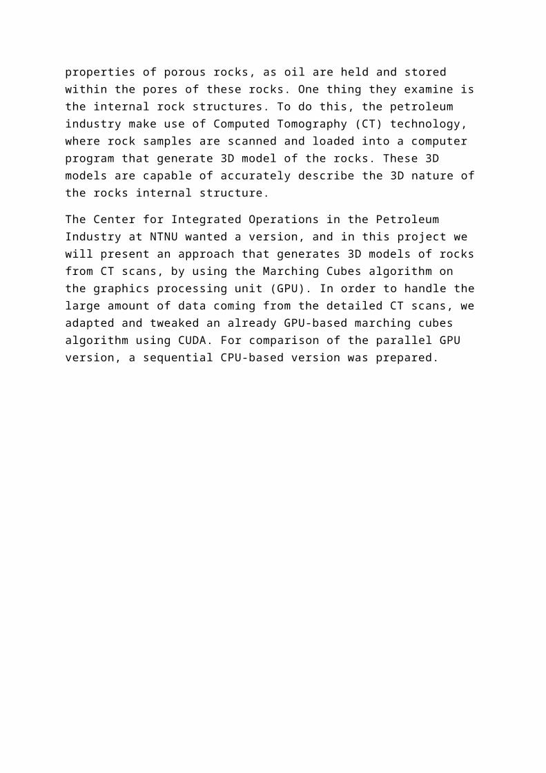
For the petroleum industry it is important to understand as much as possible about conditions that affect oil production. To get a better understanding they analyze properties of porous rocks, as oil are held and stored within the pores of these rocks. One thing they examine is the internal rock structures. To do this, the petroleum industry make use of Computed Tomography (CT) technology, where rock samples are scanned and loaded into a computer program that generate 3D model of the rocks. These 3D models are capable of accurately describe the 3D nature of the rocks internal structure.

The Center for Integrated Operations in the Petroleum Industry at NTNU wanted a version, and in this project we will present an approach that generates 3D models of rocks from CT scans, by using the Marching Cubes algorithm on the graphics processing unit (GPU). In order to handle the large amount of data coming from the detailed CT scans, we adapted and tweaked an already GPU-based marching cubes algorithm using CUDA. For comparison of the parallel GPU version, a sequential CPU-based version was prepared.

Acknowledgement

This report is the result of the work done in the course TDT4595 - Complex Computer Systems, Specialization Course. The work has been carried out at the Department of Computer and Information Science in collaboration with the Center for Integrated Operations in the Petroleum Industry, at the Norwegian University of Science and Technology.

This project and report would not have been possible without the support of several people. We wish to thank Egil Tjåland at the Department of Petroleum Engineering and Applied Geophysics and the Center for Integrated Operations in the Petroleum Industry for giving us the possibility to work on this subject, which have been an outstanding experience. We wish particularly to express the gratitude to our supervisor Dr. Anne C. Elster who was incredibly helpful and offered invaluable assistance and guidance with her extensive understanding of the field. She has been a source of great inspiration, with her always encouraging attitude and generosity through providing resources needed for this project from her own income. We also wish to convey our deepest gratitude to PhD candidate Thorvald Natvig, without his technical knowledge and support this project would not have been successful. We wish to thank Shlumberger for providing us with Petrel, Ocean and hardware resources, and we wish to express our gratitude to Wolfgang Hochweller at Shlumberger for helping us obtaining Petrel and Ocean licenses. We wish to thank NVIDIA for providing several GPUs to Dr. Anne C. Elster and her HPC-lab through her membership in the NVIDIA’s professor partnership program.

Eirik Ola Aksnes and Henrik Hesland

Trondheim, Norway, January 7, 2009

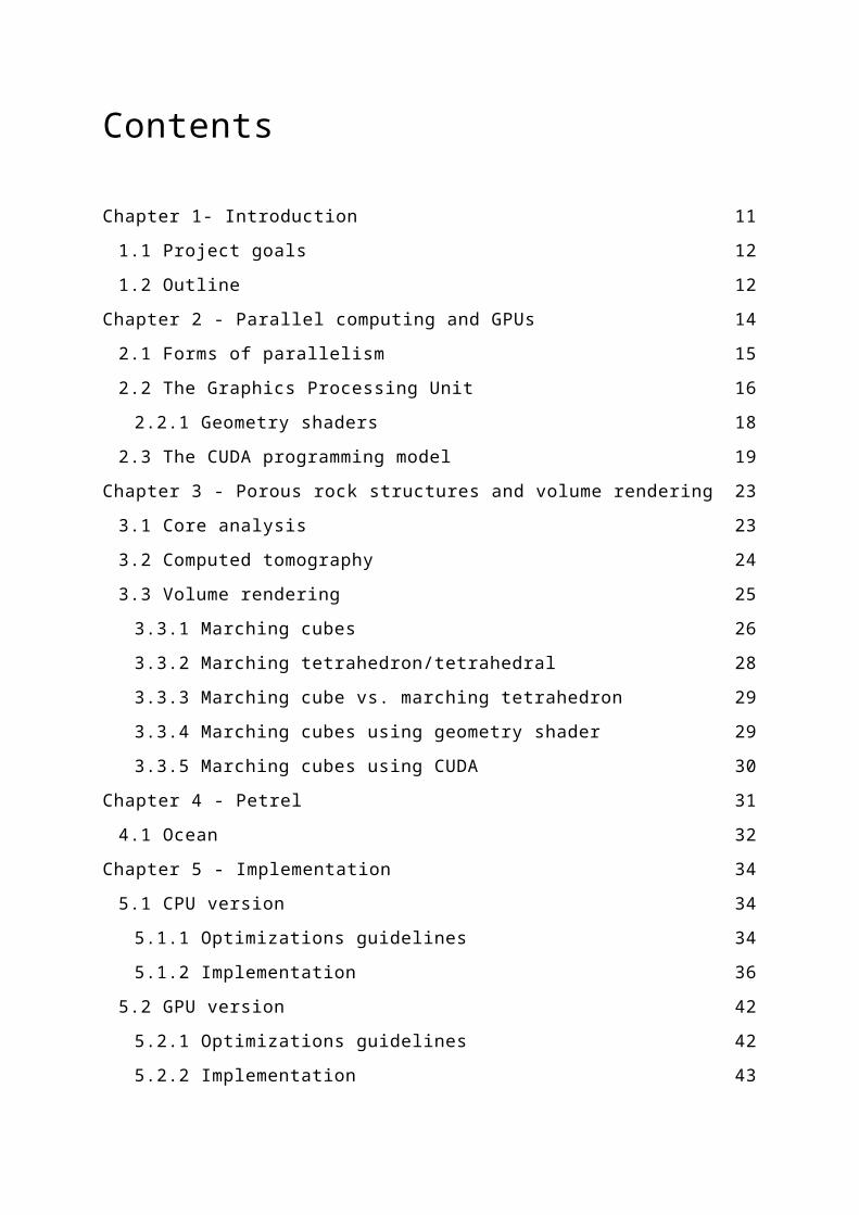
Contents

Chapter 1- Introduction 11

1.1 Project goals 12

1.2 Outline 12

Chapter 2 - Parallel computing and GPUs 14

2.1 Forms of parallelism 15

2.2 The Graphics Processing Unit 16

2.2.1 Geometry shaders 18

2.3 The CUDA programming model 19

Chapter 3 - Porous rock structures and volume rendering 23

3.1 Core analysis 23

3.2 Computed tomography 24

3.3 Volume rendering 25

3.3.1 Marching cubes 26

3.3.2 Marching tetrahedron/tetrahedral 28

3.3.3 Marching cube vs. marching tetrahedron 29

3.3.4 Marching cubes using geometry shader 29

3.3.5 Marching cubes using CUDA 30

Chapter 4 - Petrel 31

4.1 Ocean 32

Chapter 5 - Implementation 34

5.1 CPU version 34

5.1.1 Optimizations guidelines 34

5.1.2 Implementation 36

5.2 GPU version 42

5.2.1 Optimizations guidelines 42

5.2.2 Implementation 43

Chapter 6 - Benchmarks 50

6.1 GeForce 280 vs. GeForce 8800 50

6.1.1 Testing environment 50

6.1.2 Benchmarking 51

6.1.3 Discussion 52

6.2 Serial vs. parallel 52

6.2.1 Testing environment 52

6.2.2 Benchmarking 53

6.2.3 Discussion 56

6.3 Visual results 56

Chapter 7 - Conclusion and future work 61

7.1 Conclusion 61

7.2 Future work 61

List of figures

Figure 1: SPMD can select among different execution paths, SIMD cannot. Figure is from [18]. 16Figure 2: Number of floating-point operations per second for the GPU and CPU. Figure is from [8]. 16Figure 3: Memory bandwidth for the GPU and CPU. Figure is from [8]. 17Figure 4: The GPU dedicate much more transistors for data processing than the CPU. Figure is from [8]. 18Figure 5: Overview over the NVIDIA Tesla architecture. Figure is from [8]. 20Figure 6: The CUDA thread hierarchy. Figure is from [8]. 21Figure 7: The CUDA memory hierarchy. Figure is from [8]. 22Figure 8: Slice from CT scan, illustrating X-ray attenuation. 24Figure 9: A voxel with represented integer value. Figure is from [21]. 26Figure 10: The 15 cases of polygon representation. Figure is from [24]. 27Figure 11: Edge-connection-table indexing. Figure is from [21]. 27Figure 12: Dividing the dataset into tetrahedrons. Figure is from [26]. 28Figure 13: The cases of marching tetrahedral. Figure is from [28]. 29Figure 14: Shows the main modules in Petrel. 31Figure 15: The Ocean architecture. Image is from [40]. 32Figure 15: The corner indexing convention for the sequential implementation. 37Figure 16: The value of corner 3 is over the isovalue, reproduced from text [37]. 41Figure 17: Relationship between bitmaps loaded at a time and maximum numbers of vertices. 49Figure 18: Shows the runtime in seconds, in the serial vs. parallel. 54Figure 19: Shows speedup in the parallel version, relative to the serial version. 55Figure 20: Memory copying percent, 2 CT slices. 55Figure 21: Memory copying percent, 64 CT slices 55Figure 22: 20 CT slices from a reservoir rock scan. 57Figure 23: Reservoir rock, 20 CT slices. 58Figure 24: Reservoir rock, 20 CT slices. 58Figure 25: Reservoir rock, 20 CT slices. 59Figure 26: Reservoir rock, 20 CT slices. 59Figure 27: Reservoir rock, 300 CT slices. 60Figure 28: Reservoir rock, 128 CT slices. 60Figure 29: The bottom-up build process. Figure is from [32]. 63Figure 30: The element extraction in top-down traversal. Figure is from [32]. 64

List of tables

Table 1: Illustrates effective and ineffective use of cache. 35Table 2: Illustrates Loop Unrolling. 36Table 3: Shows pseudo code that describes the sequential version. 38Table 4: Shows the runtime in seconds, between the two GPUs compared. 51Table 5: Show number of vertices drawn, between the two GPUs compared. 51Table 6: Shows the runtime in seconds, in the serial vs. parallel. 53Table 7: Shows speedup in the parallel version, relative to the serial version. 54Table 8: The time usage for the most important methods in the parallel version, made with NVIDIA CUDA Visual profiler. 55

Chapter 1- Introduction

Today, 3D graphic accelerators are available for the mass marked as low-cost off-the-shelf products, as a substitute of prior expensive specialized graphics systems. A graphics processing unit (GPU) is a dedicated processor for rendering computer graphics. More or less every new computer gets shipped with a GPU, with a diverse range of capacity. As the GPU is designed for rendering computer graphics, most of the development in programming models and APIs (application programming interfaces) has been targeted at graphics applications for game consoles, personal computers and workstations. Over the last 40 years the GPU has undergone changes in its functionality and capability, driven primarily as a result of an ever increasing demand for more realistic graphics in computer games. The modern GPU has evolved from a fixed processor only capable of doing restricted graphics rendering, into a powerful programmable processor. Compared with an up to date central processing unit (CPU), the GPU utilizes a larger portion of its transistors for arithmetic and has higher memory bandwidth. The GPU has huge performances capability, which can be used to accelerate compute-intensive problems. Both CPUs and GPUs relay nowadays on architectural improvement through parallelism, which often enables a larger problem or more precise solution to be found within a practical time [17]. Parallelism also makes programming more difficult, as several parameters must be taken into consideration. Improvements in programming models and programming tools have therefore been important in the development of the GPU which allows efficient implementations and programming productivity. With the high performance capability and recent development in programmability, attention has focused on applying computationally demanding non-graphics tasks to the GPU as a high-end computational resource [10].

General-Purpose computation on GPUs (GPGPU) refers to the use of GPUs for performing computation in applications that are traditionally handled by the CPUs, for more than just graphics rendering. Since GPUs is first and foremost made for graphics rendering, it is naturally that the first attempts of programming GPUs for non-graphics where through graphics APIs. Making it tougher as programmers must master the graphics APIs and languages. To simplify this programming task and to hide the graphics API overhead, several programming models have been created. The latest release from the leading GPU supplier NVIDIA is CUDA (Compute Unified

Device Architecture), initial released in 15 th February 2007. In CUDA programmers do not need to think in terms of graphics API for developing applications to run on the GPU. It reveals the hardware functions of the GPUs directly, giving the programmer better control. CUDA is a programming model that focuses on low learning curve for developing applications that are scalable with the increase number of processor cores. It is based on a small extension to the C programming language, making it easier to get started with for developers that are familiar with the language. There are millions of CUDA enabled devices, making it feasible to accelerate applications for a broad range of people.

Several researchers have demonstrated several orders of magnitude speedup by implementing tasks to be executed on the GPU, such as n-body simulation [4], molecular dynamics [5], and weather prediction [6].

1.1 Project goals

The main objective in this project is to investigate the use of the graphics processing unit (GPU) for 3D visualization of internal pore structures of microcomputer tomography scanned rocks. The focus is on visualizing large data sets generated from detailed scans.

For the oil industry it is important to analyze properties of rocks, to achieve a better understanding of conditions that affect oil production [1]. With the use of nondestructive microcomputer tomography it is possible to make highly digital 3D representations of the internal pore structure of rocks. For useful digital representations detailed scans are needed, producing large volumetric data sets. Combined with real time requirements for fast analysis and estimations of rock properties, there is an ever increasing demand for processing power.

In this project we have chosen to look at the Marching Cubes algorithm, which are capable of building up 3D models from volumetric data sets. The GPU is a naturally choice for the visualization part of the algorithm. However, instead of letting the CPU do all the numerical calculations with building up the 3D models as ordinary, it can be useful to offload portion or all of the processing that needs to be done to the GPU for further acceleration.

1.2 Outline

The report is structured in the following manner:

Chapter 2 - Parallel computing and GPUs , describe the background information and theory as a foundation for this report.

In this chapter we will enlighten a number of benefits with parallel computing and explain different forms of doing parallelism. We will explain the modern GPUs, what tasks they are suited for and try to motivate for why one should use GPUs instead of CPUs for some computationally intensive tasks.

Chapter 3 - Porous rock structures and volume rendering, describe the background information and theory as a foundation for this report.

In this chapter we will give a brief description of reservoir rocks and core analysis. We will explain computed tomography technology, and try to motivate for why one should use this type of technology for core analysis instead of the traditional method. Volume visualization methods and techniques used for real time rendering of such porous rock structures are described.

Chapter 3 – Implementation, describe how the Marching Cubes algorithm described in Chapter 3 has been implemented.

We will in this chapter describe two different implementations of the Marching Cubes algorithm, a CPU and GPU version. We will be presented optimization guidelines for both.

Chapter 4 - Benchmarks, describes benchmarks of our implementations and discusses the results.

We will in this chapter consider the performance of our two Marching Cubes implementations. First, we will compare and evaluate the difference in running the parallel version on two different GPUs. Next, we will compare and evaluate the serial version against the parallel version. Finally, visual results of internal rock structures are shown.

Chapter 5 – Conclusion and future work, holds the conclusion and concluding remarks, and discussion on future work.

Chapter 2 - Parallel computing and GPUs

Moore’s law says that the speed of computers would double about every two years, if you look at computers today when you look at the number of transistors that can be inexpensively placed on an integrated circuit every second year it is getting harder. Whatever the peak performance of today’s processors, there will always be some problems that require or benefits from better processor speed. As explained in [16], there is a recent renaissance in parallel computing development. Increasing clock frequency is not the primary method of improving processor performance anymore, parallelism is the future. Both modern GPUs and CPUs are concerned with the increasing power dissipation, and want to increase absolute performance but also improve efficiency through architectural improvements by means of parallelism. Parallel computing often permit a larger problem or a more precise solution of a problem to be found within a practical time.

Parallel computing is the concepts of breaking up a larger problem into smaller units of tasks that can be solved concurrently in parallel. However, problems cannot often be broken up perfectly into autonomous parts and interaction is needed among the parts, both for data transfer and synchronization. The problem to be solved affects how fruitfully a parallelization is to be. If possible there would be no interaction between the separate processes, each process requires different data and produces results from its input data without need for result from other processes. Several problems are to be found in the middle, neither fully autonomous nor synchronized [17].

There are two basic types of parallel computers, if categorized based on their memory architecture [17]:

Shared memory systems that have a single address space, which means that all processing elements can access the same global memory. It can be very hard to implement the hardware to achieve uniform memory access (UMA) by all the processors with a larger number of processors, and therefore many systems have non uniform memory access (NUMA).

Distributed memory systems that are created by connecting computers together through an interconnection network, where each computer has its own local memory that cannot be accessed by the other processors. The access time to the local memory is usually faster than access time to the non-local memory.

Distributed memory will physically scale more easily than shared memory, as its memory is scalable with increase number of processors. Multiprocessor with more processors on a single chip has emerged or multicomputer, computers interconnected to form a high performance platform. Need appropriate forms of doing parallelism, which exploits the different architectures.

2.1 Forms of parallelism

There are several forms of doing parallel computing. To frequently used are task parallelism and data parallelism.

Task parallelisms, also called multiple-instruction multiple-data (MIMD), focus on distribute separate tasks across different parallel computing nodes that operate on separate data streams in parallel. It can typically be difficult to find autonomously tasks in a program and therefore task parallelism can have limited scaling ability. The interaction between different tasks occur trough either message passing or shared memory regions. Communication through shared memory region poses the problem with maintaining memory cache coherency with increased number of cores, as most modern multicore CPUs use caches for memory latency hiding. Ordinary sequential execution of a single thread is deterministic, making it understandable. Task parallelism on the other hand, even if the program is correct is not. Task parallelism is subject to faults such as race conditions and deadlock, as correct synchronization is difficult. Those faults are difficult to identify, which can make development time overwhelming. Multicore CPUs are capable of run entirely independent threads of control, and are therefore great for task parallelism [18].

Data parallelism is a form of computation that implicitly has synchronization requirements. In a data parallel computation, the same operation is performed on different data elements concurrently. Data parallel programming is very convenient for two reasons. It is easy to program and it can scale easily to large problems. The single-instruction multiple-data (SIMD) is the simplest type of data parallelism. It operates by having the same instruction execute in parallel on different data elements concurrently. It is convenient from hardware standpoint since it gives an efficient hardware implementation, because it only needs to replicate the data path. However, it has difficulty of avoiding variable work load since it does not support efficient control flow. The SIMD models have been generalized to the single-program multiple-data (SPMD), which include some control flow. Making it possible to avoid and adjust work load if there are variable amounts of computation in different parts of a program [18], as illustrated in Figure 1.

Figure 1: SPMD can select among different execution paths, SIMD cannot. Figure is from [18].

Data parallelism is essential for the modern GPU as a parallel processor, as they are optimized to carry out the same operations on a lot of data in parallel.

2.2 The Graphics Processing Unit

The Graphics Processing Unit (GPU) is a special-purpose processor dedicated for rendering computer graphics. In the pursuit for advance computer graphics over the last 40 years, the GPU has become quite computational powerful and with very high memory bandwidth, as illustrated in Figure 2 and Figure 3 it can be even higher than a modern CPU.

Figure 2: Number of floating-point operations per second for the GPU and CPU. Figure is from [8].

Figure 3: Memory bandwidth for the GPU and CPU. Figure is from [8].

The CPU is designed to maximize the execution speed of a single thread of sequential instructions. It operates on different data types (floating-point and integers), performs random memory accesses and branching. Instruction level parallelism (ILP) allows the CPU to overlap execution of multiple instructions or even change the order in which the instructions are executed. The goal is to identify and take advantage of as much ILP as possible [9]. To increase performance the CPU uses much of its transistors to avoid memory latency with data caching, sophisticated flow control and to extract as much ILP as possible. There is a limit amount of parallelism that is possible to get out of a sequential stream of instructions, and ILP causes a super linear increase in execution unit complexity and associated power consumption without linear speedup in application performance [11].

The GPU is dedicated for rendering computer graphics, and the primitives, pixel fragments and pixels can largely be processed independently and therefore in parallel (the fragment stage is typically the most computationally demanding stage [13]). The GPU differ from the CPU in the memory access pattern, as the memory access in the GPU are very coherent, when a pixel is read or write a few cycles later the neighboring pixel will be read or write. By organizing memory intelligently and hide memory access latency by doing calculations instead, there is no need for big data caches. The GPU are designed such that the same instruction operates on collections of data and therefore only need simple flow control. The GPU dedicate much more of its transistors for data processing than the CPU, as illustrated in Figure 4.

Figure 4: The GPU dedicate much more transistors for data processing than the CPU. Figure is from [8].

The modern GPU is a mixture of programmable and fixed function units, allowing programmers to write vertex, fragment and geometry programs for more sophisticated surface shading, and lighting effects. The instruction set to the vertex and fragment programs has converged, in which all programmable units in the graphics pipeline share a single programmable hardware unit. To the unified shader architecture, where the programmable units share their time among vertex work, fragment work, and geometry work.

The GPU differentiate themselves from traditional CPU designs by prioritizing high-throughput processing of many parallel operations over the low-latency execution of a single thread. Quite often in scientific and multimedia applications there is a need to do the same operation on a lot of different data elements. GPUs support a massive number of threads running concurrently and support the single-program multiple-data (SPMD) model to be able to suspend threads to hide the latency with uneven workloads in the programs. The combination of high performance, low-cost, and programmability has made the modern GPU attractive for applications traditionally executed by the CPU, for General-Purpose computation on GPUs (GPGPU). With the unified shader architecture, enables the GPGPU programmers to target the programmable units directly, rather than split up task to different hardware units [13]. To harvest the computational capability and at the same time allow programmers to be productive, need programming models that strike the right balance between low-level access to hardware resources for performance and high-level abstraction of programming languages for productivity.

2.2.1 Geometry shaders

The GPUs graphics pipeline has in the later years gotten more programmable parts. It started with the vertex shader, where a shader program could do calculations on the

input from this part of the pipeline. Later the fragment shader arrived, where shader programs could manipulate pixel-values before they were drawn on the screen. The 3rd, and latest of the shaders for the graphics pipeline, introduced in the Shader Model (SM) 4.0 is geometry shaders, and requires a NVIDIA GeForce 8800 card or newer to be computed.

The geometry shaders can be programmed to generate new graphics primitives, such as points, lines and triangles [19, 20]. Input to the geometry shader is the primitives after they have been through the vertex shader. Typically when operating on the triangles, the geometry shader’s input will be the three vertices. For storage of the output, the geometry shader then uses a vertex buffer, or the data is sent directly further through the graphics pipeline, starting with the rasterization.

As it says in the word geometry shader, it is excellent for creating geometry. An example of a geometry creation program is using the marching cubes algorithm. This will be explained further in section 3.3.4 Marching cubes using geometry shader.

A geometry shader can be programmed in OpenGL’s GLSL, DirectX’s HLSL (High Level Shader Language) and some more languages.

2.3 The CUDA programming model

There are a few difficulties with the traditional way of doing GPGPU. With the graphics API overhead that are making unnecessary high learning curve and making it difficult to debugging. In CUDA (Compute Unified Device Architecture) programmers have direct access to the hardware for better control. A programmer does not need to use the graphics API. CUDA focuses on low learning curve for developing applications that are scalable with the increase number of processor cores.

The latest generations of NVIDIA GPUs are based on the Tesla architecture that supports the CUDA programming model. The Tesla architecture is build around a scalable array of Streaming Multiprocessors (SMs) and each SM consist of several Stream Processors (SPs), that have two special function units (SFU) for trigonometry (sine, cosine and square root), a multithreaded instruction unit, and on-chip shared memory [8], as illustrated in Figure 5.

Figure 5: Overview over the NVIDIA Tesla architecture. Figure is from [8].

To a programmer, a system in the CUDA programming model consists of a host that is a traditional CPU and one or more computes devices that are massively data-parallel coprocessors. Each device is equipped with a large number of arithmetic execution units, has its own DRAM and runs many threads in parallel. The CUDA devices support the SPMD model where all threads execute the same program although they don’t need to follow the same path of execution. In CUDA, programming is done with standard ANSI C, allowing the programmer to define data-parallel functions, called a kernel that runs in parallel on many threads [12]. Parts of programs that have little parallelism executes on the CPU, while parts that have rich parallelism executes on the GPU.

GPU threads have very little creation overhead and it is possible to switch between threads that execute with near zero cost. Key to performance in CUDA is to utilize massive multithreading, a hardware technique which run thousands of threads simultaneously to utilize the large number of cores and to overlap computation with latency [15].

Under execution threads are grouped into a three level hierarchy, as illustrated in Figure 6. Every kernel executes as a grid of thread blocks, where each thread block is an array of threads that has a unique coordinate in the kernel grid. The individual threads have a unique coordinate in the thread block. Threads within the same thread block can perform synchronizing.

Figure 6: The CUDA thread hierarchy. Figure is from [8].

All threads in CUDA can access data from diverse places during execution, as illustrated in Figure 7. Each thread has its private local memory and the architecture allows effective sharing of data between threads inside a thread block, by using the low latency shared memory. Finally, all threads have access to the same global memory. There are also two additional read-only memory spaces accessible by all threads, the texture and constant memory spaces. Those memory spaces are optimized for various memory accesses patterns [8]. The CPU can transfer memory to and from the GPUs global memory using API calls.

Figure 7: The CUDA memory hierarchy. Figure is from [8].

Each SM can execute eight thread blocks at the same time. There is however a limit on how many thread blocks a SM can process at once, one need to find the right balance between how many registers per thread, how much shared memory per thread block and the number of simultaneously active threads that are required for a given kernel [12]. When a kernel is invoked, thread blocks from the kernel grid are distributed to SM with available execution capacity. As one block terminate, new blocks are lunched on the SM [8].

Under execution threads within a thread block grouped into warps. Warps are 32 threads from continuous sections of a thread block. Even though warps are not explicit declared in CUDA, knowledge of them may improve performance. The SM executes the same instruction for every thread in a warp, so only threads that follow the same execution path can be executed in parallel. If none of the threads in a warp have the same execution path, all of them must be executed sequential [12].

Chapter 3 - Porous rock structures and volume rendering

The word petroleum, meaning rock oil, refers to the naturally occurring hydrocarbons that are found in porous rock formations beneath the surface of the earth [3]. Petroleum is the result of millions of years of heat and pressure to microscopic plants and animals. Oil does not lie in huge pools, but rather within rocks or sandy mud. A petroleum reservoir or an oil and gas reservoir is an underground accumulation of oil and gas that are held and stored within porous rock formations. The challenge is how to get the oil out. The recovery of oil involves pumping water (and sometimes other chemicals) to force the oil out and the bigger the pores of the rocks there easier it is. Not just any rock is capable of holding oil and gas. A reservoir rock is characterized by having enough porosity and permeability, meaning that it has sufficient storage capacity for oil and ability to transmit fluids. It is vital for the oil industry to analyze such petrophysical properties of reservoirs rocks, to gain improved understanding of oil production.

3.1 Core analysis

Information gained through core analysis is probably the most important basic technique available for petroleum physicists to understand more of the conditions that affect production [1]. Through core analysis the fluid characteristic of the reservoir can be determined. While traditional core analysis returns valuable data, it is more or less restricted to 2D description in form of slices, and does not directly and accurately describe the 3D nature of rocks properties [14]. With the use of microcomputed tomography geoscientist can produce high-resolution 3D representations of the internal pore structures of reservoir rocks. It is a nondestructive method to determine petrophysical properties such as porosity and permeability [1]. Properties used further as inputs into reservoir models, for numerical simulations to estimate the recovery factor.

3.2 Computed tomography

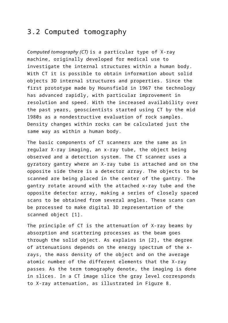
Computed tomography (CT) is a particular type of X-ray machine, originally developed for medical use to investigate the internal structures within a human body. With CT it is possible to obtain information about solid objects 3D internal structures and properties. Since the first prototype made by Hounsfield in 1967 the technology has advanced rapidly, with particular improvement in resolution and speed. With the increased availability over the past years, geoscientists started using CT by the mid 1980s as a nondestructive evaluation of rock samples. Density changes within rocks can be calculated just the same way as within a human body.

The basic components of CT scanners are the same as in regular X-ray imaging, an x-ray tube, the object being observed and a detection system. The CT scanner uses a gyratory gantry where an X-ray tube is attached and on the opposite side there is a detector array. The objects to be scanned are being placed in the center of the gantry. The gantry rotate around with the attached x-ray tube and the opposite detector array, making a series of closely spaced scans to be obtained from several angles. These scans can be processed to make digital 3D representation of the scanned object [1].

The principle of CT is the attenuation of X-ray beams by absorption and scattering processes as the beam goes through the solid object. As explains in [2], the degree of attenuations depends on the energy spectrum of the x-rays, the mass density of the object and on the average atomic number of the different elements that the X-ray passes. As the term tomography denote, the imaging is done in slices. In a CT image slice the gray level corresponds to X-ray attenuation, as illustrated in Figure 8.

z

Figure 8: Slice from CT scan, illustrating X-ray attenuation.

By use of microcomputed tomography (μCT ), much great resolution can be achieved. The machine is much smaller in construction compared to the original version used on humans, and therefore used on smaller objects. With its high resolution it is possible to distinguish density or porosity contrast within rock samples, used for detailed analysis of pore space and connectivity [1]. The highly detailed scans done by μCT producing large data sets, making it is vital to have sufficient processing power.

3.3 Volume rendering

Volume representation techniques are being used in areas from medical modeling of organs to pore-geometry for geophysicists and many other areas where deformation of 3d objects or representation of scan data is needed.

These techniques have traditionally been a serial calculation on the CPU, before it was rendered on the GPU. To generate volumes with a high level of complexity is a highly parallel task [21].

Scan data from CT or MRI is often represented as a stack of 2D images, where each image represents one slice of the volume. The volume can be computed by extracting the equal values from the scan data, and rendering them as polygonal isosurfaces or directly as a data block.

As said in [21] and [22], a volume can be completely described by a density function, where every point in the 3d-space can be represented by a single value. Each scalar-value over a threshold-value is inside the volume, while the ones under represents objects and fluids with lower density. A boundary is then placed at the threshold-values, giving the 3d model.

Marching cubes is a common algorithm for rendering as isosurfaces, and will be explained further in section

. Another way to use the same principle is the algorithm marching tetrahedron, presented further in section 3.3.2 Marching tetrahedron/tetrahedral .

To represent data with direct volume rendering, there are several methods. To mention some of them, volume ray casting, splatting, shear warp, texture-mapping and hardware accelerated volume rendering. They all require color and opacity for each sample value. If you want an overview of what each of them are see [23].

3.3.1 Marching cubes

Marching cubes is an algorithm for creating a polygonal isosurface from a 3D scalar-field. In CT and MRI scanning, each scalar represents a density value.

The algorithm, takes 8 points at a time forming a cube from a density field, then producing triangles inside of that cube, before it marches to the next cube, and repeating this until the whole scalar field is treated this way. [21]

3.3.1.1 Generation of polygons from marching cubes

The density values of the 8 corners decide how the polygons will be generated. The corners are one by one compared to a threshold value (also often called isovalue), where each corner makes a bit value representing if it is inside or outside the volume. From these bit values, it will represent an 8 bit integer, like the one in Figure 9, where corner v0, v6 and v7 are inside the volume.

Figure 9: A voxel with represented integer value. Figure is from [21].

The 8bit integer has 256 different methods the corners can be represented. Where a polygon is created by connecting together 3 points that lie somewhere on the 12 edges of the cube. With rotations of the 256 different methods, they can be reduced to 15 different cases, as illustrated in Figure 10.

Figure 10: The 15 cases of polygon representation. Figure is from [24].

If all the corner-values are either over the threshold or under it, the whole voxel is either inside or outside of the solid terrain and no polygons will be generated, like case 1 in Figure 10. And therefore there will be some empty cubes, which easily can save some computation, since they don’t need any further computation.

When a cube has at least one polygon, an interpolation computation is necessary for each vertex placed along an edge. This interpolation is calculating exactly where the density value is equal to the threshold value.

3.3.1.2 Lookup tables

Normally two lookup-tables are used, to accelerate marching cubes. The first tells how many polygons the cube will create, and the second contains an edge-connection list. Each edge in the cube has a fixed index, as illustrated in Figure 11.

Figure 11: Edge-connection-table indexing. Figure is from [21].

After a cube has calculated the 8bit integer, the algorithm will do a lookup first in the polygon-count table. The second lookup will then be done on the bit sequences that returned a number greater than 0 on the first lookup. After the second lookup, the algorithm is ready for computing the interpolation.

By rendering all the cubes’ generated polygons, the volume will be visible.

3.3.2 Marching tetrahedron/tetrahedral

Since the marching cubes algorithm was patented until June 5, 2005, other versions of the algorithm were implemented interim. One of the most important one was the marching tetrahedron [25].

The marching tetrahedron algorithm used a slightly different way to do the isosurfaces extraction than the original marching cubes algorithm. This method is some kind of way to get around the patent of the marching cubes algorithm, just with some twists. Instead of dividing the data set into cubes, this method rather divides it into tetrahedrons, where each cube is being the divided into 6 tetrahedrons by cutting diagonally through the three pairs of opposing faces, like Figure 12 [27].

Figure 12: Dividing the dataset into tetrahedrons. Figure is from [26].

A tetrahedron is a 4-corned object, and therefore there are fewer ways the vertices can be placed in it. The lookup tables will then be significantly simpler, as this algorithm leads to 16 cases to consider. With the symmetry it can even be reduced to 3 cases, where one of them either all points are inside or all outside of the volume, and there will be generated none triangles. Another case is where one point is inside and the rest outside, or the inverse there will be generated one triangle. In the last

case where 2 points are inside and the 2 others are outside, there will be generated 2 triangles making a rectangle, as you can see in Figure 13.

Figure 13: The cases of marching tetrahedral. Figure is from [28].

3.3.3 Marching cube vs. marching tetrahedron

Marching tetrahedron computes up to 19 edge-instructions pr cube, where marching cubes requires 12. Because of this, the total memory requirements are much higher, when calculating the tetrahedrons [27]. Since there are 6 tetrahedrons per cube, there is going to be 6 times more lookups than the cubes. The tetrahedrons will also produce more triangles, and therefore totally is a much more memory inefficient than the cubes. The tetrahedrons will also use 6 times more parallel threads than the cubes, where each thread is doing less computations than each thread in the marching cubes will do. Therefore, when using small datasets, which easily fits in the memory and having the same number of processors as the number of tetrahedrons in the computation, marching tetrahedron will be a better fit.

3.3.4 Marching cubes using geometry shader

With techniques such as geometry shading, we can generate volume models with acceleration from the GPU. This is a highly parallel task, and therefore a GPU, who typically has 100+ processors, is a good computation machine. Earlier the marching

cubes algorithm was programmed on vertex shader and later pixel shader for GPU acceleration of the algorithm. To program this on the GPU gave a rather hard implementation.

When the geometry shader arrived, the marching cubes algorithm could be implemented much more natural. The geometry shader lies after the vertex shader and before the rasterization stage in the graphics pipeline, as explained earlier. It will receive data in shape of primitives (points, lines, triangles) from the vertex buffer, and generate new primitives before the data is forwarded to the rasterizer.

The principle of the algorithm on this shader is that the geometry shader should receive point primitives, where each point represents a voxel/cube in the scalar field. For each point, the geometry shader will do the marching cubes lookup functions, and generate the set of triangles needed to make the isosurface. To get the scalar field values, it can be used a 16 bit floating point 3D texture, and for the table lookups for the precalculations we can use 2D textures [29].

The programming languages for programming this application can be Cg, GLSL or HLSL.

A positive matter of using the geometry shader for the acceleration of marching cubes is that it will become highly parallel, and will get high speed-up compared to a CPU-implemented version.

It is still a part of the graphics pipeline, and therefore needs to be calculated after the vertex shader. It also is limited to some primitives as input.

3.3.5 Marching cubes using CUDA

To implement the marching cubes algorithm in CUDA, it is done with a directly GPGPU approach, where a CUDA kernel is being used for all device-computations. This approach is not affected by the graphics pipeline, and therefore is more flexible than the geometry shader implementation.

Basically to make a volume from scan data, the algorithm “marches” through the voxel-field, using 8 scalar values, forming a cube in each calculation. Then making an 8 bit integer, where each corner is compared if it is inside or outside the volume. This integer is finally used to look up the cube’s vertices and polygons from a precalculated list. For a detailed description of a CUDA implementation of marching cubes, see the section 5.2 GPU version.

Chapter 4 - Petrel

Petrel is a Schlumberger owned software application for subsurface interpretation and modeling that indented to aggregate oil reservoir data from multiple sources to improve resource team productivity for better reservoir performance. It allows users to perform various workflows, from seismic interpretation to reservoir simulation. It unifies geophysics, geology, and reservoir engineering domains, reducing the need for multiple highly specialized tools. The Figure 14 shows the main modules of Petrel.

Figure 14: Shows the main modules in Petrel.

The software development of Petrel was started in Norway by a company called Technoguide in 1996. In 1998, Petrel became commercially available in 1998, and was developed specially for PC- and Windows OS- users with a familiar Windows-like user interface. The familiar interfaces lead to a fast learning curve for less experienced users, and more staff without specialist training should be able to use 3D geologic modeling tools, than earlier programs [39]. The later years, after Schlumberger acquired Technoguide in 2002, Petrel has grown significantly, and lots of other functionality, like seismic interpretation and well planning included. Petrel

has also been built on a software framework called Ocean, where 3 rd party users can develop their own modules to run in Petrel.

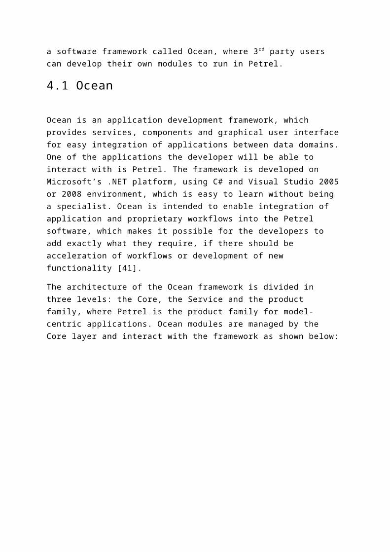
4.1 Ocean

Ocean is an application development framework, which provides services, components and graphical user interface for easy integration of applications between data domains. One of the applications the developer will be able to interact with is Petrel. The framework is developed on Microsoft’s .NET platform, using C# and Visual Studio 2005 or 2008 environment, which is easy to learn without being a specialist. Ocean is intended to enable integration of application and proprietary workflows into the Petrel software, which makes it possible for the developers to add exactly what they require, if there should be acceleration of workflows or development of new functionality [41].

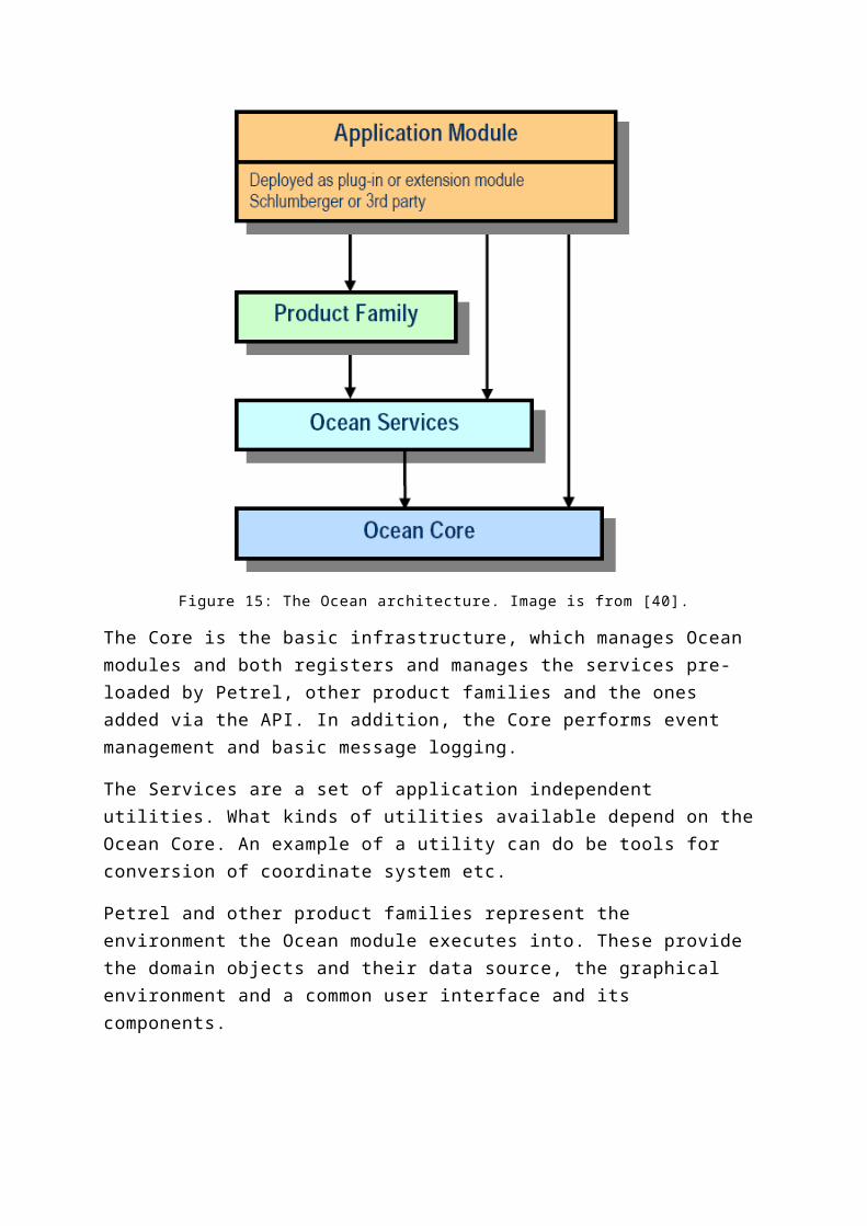
The architecture of the Ocean framework is divided in three levels: the Core, the Service and the product family, where Petrel is the product family for model-centric applications. Ocean modules are managed by the Core layer and interact with the framework as shown below:

Figure 15: The Ocean architecture. Image is from [40].

The Core is the basic infrastructure, which manages Ocean modules and both registers and manages the services pre-loaded by Petrel, other product families and the ones added via the API. In addition, the Core performs event management and basic message logging.

The Services are a set of application independent utilities. What kinds of utilities available depend on the Ocean Core. An example of a utility can do be tools for conversion of coordinate system etc.

Petrel and other product families represent the environment the Ocean module executes into. These provide the domain objects and their data source, the graphical environment and a common user interface and its components.

At last the application modules connect to the other layers of the software through the .NET framework, where the development can be done.

Further information about Ocean can be found in [40, 41].

Chapter 5 - Implementation

This chapter describes how the algorithm presented in section

, has been implemented. For this project we implemented two versions of the marching cubes algorithm. The first implementation is a serial, using the CPU. That was implemented because of need to evaluate the second version, the GPU version, which is tuned for parallelization.

For rendering both the CPU and GPU version uses Vertex Buffer Objects [36], which is an OpenGL extension that provides methods for uploading data directly to the GPU, and offer significant performance increase because data can be rendered directly from the GPU memory. Rather than have to store it into main memory and have to transfer it to the GPU each time wish to redraw a scene.

5.1 CPU version

This section describes the CPU version of the marching cube algorithm. The CPU version uses only one processor core for execution, even if the processor used have more than one processor core (multicore). Before we describe the implementation details, we will present some optimizations guidelines for maximizing the CPU performance.

5.1.1 Optimizations guidelines

In an ideal world, the modern compilers would completely handle the optimization of our program. However, the compiler has too little knowledge of our source code to be able to do so. It is possible to choose the degree of optimization that the compilers should do on our code, and one should be aware that the highest degree might lead to

slower code and not faster. So need to try the different optimization options independently. In any case, compilers often accelerate performance by selecting the right compiler options. There are also some general optimization techniques programmers should be acquainted with for highest possible performance.

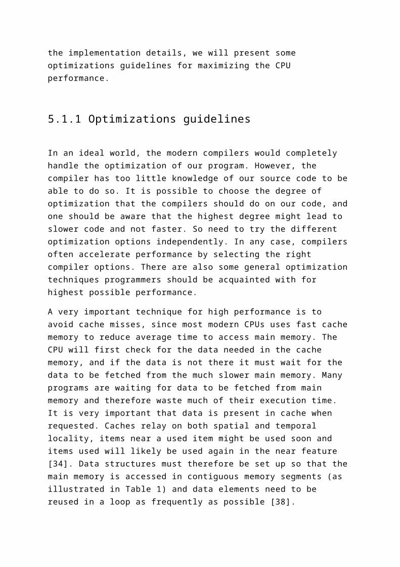
A very important technique for high performance is to avoid cache misses, since most modern CPUs uses fast cache memory to reduce average time to access main memory. The CPU will first check for the data needed in the cache memory, and if the data is not there it must wait for the data to be fetched from the much slower main memory. Many programs are waiting for data to be fetched from main memory and therefore waste much of their execution time. It is very important that data is present in cache when requested. Caches relay on both spatial and temporal locality, items near a used item might be used soon and items used will likely be used again in the near feature [34]. Data structures must therefore be set up so that the main memory is accessed in contiguous memory segments (as illustrated in Table 1) and data elements need to be reused in a loop as frequently as possible [38].

Effective use of cache Ineffective use of cache

for i=0…4 for j=0…4 a[i][j]= …

Memory are continuous:

for j=0…4 for i=0…4 a[i][j]= …

Memory are not continuous:

Table 1: Illustrates effective and ineffective use of cache .

Loop optimization techniques can have huge effect on cache performance, since most of the execution time in scientific applications is used on loops. Matrix multiplication is one example that can gain performance if the sequence of how the for loops are correctly arranged, by allowing optimal data array access pattern. If the data needed is in continuous memory, the next elements needed are more likely to be in the cache. You can improve cache locality by dividing the matrix into smaller sub matrixes, and choose optimal block size that will fit into cache and reduce execution time. The size of the sub matrix will be system depended, since different size of cache for different systems.

Another feature of today’s processor architectures is the long execution pipelines, which offers significant execution speedups if kept full. With pipelining several instructions can be overlapped in parallel. Branch predication is used to ensure that the pipeline is kept full, by guessing which way the branch is most likely to go. It has significant impact on performance, by letting processors fetch and start execute instructions without waiting for the branch to be determined. A Conditional branch is a branch instruction that can be either taken or not taken. If the processor makes the

wrong guess in a conditional branch, the pipelined needs to be flushed and all computation before the branch point is unnecessary. It can therefore be advantageous to eliminate such conditional branches in performance critical places in the code. One technique that can be used to eliminate branches and data dependencies is to unroll loops [35], as illustrated in Table 2.

Regular loop Unrolled loop

for(int i=1; i<N; i++) if((i mod 2) == 0) a[i] = x; else a[i] = y;

for(int i=1; i<N; i+=2) a[i] = y; a[i+1] = x;

Table 2: Illustrates Loop Unrolling.

Only should try to reduce the use of if-sentences as much as possible inside the inner loops.

5.1.2 Implementation

This section will describe our sequential implementation of the marching cube algorithm. The implementation and this description of it is build upon earlier applications gathered from [12, 37]. The compiler used for the implementation was Microsoft Visual C++, in the operating system Microsoft Windows Vista 32bit. The program has been programmed in C and C++. The graphics library used is OpenGL 1, with the use of the OpenGL Extension Wrangler Library (GLEW) 2 for access to Vertex Object Buffers, enabling effective rendering. For window management and handling mouse and keyboard user inputs, the Simple DirectMedia Layer (SDL) 3 is used. SDL is a cross-platform library for access to low level access to audio, mouse, keyboard and OpenGL and the frame buffer. To load BMP files, the EasyBMP 4 library is used. EasyBMP is a simple cross-platform, open source C++ library.

Microcomputed Tomography scans generating large data sets, making it extremely important that the memory usage is optimal. That permits the maximum quantity of data to be used at same time, without running out of memory. All data structures used in the sequential version uses and store only the minimum of what is required to generate the volumetric models of the reservoir rocks.

1 http://www.opengl.org/2 http://glew.sourceforge.net/3 http://www.libsdl.org/4 http://easybmp.sourceforge.net/

The sequential algorithm takes 8 points at a time forming a cube that has the following corner indexing convention:

Figure 16: The corner indexing convention for the sequential implementation.

The algorithm uses two lookup tables, as explained in section 3.3.1.2 Lookup tables.

The pseudo code for the sequential implementation

Create the edge and triangle lookup tables

Allocate memory for each triangle that will be generated

Allocate memory for edge intersection points

for z = 0...size_z-1 for y = 0...size_y-1 for x = 0…size_x-1 (1) Find out where in the edge table we should do lookup, by creating an 8 bit index (2) If not all points are on the inside or outside, want to take a closer look (2.1) Find out by doing a lookup into the edge table, where along each cube edge, the isosurface crosses and do linear interpolation to find the intersection points (2.2) Lookup and loop through entries in the triangle lookup table to decide which of the edge intersections points found in (2.1), to draw triangles between

Table 3: Shows pseudo code that describes the sequential version.

Additional explanation to the pseudo code described above, where we also presents some sections from the implemented source code:

(1) Find out where in the edge table we should do lookup, by creating an 8 bit index

An 8 bit index is formed by using the |= operator, where each bit match up to a corner in the cube, as illustrated under. See section 3.3.1.1 Generation of polygons from marching cubes, for further explanation.

V7 V6 V5 V4 V3 V2 V1 V0

The bitwise OR assignment operator (|=) looks at the binary representation of the value of the result and expression and does a bitwise OR operation on them. The result of the OR operator behaves like this [34]:

Operand1 Operand2 Operand1 OR Operand20 0 00 1 11 0 11 1 1

Listed under is connection between each cube corner, and its binary and decimal number representation used to determine the 8 bit index:

Corner Binary Decimal V0 1 1V1 10 2V2 100 4V3 1000 8V4 10000 16V5 100000 32V6 1000000 64V7 10000000 128

Section from the implemented source code, where we find out where in the edge table we should do lookup:

// vertex 0if(this->rock->SgVolume(x, (y+1), (z+1)) > this->iso_value) lookup |= 1; // vertex 1if(this->rock->SgVolume((x+1), (y+1), (z+1)) > this->iso_value) lookup |= 2; // vertex 2 if(this->rock->SgVolume((x+1), (y+1), z) > this->iso_value) lookup |= 4;// vertex 3if(this->rock->SgVolume(x, (y+1), z) > this->iso_value) lookup |= 8;

// vertex 4if(this->rock->SgVolume(x, y, (z+1)) > this->iso_value) lookup |= 16; // vertex 5if(this->rock->SgVolume((x+1), y, (z+1)) > this->iso_value ) lookup |= 32; // vertex 6if(this->rock->SgVolume((x+1), y, z) > this->iso_value) lookup |= 64; // vertex 7if(this->rock->SgVolume(x, y, z) > this->iso_value) lookup |= 128;

(2) If not all points are on the inside or outside, want to take a closer look

Section from the implemented source code, where we are not interested in a closer look if the lookup value is 0 or 255, since then the cube does not contribute to the isosurface.

if ((lookup != 0) && (lookup != 255))

(2.1) Find out by doing a lookup into the edge table, where along each cube edge, the isosurface crosses and do linear interpolation to find the intersection points

Looking up in the edge table by using the index found in (1) returns a 12 bit number representing which edges that are crossed, this number are used with & operator. This will be used to find out if one edge are crossed by the isosurface, if it does it needs to be interpolated. All interpolated points are put in an array for further use in (2.2).

Under is listed a section from the implemented source code that is used to find out if the edge between 0-1 and 1-2 are crossed by the isosurface. That is also done between the edges 2-3, 3-0, 4-5, 5-6, 6-7, 7-4, 0-4, 1-5, 2-6 and 3-7.

if (this->edgeTable[lookup] & 1) // 0 - 1{

vertex v0((float) x,(float) (y+1),(float) (z+1)); v0.flux = this->rock->SgVolume(v0.x_pos, v0.y_pos, v0.z_pos);vertex v1((float) (x+1),(float) (y+1),(float) (z+1));v1.flux = this->rock->SgVolume(v1.x_pos, v1.y_pos, v1.z_pos);this->verts[0] = this->rock->interpolate(v0, v1); // interpolate edge 0 to 1

}if (this->edgeTable[lookup] & 2) // 1 - 2{

vertex v1((float) (x+1),(float) (y+1),(float) (z+1));v1.flux = this->rock->SgVolume(v1.x_pos, v1.y_pos, v1.z_pos);vertex v2((float) (x+1),(float) (y+1),(float) z);v2.flux = this->rock->SgVolume(v2.x_pos, v2.y_pos, v2.z_pos);this->verts[1] = this->rock->interpolate(v1, v2); // interpolate edge 1 to 2

}

The source code for the linear interpolations is:

inline vertex interpolate(vertex v1, vertex v2){

vertex v; float diff;

diff = (this->iso_value - v1.flux) / (v2.flux - v1.flux);

v.x_pos = v1.x_pos + diff * (v2.x_pos - v1.x_pos);v.y_pos = v1.y_pos + diff * (v2.y_pos - v1.y_pos);v.z_pos = v1.z_pos + diff * (v2.z_pos - v1.z_pos);

return v;}

(2.2) Lookup and loop through entries in the triangle lookup table to decide which of the edge intersections points found in (2.1), to draw triangles between

Under is listed a section from the implemented source code where the edge intersection points found in (2.1) are used to put together one or up to 5 triangles for the isosurfaces. By doing a lookup into the triangle table with the same index found in (1), we find out which of the intersections points to drawn triangles between. Every triangles normal is determined, and stored with its corresponding triangle for further rendering.

for (i = 0; this->triTable[lookup][i] != -1; i+=3){

vertex v1 = this->verts[this->triTable[lookup][i]];vertex v2 = this->verts[this->triTable[lookup][i+1]];vertex v3 = this->verts[this->triTable[lookup][i+2]];

vertex n = CalcNormal(v1,v2,v3);

d_pos[v_gen] = make_float4(v1.x_pos,v1.y_pos,v1.z_pos,1.0f);d_normal[v_gen] = make_float4(n.x_pos,n.y_pos,n.z_pos,1.0f);d_pos[v_gen+1] = make_float4(v2.x_pos,v2.y_pos,v2.z_pos,1.0f);d_normal[v_gen+1] = make_float4(n.x_pos,n.y_pos,n.z_pos,1.0f);d_pos[v_gen+2] = make_float4(v3.x_pos,v3.y_pos,v3.z_pos,1.0f);d_normal[v_gen+2] = make_float4(n.x_pos,n.y_pos,n.z_pos,1.0f);

v_gen += 3;}

In Figure 17, an illustration that summarizes how our sequential Marching Cubes works is presented, where the value of the corner 3 is over the isovalue.

Figure 17: The value of corner 3 is over the isovalue, reproduced from text [37].

5.2 GPU version

First we will explain some optimization guidelines for CUDA, then an explanation of the GPU implementation.

5.2.1 Optimizations guidelines

To program efficiently on a GPU using CUDA, the knowledge of the hardware-architecture is important. That is explained further in the section 2.3 The CUDA programming model.

The primary performance element of the GPU, which really should be exploited by a CUDA programmer, is the large number of computation cores. To do this, there should be implemented a massive multithreaded program.

One of the problems with a GPU implementation is the communication latency. For computations, there should be as little communication as possible between the CPU and GPU, and often some time can be spared by doing the same computation several times, than load the answers between the CPU and GPU. The massive parallelization of threads is also important for hiding the latency.

A modern GPU contains several types of memory, where the latency of these is different. To reduce the used bandwidth, it is recommended to use the shared memory where it is possible. The global device memory is divided into banks, where access to the same bank only can be done serially, but access to different banks can be done in parallel. Therefore the threads should be grouped to avoid this memory conflict.

Another function that should be used as little as possible is synchronization. This can cause many threads to wait a long time for another thread to finish up, and can slow the computation significantly.

When using strategies to reduce the number of computations in an implementation, a restriction to another element of the GPU could often be met. Therefore the number of threads, memory used and total bandwidth should be configured carefully in proportion to each other.

The number of thread-blocks used simultaneously on a streaming multiprocessor (SM) is restricted by the number of registers, shared memory, maximum number of active threads per SM and number of thread-blocks pr SM at a time.

5.2.2 Implementation

The compiler used for the implementation was Microsoft Visual Studio 2005 in the operating system Microsoft Windows Vista 32bit. This implementation is build upon NVIDIA’s marching cubes example from CUDA beta 2.1 SDK. Most of the program has been programmed in CUDA C and C99, with a little hint of C++ for easier array-lookup.

The GPU implementation contains the following files:

tables.h: The marching cubes precalculated tables. cudpp.h: C++ link-file for CUDPP library. marchingCubes_kernel.cu: Device kernel. marchingCubes.cpp: Host control.

The files will now be explained further.

5.2.2.1 The marching cubes precalculated tables: table.h

This file contains two tables for fast lookup. The tables have the needed recalculated values for the marching cubes algorithm to be accelerated. Both of these tables use the cube index as reference for the lookup.

The first table is the triangle table. In this table, there are 256 different entries, which each having a list of 3 and 3 edges that together makes a triangle. The maximum number of triangle a cube can produce is 5, and therefore each entry contains a list with 15 edge indices.

The last one is a vertex count table. A lookup on this table will return the number of vertices the current cube index should generate. And this will both decide how much memory to allocate and how many times to loop the triangle generation-loop for the current cube.

5.2.2.2 C++ link-file for cudpp library: cudpp.h

Cudpp.h is a simple file, who calls functions from the CUDPP library. This file is basically made for communication between C++ files and the library.

CUDPP (CUDA Data Parallel Primitives) Library is a library of data-parallel algorithm primitives such as parallel scan, sort and reduction. The library focuses on performance, where NVIDIA says that they aim to provide the best-of-class

performance for their primitives. Another important aspect of the library is that it should be easy to use in other applications.

In our application, we are using the scan (prefix sum) function to perform stream compaction. This is where we scan an array holding the number of vertices to be generated pr voxel, and returning an array holding the vertices number each voxel should start with when saving the data to the vertex buffer objects.

5.2.2.3 Device kernel: marchingCubes_kernel.cu

The file marchingCubes_kernel.cu contains all computations on the device. Most of the functions found here are the ones best fitted for parallelization. The other ones are support functions for preparing the algorithm and some for doing parts of the calculations.

In the first of the support categories, we have the function allocateTextures. This function is copying the precalculated lookup-tables to the texture cache, for fast lookups.

All the parallel functions have parameters for both grid and number of threads. These numbers decides the size of the parallelization, where the thread number means how many threads there should be calculated pr threadblock.

The main functions will be explained further:

5.2.2.3.1 classifyVoxel

This is where each voxel will be classified, based on the number of vertices it will generate. It first gets the voxel by calculating the threads grid position and grabs the sample points (one voxel pr thread). Then when the calculation of the cube index is done, the texture lookup is launched and the vertices count for the current voxel is saved in an array on the global memory.

5.2.2.3.2 compressVolume

Since the datasets we are operating on contains so much data, we decided to compress the dataset to 1/8 th the size before calculating the marching cubes algorithm. This was because the number of vertices generated from the raw dataset was about 5-8 times too many to draw for the best graphics card available to us at

that moment, the NVIDIA GeForce 280 GTX card. The function compressVolume is doing the compression and making the scalar-field-data 1/8 of the original size.

5.2.2.3.3 addVolume

This function should discard the frames around each image from the dataset, and therefore save some memory. Most of the frames are 25-40 pixels wide along the edges. With the 1000*1000 bmp images we used for testing, this could save us up to 153600 8 bit uchar values pr image, and could therefore be vital for our algorithm.

But since different data-sets have different layouts, we decided to comment out the frame removal for the final version, and the function addVolume is now a simple one, copying the image densities to the device.

5.2.2.3.4 generateTriangles2

To generate the triangles after the volume has been classified, it is needed to make a lookup in another table than classifyVoxel does. Since throughput is the GPU’s biggest strength and latency is a slow matter, we decided to keep NVIDIA’s way to do this algorithm. The algorithm is basically doing what classifyVolume did at first, where it finds the grid position, collects the sample data and calculates the cube index. Here we also calculate the position in the 3 dimensional world for each of the eight corners of the current cube. After this it makes an interpolation-table for each edge, which calculates where on the current edge the isovalue might be. Finally the function loops through all of the triangles to be generated for the current cube, and calculates its vertices coordinate-position and normal vectors.

5.2.2.4 Host control: marchingCubes.cpp

The file marchingCubes.cpp is the main file in the system. We have implemented two versions of this file. One of them is for the standalone application using OpenGL to show the algorithm. The other version is prepared for ocean-implementation. First we will explain the main functions existing in both of the versions, then explain the difference in the implementation.

5.2.2.4.1 calcBitmaps

This function is quite simple, where the path for the directory for the scan data are being evaluated and determined how many bmp-images the algorithm is going to load. The quantity of bitmaps in the directory symbolizes the step size in the z-direction of the final volume.

5.2.2.4.2 calcBitSize

Another help-function for loading the scan data is calcBitSize. In this file, the width and height of each image is decided. These values correspond to the step size in the x and y directions of the volume. Another value who is determined in this function is the number of colors in a bitmap. Since 8bit bmp files contain a palette, who is a lookup table for the colors in the image, this one has to be decided to extract the colors. The scan data we tested with had a 256 grayscale colored palette, and each of the lookup indices represented the same grayscale-color, and therefore this value is saved for easier use of other datasets.

5.2.2.4.3 loadBMPFiles

This function is the bitmap loader, where a parameter decides how many pictures to load at a time. The function is loading one and one image, copying it to the device, and then calling the device function addVolume. addVolume will then remove the unwanted parts of the picture, and make the density volume ready for further calculations

5.2.2.4.4 initMC

initMC is the function that controlls everything with the calculation of the volume. It first initiates all the values for the algorithm, where the values for maximum number of vertices and number of loaded pictures at a time decides how the devices global memory is being used. The more vertices wanted to be drawn in the final volume model, the fewer bitmaps can be calculated at one time, and the throughput is lesser exploided. Therefore it is important to adjust these values in propotion to the current device and data set that is being used. For more information about this, look at 3.1.7.

Given how many bitmaps to load at a time, the function will further loop through the dataset, using loadBMPFiles, classifyVoxel, cudppScan and generateTriangles2. For each time this loops, the generated triangles and their normal vectors will be saved in two vertex buffer objects (VBOs). The VBO is easy and fast to draw with few lines of OpenGL code and will be the important link between the Ocean and CUDA-files.

5.2.2.5 Standalone version

In addition to the function the two version share, the standalone version contains function for drawing and storing the volume. For the storing is, as explained in 3.1.4.4, VBOs used. There are some standard OpenGL functions, opening a window and setting the light adjustments. In addition there are implemented functions for keyboard input and for the mouse to spin the volume. The function renderIsosurface is then drawing the VBOs each frame.

5.2.2.6 Schlumberger Ocean prepared version

In the Schlumberger Ocean prepared version most of the OpenGL, like open window and key handlers are removed. The only thing left from the OpenGL libraries is the creation and removal of the VBOs. The two VBOs contain all information needed to draw the volume, and therefore device addresses to the locations where these is saved, is the only information Ocean is getting back from the function call. The function Ocean calls is the main function in marchingCubes.cpp, and its needed parameters is the path of the storage location for the data set to generate volume from, the isovalue, the maximum number of vertices to be generated and the number of bitmaps to load at a time. With this information an Ocean implementation of our program can be easily implemented.

5.2.2.7 Memory allocation

Our program is very memory dependant, and to control the memory, you have to know how much memory the device contains. There are created two variables to control the memory allocation. The first of these variables are maxVerts, which control how many vertices the device should maximally be able to draw. And the second variable is bitmapsPrTime, where the digit represents the number of bitmaps to load to the device memory at a time.

The variable maxVerts are controlling the size to allocate for the two device-lists posVBO and normalVBO. Each entry in each of these lists contains 4 float values, and will therefore use the allocated memory size 4*4 bytes (size of float) = 16 bytes (pr entry in each list). The other variable controls the device-lists d_volume, d_voxelVerts and d_voxelVertsScan. The size of d_volume, who contains the raw density volume as unsigned character values, is pixelsPrBitmap*bitmapsPrTime*1 byte, and the size of the two other lists is for each double the size of d_volume, since

they contains unsigned integers for storing values. These two voxel vertice-lists are for storing the computed data from the functions classifyVolume and the scan-data for the CUDPP-scan.

The big datasets we were doing the tests with all contains bitmaps with 1000x1000 pixels, where most of them were drawing between 10 000 000 and 16 000 000 vertices, when we compressed the volume to 1/8 th the total size, meaning halving the bitmaps to 500x500 pixels. When loading bitmaps, we use memory to temporary save in a list, before compressing the data and the lists d_voxelVerts and d_voxelVertsScan is allocated on the device after the bmp load is finished. Therefore the functions then for storing the data would look like this:

While loading the bitmaps:

spaceAllocated=( maxVerts×16bytes × 2lists )+(bitmapsPrTime× (500 ×500 ) pixelsbitmap

×1byte)+(4 × (500× 500 ) pixelsbitmap

× ( (bitmapsPrTime∗2 )+1 ))

While computing the CUDA marching cubes:

spaceAllocated=( maxVerts×16bytes × 2lists )+(bitmapsPrTime× (500 ×500 ) pixelsbitmap

×5bytes)The loading of bitmaps will take the most memory of these two. If we do not use the image compression algorithm, we do not use the big temporary list when loading bitmaps, in this case the one while computing the CUDA functions will use the most memory, but it will change a little, cause of the original width and height of each image is used:

While computing the CUDA marching cubes:

spaceAllocated=( maxVerts×16bytes × 2lists )+(bitmapsPrTime× (1000 ×1000 ) pixelsbitmap

×5 byte)For testing the datasets we were using the NVIDIA GeForce 280 GTX with 1GB device memory. For different datasets this will lead to this allocation conditions:

1000

0000

1100

0000

12000

000

1300

0000

14000

000

1500

0000

1600

0000

17000

000

0

50

100

150

200

250

300

350

400

With bmp compressionWithout bmp compress

Figure 18: Relationship between bitmaps loaded at a time and maximum numbers of vertices.

The precalculated lists are allocated on the device memory, but totally they take 8.5 kb, and therefore are not taken in our computation. There are also used some other integer values in addition to some memory used for the OpenGL functionality for buffers and lights that is not used in these computations. This are because our computations shows the roof of the relationship between the numbers of bitmaps loaded at a time and the maximum number of vertices to draw on a GPU with 1GB global device memory.

On Figure 18, we can observe that with the bmp compression, we can load about twice as many bitmaps at a time, compared to the one without the compression. The vertice-count when using the compression is also about 1/8 th compared to use the raw data to compute the vertices. When not using the compression, the vertice count, and therefore the memory needed are much greater.

An average data-set we used for testing required around 12 000 000 vertices with the compression algorithm in use, and therefore we could see that we the number of bitmaps to load at a time is about 300.

Chapter 6 - Benchmarks

In this chapter, we will consider the performance of our implementations described in the previous chapters. For the evaluation of our algorithm, we ran two types of tests, the first where we compare the performance when running the parallel version on two different GPUs. The second test is a speedup calculation between the serial marching cubes algorithm and the parallel one for the GPU.

6.1 GeForce 280 vs. GeForce 8800

In this section we will compare the performance of our parallel implementation of the Marching Cubes algorithm, by running it on two different GPUs.

6.1.1 Testing environment

The first GPUs enabled for Shader Model 4.0 and therefore also CUDA was the NVIDIA GeForce 8800, where the GTX was the high-end version and GTS the more economic one. The 8800-card was released November 8 th, 2006 [30]. At the time we were doing the benchmark-tests, NVIDIA’s GeForce 280 GTX, who was released June 17th, 2008 [31], was the best CUDA enabled card with graphics output on the marked. Therefore the parallel version of the program is compared between these two, to see how much the computation power has changed in these 18 months for our implementation. The test-machines were having these specifications:

Machine 1:

CPU Intel® Core™ 2 Quad CPU Q9550, 2.83 GHz, and 12 MB L2 Advance

Smart Cache.

Memory OCZ DDR3 4GB Platinum EB XTC Dual Channel

GPU NVIDIA GeForce GTX 280

GPU Engine Specs: 240 Processor Cores, 602 MHz Graphics Clock, and

1296 MHz Processor Clock.

Memory Specs: Memory Clock 1107 MHz, 1 GB DDR3 SDRAM, and

Memory Bandwidth 141 GB/sec.

Memory

setup

Number of bitmaps at a time: 70

Maximum vertices: 16 000 000

Machine 2:

CPU Intel® Core™ 2 Duo CPU E6600, 2.4 GHz.

Memory Corsair TWIN2X 6400 DDR2, 2GB CL5

GPU Asus GeForce 8800 GTS

GPU Engine Specs: 96 Processor Cores, 1200 MHz Processor Clock.

Memory Specs: 640 MB DDR3 SDRAM, and Memory Bandwidth 64

GB/sec.

Memory

setup

Number of bitmaps at a time: 40

Maximum vertices: 11 000 000

6.1.2 Benchmarking

Runtime of the two GPUs compared in seconds:

GPU N 10002 25 10002 301 10002 5701 - GTX 280 0.0535 0.3005 0.57842 - 8800 GTS 0.1926 1.0415 2.0322Speedup GTX280 3.60 3.47 3.51

Table 4: Shows the runtime in seconds, between the two GPUs compared.

Vertices drawn:

GPU N 10002 25 10002 301 10002 570

1 - GTX 280 1 314 426 11 849 466

11 681 184

2 - 8800 GTS 1 314 426 11 000 000

11 000 000

Table 5: Show number of vertices drawn, between the two GPUs compared.

6.1.3 Discussion

The test-machines have some big differences in both computation power and memory. Where the 280 card can load about double of what the 8800 card can at a time, making the 280 card to be able to load more bitmaps at a time. The more times the main loop is looping, the more bitmaps will be loaded two times, since the last bitmap in one round will be loaded first in the next round. But the loading of images is not taken into consideration of the timer.

The 280 card has 30 streaming multiprocessors (SMs) versus 12 on the 8800 card. This leads to about three times higher amount of computations available to be done per clock cycle.

Another big difference between the two GPUs is the global memory bandwidth. Where the 280 card has 141.7 GB/s versus 8800’s 64 GB/s, which will make the memory operations on the 280 over twice as fast as the 8800’s.

Since the marching cubes algorithm contains a massively parallel amount of computations, where each computation uses both lookups and storing on the global memory, both the number of SMs and the bandwidth is large factors for the 280 card’s speedup. The memory of the 8800 card will make restrictions between if it could draw all the wanted vertices and how many bitmaps to be loaded at a time. We can also observe from the results that the speedup is about the same independent of the dataset size. These speedup-factors is then mostly affected by the amounts of computations to be performed simultaneously and the global bandwidth.

6.2 Serial vs. parallel

In this section we will compare our serial and parallel implementation of the Marching Cubes algorithm.

6.2.1 Testing environment

The tests were run in the operating system Microsoft Windows Vista 32-bit. We ran only 32-bit computations, since 32-bit of precision is most common to the CPU and GPU. The system was completely unused when the tests were run. For visual profile generation of memory and processing in the parallel version, we used the NVIDIA CUDA Visual profiler (version 1.1.6). All the different programs were compiled with Microsoft Visual C++, using Microsoft Visual Studio 2005. With the following

compile time optimization options tested: Disabled (/Od), minimize size (/O1), maximize speed (/O2), full optimization (/Ox) and whole program optimization (/GL).

We ran the performance tests on the following machine:

CPU Intel® Core™ 2 Quad CPU Q9550, 2.83 GHz, and 12 MB L2 Advance

Smart Cache.

Memory OCZ DDR3 4GB Platinum EB XTC Dual Channel

GPU NVIDIA GeForce GTX 280

GPU Engine Specs: 240 Processor Cores, 602 MHz Graphics Clock,

and 1296 MHz Processor Clock.

Memory Specs: Memory Clock 1107 MHz, 1 GB DDR3 SDRAM, and

Memory Bandwidth 141 GB/sec.

6.2.2 Benchmarking

All the tests were run with the same data (from the same CT scan) and with identical isovalue, for best possible evaluation.

The following two programs were tested:

CPU Q9550 - The CPU version, with the /Ox and /GL compile time optimization options enabled for maximum performance.

GPU GTX 280 - The GPU version.

Runtime in seconds of the two programs:

Program N 10002 2 10002 4 10002 8 10002 16 10002 32 10002 64

GPU GTX 280 0.0067 0.0118 0.0228 0.0544 0.0778 0.1565

CPU Q9550 0.0405 0.1206 0.2786 0.5764 1.1863 2.4606Table 6: Shows the runtime in seconds, in the serial vs. parallel.

2 4 8 16 32 640

0.5

1

1.5

2

2.5

3

GPU GTX 280CPU Q9550

Number of CT slices

Runti

me

in se

cond

s

Figure 19: Shows the runtime in seconds, in the serial vs. parallel.

The commonly metric used for measuring the parallel performance is the speedup. The speedup factor S( p) is a measure of relative performance, given by:

S ( p )=t s

t p

Where t s is the execution time of the best sequential algorithm running on a single processor and t p is the execution time for solving the same problem on a multiprocessor. The maximum speedup possible is p with p processors, called linear speedup, given by:

S ( p )≤

t s

t p

p=p

However, this is not often achieved because of additional overhead in the parallel version. Inactive processors, additional computation and communication time between processes are often factors that will limit the possible speedup in the parallel version [17].

Speedup in the parallel program:

Program N 10002 2 10002 4 10002 8 10002 16 10002 32 10002 64

GPU GTX 280 6 10 12 11 15 16Table 7: Shows speedup in the parallel version, relative to the serial version.

2 4 8 16 32 640

2

4

6

8

10

12

14

16

18

6

10

1211

1516

GPU GTX 280

Number of CT slices

Spee

dup

fact

or

Figure 20: Shows speedup in the parallel version, relative to the serial version.

The time usage for the most important methods in the parallel version:

Method N 10002 2 10002 4 10002 8 10002 16 10002 32 10002 64Memory copying 97,67% 95,41% 91,14% 78,97% 72,93% 66,4%Generate triangles

1,73% 3, 48% 6,82% 12,04% 21,85% 26,54%

Classify voxel 0, 4% 0,83% 1,59% 8,22% 3,91% 5,5%Table 8: The time usage for the most important methods in the parallel version, made with NVIDIA

CUDA Visual profiler.

Memory copying percent, relative to the other methods when using 2 and 64 slices:

98%

2%

2 CT slicesMemory copyingOther methods

Figure 21: Memory copying percent, 2 CT slices.

66%

34%

64 CT slicesMemory copyingOther methods

Figure 22: Memory copying percent, 64 CT slices

6.2.3 Discussion

As we can see from Figure 20, the GPU version is much faster than the CPU version. The GPU version achieves a total speedup of 16 compared to the CPU version. There are several interesting discoveries from the tests. First, the parallel speedup increases as we added additional CT slices. In the parallel version the data must be copied to the GPU before the Marching Cubes algorithm can begin. As illustrated in Figure 21 and Figure 22, the percent of memory copying decrease and other methods increase as more slices where added, which result in speedup. For best performance in CUDA, need to maximize the computational intensity. That is, maximize the number of computations that is completed for each memory transaction. As we can see from Table 8, the percent time for memory copying is substantial. It is important to do your best to avoid unnecessary data transfer, and therefore perhaps do computations on duplication of data instead. For further speedup, need to increase the computational intensity. A benefit with the GPU version is that it offloads the CPU, which then can be used to do other tasks.

6.3 Visual results

In this section we present visual results from our implementations of the Marching Cubes algorithm.

Figure 24, Figure 25, Figure 26 and Figure 27 presents results from a volume rendering, after using our Marching Cubes algorithm on 20 CT image slices from a reservoir rock scan. Those 20 slices are shown in Figure 23 . Figure 29 presents the result after using additional 280 slices from the same scan.

Figure 29 presents another volume rendering result, using 128 CT image slices from a different reservoir rock scan.

Figure 23: 20 CT slices from a reservoir rock scan.

Figure 24: Reservoir rock, 20 CT slices.

Figure 25: Reservoir rock, 20 CT slices.

Figure 26: Reservoir rock, 20 CT slices.

Figure 27: Reservoir rock, 20 CT slices.

Figure 28: Reservoir rock, 300 CT slices.

Figure 29: Reservoir rock, 128 CT slices.

Chapter 7 - Conclusion and future work

Today’s GPUs have much greater parallel computing power, compared to CPUs. Cause of this, highly parallel problems like marching cubes are excellent for GPU acceleration. To develop general purpose applications on the GPU, CUDA is a great tool.

Since the datasets is too large for storing the whole of them on the GPU, we decided that the whole computation should be recalculated when a user changes the density threshold value.

7.1 Conclusion

7.2 Future work

A CT-scan is, as explained earlier, a scan where X-rays are being sent through some material, in our case a rock, containing a photo camera observing the rays who passed through. A problem with this is that not all the rays can get through typically the middle of the material. If there are pores\veins somewhere along these rays, the total result will typically show a higher density value in these pores. Therefore, to improve our Marching Cubes-program, there could be implemented an algorithm for reducing the density at the exposed locations. This algorithm should reduce the density with a function who takes the distance from a given point in the center of the rock. The center of the dataset is not always the center of the rock.

Another problem with the scan, is that along the boundary between the rock and oil/gas, there is being an averaged value, making the total model a little different to the real rock. This could be improved by making the border function check some

more of the densities around them self before deciding if the current scalar is inside or outside the volume.

The scan data was delivered to us as stack of 8-bit bmp-images. These images contained a bitmap header, bitmap info header and a color palette each, before the density values were given each pixel taking one byte. Since the datasets is quite large, and GPU-memory often is a problem for these calculations, the marching cubes program could be greatly improved by reading raw data. This would both improve the read-time of the files and the size of the dataset to be read pr time. This will also make the application closer to NVIDIAs solution, included in the CUDA beta 2.1 SDK.

To port our solution into Petrel, a plug-in has to be made in Ocean. Then Ocean can handle vertex buffer objects (VBO), this could be done by calling one method from our solution, and therefore this can be a handy tool for petrel user.

Some adjustments that can increase the performance of the algorithm: some parts of the lookup-tables could be placed in the constant cache instead of the texture cache, like it is now.

To accelerate the algorithm another functionality that can be implemented, is an algorithm that only do the triangulation calculations on the voxel where there is to be generated triangles. A problem with this effort is that we need another list to keep the track of these voxels, and therefore will need more memory. An effective way to make the triangulation compute the voxels with triangles only is by histopyramids.

7.1.1 Marching cubes using histopyramids

A histopyramid is a way to compact and expand data streams on the GPU. This was first introduced by Gernot Ziegler in 2006. It is a technique that simulates a geometry shader (adding and removing primitives), but shall both be faster than the geometry shaders in a variety of situations and can be implemented on a vertex shader, using SM3 hardware or newer [22, 32].

One of the drawbacks of the sequential and CUDA implementation we made is that it does the whole computation on each cube, even if it not should compute any triangles. To implement marching cubes by using histopyramids, the algorithm will be divided in two stages, one that first creates a histopyramid and a second that extracts the output elements by traversing the histopyramid top-down.

A histopyramid is a stack of 2D textures, where each level is quarter the size of the level below, like a mipmap pyramid [33]. The largest level of the pyramid is called the base layer, and the size of this tells how many input elements the histopyramid can handle.

Each texel in the base layer represents a input element, and contains the number of allocated output elements. In the base level of Figure 15, we can see the input elements, where each of the ones marked zero will be discarded. Another thing to observe is that each texel on the higher levels contains the sum of the 4 texels corresponding on the layer below. In this way, the top layer will always be one texel, and hold the total number of output elements to allocate and calculate. So, to build the pyramid, the base-level has to be mapped first (from a 3D volume with marching cubes), then sum up 4 elements at a time, until making the next level, and loop this functionality with each level, until a level with one element is reached. Since each texel only is affected by the values from the texels in the level below, a whole level can be computed in parallel when constructing the pyramid.

Figure 30: The bottom-up build process. Figure is from [32].

The second face of the algorithm is the generation of output steams. To produce the output stream, we have to traverse the pyramid starting on the top and going recursively down, for each output element. First we have to make an enumeration of the output elements, by giving them key indices up to the number in the top level minus one. The traversal starts at the top, and when it reaches the level below, a texel pointer p, points to the center of the 2x2 texel block. Each of the 4 texels will be enumerated from left to right and top to bottom, as you can see in the bottom of Figure 31. Then for each iteration, the pointer will point in the center of a 2x2 texel block, until a input element in the base level is found. An integer k will tell which element to choose while traversing. This number starts with the key index, and for each level, it will subtract the number of elements the iteration skips. To do this, as Figure 31 shows, where we starts with k = 4 on the top level. When reaching level 1, it does a check if 4 are bigger than the first number 3, and when this is positive, it subtracts 3 from 4, giving the number 1. Then compares k with the next number in level 1, where 1 is smaller than 2, and therefore the current texel is chosen. In the base level, the same comparison technique is done again, after the comparison with the 2nd texel the value of k is becoming 0, and the 3 rd here is chosen. If the base level element chosen has a higher number than 1, the digit in k will tell which number in the current input element, the output element represent.

Figure 31: The element extraction in top-down traversal. Figure is from [32].

For the output of the histopyramid algorithm, the integer k and the texture coordinates to the texel chosen will be saved pr output element. This makes each individual output element to be able to be computed in parallel.

So histopyramids is used to extract a compact set of points from a volumetric data set, and is a very fast algorithm when it can discard a lot of input elements. If a whole input element has none elements to be allocated, the whole input element is being discarded, and therefore removed from the output element-set. But the input elements that should generate triangles have to traverse through the histopyramid.

To implement the histopyramid in out marching cubes algorithm, we can generate the pyramid after the function classifyVoxel and instead of the cudpp-scan. Doing this, each voxel will represent one texel in the base level of the pyramid. Generating this pyramid will take slightly more GPU time than the scan. Then the traversal of the pyramid has to be put inside the function generateTriangles2. The part where we find the right cube for the current thread will use the ID number to traverse through the pyramid instead, and generate one vertex pr thread, instead of the up to 15 they do now. The performance of the marching cubes program will then increase, since a lot of voxels do not draw any triangles, and therefore use more threads than necessary. A typical data-set we used for the testing were having 1000 * 1000 * 570 = 570 000 000 voxels, and therefore needs to call the same amount of threads. With the histopyramid, the number of threads will be about 11 500 000, and at the same time each thread will do a smaller amount of computation, and therefore this algorithm will be much faster. The histopyramid will take more memory-space, but since we can drop the cudpp-scan, we also can remove the list which saves the scan-data in the cudpp-scan, where the size of this is the same as the number of voxels. Each of those entries in the list takes 2 byte. With the histopyramid, the memory size of the data will be a little under 1,5 times the scan-data, and therefore we can’t load as many bitmaps at a time as the existing algorithm. The number of bitmaps loaded at a time will slow down the algorithm a little, but the histopyramids should still be giving increased performance.

References

[1] Andreas Kayser, Mark Knackstedt, and Murtaza Ziauddin, “A closer look at pore geometry”, Schlumberger Oilfield Review, spring 2006.

[2] Ian A. Cunningham, and Philip F. Judy, “Computed Tomography”, CRC Press LLC, 2000.

[3] Alphonsus Fagan, “An Introduction to the petroleum industry”, Goverment of newfoundland and labrador, Department of Mines andEnergy, November, 1991.

[4] E. Elsen, V. Vishal, M. Houston, V. Pande, P. Hanrahan, and E. Darve, “N-body simulations on GPUs”, Stanford University, Stanford, CA, Tech. Rep. [Online]. Available: http://www.arxiv.org/abs/0706.3060.

[5] J. E. Stone, J. C. Phillips, P. L. Freddolino, D. J. Hardy, L. G. Trabuco, and K. Schulten, “Accelerating molecular modeling applications with graphics processors”, J. Comp. Chem., vol. 28, pp. 2618–2640, 2007.

[6] John Michalakes, and Manish Vachharajani, ”GPU Acceleration of Numerical Weather Prediction”, National Center for Atmospheric Research, University of Colorado, Boulder, April 2008.

[7] Jiang Hsieh, “Computed Tomography Principles, Design, Artifacts and Recent Advances”, SPIE Publications, February 18, 2003.

[8] NVIDIA corporation, NVIDIA Cuda Compute Unified Device Architecture Programming guide, Version 2.0, available from http://developer.download.nvidia.com/compute/cuda/2_0/docs/NVIDIA_CUDA_Programming_Guide_2.0.pdf, accessed on 3.november 2008.

[9] http://en.wikipedia.org/wiki/Instruction_level_parallelism, September 2, 2008.

[10] Tor Dokken, Trond R.Hagen, and Jon M. Hjelmervik, “The GPU as a high performance computational resource”, Proceedings of the 21st spring conference on Computer graphics, 21-26, May 2005.

[11] John L. Manferdelli, Naga K. Govindaraju, and Chris Crall, “Challenges and Opportunities in Many-Core Computing”, Proceedings of the IEEE, Vol. 96, No. 5, May 2008.

[12] Christopher I. Rodrigues, David B. Kirk, Sam S. Stone, Sara S. Baghsorkhi, Shane Ryoo, and Wen-mei W. Hwu, “Optimization Principles and Application Performance Evaluation of a Multithreaded GPU using CUDA”, Proceedings of the 13th ACM SIGPLAN Symposium on Principles and Practice of Parallel Programming, 73-82, February 2008.

[13] John D. Owens, Mike Houston, David Luebke, Simon Green, John E. Stone, and James and C. Phillips, “GPU Computing”, Proceedings of the IEEE, Vol. 96, No. 5, May 2008.

[14] Andreas Kayser, Rutger Gras, Andrew Curtis, and Rachel Wood, “Visualizing internal rock structures”, Offshore, August 2004.

[15] David Tarjan and Kevin Skadron, ”Multithreading vs. Streaming”, MSPC’08, March 2, 2008.

[16] Krste Asanovic, Ras Bodik, Bryan Christopher Catanzaro, Joseph James Gebis, Parry Husbands, Kurt Keutzer, David A. Patterson, William Lester Plishker, John Shalf, Samuel Webb Williams, and Katherine A. Yelick, “The Landscape of Parallel Computing Research: A View from Berkeley”, Electrical Engineering and Computer Sciences University of California at Berkeley, December 18, 2006.

[17] Barry Wilkinson, and Michael Allen, “Parallel Programming Techniques and Applications Using Networked Workstations and Parallel Computers”, Second Edition, pages 3-5, 79-80, 163, Pearson Prentice Hall, 2005.

[18] Michael D. McCool, “Scalable Programming Models for Massively Multicore Processors”, Proceedings of the IEEE, Vol. 96, No. 5, May 2008.

[19] http://en.wikipedia.org/wiki/Geometry_shader, December 20, 2008.

[20] http://msdn.microsoft.com/en-us/library/bb205146(VS.85).aspx, December 20, 2008.

[21] Ryan Geiss, “Generating Complex Procedural Terrains Using the GPU”, Hubert Nguyen, “GPU GEMS 3”.

[22] Chris Dyken & Gernot Ziegler, “Histopyramid Marching Cubes”, EuroGraphics Volume 26 2007, Number 3.

[23] http://en.wikipedia.org/wiki/Volume_rendering, December 17, 2008.

[24] http://en.wikipedia.org/wiki/Marching_cubes, December 18, 2008.

[25] https://visualization.hpc.mil/wiki/Marching_Tetrahedra, December 21, 2008.

[26] Francisco Velasco, Juan Carlos Torres, Alejandro León and Francisco Soler, “Adaptive Cube Tessellation for Topologically Correct Isosurfaces”, presented at the International Conference on Computer Graphics Theory and Applications (GRAPP) 2007.

[27] http://en.wikipedia.org/wiki/Marching_tetrahedrons, December 21, 2008.

[28] http://local.wasp.uwa.edu.au/~pbourke/geometry/polygonise/#tetra, December 21, 2008.

[29] http://www.icare3d.org/blog_techno/gpu/opengl_geometry_shader_marching_cubes.html, December 22, 2008.

[30] http://en.wikipedia.org/wiki/GeForce_8_Series, December 22, 2008.

[31] http://en.wikipedia.org/wiki/GeForce_200_Series, December 20, 2008.

[32] http://www.mpi-inf.mpg.de/~gziegler/hpmarcher/techreport_histopyramid_isosurface.pdf, December 26, 2008.

[33] [http://en.wikipedia.org/wiki/Mipmap, December 26, 2008.

[34] Bruce Jacob, “Cache Design for Embedded Real-Time Systems”, Electrical & Computer Engineering Department, University of Maryland at College Park, Presented at the Embedded Systems Conference, summer 1999.

[35] Intel corporation, “IA-32 Intel® Architecture Optimization”, Reference Manual, 2003.

[36] NVIDIA corporation, “Using Vertex Buffer Objects (VBOs) “, Version 1.0, October 2003.

[37] P. Bourke, “Polygonising a Scalar Field”, http://local.wasp.uwa.edu.au/~pbourke/geometry/polygonise/.

[38] Börje Lindh, “Application Performance Optimization”, Sun Microsystems AB, Sweden, Sun Blueprints™ Online, March 2002.

[39] http://en.wikipedia.org/wiki/Petrel (reservoir software), January 5, 2009.

[40] “Getting Started With Ocean”, Schlumberger Information Solutions, 2008.

[41] http://www.ocean.slb.com, January 5, 2009.